Rapid solution of the cryo-EM reconstruction problem by frequency marching

Abstract

Determining the three-dimensional structure of proteins and protein complexes at atomic resolution is a fundamental task in structural biology. Over the last decade, remarkable progress has been made using “single particle” cryo-electron microscopy (cryo-EM) for this purpose. In cryo-EM, hundreds of thousands of two-dimensional images are obtained of individual copies of the same particle, each held in a thin sheet of ice at some unknown orientation. Each image corresponds to the noisy projection of the particle’s electron-scattering density. The reconstruction of a high-resolution image from this data is typically formulated as a nonlinear, non-convex optimization problem for unknowns which encode the angular pose and lateral offset of each particle. Since there are hundreds of thousands of such parameters, this leads to a very CPU-intensive task—limiting both the number of particle images which can be processed and the number of independent reconstructions which can be carried out for the purpose of statistical validation. Moreover, existing reconstruction methods typically require a good initial guess to converge. Here, we propose a deterministic method for high-resolution reconstruction that operates in an ab initio manner—that is, without the need for an initial guess. It requires a predictable and relatively modest amount of computational effort, by marching out radially in the Fourier domain from low to high frequency, increasing the resolution by a fixed increment at each step.

1 Introduction

Cryo-electron microscopy (cryo-EM) is an extremely powerful technology for determining the three-dimensional structure of individual proteins and macro-molecular assemblies. Unlike X-ray diffraction-based methods, it does not require the synthesis of high quality crystals, although there are still significant sample preparation issues involved. Instead, hundreds of thousands of copies of the same particle are held frozen in a thin sheet of ice at unknown, random orientations. The sample is then placed in an electron microscope and, using a weak scattering approximation, the resulting two-dimensional (2D) transmission images are interpreted as noisy projections of the particle’s electron-scattering density, with some optical aberrations that need to be corrected. Much of the recent advance in imaging quality has been as a result of hardware improvements (direct electron detectors), motion correction, and the development of new image reconstruction algorithms. Resolutions at the 2–4 Å level are now routinely achieved.

There are a number of excellent overviews and texts in the literature to which we refer the reader for a more detailed introduction to the subject (Cheng2015, ; Frank2006, ; Milne2013, ; Nogales2016, ; VanHeel1997, ; Vinothkumar2016, ). One important issue to keep in mind, however, is that the field is currently lacking a rigorous method for assessing the accuracy of the reconstructed density map, although there are a variety of best practices in use intended to avoid over-fitting (Cheng2015, ; Rosenthal2015, ; Henderson2013, ; Heymann2015, ).

In this paper, we concentrate on the reconstruction problem, that is, converting a large set of noisy experimental cryo-EM images into a 3D map of the electron-scattering density. As a rule, this is accomplished in two stages: the generation of a low-resolution initial guess, either experimentally or computationally, followed by an iterative refinement step seeking to achieve the full available resolution permitted by the data. It is generally the refinement step which is CPU-intensive. Although our ab initio method does not require an initial guess, we briefly review some of the existing approaches for the sake of completeness.

For methods which require a good, low-resolution initial guess and the user has not supplied one experimentally, many methods are based on the common lines principle. This exploits the projection-slice theorem (see Theorem 1 and Fig. 1), and was first introduced in (vanHeel1987, ; Vainshtein1986, ). In the absence of noise, it is possible to show that any three randomly-oriented experimental images can be used to define a coordinate system (up to mirror image symmetry). Given that coordinate system, the angular assignment for all other images can be easily computed. Unfortunately, this scheme is very sensitive to noise. Significant improvement was achieved in the common lines approach in (Penczek1996, ), where all angles are assigned simultaneously by minimizing a global error. However, this requires a very time-consuming calculation, as it involves searching in an exponentially large parameter space of all possible orientations of all projections. More recently, the SIMPLE algorithm (Elmlund2012, ) used various optimization strategies, from simulated annealing to differential evolution optimizers, to accelerate this search process. Singer, Shkolnisky, and co-workers (Singer2009, ; Coifman2010, ; Singer2011, ; Shkolnisky2012, ) proposed a variety of rigorous methods based on the eigen-decomposition of certain sparse matrices derived from common line analysis and/or convex relaxation of the global least-squares error function. Wang, Singer, and Wen (Wang2013, ) subsequently proposed a more robust self-consistency error, based on the sum of absolute residuals, which permits a convex relaxation and solution by semidefinite programming.

Another approach is the method of moments (Goncharov1987, ; Goncharov1988, ), which is aimed at computing second order moments of the density from second order moments of the 2D experimental images. Around the same time, Provencher and Vogel (Provencher1988, ; Vogel1988, ) proposed representing the electron-scattering density as a truncated expansion in orthonormal basis functions in spherical coordinates and estimating the maximum likelihood of this density. Recently, a machine-learning approach was suggested, using a sum of Gaussian “pseudo-atoms” with unknown locations and radii to represent the density, and Markov chain Monte Carlo sampling to estimate the model parameters (Joubert2015, ).

Once a low-resolution initial guess is established, the standard reconstruction packages EMAN2 (Bell2016, ; EMAN2, ), SPIDER (SPIDER, ), SPARX (SPARX, ), RELION (Scheres2012, ; Scheres2012b, ) and FREALIGN (Grigorieff2007, ; Grigorieff2016, ; Lyumkis2013, ) all use some variant of iterative projection matching in either physical or Fourier space. Some, like RELION, SPARX and EMAN2 make use of soft matching or a regularized version of the maximum likelihood estimation (MLE) framework introduced by Sigworth (Sigworth1998, ; Sigworth2010, ). For this, a probability distribution for angular assignments is determined for each experimental image. Others, like FREALIGN, assign unique angular assignments to each image. Two drawbacks of these methods are that they can be time-consuming, especially those based on MLE, and it can be difficult to determine if and when a global optimum has been reached.

In order to accelerate the MLE-based methods, it was suggested in (Dvornek2015, ) that particle images and structure projections be represented in low-dimensional subspaces that permit rotation, translation and comparison by defining suitable operations on the subspace bases themselves. They demonstrated 300-fold speedups in reconstruction. Recently, Brubaker, Punjani, and Fleet (Brubaker2015a, ) introduced a new scheme based on a probabilistic generative model, marginalization over angular assignments, and optimization using stochastic gradient descent and importance sampling. They demonstrated that their method was both efficient and insensitive to the initial guess. Finally, there has been significant effort aimed at harnessing high-performance computing hardware including GPUs for the most compute-intensive tasks in the cryo-EM reconstruction pipeline (Kimanius2016, ).

In this paper, we will focus on a new method for refinement, assuming that all particle images are drawn from a homogeneous population. One of our goals is the creation of a method for refinement that is sufficiently fast that it can be run multiple times on the same data, opening up classical jackknife, bootstrap, or cross-validation statistics to be used for validation and resolution assessment. At present, the gold standard is based on methods such as “Fourier shell correlation” (Henderson2012, ; Penczek2010rev, ; Rosenthal2015, ), which can be viewed as a jackknife with two samples.

The basic intuition underlying our approach is already shared with many of the standard software packages, such as RELION and FREALIGN, as well as the stochastic optimization method of (Brubaker2015a, ): namely, that the best path to a refined structure is achieved by gradually increasing resolution. The main purpose of the present paper is to propose a deterministic and mathematically precise version of this idea, carried out in the Fourier domain. Unlike existing schemes, it involves no global optimization. Instead, we use resolution (defined by the maximum frequency content of the current reconstruction) as a homotopy path. For each small step along that path, we solve only uncoupled projection matching problems for each experimental image. More precisely, let $k\in[0,K]$ denote the band-limit of the model at the current step of the reconstruction algorithm, where $K$ denotes the maximum resolution we seek to achieve. For the model, we generate a large number of “templates”— simulated projections of the model—at a large number of orientations. For each experimental image, we then find the template that is a best match and assign the orientation of that template to the image. Given the current angular assignments of all experimental images, we solve a linear least squares problem to build a new model at resolution $k+\Delta k$ and repeat the process until the maximum resolution $K$ is reached (see section 6).

With $M$ images, each at a resolution of $K\times K$ pixels, our scheme requires $O(MK^{4})$ or $O(MK^{5})$ work, depending on the cost of template-matching. If this is done by brute force, the second estimate applies. If a hierarchical but local search strategy is employed for template matching, then the cost of the least squares procedures dominates and the $O(MK^{4})$ complexity is achieved. (The memory requirements are approximately $8MK^{2}+8K^{3}$ bytes.)

Remark 1.

Some structures of interest have non-trivial point group symmetries. As a result, there may not be a unique angular assignment for each experimental image. In the most extreme case, one could imagine imaging perfect spheres, for which angular assignment makes no sense at all. Preliminary experiments with noisy projection data have been successful in this case, using the randomized assignment scheme discussed below in section 4.2. We believe that our procedure is easily modified to handle point group symmetries as well but have not explored this class of problems in detail (see Belnap2010 for further discussion).

Our frequency marching scheme was inspired by the method of recursive linearization for acoustic inverse scattering, originally introduced by Y. Chen (BaoLi2015, ; Chenrep1088, ; Chen, ). We show here that high resolution and low errors can be achieved systematically, with a well-defined estimate of the total work required. As noted above, unlike packages such as RELION and EMAN2, we do not address the issues that arise when there is heterogeneity in the data sets due to the presence of multiple quasi-stable conformations of the particles being imaged. We also assume that the experimental images have known in-plane translations. Although fitting for such translations would be desired in a production code, we believe that this can be included in our algorithm with only a small constant factor increase in computation time (see the concluding section for further discussion). We do, however, include in our algorithm a known contrast transfer function (CTF) which models realistic aberrations of each experimental image.

In sections 2–5, we introduce the notation necessary to describe the algorithm in detail, as well as the various computational kernels that will be needed. The frequency marching procedure is described in section 6. Section 7 presents our numerical results, which use simulated data derived from known atomic positions for three relevant protein geometries of interest. The use of simulated data allows us to investigate the effect of signal-to-noise ratio (SNR) on reconstruction quality. We draw conclusions in section 8.

2 Mathematical preliminaries

We begin by establishing some notation. Throughout this paper, the unknown electron-scattering density will be denoted by $f({\mathbf{x}})$ where ${\mathbf{x}}=(x,y,z)$ in Cartesian coordinates. We assume, without loss of generality, that the unit of length is chosen so that the particle (support of $f$) fits in the unit ball at the origin. The Fourier transform of $f({\mathbf{x}})$ will be denoted by $F({\mathbf{k}})$, where ${\mathbf{k}}=(k_{1},k_{2},k_{3})$ in Cartesian coordinates and ${\mathbf{k}}=(k,\theta,\phi)$ in spherical coordinates, with $k_{1}=k\sin\theta\cos\phi$, $k_{2}=k\sin\theta\sin\phi$, and $k_{3}=k\cos\theta$. Since we will use a spherical discretization of Fourier space, we write the standard Fourier relations in the form:

$$F(k,\theta,\phi)=\int_{-1}^{1}\int_{-1}^{1}\int_{-1}^{1}f(x,y,z)e^{ik(x\sin\theta\cos\phi+\,y\sin\theta\sin\phi+\,z\cos\theta)}\,dx\,dy\,dz$$ (1)

and

$$f(x,y,z)=\frac{1}{(2\pi)^{3}}\int_{0}^{\infty}\int_{0}^{2\pi}\int_{0}^{\pi}F(k,\theta,\phi)e^{-ik(x\sin\theta\cos\phi+\,y\sin\theta\sin\phi+\,z\cos\theta)}\,k^{2}\sin\theta\,d\theta\,d\phi\,dk.$$ (2)

We will make use of Clenshaw-Curtis (Chebyshev) quadrature in $\cos\theta$ for the inner integral (see section 2.2), since this is spectrally accurate for smooth integrands and results in nodes that are equispaced in the parameter $\theta$, which simplifies the task of interpolation.

2.1 Rotation and projection operators

Let $(1,\alpha,\beta)$ denote the spherical coordinates of a point on the unit sphere, which we will also view as an orientation vector. With a slight abuse of notation, we will often identify $(\alpha,\beta)$ with the vector $(1,\alpha,\beta)$. Rather than assuming the electron beam orientation is along the $z$-axis and that the particle orientations are unknown, it is convenient to imagine that the particle of interest is fixed in the laboratory frame and that each projection obtained from electron microscopy corresponds to an electron beam in some direction $(\alpha,\beta)$.

Definition 1.

Let ${\mathbf{d}}=(1,\alpha,\beta)$ be an orientation vector, and let $(r,\psi,s)$ denote a cylindrical coordinate system in $\mathbb{R}^{3}$, where $(r,\psi)$ are polar coordinates in the projection plane orthogonal to ${\mathbf{d}}$ and $s$ is the component along ${\mathbf{d}}$. The projection of the function $f({\mathbf{x}})$ in the direction ${\mathbf{d}}$ is denoted by $P_{\alpha,\beta}[f]$ with

$$P_{\alpha,\beta}[f](r,\psi)=\int_{-\infty}^{\infty}f(r,\psi,s)\,ds\,.$$

There is a simple connection between the projection of a function $f$, namely $P_{\alpha,\beta}[f]$, and its Fourier transform $F$, given by Theorem 1 and illustrated in Fig. 1. For this, we will need to define a central slice of $F$.

Definition 2.

Let ${\mathbf{d}}=(1,\alpha,\beta)$ be an orientation vector and let $F({\mathbf{k}})$ denote a function in the three-dimensional Fourier transform domain. Then the central slice $S_{\alpha,\beta}[F]$ is defined to be the restriction of $F$ to the plane through the origin with normal vector ${\mathbf{d}}$.

Theorem 1.

(The projection-slice theorem). Let $f({\mathbf{x}})$ denote a compactly supported function in $\mathbb{R}^{3}$, let $F({\mathbf{k}})$ denote its Fourier transform and let $(\alpha,\beta)$ denote an orientation vector. Let $P_{\alpha,\beta}[f]$ denote the corresponding projection of $f$ and let $\widehat{P_{\alpha,\beta}[f]}$ denote its 2D Fourier transform (with normalization analogous to (1)–(2). Then $\widehat{P_{\alpha,\beta}[f]}$ corresponds to an equatorial slice through $F({\mathbf{k}})$, with orientation vector $(\alpha,\beta)$. That is,

$$\widehat{P_{\alpha,\beta}[f]}=S_{\alpha,\beta}[F].$$

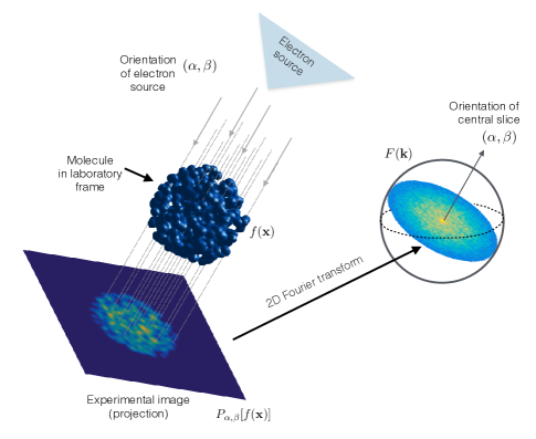
Fig. 1: Illustration of the projection-slice theorem: the 2D Fourier transform of the projection of a compactly supported function $f({\mathbf{x}})$ equals a central slice of the Fourier transform $F({\mathbf{k}})$ through the origin, with normal vector $(1,\alpha,\beta)$.

The proof of this theorem is straightforward (see, for example, (Natterer, )). There is a third angular degree of freedom which must be taken into account in cryo-EM, easily understood by inspection of Fig. 1. In particular, any rotation of the image plane about the orientation vector $(\alpha,\beta)$ could be captured during the experiment.

To take this rotation into account, we need to be more precise about the polar coordinate system $(r,\psi)$ in the image plane. We will denote by $\psi$ the angle subtended in the image plane relative to the projection of the negative $z$-axis in the fixed laboratory frame. (In the case of projections with directions passing through the poles $\alpha=0$ and $\pi$, the above definition becomes ambiguous, and one may set $\psi$ to be the standard polar angle in the $xy$ plane.) Then $\gamma$ specifies in-plane rotation of a projection. Thus, the full specification of an arbitrary projection takes the form

$$P_{\alpha,\beta,\gamma}[f](r,\psi)\;=\;P_{\alpha,\beta}[f](r,\psi-\gamma)~{}.$$ (3)

Remark 2.

The angles $(\alpha,\beta,\gamma)$ correspond to a particular choice of Euler angles that define an arbitrary rotation of a rigid body in three dimensions. The notation introduced here is most convenient for the purposes of our method (corresponding to an extrinsic rotation of $\alpha$ about the $y$ axis, an extrinsic rotation of $\beta$ about the $z$ axis, and an intrinsic rotation of $\gamma$ about the new $z$ axis).

We will denote the set of experimental images obtained from electron microscopy (the input data) by $\bm{\mathfrak{M}}$, with the total number of images given by $M=|\bm{\mathfrak{M}}|$. Each image ${\cal M}^{(m)}\in\bm{\mathfrak{M}}$ has support in the unit disc. We will often omit the superscript $(j)$ when the context is clear. Representing the image in Cartesian coordinates, we let ${\widehat{{\cal M}}}^{(m)}$ denote its 2D Fourier transform in polar coordinates:

$${\widehat{{\cal M}}}^{(m)}(k,\psi)=\int_{-1}^{1}\int_{-1}^{1}{\cal M}^{(m)}(x,y)e^{ik(\cos\psi\,x+\,\sin\psi\,y)}\,dx\,dy.$$ (4)

2.2 Discretization

We discretize the full three-dimensional Fourier transform domain (${\mathbf{k}}$-space) in spherical coordinates as follows. We choose $N_{r}$ equispaced quadrature nodes in the radial direction, between zero and a maximum frequency $K$. The latter sets the achievable resolution. On each sphere of radius $k$, we form a 2D product grid from $N_{\phi}$ equispaced points in the $\phi$ direction, and the following $N_{\theta}$ equispaced points in the $\theta$ direction:

$$\theta_{j}=\frac{(2j-1)\pi}{2N_{\theta}}~{},\qquad 1\leq j\leq N_{\theta}~{}.$$

Writing the volume element $k^{2}\sin\theta\,d\theta\,d\phi\,dk$ as $k^{2}d\mu\,d\phi\,dk$ where $\mu=\cos\theta$ is the scaled $z$-coordinate, we note that the scaled $z$-coordinates of the nodes $\mu_{j}=\cos\theta_{j}$ are thus located at the classical (first kind) Chebyshev nodes on $[-1,1]$. The advantage of this particular choice for $\theta$ (or $\mu$) nodes is that they will be convenient later for local interpolation in $\theta$ near the poles.

The complete spherical product grid of $N_{r}N_{\theta}N_{\phi}$ nodes is used for ${\mathbf{k}}$-space quadrature, with the weight associated with each node being $(2\pi/N_{\phi})k^{2}w_{j}$, where $w_{j}$ is the weight corresponding to the node $\mu_{j}$ on $[-1,1]$. (Here the $\mu$ quadrature is sometimes known as Fejér’s first rule kink .) In particular, this quadrature will be used in computing the final density in physical space by means of the inverse Fourier transform (2).

It is important to note that, because the support of $f$ is in the unit ball, we have very precise bounds on the smoothness of $F({\mathbf{k}})$. Namely, $F$, as a function of ${\mathbf{k}}$, is bandlimited to unit “frequency” (note that here, and here only, we use “frequency” in the reverse sense to indicate the rate of oscillation of $F$ with respect to the Fourier variable ${\mathbf{k}}$). Furthermore, for targets ${\mathbf{x}}$ in the unit ball, the same is true of the exponential function in (2). Thus, the integrand is bandlimited to a “frequency” of 2. This means that the above quadrature scheme is superalgebraically convergent with respect to $N_{\phi}$ and $N_{\theta}$, due to well-known results on the periodic trapezoid and Chebyshev-type quadratures kink . Furthermore, for oscillatory periodic band-limited functions, the periodic trapezoid rule reaches full accuracy once “one point per wavelength” is exceeded for the integrand PTRtref (note that this is half the usual Nyquist criterion). These results are expected to carry over to the spherical sections of 3D bandlimited functions that we use, allowing for superalgebraic error terms. Since the most oscillation with respect to $\theta$ and $\phi$ occurs on the largest $k$ sphere, the above sampling considerations imply $N_{\phi}\geq 2K$ and $N_{\theta}\geq K$. In practice, to ensure sufficient accuracy, we choose values slightly (i.e., up to a factor 1.5) larger than these bounds.

Remark 3.

In practice, the sphere can be sampled more uniformly and more efficiently by choosing $N_{\theta}$ to vary with $k$ and by reducing the number of azimuthal points $N_{\phi}$ near the poles. For simplicity of presentation, we keep them fixed here (see section 8 for further discussion).

Quadrature in the $k$ direction is only second order accurate, as we are relying on the trapezoidal rule with an equispaced grid. Spectral convergence could be achieved using Gauss-Legendre quadrature, but we find that accuracy with a regular grid is sufficient using a node spacing $\delta k:=K/N_{r}\approx 2$, so that $N_{r}=O(K)$.

In our model, rather than using the spherical grid points themselves to sample $F({\mathbf{k}})$, we will, for the most part, make use of a spherical harmonic representation. That is, for each fixed radial value $k$, we will represent $F(k,\theta,\phi)$ on the corresponding spherical shell in the form

$$F(k,\theta,\phi)=\sum_{n=0}^{p(k)}\sum_{m=-n}^{n}f_{nm}(k)Y_{n}^{m}(\theta,\phi)\,.$$ (5)

Here,

$$Y_{n}^{m}(\theta,\phi)=S_{n}^{m}P_{n}^{|m|}(\cos\theta)e^{im\phi}\,,$$ (6)

where $P_{n}(x)$ denote the standard Legendre polynomial of degree $n$, the associated Legendre functions $P_{n}^{m}$ are defined by the Rodrigues’ formula

$$P_{n}^{m}(x)=(-1)^{m}(1-x^{2})^{m/2}\frac{d^{m}}{dx^{m}}P_{n}(x),$$

and

$$S_{n}^{m}=\sqrt{\frac{2n+1}{4\pi}}\sqrt{\frac{(n-|m|)!}{(n+|m|)!}}\,.$$ (7)

The functions $Y_{n}^{m}$ are orthonormal with respect to the $L_{2}$ inner product on the unit sphere

$$\langle f,g\rangle=\int_{0}^{2\pi}\int_{0}^{\pi}f(\theta,\phi)g(\theta,\phi)\sin\theta\,d\theta\,d\phi\,.$$ (8)

Remark 4.

Note that the degree of the expansion in (5) is a function of $k$, denoted by $p(k)$. It is straightforward to show that spherical harmonic modes of degree greater than $k$ are exponentially decaying on a sphere of radius $k$ given that the original function $f(x,y,z)$ is supported in the unit ball in physical space. This is the same argument used in discussing grid resolution above for $N_{r}$, $N_{\phi}$ and $N_{\theta}$. In short, an expansion of degree $O(k)$ is sufficient and, throughout this paper, we simply fix the degree $p(k)=k+2$.

Remark 5.

The orthogonality of the $Y_{n}^{m}$ allows us to obtain the coefficients of the spherical harmonic expansion $f_{nm}$ above via projection. Moreover, separation of variables permits all the necessary integrals to be computed in $O(p(k)^{3})$ operations.

3 Template generation

In any projection matching procedure, a recurring task is that of template generation. That is, given a current model defined by $f({\mathbf{x}})$ or $F({\mathbf{k}})$, we must generate a collection of projection images of the model for a variety of orientation vectors. We will denote those orientations by $(\alpha_{i},\beta_{j})$, leaving $(\theta,\phi)$ to refer to the angular coordinates in Fourier space for a fixed frame of reference. From the projection-slice theorem (Theorem 1), we have

$$\widehat{P_{\alpha_{i},\beta_{j}}[f]}=S_{\alpha_{i},\beta_{j}}[F]~{}.$$

In fact, our projection matching procedure will work entirely in 2D Fourier space, ie using $\widehat{P_{\alpha_{i},\beta_{j}}[f]}(k,\psi)$, where $(k,\psi)$ are polar coordinates in the projection plane, so our task is simply to compute the central slice $S_{\alpha_{i},\beta_{j}}[F]$ on a polar grid for each $i$ and $j$ (see Fig. 2). The real-space projections $P_{\alpha_{i},\beta_{j}}[f]$ will not be needed.

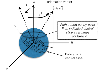
Fig. 2: To generate templates for projection matching, we need to sample the central slice $S_{\alpha,\beta}[F]$ on a polar grid for every orientation vector $(\alpha,\beta)$. The process is accelerated by observing that the $z$-coordinate for any such target point depends only on $\alpha$ and not on $\beta$. This permits the effective use of separation of variables (eq. (3)).

In order to generate all templates efficiently, let a discrete set of desired orientation vectors be denoted by $\{(\alpha_{i},\beta_{j})|\,i=1,\dots,N_{\theta},j=1,\dots,N_{\phi}\}$. We have found that, to achieve acceptable errors at realistic noise levels, these grid sizes $N_{\theta}$ and $N_{\phi}$ can be chosen to be the same as for the quadrature points via the Nyquist criterion in the previous section. Each $\alpha$ corresponds to an initial rotation about the $y$-axis in the laboratory frame, while each $\beta$ corresponds to a subsequent rotation about the $z$-axis in the laboratory frame. (The fact that projection matching can be simplified by creating a sufficiently fine grid on the sphere was already discussed and used in (Penczek1992, ; Penczek1994, ).)

To generate the points at a given radius $k$ within each slice, we must parametrize points in a polar coordinate system on the equatorial plane in the laboratory frame that have been rotated through the preceding actions. Using Cartesian coordinates for the moment, it is easy to see that

$$\left(\begin{array}[]{c}k\cos\psi\\ k\sin\psi\\ 0\end{array}\right)\ \xrightarrow{\alpha\ {\rm rotation}}\ \left(\begin{array}[]{c}k\cos\alpha\cos\psi\\ k\sin\psi\\ -k\sin\alpha\cos\psi\end{array}\right)\ \xrightarrow{\beta\ {\rm rotation}}\ \left(\begin{array}[]{c}k[\cos\beta\cos\alpha\cos\psi-\sin\beta\sin\psi]\\ k[\sin\beta\cos\alpha\cos\psi+\cos\beta\sin\psi]\\ k[-\sin\alpha\cos\psi]\end{array}\right).$$

Note that the $z$ coordinate (and therefore the spherical coordinate $\theta$) in the laboratory frame is independent of $\beta$, while the $x,y$ coordinates in the laboratory frame depend on $\alpha$, $\beta$ and $\psi$.

For each sampled normal orientation vector $(\alpha_{i},\beta_{j})$ for the slice, let $\{\psi_{l}|l=1,\ldots,N_{\phi}\}$ denote equispaced points on $[0,2\pi]$. From above, the sample points with radius $k$, which are located at $(k\cos\psi_{l},k\sin\psi_{l},0)$ before rotation, move to

$$\left(\begin{array}[]{c}x_{ijl}\\ y_{ijl}\\ z_{il}\end{array}\right)=\left(\begin{array}[]{c}k[\cos\beta_{j}\cos\alpha_{i}\cos\psi_{l}-\sin\beta_{j}\sin\psi_{l}]\\ k[\sin\beta_{j}\cos\alpha_{i}\cos\psi_{l}+\cos\beta_{j}\sin\psi_{l}]\\ k[-\sin\alpha_{i}\cos\psi_{l}]\end{array}\right).$$

Fixing the radius $k$ for now, we denote the spherical coordinates of these points $(x_{ijl},y_{ijl},z_{il})$ by $(k,\theta_{il},\phi_{ijl})$. To generate the template data, we now need to evaluate the spherical harmonic expansion at these points, namely

$$F(k,\theta_{il},\phi_{ijl}) =\sum_{n=0}^{p(k)}\sum_{m=-n}^{n}f_{nm}(k)Y_{n}^{m}(\theta_{il},\phi_{ijl})$$

$$=\sum_{m=-n}^{n}A_{iml}e^{im\phi_{ijl}}$$ (9)

for $i=1,\dots,N_{\theta}$ and $j=1,\dots,N_{\phi}$, where

$$A_{iml}=\sum_{n=|m|}^{p(k)}f_{nm}(k)S_{n}^{m}P_{n}^{m}(\cos\theta_{il}).$$

Note that only the degrees at least as large as the magnitude of the order $|m|$ contribute. For each radius $k$, the cost of computing the set $\{A_{iml}\}$ is $O(N_{\theta}N_{\phi}p(k)^{2})$ and the cost of the subsequent evaluation of all values $F(k,\theta_{il},\phi_{ijl})$ is $O(N_{\theta}N_{\phi}^{2}p(k))$. Since $p(k)=O(K)$, both terms have the asymptotic complexity $O(K^{4})$. This generates $O(K^{3})$ template data points on a single spherical shell. Then, summing over all $k$ shells, the cost to generate the full spherical grid templates up to a resolution of $K$ requires $O(K^{5})$ work, and generates $O(K^{4})$ data.

Letting $k_{q}\in\{k_{1},\dots,k_{N_{r}}\}$ denote the discretization in $k$, the above procedure evaluates the $O(K^{2})$ samples comprising the polar grid $(k_{q},\psi_{l})$, for each of the $O(K^{2})$ central slices. However, it is more convenient to store these templates in terms of their angular Fourier series for each slice, ie,

$$S_{\alpha_{i},\beta_{j}}[F](k_{q},\psi)=\sum_{n=-N_{q}}^{N_{q}}S^{ij}_{n}(k_{q})e^{in\psi},$$ (10)

with $2N_{q}+1$ Fourier modes used on the $q$th ring. By band-limit considerations of the spherical harmonics, one need only choose $N_{q}=p(k_{q})$, the maximum degree for each $k$ shell.

The coefficients $S^{ij}_{n}(k_{q})$ are evaluated by applying the fast Fourier transform (FFT) to the template data along the $\psi$ grid direction, requiring $O(K^{4}\log K)$ work.

4 Projection matching

Given an experimental image ${\cal M}\in\bm{\mathfrak{M}}$ (or more precisely its 2D Fourier transform ${\widehat{{\cal M}}}(k,\psi)$ discretized on a polar grid), we seek to rank the templates defined by $(\alpha_{i},\beta_{j})$ and the rotational degree of freedom $\gamma$ in terms of how well they match the image. For this we need a generative model for images. We will then present an algorithm for matching $\gamma$.

4.1 Image model with CTF correction

For reasons having to do with the physics of data acquisition, each particle image ${\cal M}^{(m)}$ is not simply a projection of the electron-scattering density, but may be modeled as the projection of the electron-scattering density convolved with a contrast transfer function (CTF) (Mindell2003, ), plus noise. The CTF includes diffraction effects due to the particle’s depth in the ice sheet, linear elastic and inelastic scattering, and detection effects. In the simplest case, the CTF is radially symmetric and its Fourier transform is real-valued and of the form $C^{(m)}(k)$, depending only on $k$. For the purposes of the present paper, we will assume that $C^{(m)}(k)$ is known for each experimental image. By the convolution theorem, the CTF acts multiplicatively on the Fourier transform image. Thus, the expectation for the $m$th Fourier image given by beam direction $(\alpha,\beta)$ and in-plane rotation $\gamma$, deriving from a ${\mathbf{k}}$-space scattering density $F$, is

$${\widehat{{\cal M}}}^{(m)}(k,\psi-\gamma)\;\approx\;C^{(m)}(k)S_{\alpha,\beta}[F](k,\psi)~{}.$$

To this is added measurement noise, which is assumed to be Gaussian and i.i.d. on each pixel in the image.

4.2 Fitting the best orientation for each image

It would follow from the above noise model that the correct quantity to minimize when searching for the best match would be the $L_{2}$ norm of the difference between the template and the image, which is equivalent to the $L_{2}$ norm of their difference in the Fourier image plane. This may be interpreted as minimizing the negative log likelihood, i.e. finding the maximum likelihood. Let ${\widehat{{\cal M}}}={\widehat{{\cal M}}}^{(m)}$ be the current experimental image in question, and $C=C^{(m)}$ be its corresponding known CTF. We will denote by ${\widehat{{\cal M}}}_{\gamma}$ the rotated Fourier image

$${\widehat{{\cal M}}}_{\gamma}(k,\psi):={\widehat{{\cal M}}}(k,\psi-\gamma)~{}.$$

For the template index pair $(i,j)$, a quantity to be minimized over the rotation $\gamma$ would thus be

$$\|{\widehat{{\cal M}}}_{\gamma}-CS_{\alpha_{i},\beta_{j}}[F]\|_{2},$$ (11)

where, for a function $g(k,\gamma)$ in polar coordinates, the $L_{2}$ norm (up to a band-limit of $K$) is defined by

$$\|g\|^{2}:=\int_{0}^{K}\int_{0}^{2\pi}|g(k,\psi)|^{2}d\psi kdk.$$ (12)

However, there is typically uncertainty about the overall normalization (a multiplicative prefactor) associated with experimental images (as discussed for instance by Scheres et al. Scheres2009 ). It is straightforward to check that minimizing (11) over $i,j,\gamma$ including an unknown normalization factor for the image is equivalent to maximizing over $i,j,\gamma$ the normalized inner product

$$\frac{\langle CS_{\alpha_{i},\beta_{j}}[F],{\widehat{{\cal M}}}_{\gamma}\rangle}{\|CS_{\alpha_{i},\beta_{j}}[F]\|\,\|{\widehat{{\cal M}}}_{\gamma}\|}~{}.$$ (13)

Here the inner product corresponds to the norm (12), and (13) may be interpreted as the cosine of the “angle” between the image and the template in the abstract vector space with norm (12). Maximizing (13) over $i,j$ and $\gamma$ we refer to as projection matching.

For each $k_{q}\in\{k_{1},\dots,k_{N_{r}}\}$, we precompute a Fourier series representation of the image, with $2N_{q}+1$ Fourier modes on the $q$th ring:

$${\widehat{{\cal M}}}(k_{q},\psi)=\sum_{n=-N_{q}}^{N_{q}}{\widehat{{\cal M}}}_{n}(k_{q})e^{in\psi}.$$

This requires $O(K^{2}\log K)$ work, done once for each experimental image.

To rank the template matches we loop over all projection directions indexed by $i,j$. For each of these directions $(\alpha_{i},\beta_{j})$, since the denominator of (13) is fixed, we need to maximize the inner product as a function of $\gamma$,

$$\langle CS_{\alpha_{i},\beta_{j}}[F],{\widehat{{\cal M}}}_{\gamma}\rangle:=\int_{0}^{K}\int_{0}^{2\pi}{\widehat{{\cal M}}}(k,\psi-\gamma)\overline{C(k)\,S_{\alpha_{i},\beta_{j}}[F](k,\psi)}d\psi kdk.$$

Elementary Fourier analysis shows that

$$\langle CS_{\alpha_{i},\beta_{j}}[F],{\widehat{{\cal M}}}_{\gamma}\rangle=\sum_{n}c_{n}(K)e^{-in\gamma}$$

where

$$c_{n}(\kappa):=\int_{0}^{\kappa}{\widehat{{\cal M}}}_{n}(k)\overline{C(k)S^{ij}_{n}(k)}kdk.$$ (14)

This integral is approximated using the existing $k$ grid up to the maximum frequency $\kappa=O(K)$, requiring $O(K^{2})$ effort to compute the $2N_{q}+1$ coefficients. Since there are $O(K^{2})$ pairs $i,j$, this totals $O(K^{4})$ work per experimental image. Finally, for each pair $i,j$, we will compute the best value for $\gamma$ by tabulating $\sum_{n}c_{n}(K)e^{-in\gamma}$ on a uniform grid of $N_{\phi}$ values, using the FFT, and taking the index with the maximum modulus. This requires $O(K^{3}\log K)$ work per image. Thus, the complexity for angle fitting all images is $O(MK^{4})$.

Definition 3.

The best values of $(\alpha,\beta,\gamma)$ for image ${\cal M}^{(m)}$ will be denoted by ${\cal A}_{m}=(\alpha_{m},\beta_{m},\gamma_{m})$.

In practice we implement two useful adjustments to the above procedure:

1) We search first over a coarse grid of template directions (with angle resolution 5 times coarser than the grid defined by $N_{\theta}$ and $N_{\phi}$), and then only search over the set of grid points that are within one coarse grid point of the global maxima found on the coarse grid. This improves efficiency by a constant factor, and in our tests does not degrade accuracy noticeably.

2) We define a “randomization parameter” $f_{rand}$. If $f_{rand}=0$, we return the single best-fitting orientation: $(\alpha_{m},\beta_{m},\gamma_{m})$ defined above. However, if $f_{rand}>0$, we instead choose ${\cal A}_{m}$ randomly from the set of all discrete orientations $(\alpha,\beta,\gamma)$ that produce a normalized inner product (13) greater than $1-f_{rand}$. Typically we choose $f_{rand}$ small, e.g. 0.02. This uniformizes the distribution of orientations over the set which fit the image almost equally well. However, it is sometimes beneficial to increase $f_{rand}$ for improved convergence rate in the least-squares procedure of the following section; see section 7.3.

It should be noted that the idea of using Fourier methods to find the optimal third Euler angle $\gamma$ can be found in (Cong2003, ), and the complexity of various alignment schemes using polar grids in physical space is discussed in (Joyeux2002, ).

Remark 6.

In the simplest version of the frequency marching scheme we present, the $c_{n}$ coefficients in (14) are evaluated using all frequencies from zero to $\kappa$, since $F$, and hence the templates, get updated over this frequency range each iteration. We believe that updating the model $F$ only in the current $k$ shell could result in a faster algorithm without sacrificing accuracy. In that case, the $c_{n}$ values are already known for a smaller $\kappa$, and they can be incremented according to the formula

$$c_{n}(\kappa_{2})=c_{n}(\kappa_{1})+\int_{\kappa_{1}}^{\kappa_{2}}{\widehat{{\cal M}}}_{n}(k)\overline{C(k)S^{ij}_{n}(k)}kdk\,.$$

5 Reconstruction from particle images with known angular assignments

Suppose now that we have the collection of Fourier transforms of all $M$ particle images, which we denote by

$${\widehat{\bm{\mathfrak{M}}}}\;:=\;\{{\widehat{{\cal M}}}^{(1)}(k,\psi),{\widehat{{\cal M}}}^{(2)}(k,\psi),\dots,{\widehat{{\cal M}}}^{(M)}(k,\psi)\},$$

together with the corresponding angular assignments ${\cal A}=\{{\cal A}_{1},{\cal A}_{2},\dots,{\cal A}_{M}\}$, where ${\cal A}_{m}=(\alpha_{m},\beta_{m},\gamma_{m})$.

Remark 7.

In our present implementation, the values of $(\alpha_{m},\beta_{m},\gamma_{m})$ are selected from the set of computed template angles, as discussed in the previous section. A more sophisticated projection matching procedure could generate “off-grid” values for $\alpha,\beta$, and $\gamma$. The reconstruction procedure below works in either case.

We seek to reconstruct a (new) model $F(k,\theta,\phi)$ that is consistent with all of the data in a least squares sense. For each fixed spherical shell of radius $k$, we use the representation (5), and data ${\widehat{{\cal M}}}^{(m)}_{\gamma_{m}}(k,\psi)$ which, if the angle assignments are correct, is expected to approximate the CTF-corrected central slice $C^{(m)}(k)S_{\alpha_{m},\beta_{m}}[F](k,\psi)$ for the new model. The matching between the new model and the image data on the $k$ shell is done at a set of $N_{\phi}$ discrete angles $\phi_{l}$ on each great circle. The Cartesian coordinates of those points are

$$\left(\begin{array}[]{c}k[\cos\beta_{m}\cos\alpha_{m}\cos\psi_{l}-\sin\beta_{m}\sin\psi_{l}]\\ k[\sin\beta_{m}\cos\alpha_{m}\cos\psi_{l}+\cos\beta_{m}\sin\psi_{l}]\\ k[-\sin\alpha_{m}\cos\psi_{l}]\end{array}\right),$$ (15)

from which their spherical coordinates $(\theta_{ml},\phi_{ml})$ are easily computed. Thus, for the Fourier sphere of radius $k$, each image contributes $N_{\phi}$ points, for a total of $N_{tot}=MN_{\phi}$ points on this sphere.

At this stage, we simply collect all image data with given $k$ into a right-hand side vector ${\mathbf{d}}$, defined by its $N_{tot}$ entries

$$d_{(m-1)N_{\phi}+l}={\widehat{{\cal M}}}^{(m)}_{\gamma_{m}}(k,\psi_{l})~{},\qquad\mbox{ for }m=1,\dots,M,\quad l=1,\ldots,N_{\phi}~{}.$$

From now we shall use a single index $i=1,\ldots,N_{tot}$ to reference these entries, and use $(\theta_{i},\phi_{i})$ for the spherical coordinates for the corresponding point on the great circle. (In our present implementation we ignore the use of image normalization factors that could be extracted from the orientation fitting algorithm presented in section 4.2. This is justified since our synthetic noisy images will be generated without varying normalization factors.)

Let ${\mathbf{f}}$ denote the vector of “unrolled” spherical harmonic coefficients in the representation for $F$ on the current $k$ sphere,

$${\mathbf{f}}=\{f_{0,0}(k),f_{1,-1}(k),f_{1,0}(k),f_{1,1}(k),f_{2,-2}(k),\dots,f_{p(k),p(k)}(k)\}~{},$$

so that ${\mathbf{f}}$ is a complex vector of length $(p(k)+1)^{2}$. Then we define the complex-valued matrix S, of dimension $N_{tot}\times(p(k)+1)^{2}$, by

$$(S\,{\mathbf{f}})_{i}=\sum_{n=0}^{p(k)}\sum_{m=-n}^{n}f_{nm}(k)Y_{n}^{m}(\theta_{i},\phi_{i})\,.$$ (16)

Thus, $S$ evaluates the spherical harmonic expansion with coefficients ${\mathbf{f}}$ at all sphere points. We also let $C_{i}(k)$ be the corresponding CTF for each image at frequency $k$ (note that $C_{i}(k)$ is the same for all $i$ belonging to the same image), and let ${\cal C}$ be the diagonal matrix with diagonal entries $C_{i}(k)$. We find the desired solution by solving the problem

$${\cal C}S{\mathbf{f}}={\mathbf{d}}$$

in a least squares sense. Note that the use of the $l^{2}$ norm corresponds to the same assumption of i.i.d. Gaussian noise on the images as in the previous section.

For this, we use conjugate gradient (CG) iteration on the normal equations

$$S^{H}{\cal C}^{H}{\cal C}S\,{\mathbf{f}}=S^{H}{\cal C}^{H}{\mathbf{d}},$$

where $S^{H}$ is the Hermitian transpose of $S$. Applying the diagonal matrices ${\cal C}$ and ${\cal C}^{H}$ is trivial. Direct computation of the matrix-vector product with $S$ or $S^{H}$ would require $O(M\,N_{\phi}\,(p(k)+1)^{2})=O(MK^{3})$ work. The application of $S$ is easily accelerated, however, by first evaluating the spherical harmonic expansion induced by ${\mathbf{f}}$ on a regular grid with $N_{\phi}$ equispaced points in the $\phi$ direction, and $N_{\theta}$ points in the $\theta$ direction whose cosines are classical Chebyshev nodes (see section 2.2). Using separation of variables, this requires $O(K^{3})$ work, since $N_{\phi}=N_{\theta}=O(K)$. The value of $S\,{\mathbf{f}}$ at an arbitrary point can then be computed by local $q$th-order Lagrange interpolation in $\phi$ and $\theta$ from this regular grid, at a cost of $q^{2}$ operations per target. It is sufficient to use $q$ in the range 5 to 10. We denote by $S_{reg}$ the mapping from spherical harmonic coefficients to values on the $N_{\phi}\times N_{\theta}$ grid, and by $T$ the (sparse) interpolation matrix from the $N_{\phi}\times N_{\theta}$ grid points to the $N_{tot}$ arbitrary locations. In other words, up to interpolation error,

$$S{\mathbf{f}}\approx TS_{reg}{\mathbf{f}},$$

and applying $S$ in this manner requires only $O(Mq^{2}K+K^{3})$ work. Clearly,

$$S^{H}{\cal C}^{H}{\cal C}S\approx S^{H}_{reg}T^{H}{\cal C}^{H}{\cal C}TS_{reg},$$

where $S^{H}_{reg}$ can be applied by projection from a regular grid to a spherical harmonic expansion, which is also $O(K^{3})$. Thus each CG iteration requires only $O(Mq^{2}K+K^{3})$ work. So long as the $N_{tot}$ points have reasonable coverage of the sphere (specifically that there are no large “pockets” on the sphere which are empty of points), the system is well conditioned and requires only a modest number of iterations, around 20–50, to achieve several digits of accuracy. It is worth noting (as in other Fourier-based schemes, such as FREALIGN (Grigorieff2007, ; Grigorieff2016, ; Lyumkis2013, )) that this least squares procedure is the step in the reconstruction that is responsible for denoising. The more experimental images that are available (with poor signal-to-noise ratios but correctly assigned angles), the more accurately we are able to estimate ${\mathbf{f}}$, hence $F({\mathbf{k}})$ and the electron-scattering density $f({\mathbf{x}})$.

The above describes the computation of $F$ on a single $k$ shell. One advantage of our representation is that to build the complete new model $F$, the least squares solve for each $k$ shell in the grid $\{k_{1},\ldots,k_{N_{r}}\}$ may be performed independently. This gives an overall complexity for the reconstruction of $O(Mq^{2}K^{2}+K^{4})$.

Definition 4.

Let ${\mathbf{F}}$ indicate the entire set of model coefficients $\{{\mathbf{f}}(k_{1}),\ldots,{\mathbf{f}}(k_{N_{r}})\}$. We will refer to its least squares approximation (on all $k$ shells) by ${\mathbf{F}}^{*}$. We summarize this by

$${\mathbf{F}}^{*}=L({\widehat{\bm{\mathfrak{M}}}},{\cal A}):=\arg\min_{{\mathbf{F}}}\sum_{m=1}^{M}\|{\cal C}^{(m)}S_{{\cal A}_{m}}({\mathbf{F}})-{\widehat{{\cal M}}}^{(m)}\|_{2}^{2}\,,$$ (17)

where ${\cal C}^{(m)}$ is the CTF for the $m$th image and, by analogy with (3), $S_{{\cal A}_{m}}({\mathbf{F}})$ denotes the slice

$$S_{{\cal A}_{m}}[F]=\widehat{P_{\alpha_{m},\beta_{m},\gamma_{m}}[f]}~{}.$$

Here, $F$ is determined from the coefficients ${\mathbf{F}}$ via the spherical harmonic representation (5).

6 The full inverse problem

As discussed in the previous section, if the angular assignments ${\cal A}=\{{\cal A}_{1},..,{\cal A}_{M}\}$ of the experimental images were given, ${\mathbf{F}}$ could be recovered by solving the least squares problem (17). Since the angles ${\cal A}$ are unknown, however, it is standard to write the cryo-EM reconstruction problem in terms of the nonlinear and nonconvex optimization task in the joint set of unknowns:

$$\{{\mathbf{F}}^{*},{\cal A}^{*}\}=\arg\min_{\{{\mathbf{F}},{\cal A}\}}\sum_{m=1}^{M}\|{\cal C}^{(m)}S_{{\cal A}_{m}}({\mathbf{F}})-{\widehat{{\cal M}}}^{(m)}\|_{2}^{2}\,.$$ (18)

As noted above, for simplicity of presentation of the scheme, we omit image normalization prefactors discussed in section 4.2.

One well-known approach to solving (18) is to start with an initial guess ${\mathbf{F}}^{(0)}$ for the representation ${\mathbf{F}}$, then to iterate as follows:

Classical iterative refinement Set $i=1$. While (convergence criterion has not been met), 1. Compute ${\cal A}^{(i)}$ from ${\mathbf{F}}^{(i-1)}$ by projection matching (section 4). 2. Set ${\mathbf{F}}^{(i)}=L({\widehat{\bm{\mathfrak{M}}}},{\cal A}^{(i)})$ by least squares solution (section 5). 3. $i\leftarrow i+1$. Compute $F$ from the final ${\mathbf{F}}$ via (5) then take the inverse Fourier transform (2) to recover $f$.

This iteration can be viewed as coordinate descent, alternating between fitting the best angle assignment and fitting the best model density. It will converge, but to a local minimum—not necessarily the correct solution (Cheng2015, ). Various attempts to overcome this convergence failure have been proposed, including annealing strategies and stochastic hill climbing (see, for example, (Elmlund2012, ; Cheng2015, )), but robustness has remained an issue.

6.1 Frequency marching (recursive linearization)

As in the iteration above, we alternate between projection matching to obtain estimates for the angles ${\cal A}$ and solving least squares problems to determine the best set of density coefficients ${\mathbf{F}}$. However, by continuously increasing the resolution—measured in terms of the maximal spatial frequency used in the representation for ${\mathbf{F}}$—we bypass the difficulties associated with multiple minima in existing attempts at iterative refinement. In the language of optimization, this can be viewed as a homotopy method using the maximum spatial frequency (resolution) as the homotopy parameter. The basic intuition underlying our scheme is motivated by the success of recursive linearization in inverse acoustic scattering (BaoLi2015, ; Borges2016, ; Chenrep1088, ; Chen, ).

More precisely, let ${\widehat{\bm{\mathfrak{M}}}}([0,k])$ denote the set of Fourier transforms of all experimental images restricted to the disk of radius $k$, and let ${\mathbf{F}}([0,k])$ denote the density coefficients only up to frequency $k$, i.e. using the shells for which $k_{q}\leq k$. The full objective function minimization restricted to maximum frequency $k$ is

$$\{{\mathbf{F}}^{*}([0,k]),{\cal A}^{*}\}=\arg\min_{\{{\mathbf{F}}([0,k]),{\cal A}\}}\sum_{m=1}^{M}\|{\cal C}^{(m)}S_{{\cal A}_{m}}({\mathbf{F}}([0,k]))-{\widehat{{\cal M}}}^{(m)}([0,k])\|_{2}^{2}~{},$$ (19)

which is still a nonlinear and nonconvex optimization problem. However, if ${\mathbf{F}}([0,k])$ is known and we only seek to find ${\mathbf{F}}([0,k+\delta k])$ for sufficiently small $\delta k$, then the solution can be reached by a suitable linearization. Moreover, at low frequency, say for $k\leq k_{1}=2$, the landscape is extremely smooth so that the global minimum is easily located. Thus, we propose simply assigning random angles ${\cal A}_{m}=(\alpha_{m},\beta_{m},\gamma_{m})$ to the images at $k_{min}=k_{1}=2$ and iterating as follows:

Solution by frequency marching On input, we define a sequence of frequency steps from $k_{1}$ to $k_{N_{r}}=K$ with a step of $\delta k=k_{i+1}-k_{i}$. $\bullet$ Set ${\cal A}^{(0)}$ to uniform random values over the allowed ranges. $\bullet$ Set ${\mathbf{F}}([0,k_{1}])=L({\widehat{\bm{\mathfrak{M}}}}([0,k_{1}]),{\cal A}^{(0)})$ by least squares (section 5). For $i=1,2,\ldots,N_{r}-1,$ 1. Compute ${\cal A}^{(i)}$ from ${\mathbf{F}}([0,k_{i}])$ by projection matching (section 4). 2. Set ${\mathbf{F}}([0,k_{i+1}])=L({\widehat{\bm{\mathfrak{M}}}}([0,k_{i+1}]),{\cal A}^{(i)})$ by least squares (section 5). Compute $F$ from ${\mathbf{F}}([0,K])$ via (5) then take the inverse Fourier transform (2) to recover $f$.

Note that the procedures of sections 4 and 5 restrict naturally to any frequency range $[0,k]$. The key feature of refinement by recursive marching is that it is a deterministic procedure involving only linear solves and angular assignments of images. The overall complexity, combining those from sections 4 and 5, and summing over $k$, is $O(MK^{5}+K^{6}+q^{2}MK^{3})$, where the first two terms come from angle matching and the last from least squares solution. Since in current cryo-EM applications, $K\sim 10^{2}$, while $M\sim 10^{5}$ to $10^{6}$, and $q^{2}<K$, the dominant cost is $O(MK^{5})$, assuming we use the global angle matching procedure described above. However, we find that in our examples, due to the number of CG iterations, the time for least squares fitting is actually quite similar to that for angle matching, i.e. they are close to balanced.

While we are not able to provide a proof in the general case, we believe that under fairly broad conditions this iteration will converge with high probability for sufficiently small $\delta k$ (the radial frequency grid spacing). Informally speaking, we believe that a solution near the global minimum is often reached at low $k$ in the first few iterations and that a path to the global minimum at $K$ is then reached as $k$ increases continuously.

In the experiments below we show that, even with very noisy data, a harsh random start at $k_{min}=2$ is sufficient. We will return to this question in the concluding section.

In practice, we have implemented a further acceleration to the above scheme: if the mean absolute change in angles between ${\cal A}^{(i+1)}$ and ${\cal A}^{(i)}$ is less than $10^{-3}$, the next increment of the index $i$ is set to five rather than its usual value of one. This greatly reduces the number of steps in the marching procedure once the majority of angles have locked in with sufficient accuracy.

7 Numerical experiments with synthetic data

Rubisco	Lipoxygenase-1	Neurotoxin

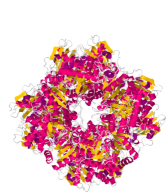
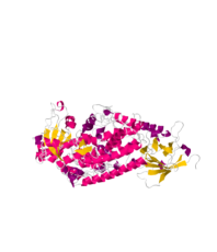
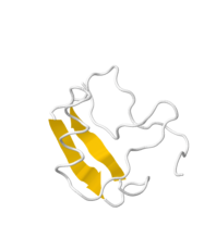
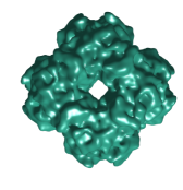
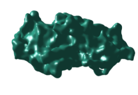
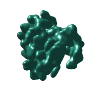
Fig. 3: Top row: The three protein structures (derived from X-ray crystallography). Bottom row: the corresponding atomic densities $f({\mathbf{x}})$ used as a ground truth for the numerical experiments, shown via an isosurface at approximately half the maximum density. Note that the visual length scale for the three molecules is different.

We implemented the above frequency marching algorithm and performed experiments using simulated images to reconstruct electron scattering densities for three proteins.

7.1 Choice of ground-truth densities and error metric

The three proteins we used for numerical experiments were (see Fig. 3): spinach rubisco enzyme (molecular weight 541kDa, 133 Å longest dimension), lipoxygenase-1 (weight 95kDa, 107 Å longest dimension), and scorpion protein neurotoxin (weight 7.2kDa, 33 Å longest dimension). Atomic locations in Å are taken from the protein data bank (PDB) entries pdb , with codes 1RCX, 1YGE, 1AHO, respectively, but were shifted to have their centroid at the origin. Only in the last of the three are hydrogen atom locations included in the PDB. Thus, the number of atoms used were 37456, 6666, and 925, respectively. Note that the last of these, the neurotoxin, is much smaller than the $\approx 100$ kDa lower weight limit that can be imaged through cryo-EM with current detector resolution and motion-correction technology; our point in including it is to show that, given appropriate experimental image resolution, reconstruction of small molecules does not pose an algorithmic problem.

For each protein, a ground-truth electron scattering density $f({\mathbf{x}})$ was produced using the following simple model. Firstly, a non-dimensionalization length $D$ was chosen giving the number of physical Å per unit numerical length, such that the support of $f$ in such numerical units lies within the unit ball. For rubisco, $D=70$ Å, for lipoxygenase-1, $D=60$ Å, and for the neurotoxin, $D=25$ Å. Thus, all physical distances in what follows are divided by $D$ in the numerical implementation. We summed 3D spherically-symmetric Gaussian functions, one at each atomic location, giving each Gaussian a standard deviation $\sqrt{(0.5r)^{2}+b^{2}}$, where $r$ is the atomic radius for the type of atom (which vary from 0.42 Å to 0.88 Å). The factor $0.5$ results in around 74% of the mass of the unblurred Gaussian falling within radius $r$, and $b$ is a convolution (blurring) radius used to make $f$ smooth enough to be accurately reconstructed using the image pixel resolution. The radii $b$ used were 2.5Å for rubisco, 2.0Å for lipoxygenase-1, and 1.0Å for scorpion toxin, chosen to be around twice the simulated pixel spacing (see next section). Thus, when we assess reconstruction errors, we are doing so against an appropriately smoothed ground-truth $f$. For simplicity, each such Gaussian was given a unit peak amplitude.

Our error metric for a reconstructed density $\tilde{f}$ is the relative $L_{2}$-norm,

$$\epsilon:=\frac{\|\tilde{f}-f\|_{L_{2}([-1,1]^{3})}}{\|f\|_{L_{2}([-1,1]^{3})}}~{},$$ (20)

which is estimated using quadrature on a sufficiently fine uniform 3D Cartesian grid (we used $100$ points in each dimension).

Remark 8.

Since $\tilde{f}$ generally acquires an arbitrary rotation $(\alpha,\beta,\gamma)$ relative to the ground-truth $f$, we must first rotate it to best fit the original $f$. This is done by applying the procedure of section 4 to a small number (typically 10) of random projections. $\tilde{f}$ is then rotated using the 3D non-uniform FFT nufft to evaluate its Fourier transform $\tilde{F}$ at a rotated set of spherical discretization points as in section 2.2. A second non-uniform FFT is then applied to transform back to real space. Finally the error (20) is evaluated.

Some researchers use a normalized cross-correlation metric to report errors (eg. Joubert2015 ). We note that, when errors are small, this metric is close to $1-\epsilon^{2}/2$ with $\epsilon$ given by (20).

7.2 Generation of synthetic experimental images

For each of the three proteins, $M$ (of order 50,000) synthetic experimental images were produced as follows. For each image $m$ we first defined a realistic radially-symmetric CTF function $C^{(m)}(k)$ using the standard formulae Mindell2003 ; wade

$$C(k)=B(\theta)[w_{1}\sin\chi(\theta)-w_{2}\cos\chi(\theta)],\quad\mbox{ where }\;\chi(\theta):=\frac{1}{2}kz\theta^{2}+kC_{s}\theta^{4}/8,\quad B(\theta):=e^{-\theta^{2}/\theta_{0}^{2}}~{}.$$ (21)

Here $\chi$ is called the phase function, $\theta_{0}=0.002$ sets the microscope acceptance angle, $w_{2}=0.07$ controls the relative inelastic scattering, with $w_{1}^{2}+w_{2}^{2}=1$, and the spherical aberration is $C_{s}=2\times 10^{7}$ Å. The defocus parameter $z$ was different for each image, chosen uniformly at random in the interval $[1,4]\times 10^{4}$ Å. Finally, in the above, angles $\theta$ are related to wavenumbers $k$ in the numerical experiments via

$$\theta=\frac{\lambda k}{2\pi D}~{},$$ (22)

where $\lambda=0.025$ Å is the free-space electron wavelength (a typical value corresponding to a 200 keV microscope), and for convenience the distance scaling $D$ has been included. In our setting $\theta$ is of order $10^{-5}$ times the numerical wavenumber $k$.

The images were sampled on a uniform 2D grid at a standard resolution of $100\times 100$ pixels covering the numerical box $[-1,1]^{2}$. The pixel spacing thus corresponded to $D/50$, or between 0.5 Å for neurotoxin (this is smaller than currently achievable experimentally) and 1.4 Å for rubisco. The noise-free signal images were produced by inverse Fourier transforming (via the 2D non-uniform FFT) slices taken at random orientations through the ground-truth Fourier density $F({\mathbf{k}})$, after multiplication by the radial CTF $C^{(m)}(k)$ particular to each image. Finally, i.i.d. Gaussian noise was added to each pixel, with variance chosen to achieve a desired signal-to-noise ratio (SNR). SNR has the standard definition in imaging as the ratio of the squared $L_{2}$-norm of the signal to that of the noise (for this we used the domain $[-1,1]^{2}$ since the molecule images occupy a large fraction of this area). We generated images at SNR values of $\infty$ (no noise), 0.5, 0.1 and 0.05. A typical value in applications is 0.1.

7.3 Results

All numerical experiments were run on desktop workstations with 14 cores, Intel Xeon 2.6GHz CPU, and 128 GB RAM. Our implementation is in Fortran, with OpenMP parallelization. We used frequency marching with step size $\delta k=2$, starting with random angular assignment at $k_{1}=2$, and marching to full resolution at $K=70$. This $K$ was sufficient to resolve the decaying tails of $F$ without significant truncation error, given our choice of blurring radius $b$ at approximately two pixels. We used interpolation order $q=7$, and we started with randomization factor $f_{rand}=0.02$. The latter was changed adaptively during marching to balance solution time and accuracy, as follows: if at some point, the least squares CG did not converge after 100 iterations, $f_{rand}$ was doubled and the least squares solve repeated. If instead CG required less than 50 iterations, $f_{rand}$ was halved. The speed of our algorithm allowed us to carry out multiple runs for each protein, using either the same or a fresh set of synthetic images. In the present paper, we carried out 5 runs for each protein.

To assess how close our relative $L_{2}$ error $\epsilon$ was to the best achievable, given the image sampling, Fourier representation, and SNR, we computed for comparison the best possible $\epsilon$ achieved by reconstructing $f$ through a single application of the least squares procedure (section 5) with all image orientations set to their true values. Table 1 shows that the errors resulting from applying our proposed frequency marching algorithm exceed this best possible error by only around $10^{-2}$, for all molecules and noise levels.

Figures 4 c) and d), 5 c) and d) and 6 c) and d) show the results of the reconstruction for the three models using experimental images at SNR 0.5 and 0.05 respectively. Out of the 5 runs, we show the reconstructions with the lowest error. Table 2 shows that it took approximately 2 hours to do the reconstructions using frequency marching on 14 cores for all three models. This table also shows that the time is not significantly affected by the noise levels in the data. In addition, we expect that the quality of the reconstruction will improve as we increase the number of experimental images. This effect is visible in Figure 7, where the median squared error of the runs is surprisingly well fit by the functional form of a constant (accounting for Fourier and image discretization errors) plus a constant times $1/M$, accounting for the usual reduction in statistical variance with a growing data set size $M$.

		No Noise	SNR $0.5$	SNR $0.1$	SNR $0.05$
Rubisco	frequency marching	$0.06\pm 0.001$	$0.06\pm 0.001$	$0.08\pm 0.001$	$0.09\pm 0.004$
	known angles	$0.05$	$0.06$	$0.07$	$0.08$
Lipoxygenase-1	frequency marching	$0.05\pm 0.008$	$0.06\pm 0.002$	$0.09\pm 0.005$	$0.12\pm 0.003$
	known angles	$0.04$	$0.05$	$0.08$	$0.11$
Scorpion toxin	frequency marching	$0.05\pm 0.002$	$0.06\pm 0.003$	$0.06\pm 0.002$	$0.07\pm 0.004$
	known angles	$0.04$	$0.04$	$0.05$	$0.06$

Table 1: Relative $L_{2}$ errors $\epsilon$ (see (20)) of the reconstructions using frequency marching, compared to the best-possible reconstruction using known angles for the experimental images. The frequency marching results are given as averages over 5 runs, with estimated standard deviation.

	No Noise	SNR $0.5$	SNR $0.1$	SNR $0.05$
Rubisco	$1.6\pm 0.5$	$1.4\pm 0.3$	$1.2\pm 0.1$	$1.4\pm 0.1$
Lipoxygenase-1	$1.1\pm 0.4$	$1.5\pm 0.6$	$1.1\pm 0.4$	$1.2\pm 0.3$
Scorpion toxin	$0.5\pm 0.1$	$0.5\pm 0.1$	$0.6\pm 0.1$	$0.7\pm 0.2$

Table 2: Time in hours for the reconstructions on 14 cores, in the context of different levels of noise added to the experimental images. All the times are given as averages with estimated standard deviations, over 5 different runs.

SNR 0.5	SNR 0.05
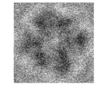
(a)	(b)
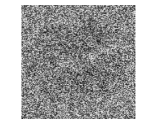
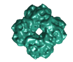
(c)	(d)
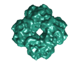
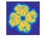
(e)	(f)

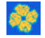
Fig. 4: Results for Rubisco reconstruction. (a,b): Examples of experimental images at SNR 0.5 and 0.05 (black is smallest values, white largest). (c,d): Reconstructions by frequency marching using experimental images at SNR 0.5 and 0.05, shown as isosurfaces. (e,f): Examples of a single slice through the reconstructed $f$ (blue is smallest values, yellow largest).

SNR 0.5	SNR 0.05
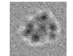
(a)	(b)
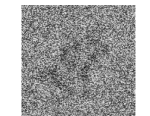
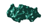
(c)	(d)
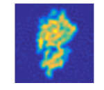
(e)	(f)

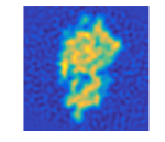
Fig. 5: Results for lipoxygenase-1 reconstruction. (a,b): Examples of experimental images at SNR 0.5 and 0.05. (c,d): Reconstructions by frequency marching using experimental images at SNR 0.5 and 0.05, shown as isosurfaces. (e,f): Examples of a single slice through the reconstructed $f$.

SNR 0.5	SNR 0.05
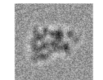
(a)	(b)
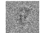
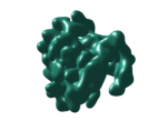
(c)	(d)
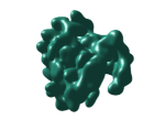
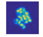
(e)	(f)

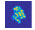
Fig. 6: Results for scorpion toxin reconstruction. (a,b): Examples of synthetic experimental images at SNR 0.5 and 0.05. (c,d): Reconstructions by frequency marching from experimental images at SNR 0.5 and 0.05, shown as isosurfaces. (e,f): Examples of a single slice through the reconstructed $f$.

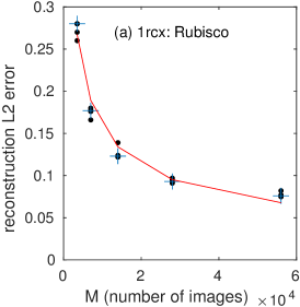
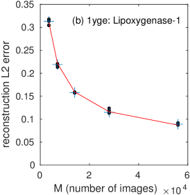
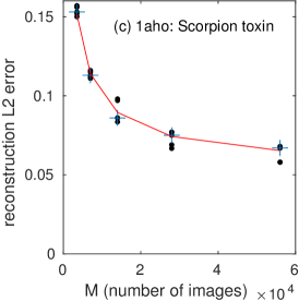
Fig. 7: Relative $L_{2}$-error $\epsilon$ of the reconstructed model (see (20)) vs $M$, the number of simulated experimental images used for the reconstruction (black dots), using five runs for each of the three molecules. The SNR is 0.05. The error decreases as $M$ increases. The median is also shown (plus signs), as is the best fit to the expected form $a_{0}+a_{1}/M$ for the square of the median errors. (Two of the runs failed with our random initialization procedure and are not shown on this figure).

8 Conclusions

We have presented a fast, robust algorithm for determining the three-dimensional structure of proteins using “single particle” cryo-electron microscopy (cryo-EM) data. This problem is typically formulated in the language of global optimization, leading to a non-convex objective function for the unknown angles and lateral offsets of each particle in a collection of noisy projection images. With hundreds of thousands of images, this leads to a very CPU-intensive task. By using a recursive method in the Fourier domain, we have shown than an essentially deterministic scheme is able to achieve high-resolution reconstruction with predictable and modest computing requirements; in our initial implementation, fifty thousand images can be processed in about one hour on a standard multicore desktop workstation.

One important consequence is that, with sufficiently fast reconstruction, one can imagine making use of multiple runs on the same data, opening up classical jackknife, bootstrap, or cross-validation statistics for quality and resolution assessment. In this work, we illustrate the power of doing so with only five runs.

Practical considerations

There are several features which need to be added to the algorithm above for it to be applicable to experimental data. Most critically, we need to extend the set of unknowns for each image to include the translational degrees of freedom (unknown lateral offsets for the particle “center”). We believe that frequency marching can again be used to great effect by defining a fixed search region (either a $3\times 3$ or a $5\times 5$ offset grid) whose spatial scale corresponds to the current resolution. That is, we define a spatial step in each lateral direction of the order $O(1/k)$, so that large excursions are tested at low resolution and pixel-scale excursions are tested at high resolution. This would increase the workload by a constant factor. If done naively, the increase would correspond to a multiplicative factor of 9 or 25 on a portion of the code that currently accounts for 50% of the total time. We suspect that improvements in the search strategy (using asymptotic analysis) can reduce this overhead by a substantial factor and that other code optimizations will further reduce the run time (described below). Thus, we expect that the net increase in cost will be modest over our current timings.

Code optimization

Significant optimizations are possible to further reduce the run time of our template matching and least squares reconstruction steps. These include

1. Using more uniform and sparser sampling in Fourier space: At frequency $k$, only $O(k^{2})$ templates are needed to resolve the unknown function $F(k,\theta,\phi)$. Our initial implementation uses $O(K^{2})$ templates where $K$ is the maximum frequency of interest. A factor of order 5 speedup is available here. Moreover, by reducing the number of azimuthal points near the poles, the number of templates can be reduced by an additional factor of $\pi/2$.

2. Updating only the last shell in Fourier space via the least-squares solve: Our initial implementation rebuilds the function $F(k,\theta,\phi)$ on all spheres out to radius $k$ at every iteration (see Remark 6).

3. Using coarser grids at low resolution in frequency marching: At present, we use the same full resolution spherical grid for for every $k$.

4. Restricting the angle search in ($\alpha,\beta$) to $O(1)$ angles in the neighborhood of the best guess at the previous frequency $k$: This would reduce the overall complexity of the step from $O(MK^{5})$ to $O(MK^{3})$. Similar strategies have been found to be very effective in algorithms that marginalize over angles Brubaker2015a .

While it would increase the cost, it is also worth exploring the use of marginalization over angles, as in full expectation-maximization (EM) approaches, as well as the use of sub-grid angle fitting in the projection matching step. One could also imagine exploring the effectiveness of multiple iterations of frequency marching (although preliminary experiments with noisy data didn’t show significant improvements).

Finally, as noted above, our random initialization is subject to occasional failure. We will investigate both the possibility of enforcing convergence by carrying out a more sophisticated nonlinear search for a low resolution initial guess, or by finding metrics by which to rapidly discard diverging trajectories. On a related note, we also plan to develop metrics for discarding images that appear to correspond to erroneously included “non-particles”. In frequency marching, we suspect that the hallmark of such non-particles (at least in the asymmetric setting) will be the failure of template matching to find more and more localized matches. On a more speculative note, we suspect that frequency marching will be able to handle structural heterogeneity without too many modifications, at least in the setting where there a finite number of well-defined conformations, say $R$, present in the dataset. The simplest approach would be to assign a conformation label $(1,\dots,R)$ as an additional parameter for each image and to reconstruct $R$ Fourier space models in parallel, with random initialization of the labels, and assignments of the best label recomputed at each stage. We will report on all of the above developments at a later date.

References

- [1] G. Bao, P. Li, J. Lin, and F. Triki. Inverse scattering problems with multi-frequencies. Inverse Problems, 31(9):093001, 2015.
- [2] J. M. Bell, M. Chen, P. R. Baldwin, and S. J. Ludtke. High resolution single particle refinement in EMAN2.1. Methods, 100:25–34, 2016.
- [3] H. Berman, J. Westbrook, Z. Feng, G. Gilliland, T. N. Bhat, H. Weissig, I. N. Shindyalov, and P. E. Bourne. The protein data bank. Nucleic Acids Research, 28:235–242, 2000. http://www.rcsb.org.
- [4] C. Borges, A. Gillman, and L. Greengard. High resolution inverse scattering in two dimensions using recursive linearization. SIAM J. Imaging Sci., 10(2):641–664, 2017.
- [5] M. A. Brubaker, A. Punjani, and D. J. Fleet. Building proteins in a day: Efficient 3D molecular reconstruction. In 2015 IEEE Conference on Computer Vision and Pattern Recognition (CVPR), pages 3099–3108, June 2015.
- [6] Y. Chen. Recursive linearization for inverse scattering. Technical Report Yale Research Report/DCS/RR-1088, Department of Computer Science, Yale University, New Haven, CT, October 1995.
- [7] Y. Chen. Inverse scattering via Heisenberg’s uncertainty principle. Inverse Problems, 13:253–282, 1997.
- [8] Y. Cheng, N. Grigorieff, P. A. Penczek, and T. Walz. A primer to single-particle cryo-electron microscopy. Cell, 161:439–449, 2015.
- [9] R. Coifman, Y. Shkolnisky, F. J. Sigworth, and A. Singer. Reference free structure determination through eigenvectors of center of mass operators. Appl. Comput. Harmonic Anal., 47(3):296–312, 2010.
- [10] Y. Cong, J. A. Kovacs, and W. Wriggers. 2D fast rotational matching for image processing of biophysical data. Journal of Structural Biology, 144(1-2):51–60, 2003.
- [11] N. C. Dvornek, F. J. Sigworth, and H. D. Tagare. SubspaceEM: A fast maximum-a-posteriori algorithm for cryo-EM single particle reconstruction. Journal of Structural Biology, 190:200–214, 2015.
- [12] D. Elmlund and H. Elmlund. SIMPLE: Software for ab initio reconstruction of heterogeneous single-particles. Journal of Structural Biology, 180:420–427, 2012.
- [13] J. Frank, B. Shimkin, and H. Dowse. SPIDER—a modular software system for electron image processing. Ultramicroscopy, 6:343–358, 1981.
- [14] A. B. Goncharov. Methods of integral geometry and finding the relative orientation of identical particles arbitrarily arranged in a plane from their projections onto a stright line. Dokl. Akad. Nauk SSSR, 293:355–58, 1987.
- [15] A. B. Goncharov and M. S. Gelfand. Determination of mutual orientation of identical particles from their projections by the moments method. Ultramicroscopy, 25:317–28, 1988.
- [16] L. Greengard and J.-Y. Lee. Accelerating the nonuniform fast Fourier transform. SIAM Review, 46(3):443–454, 2004.
- [17] N. Grigorieff. FREALIGN: High-resolution refinement of single particle structures. Journal of Structural Biology, 157(1):117–125, 2007.
- [18] N. Grigorieff. Frealign: An exploratory tool for single-particle cryo-EM. In R. A. Crowther, editor, The Resolution Revolution: Recent Advances In cryoEM, volume 579 of Methods in Enzymology, pages 191–226. Academic Press, 2016.
- [19] R. Henderson. Avoiding the pitfalls of single particle cryo-electron microscopy: Einstein from noise. Proceedings of the National Academy of Sciences of the United States of America, 110(45):18037–41, 2013.
- [20] R. Henderson, A. Sali, M. L. Baker, B. Carragher, B. Devkota, K. H. Downing, E. H. Egelman, Z. Feng, J. Frank, N. Grigorieff, W. Jiang, S. J. Ludtke, O. Medalia, P. A. Penczek, P. B. Rosenthal, M. G. Rossmann, M. F. Schmid, G. F. Schröder, A. C. Steven, D. L. Stokes, J. D. Westbrook, W. Wriggers, H. Yang, J. Young, H. M. Berman, W. Chiu, G. J. Kleywegt, and C. L. Lawson. Outcome of the first electron microscopy validation task force meeting. Structure, 20(2):205–214, 2012.
- [21] J. B. Heymann. Validation of 3D EM Reconstructions: The Phantom in the Noise. AIMS biophysics, 2:21–35, 2015.
- [22] M. Hohn, G. Tang, G. Goodyear, P. Baldwin, Z. Huang, P. Penczek, C. Yang, R. Glaeser, P. Adams, and S. Ludtke. Sparx, a new environment for cryo-em image processing. J. Struct. Biol., 157:47–55, 2007.
- [23] P. Joubert and M. Habeck. Bayesian inference of initial models in cryo-electron microscopy using pseudo-atoms. Biophysical Journal, 108:1165–1175, 2015.
- [24] L. Joyeux and P. A. Penczek. Efficiency of 2D alignment methods. Ultramicroscopy, 92(2):33–46, 2002.
- [25] D. Kimanius, B. O. Forsberg, S. H. Scheres, and E. Lindehl. Accelerated cryo-EM structure determination with parallelisation using GPUs in RELION-2. eLife, 5:e18722, 2016.
- [26] D. Lyumkis, A. F. Brilot, D. L. Theobald, and N. Grigorieff. Likelihood-based classification of cryo-EM images using FREALIGN. Journal of Structural Biology, 183(3):377–388, 2013.
- [27] J. L. S. Milne, M. J. Borgnia, A. Bartesaghi, E. E. H. Tran, L. A. Earl, D. M. Schauder, J. Lengyel, J. Pierson, A. Patwardhan, and S. Subramaniam. Cryo-electron microscopy - A primer for the non-microscopist. FEBS Journal, 280:28–45, 2013.
- [28] J. A. Mindell and N. Grigorieff. Accurate determination of local defocus and specimen tilt in electron microscopy. Journal of Structural Biology, 142:334–347, 2003.
- [29] F. Natterer. The Mathematics of Computerized Tomography. SIAM, 2001.
- [30] E. Nogales. The development of cryo-EM into a mainstream structural biology technique. Nat. Meth., 13:24–27, 2016.
- [31] P. Penczek, M. Radermacher, and J. Frank. Three-dimensional reconstruction of single particles embedded in ice. Ultramicroscopy, 40:33–53, 1992.
- [32] P. A. Penczek. Three-Dimensional Electron Microscopy of Macromolecular Assemblies: Visualization of Biological Molecules in Their Native State. Oxford University Press, 2006.
- [33] P. A. Penczek. Resolution measures in molecular electron microscopy. Methods Enzymol., 482:73–100, 2010.
- [34] P. A. Penczek, R. A. Grassucci, and J. Frank. The ribosome at improved resolution: New techniques for merging and orientation refinement in 3D cryo-electron microscopy of biological particles. Ultramicroscopy, 53(3):251–270, 1994.
- [35] P. A. Penczek, J. Zhu, and J. Frank. A common-lines based method for determining orientations for particle projections simultaneously. Ultramicroscopy, 63:205–218, 1996.
- [36] S. W. Provencher and R. H. Vogel. Three-dimensional reconstruction from electron micrographs of disordered specimens I. Method. Ultramicroscopy, 25:209–221, 1988.
- [37] P. B. Rosenthal and J. L. Rubinstein. Validating maps from single particle electron cryomicroscopy. Current Opinion in Structural Biology, 34:135–144, 2015.
- [38] E. Sanz-García, A. B. Stewart, and D. M. Belnap. The random-model method enables ab initio three-dimensional reconstruction of asymmetric particles and determination of particle symmetry. Journal of Structural Biology, 171(2):216–222, 2010.
- [39] S. H. W. Scheres. A Bayesian view on cryo-EM structure determination. Journal of Molecular Biology, 415:406–418, 2012.
- [40] S. H. W. Scheres. RELION: Implementation of a Bayesian approach to cryo-EM structure determination. Journal of Structural Biology, 180(3):519–530, 2012.
- [41] S. H. W. Scheres, M. Valle, P. Grob, E. Nogales, and J.-M. Carazo. Maximum likelihood refinement of electron microscopy data with normalization errors. J. Struct. Biol., 166(2):234–240, 2009.
- [42] Y. Shkolnisky and A. Singer. Viewing direction estimation in cryo-EM using synchronization. SIAM J. Imaging Sci., 5(3):1088–1110, 2012.
- [43] F. J. Sigworth. A maximum-likelihood approach to single-particle image refinement. Journal of structural biology, 122(3):328–39, 1998.
- [44] F. J. Sigworth, D. P.C., J.-M. Carazo, and S. Scheres. An introduction to maximum-likelihood methods in Cryo-EM. In Methods in Enzymology. Cryo-EM, Part B: 3D reconstruction, pages 263–94. Academic Press., 2010.
- [45] A. Singer, R. R. Coifman, F. J. Sigworth, D. W. Chester, and Y. Shkolnisky. Detecting consistent common lines in cryo-EM by voting. J. Struct. Biol., 169:312–322, 2009.
- [46] A. Singer and Y. Shkolnisky. Three-dimensional structure determination from common lines in cryo-EM by eigenvectors and semidefinite programming. SIAM J. Imaging Sci., 4(2):543–72, 2011.
- [47] G. Tang, L. Peng, P. Baldwin, D. Mann, W. Jiang, I. Rees, and S. Ludtke. EMAN2: an extensible image processing suite for electron microscopy. J. Struct. Biol., 157:38–46, 2007.
- [48] L. N. Trefethen and J. A. C. Weideman. The exponentially convergent trapezoidal rule. SIAM Review, 56(3):385–458, 2014.
- [49] B. Vainshtein and A. Goncharov. Determination of the spatial orientation of arbitrary arranged identical particles of an unknown structure from their projections. In Proceedings of the 11th International Congress on Electron Microscopy, pages 459–60, 1986.
- [50] M. van Heel. Angular reconstruction: a posteriori assignment of projection directions for 3D reconstruction. Ultramicroscopy, 21:111–23, 1987.
- [51] M. van Heel, E. V. Orlova, G. Harauz, H. Stark, P. Dube, F. Zemlin, and M. Schatz. Angular Reconstitution in Three-Dimensional Electron Microscopy: Historical and Theoretical Aspects. Scanning Microscopy, 11:195–210, 1997.
- [52] K. R. Vinothkumar and R. Henderson. Single particle electron cryomicroscopy: trends, issues and future perspective. Quarterly Reviews of Biophysics, 49:e13, 2016.
- [53] R. H. Vogel and S. W. Provencher. Three-dimensional reconstruction from electron micrographs of disordered specimens II. Implementation and results. Ultramicroscopy, 25:223–240, 1988.
- [54] R. H. Wade. A brief look at imaging and contrast transfer. Ultramicroscopy, 46:145–156, 1992.
- [55] L. Wang, A. Singer, and Z. Wen. Orientation determination from cryo-EM images using least unsquared deviations. SIAM J. Imaging Sci., 6(4):2450–83, 2013.
- [56] J. A. C. Weideman and L. N. Trefethen. The kink phenomenon in Fejér and Clenshaw–Curtis quadrature. Numer. Math., 107:707–727, 2007.