Transient Events in Archival Very Large Array Observations of the Galactic Center

Abstract

The Galactic center has some of the highest stellar densities in the Galaxy and a range of interstellar scattering properties that may aid in the detection of new radio-selected transient events. Here we describe a search for radio transients in the Galactic center using over 200 hours of archival data from the Very Large Array (VLA) at 5 and 8.4 GHz. Every observation of Sgr A* from 1985$-$2005 has been searched using an automated processing and detection pipeline sensitive to transients with timescales between 30 seconds and five minutes with a typical detection threshold of $\sim$100 mJy. Eight possible candidates pass tests to filter false-positives from radio-frequency interference, calibration errors, and imaging artifacts. Two events are identified as promising candidates based on the smoothness of their light curves. Despite the high quality of their light curves, these detections remain suspect due to evidence of incomplete subtraction of the complex structure in the Galactic center, and apparent contingency of one detection on reduction routines. Events of this intensity ($\sim$100 mJy) and duration ($\sim$100 s) are not obviously associated with known astrophysical sources, and no counterparts are found in data at other wavelengths. We consider potential sources, including Galactic center pulsars, dwarf stars, sources like GCRT J1745$-$3009, and bursts from X-ray binaries. None can fully explain the observed transients, suggesting either a new astrophysical source or a subtle imaging artifact. More sensitive multiwavelength studies are necessary to characterize these events which, if real, occur with a rate of $14^{+32}_{-12}~{}{\rm hr}^{-1}\,{\rm deg}^{-2}$ in the Galactic center.

1. Introduction

A wide variety of astrophysical objects manifest as transient radio sources. While some objects appear to be transient as a result of propagation effects, like the intraday variability of extragalactic sources due to scintillation (e.g., Kedziora-Chudczer et al., 2001), many sources exhibit intrinsic transient radio emission. Since the emission is changing on short timescales ($\tau\lesssim{\rm days}$), radio transients are often associated with compact objects and coherent emission processes. As a result, studies of short duration radio transients provide a window into energetic and often unexpected radio emission properties from neutron stars, black holes, dwarf stars, and planets (e.g., Cordes et al., 2004).

The public archive of the Very Large Array (VLA) contains high quality data from over 30 years of observations, making it an excellent resource for radio transient searches. Many searches for long duration transients on timescales of days to years have been conducted in the image domain (Bower et al., 2007; Bower & Saul, 2011; Bell et al., 2011; Thyagarajan et al., 2011; Mooley et al., 2013). These searches look for changes in source flux between different observations, so they are most sensitive to transients with durations comparable to the time between observations ($\tau\gtrsim{\rm days}$) and have a maximum resolution equal to a single observation length ($\tau\sim{\rm hour}$). Transient timescales of seconds to minutes, however, remain relatively unexplored at radio wavelengths.

Variability on timescales of seconds to minutes is a particularly interesting regime in the Galactic center. As an example, hyperstrong scattering along the line of sight to the Galactic center may broaden intrinsically narrow pulses to $\tau_{\rm sc,\nu}\sim 4\,{\rm s}\,\left(\nu/5~{}\rm GHz\right)^{-4}$(Lazio & Cordes, 1998b), which is comparable to the $10\,\rm s$ sample time of most archival VLA data. Thus, the detection of transients on these timescales towards the Galactic center can potentially constrain the population of giant pulse-emitting pulsars in that region. Additionally, radio emission from dwarf stars has been previously detected with the VLA at these timescales (Berger et al., 2001; Hallinan et al., 2007; Williams et al., 2013). Given the high stellar density in the Galactic center, flares from these stars may cause observable transient activity in the region.

In general, the Galactic center is an exciting target for radio transient searches because the supermassive black hole (Sgr A*) and very high associated stellar densities can lead to astrophysical interactions unlikely to occur anywhere else in the Galaxy. Muno et al. (2005b) have shown that low-mass X-ray binaries are centrally peaked in the inner parsec and overabundant with respect to the steep cusp in stellar density, indicative of compact objects moving to the Galactic center through dynamical friction. Theoretical estimates also suggest that as many as $2\times 10^{4}$ stellar mass black holes could reside in the inner parsec as a result of similar processes (Miralda-Escudé & Gould, 2000). Furthermore, previous detections of radio transients in the Galactic center (Zhao et al., 1992; Hyman et al., 2005, 2009; Bower et al., 2005) and a radio-emitting magnetar near Sgr A* (Mori et al., 2013; Shannon & Johnston, 2013; Eatough et al., 2013) suggest that the high density of objects does enable the detection of novel transient activity. Regardless of the exact nature of any transient phenomena, the exploration of radio transients on timescales from seconds to minutes presents a useful bridge between previous archival imaging searches ($\tau\gtrsim{\rm days}$) and more recent fast imaging searches for millisecond transients (Law et al., 2015).

Table 1Summary of VLA data sets analyzed for transient activity

Frequency	VLA	Projects	Time on Sgr A*	Potential	Candidate	Resolution	Image Dimension
(GHz)	Configuration		(Hours)	Events†	Events‡	(arcsec)	(arcsec)
5	A	57	42.70	2	1	0.35	72
	BnA	10	6.72	2	$\cdots$	0.5	102
	B	10	7.70	1	1	1.0	205
	CnB	5	3.51	1	1	3.0	540
	C	5	0.97	$\cdots$	$\cdots$	3.5	540
	DnC	3	9.58	2	$\cdots$	6.5	540
	D	9	8.44	1	$\cdots$	13.0	540
8.4	A	45	21.64	6	4	0.2	82
	BnA	22	65.11	2	$\cdots$	0.5	102
	B	8	3.29	1	$\cdots$	0.5	102
	CnB	11	27.42	4	1	1.5	307
	C	9	2.70	$\cdots$	$\cdots$	2.0	324
	DnC	6	7.27	$\cdots$	$\cdots$	4.0	324
	D	15	7.40	1	$\cdots$	7.0	324

Note. — A summary of the archival VLA data sets analyzed for transient activity. The columns are: the observation frequency, the array configuration (see section 2.1), the number of analyzed projects, total integration time on Sgr A*, plausible transient events that were investigated, and candidate events that passed all tests for validity.
^†Potential events failed at least one confirmation test and are referred to as Level 0 candidates in this paper.
^‡Candidate events passed the full suite of confirmation tests and are referred to as Level 1 candidates in this paper.

We present the results of an archival VLA search for short-duration ($\tau\approx 30\,{\rm s}-5\,{\rm min}$) radio transients in the Galactic center. The complete set of archival VLA data including Sgr A* from 1985 to 2005 at 5 GHz and 8.4 GHz has been searched for short-term variability with a typical detection threshold of ${\sim}100~{}\rm mJy$. From over 214 hours of on-source time, two promising transient events are identified. These events pass a rigorous set of tests designed to filter out false positives caused by radio frequency interference (RFI), but the possibility remains that they are the result of some unknown imaging or calibration error. The rest of the paper is organized as follows. In Section 2, we describe the archival data sets used and outline our automated processing and transient detection pipeline. In Section 3, the most promising results are identified and discussed. The occurrence rates for the observed transients are estimated in Section 4 and the possible astrophysical origins are discussed in Section 5.

2. Methodology

2.1. VLA Data Sets

For this project, we considered all observations of Sgr A* conducted with the VLA from 1985 to 2005. Observations earlier than 1985 were excluded because past experience suggests the early data are unreliable and observations later than 2005 were excluded because the array was being upgraded to the Expanded Very Large Array. Table 1 summarizes the archival coverage of observations on Sgr A*. The data selected for our search consists of over 214 hours of integration time on Sgr A* spanning 215 projects. Each project typically has at least one sustained observation of the Galactic center, with only 8 projects having less than 5 minutes of integration time on Sgr A*. Most of the observations at both 5 GHz and 8.4 GHz were conducted before 1993 (Figure 1), meaning that any detected radio transients likely occurred over 20 years ago.

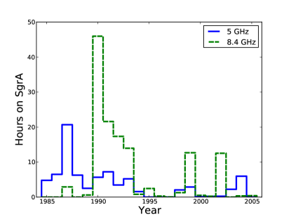
Figure 1.— Integration time on Sgr A*  in 5 GHz and 8.4 GHz observations per year from 1985 to 2005.

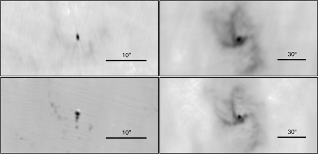
Figure 2.— Pipeline-generated images of Sgr A*. Displayed images have the median image rms value among all images with the same frequency and configuration. Images are scaled by a square-root transfer function. Upper left: 5 GHz dataset in A configuration. Upper right: 5 GHz dataset in CnB configuration. Lower left: 8.4 GHz dataset in A configuration. Bottom right: 8.4 GHz dataset in CnB configuration. The imaged regions are centered on the same coordinates in this figure and North is up and East is left for each image.

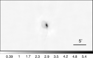
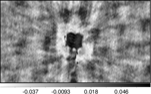
Figure 3.— A pipeline-calibrated image of Sgr A*  from a 5 GHz, D configuration data set (left) and its corresponding model-subtracted image (right). Note that while some structure remains in the model-subtracted image of Sgr A*, the amplitude of the residual structure is roughly 1% that of the unsubtracted image. The grey scale is in units of ${\rm Jy\,beam^{-1}}$.

The VLA operates in configurations labeled from A to D, where A configuration has the highest resolution and D configuration is most sensitive to extended structure. The VLA also adopts hybrid configurations (DnC, CnB, BnA) that deploy an extended North arm to optimize observations of sources at lower declination. Our data spans all configurations of the VLA. At both 5 GHz and 8.4 GHz, the majority of observation time was in A, BnA, or CnB configuration, providing relatively high angular resolution. Higher resolution datasets require more processing for the same field of view due to the larger number of pixels. Instead of imaging the full primary beam (half-power widths of $9{}^{\prime}$ and $5.4{}^{\prime}$ at 5 and 8 GHz, respectively), we adopted a resolution-dependent field of view that kept fixed the number of pixels, resulting in a minimum area coverage of $72\arcsec\times 72\arcsec$ in A configuration. This requirement guarantees that the most interesting regions of the Galactic center including the nuclear star cluster, the disk of young massive stars, and the Hii region Sgr A West are all included in every image. Since all but one potential radio transient investigated in datasets with larger fields of view were located within this minimum area, the restriction seems justified in retrospect.

2.2. Finding Radio Transients

Using the Common Astronomy Software Applications (CASA; McMullin et al., 2007) package, we have developed an automated data reduction pipeline to process each observation and search for variability on timescales from 30 seconds to about five minutes. While most transient surveys look for variability across independent observations, we look for variability within observations using a CLEAN model subtraction method outlined in Chatterjee et al. (2005).

Table 2RMS statistics of pipeline-generated 10 s residual images

Frequency	VLA Configuration	Median RMS	Mode RMS	90% Interval of RMS Values
(GHz)		$({\rm mJy\,beam^{-1}})$	$({\rm mJy\,beam^{-1}})$	$({\rm mJy\,beam^{-1}})$
5	A	8.1	7.0	2.4 – 15.6
	BnA	19.4	10.7	3.7 – 34.1
	B	18.6	17.2	8.9 – 36.2
	CnB	21.8	21.7	13.4 – 43.1
	C	31.1	31.0	21.4 – 42.7
	DnC	52.7	46.4	35.6 – 93.6
	D	49.8	50.8	17.5 – 112.7
8.4	A	6.4	5.0	2.3 – 15.6
	BnA	11.1	6.8	4.8 – 32.3
	B	10.5	7.8	5.7 – 17.0
	CnB	18.8	12.6	10.4 – 48.5
	C	18.3	10.8	10.8 – 56.4
	DnC	31.7	19.1	18.5 – 52.5
	D	71.8	27.7	10.1 – 211.9

Note. — The mean, median, and 90% interval of RMS values of 10 s residual images are shown. Cases of extremely low RMS values were excluded from the statistics as potential amplitude mis-calibrations

2.2.1 Flagging, Calibration, and Imaging

For each observation, the data are flagged to remove corruption from RFI, calibrated using the available flux and phase calibrators, then imaged using CLEAN deconvolution. Though the specific parameters may change for different observing frequencies and array configurations, the basic data reduction procedure is as follows.

First, the data set for an observation is retrieved from the NRAO Data Archive. Before the data can be calibrated, we run an automated RFI flagging routine using the TFCrop algorithm in the CASA task flagdata. TFCrop is able to identify RFI in an uncalibrated data set by fitting a piecewise third-order polynomial to the time-averaged bandpass of subintervals of data collected on each baseline. The data set is flattened by dividing by the average bandshape for each of the considered subintervals. RFI is identified as outlier data in either time or frequency. In addition to RFI flagging, the first 20 seconds of each scan is flagged to remove any data taken as the telescope was settling after slewing back from a calibrator source.

After flagging, the data are calibrated using both the standard gain calibration procedures and several rounds of self-calibration on Sgr A*. For complex gain calibration, solutions are determined using the calibrator sources provided in each observation. After gain calibration, the data are self-calibrated using Sgr A* itself as a calibrator. To do this, we image the visibility data using the Cotton-Schwab implementation of the CLEAN deconvolution algorithm (Schwab, 1984) with natural weighting of the visibility data. The deconvolution produces a model of the data that is used as the calibrator model in the next iteration of self-calibration. Two iterations of phase-only self-calibration are performed, followed by one iteration of phase and amplitude self-calibration. The result of this process is full-observation model of Sgr A* and a deconvolved image.

Once a model image has been generated for a full observation, the model is Fourier transformed and subtracted from the calibrated visibility data. The resulting model-subtracted visibility data is imaged on shorter intervals to search for transient events. Since one of the fundamental assumptions in interferometric imaging is that the sky intensity distribution is constant over the observing span, the generated CLEAN model will essentially be the time-averaged intensity distribution. Radio transients that last for a small fraction of the observing time will only lose a small fraction of their flux to the model. However, if a radio transient lasts for a large fraction of the observing time, it will have most of its flux contained in the model and be difficult to detect once the model is removed. As a result, our transient search will be limited to events with durations much shorter than the full observing span or events that are sufficiently faint to avoid being included in the CLEAN model.

A few typical images of the Galactic center produced by the processing pipeline are illustrated in Figure 2, and an example images of the Galactic center before and after model subtraction are shown in Figure 3.

Table 3A summary of the candidate events

Name	Freq	VLA	Duration	$\Delta$RA	$\Delta$Dec	$\delta\theta_{\rm{Sgr~{}A*}}$	Int. Flux†	Peak Flux
	(GHz)	Config	(seconds)	(sec)	(arcsec)	(arcsec)	(mJy)	$({\rm mJy\,beam^{-1}})$
Level 2
RT 850630	5	CnB	120	40.00(2)	$-$23.6(2)	4.69(21)	456 $\pm$ 42	149 $\pm$ 26
RT 910627	8.4	A	100	38.8578(9)	$-$19.34(2)	18.09(2)	180 $\pm$ 21	100 $\pm$ 11
Level 1
RT 910817	8.4	A	60	40.059(2)	$-$26.96(4)	1.24(4)	115 $\pm$ 17	72 $\pm$ 7
RT 950721	8.4	A	60	40.0469(9)	$-$28.35(3)	0.23(2)	36 $\pm$ 3	55 $\pm$ 5
RT 921210	8.4	A	480	40.048(1)	$-$28.30(4)	0.18(3)	33 $\pm$ 5	44 $\pm$ 6
RT 920208	8.4	CnB	140	40.13(1)	$-$26.9(2)	1.56(15)	100 $\pm$ 12	86 $\pm$ 10
RT 860417	5	A	50	40.582(4)	$-$22.36(9)	8.99(7)	180 $\pm$ 30	47 $\pm$ 8
RT 871129	5	B	150	39.592(4)	$-$85.1(1)	57.23(13)	308 $\pm$ 24	92 $\pm$ 7
Level 0
RT 910912	8.4	A	150	41.8284(6)	$-$32.87(2)	23.66(1)	162 $\pm$ 8	192 $\pm$ 10
RT 930109	8.4	A	180	39.6448(4)	$-$17.45(1)	12.05 (1)	116 $\pm$ 4	99 $\pm$ 4
RT 900704	8.4	BnA	340	40.092(7)	$-$27.2(1)	1.05(11)	85 $\pm$ 14	119 $\pm$ 19
RT 911125	8.4	BnA	120	40.019(5)	$-$27.5(1)	0.86(9)	58 $\pm$ 10	80 $\pm$ 13
RT 900914	8.4	B	70	39.951(7)	$-$29.8(2)	2.12(13)	117 $\pm$ 13	172 $\pm$ 20
RT 870814	5	A	120	37.544(1)	$-$22.22(3)	33.54(2)	91 $\pm$ 5	75 $\pm$ 4
RT 871026	5	BnA	70	39.996(4)	$-$28.00(6)	0.87(5)	40 $\pm$ 3	54 $\pm$ 5
RT 871030	5	BnA	120	39.994(4)	$-$27.63(5)	1.04(5)	177 $\pm$ 13	239 $\pm$ 17

Note. — The top block contains the candidate events that thoroughly passed all tests and had smooth light curves in the event region throughout the observation (Level 2 candidates). The second block contains candidate events that have passed all tests (the sixth column in Table 1), but did not have smooth light curves over their respective observation (Level 1 candidates). The bottom block contains the potential events from A, BnA, and B configurations that either barely failed a test or did not receive the full array of tests (ie. had only one polarization; Level 0 candidates). The transients are named for the UTC date on which they occurred in the form RT YYMMDD. The duration is the time from the appearance of the transient signal to the disappearance, regardless of whether the emission was above the cutoff threshold at all times. The positions ($\Delta$RA, $\Delta$DEC) are measured as offsets from ${\rm 17^{h}45^{m}00^{s}}$ and $-29^{\circ}00^{\prime}00^{\prime\prime}$. The distance ($\delta\theta$) is measured from Sgr A*  at RA = ${\rm 17^{h}45^{m}40.06^{s}}$, DEC = $-29^{\circ}00\arcmin 28\farcs 20$. The integrated and peak flux densities in the last two columns are reported for the maximum of the transient events. Positions and integrated flux densities are derived using the imfit routine in CASA, which fits 2D gaussians to input sources assuming a gaussian noise background. The local rms around each transient is propagated to account for uncertainties from the undulating background. Because the fitting routine assumes uncorrelated noise, the uncertainties are almost certainly underestimated.
^† The integrated flux is discrepant from the peak flux density due to insufficient model subtraction and sparse u-v coverage. We assume the peak flux density when calculating rates and speculating on source classes.

In searching for transient events, we have chosen to model the background flux for each observation instead of creating a global model from all the available data in the archive. A global model would provide a higher fidelity representation of the flux in the region (as a result of much better u-v coverage) and would be sensitive to the long-duration transients ($\Delta t_{\rm dur}\gtrsim T_{\rm obs}$) that get missed when averaged into a single observation model. However, the residual images created from subtracting a global model could have errors in the cross-calibrations between different observations, introducing artifacts like constant offsets to the residual images. Our search is targeted at transients with durations less than a few minutes (which accounts for a small fraction of the integration time in almost all observations), and so we have chosen the observation-based modeling approach to potentially avoid cross-calibration complications.

2.2.2 Identifying Transient Events

After removal of the full observation model, the model-subtracted visibility data is imaged without CLEANing in intervals of one, two, and six times the visibility sample time (typically 10 s, but could also be 20 s or 30 s). For each observation of Sgr A*, the mean, root-mean-square (rms), maximum, and minimum values of each image are calculated as a function of time in order to locate and track temporal variations in flux density. Excursions of typically 2 or 3 standard deviations in the maxima between consecutive images are noted as potential transients, which usually corresponded to peak excursions of about seven times the image rms.

The potential transients are then inspected by eye in the residual images to ensure that events are physically plausible and not spatially dispersed or moving in the image domain. Additionally, the five brightest pixels in all images are identified and small regions around these pixels are tracked over all scans in the observation. This process isolates potential candidates and excludes from further consideration regions that have a constant excess in flux density due to insufficient CLEANing of the full observation model. Since events have to occur with statistical significance at the same location in consecutive 10 s images to resolve a rise and fall, this search is sensitive to transients with timescales down to about 30 s.

As a result of the short integration times and complex structure present in the Galactic center, the residual images produced from the model-subtracted visibility data are contaminated with large-scale ripples and sidelobes. In an attempt to avoid spurious detections, we set a fairly high threshold for identifying a potential transient candidate (typically six to seven times the image rms). The distribution of image rms values for all of the 10 s residual images made from the 8 GHz A-configuration data is shown in Figure 4 and a breakdown of values by frequency and configuration is presented in Table 2. In addition to false-positives from noise, imaging surveys for radio transients must also guard against more subtle imaging artifacts. The careful reanalysis by Frail et al. (2012) of an archival VLA transient survey by Bower et al. (2007) found that many of the claimed detections were actually imaging artifacts created by insufficient CLEANing, imperfect calibration of the data, or other subtle antenna- or baseline-based errors. To filter out false-positives from such effects, we adopt a rigorous series of confirmation tests for each potential transient candidate. Candidates that failed at least one of these tests or did not receive the full suite of tests will be referred to as Level 0 candidates. Candidates that passed all tests will be referred to as Level 1 candidates, and candidates that are particularly promising will be referred to as Level 2 candidates.

2.2.3 Event Confirmation

After observations containing potential candidates events are identified, they are re-analyzed using subsets of the data in an attempt to reject false-positives caused by imaging artifacts or RFI. A failure to detect the transient in the same location with comparable flux densities in all subsets will result in the rejection of the candidate event. Candidate events that passed all these tests (Level 1 and 2 events) are listed in the top two blocks of Table 3. In the first test, the full observation is split into two polarizations (right/left circular polarization) and separately run through the imaging and processing pipeline. Though this test may reject real circularly polarized astrophysical sources, it will also effectively remove certain types of RFI.

Figure 4.— A histogram of the rms values for 10 s residual images from all 8 GHz observations of the Galactic center in A configuration. The histogram is roughly Gaussian with a peak rms of $5~{}{\rm mJy~{}beam}^{-1}$. The extended tail towards higher rms values represent datasets that were either miscalibrated or improperly flagged. The expected thermal noise rms for 8 GHz observations in A configuration is approximately 0.5 mJy. Due to sidelobe effects and unsubtracted structure, our distribution of rms values has a median of 6.4 mJy.

In the second test, the full observation is imaged separately in each of the two intermediate-frequency (IF) bands processed by the VLA. For almost all of the observations considered in this archival search, the difference in center frequencies between the two IFs is ${\leq}100~{}\rm MHz$. Thus, the detection of a transient event in one band but not the other would indicate that the source is either a broadband source with an extremely steep spectrum, a source with narrow line-like emission, or (most probably) narrow-band RFI.

In the final test, the data are split into different subarrays and re-imaged to test for corruption by a bad antenna or baseline. The simplest way to isolate a single bad antenna is to create two disjoint sets of antennas with similar u-v coverage. However, the reduction of sensitivity in this case is enough to make detection of any of the transient events difficult. To reclaim some of the lost sensitivity, the antennas are instead split into three groups of 18 antennas where each group has some overlap with the others, but each antenna is absent from one of the groups. Detecting the candidate in all three antenna groups means that the transient could not be the result of a single bad antenna or a single bad baseline.

The results of the confirmation tests are summarized in Table 3. Level 1 and 2 candidates are listed in the first two blocks of Table 3. While Level 1 candidates passed all our confirmation tests, their light-curves behaved erratically over the observation, suggesting they may potentially be a processing artifact. The first block contains the two highest quality candidates (Level 2) that passed all the tests and had a smooth, well-behaved lightcurve. The third block of Table 3 contains Level 0 candidates in the most extended array configurations that either could not have the full suite of tests run (e.g., only one polarization), or marginally failed one of the tests.

2.2.4 False Positive Rate

As one final check on our candidate events, we can estimate the false positive rate expected for the transient search. For each configuration and frequency, the number of independent samples in an image is roughly the number of synthesized beams in that image, $N_{\rm b}\sim(\theta_{\rm FOV}/\theta_{\rm beam})^{2}$. If snapshot images are made with duration $\Delta t$, then the total number of independent samples in a data set with $T_{\rm obs}$ of total observing time is $N=N_{\rm b}\times(T_{\rm obs}/\Delta t)\approx 3.7\times 10^{9}$. We note that this rough estimate does not account for sidelobes and other unmodeled structure that are correlated across residual images. Phase errors from atmospheric delays and instrumental errors could also potentially lead to enhancements of signal. We do find that the distribution of changes in pixel values from one residual image to the next is roughly Gaussian, with systematic sidelobe structure varying on longer timescales than the transients we detect. We search for excursions that are localized in time and position on the sky, and note when transients are in regions of high sidelobe activity to minimize the effect of unmodeled structure.

Assuming the noise in each of the residual images is roughly Gaussian, with the parameters of the Gaussian varying between images, we expect $N_{\rm FP}(S\geq 5.8\,\sigma)=12$ false positives with significance at or above the $5.8\,\sigma$ level set by the weakest event detected in our search. This rough estimate also does not include the requirement that events occur in a single location in consecutive snapshots (which would dramatically reduce the false positive rate), nor does it explicitly account for the effects of unmodeled structure (which artificially increase the $\sigma$ parameter in each of our residual images). However, it provides a useful comparison to the 23 Level 0, Level 1, and Level 2 candidates produced by the detection pipeline. Since only two of these events are classified as Level 2 candidates, it is likely that the false positives are largely accounted for by our confirmation tests.

3. Results

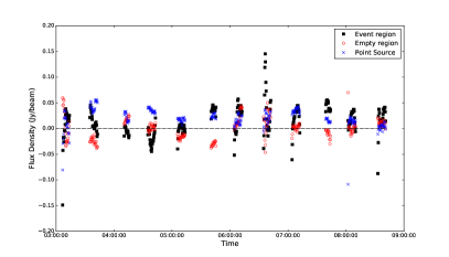
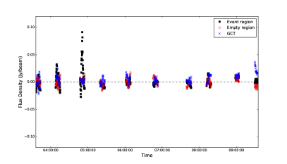
Figure 5.— Plots of the peak flux density of the burst vs. time for RT 850630 in 20 s cadences (left) and RT 910627 in 10 s cadences (right) in model-subtracted images. The black squares correspond to the flux density of the event over the duration of observation, red points are the flux density of an empty region during the event, and blue points are the flux density a reference source in each field, plotted for comparison. Gaps in the light curves are largely due to time on other fields

. All times and dates are in UTC.

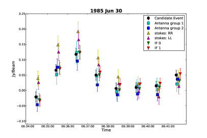
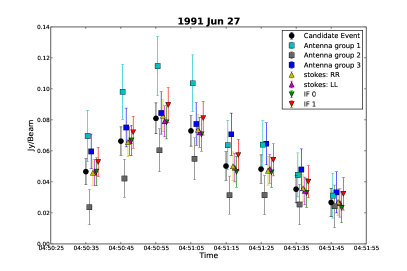
Figure 6.— Left: light curves for RT 850630 in 60 s residual images for different groupings of data: data split by spectral windows, data split by stokes parameters (LL, RR), and finally, data split between two antenna groups. The light curves labeled by each symbol are offset by 5s of each other for clarity. Right: light curves for RT 910627 in 10 s residual images for different groupings of data: data split by spectral windows, data split by stokes parameters (LL, RR), and finally, data split between three antenna groups such that each antenna is missing in at least 1 group. The light curves labeled by each symbol are offset by 0.5 s for clarity. Error bars correspond to the rms of the residual image. All times and dates are in UTC.

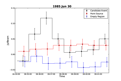
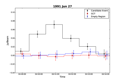
Figure 7.— Left: light curves of RT 850630, a compact source, and an empty region in the Sgr A*  field from 60 s residual images. Right: light curves of RT 910627, the GCT, and an empty region in the Sgr A*  field from 60 s residual images. Both bursts occur with no corresponding excursions in the compact source for RT 850630, the GCT for RT 910627, or the empty region. Error bars correspond to the rms of the residual image. All times and dates are in UTC.

3.1. Candidate Events

Of the 23 candidate transient events identified in our processing and detection pipeline, only eight passed all of the confirmation tests designed to filter out RFI and imaging artifacts. The locations of these candidates relative to Sgr A* are displayed in Figure 14. Of the eight Level 1 candidates, only two are deemed to be Level 2 candidates based on the smoothness of their lightcurves (Figure 5). We note that while many of our candidate events appear to be resolved, this is mainly due to excess flux from improper model subtraction, noise, and PSF-related effects (Figures 10 and 11). In this section, we present details on these two events, and discuss efforts to find counterparts at other wavelengths.

3.1.1 RT 850630

RT 850630 was detected in project AY8, observed on 1985 June 30 at 5 GHz. The event lasted roughly 120 s, was located $4\farcs 6\pm 1\farcs 9$ north of Sgr A*, and had a maximum peak flux density of $149\pm 26~{}{\rm mJy\,beam^{-1}}$.

We split the data from project AY8 into different subgroups (by frequency, sub-array, and polarization) and found a consistent transient signal in each subgroup, as shown in Figure 6. Further, we constructed light curves of an empty sky region anti-symmetric to the event with respect to the pointing center, as well as a point-like test source composed of the two objects 1LC 359.985+0.027 and 2LC 359.985+0.027 (RA${\rm=17^{h}45^{m}28.66^{s}}$ Dec = –$28^{\circ}56\arcmin 03\farcs 943$) in the same field (Lazio & Cordes, 1998a), in case the entire residual image had an artificially elevated flux for a brief period of time. As shown in Figure 7, only the event region showed a rise in flux density. Our measured peak flux density of 143 mJy for the point-like test source is in agreement with the 5 GHz peak flux density reported for the object by Becker et al. (1994). Due to the proximity of RT 850630  to Sgr A*, we are unable to meaningfully constrain its quiescent emission even with our deepest images of the Galactic center. We find no matches to known radio sources in the Master Radio Catalog from the High Energy Astrophysics Science Archive Research Center (HEASARC) archives.

Since the residual visibilities are imaged on short timescales, each image has only snapshot u-v coverage, and incompletely subtracted structure around Sgr A* produces large sidelobes. As such, there is a risk that in spite of our tests, RT 850630 is an artifact. Furthermore, RT 850630 appears in a region of high residual image flux due to poor model subtraction (Figure 8). In Figure 10, we verify that the dominant side lobe pattern at the location of the transient event is traced by the PSF. Thus, the sidelobe pattern in the residual image was probably produced by the transient event itself, although we cannot definitively rule out an imaging artifact. We also generated 20 s images of the two minutes of transient activity without prior model-subtraction and detected a flux increase comparable to the flux of RT 850630. Finally, we conducted an independent re-analysis of the data using the AIPS software package and detected the transient at the same location and time in project AY8.

3.1.2 RT 910627

RT 910627 (see Figure 9) was detected in project AZ52, observed on 1991 June 27 at 8.4 GHz. It lasted roughly 100 s, was located roughly 20″ northwest of Sgr A*, and had an maximum peak flux of $100\pm 11~{}{\rm mJy\,beam^{-1}}$. We estimate that the effect of bandwidth smearing amounts to roughly a 10% decrease in peak flux density, based on the equations for bandwidth smearing in Bridle & Schwab (1999), for which our reported measurement is not corrected. We also find no matches to known radio sources in the Master Radio Catalog from the HEASARC archives.

RT 910627 passed all tests for validity and survived each step of the additional analysis as described above for RT 850630, using the long-duration galactic center transient (hereafter GCT) detected by Zhao et al. (1992) as a substitute for a constant point-like source to construct additional light curves. The quiescent emission of the candidate event can be constrained to be $\lesssim 1$ mJy/beam based on the flux of the event region in the image of the full observation. We find that this event appears to be split into two statistically insignificant sources if imaged without self-calibration, and this event is not detected after reducing the data with the AIPS software package. However, we performed an additional independent re-analysis of the data set using the CASA software package and detected the transient at the same location and time as the pipeline. For the above reasons, this event remains more suspect as an imaging artifact than RT 850630.

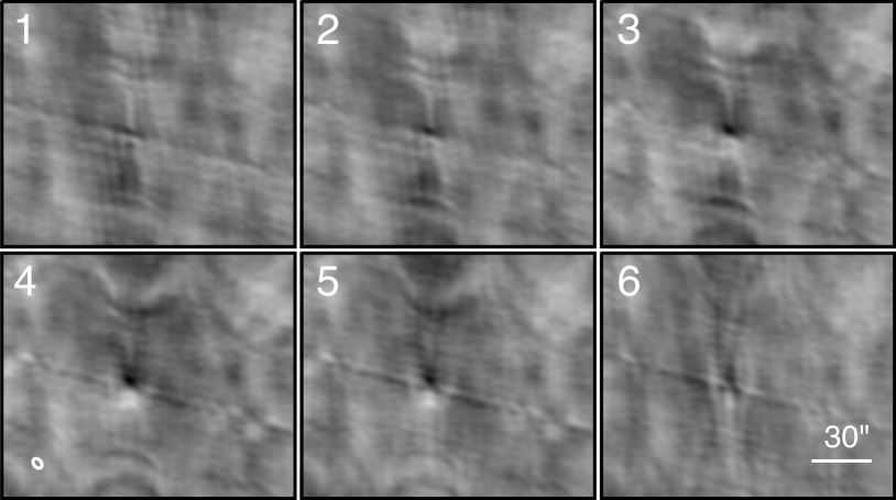
Figure 8.— 20 s residual images corresponding to RT 850630, with the greyscale ranging from $-0.15~{}{\rm mJy~{}beam}^{-1}$ to $0.15~{}{\rm mJy~{}beam}^{-1}$ and linear scaling. The images span UTC 6:35:25 to 6:37:25 on June 30, 1985. Each snapshot image is produced with u-v data from which a model for Sgr A*  has already been subtracted. The region of negative flux below RT 850630 has a peak amplitude amplitude $\sim 60\%$ as large as the peak amplitude of RT 850630. A uniform amplitude scale has been applied to each image, and the beam is shown in the lower left of the figure. North is up and East is left. Each panel of this figure is available as the Data behind the Figure.

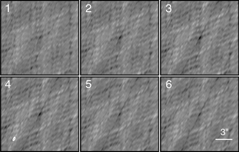
Figure 9.— 10 s residual images corresponding to RT 910627, with the greyscale ranging from $-0.095~{}{\rm mJy\,beam}^{-1}$ to $+0.095~{}{\rm mJy\,beam}^{-1}$ and linear scaling. The images span UTC 4:50:35 to 4:51:35 on June 27, 1991. See caption for Figure 8. Each panel of this figure, after a primary beam correction, is available as the Data behind the Figure.

3.2. Counterparts at Other Wavelengths

Given the dates and locations of the two best candidate events, we can look for potential counterparts at other wavelengths. First, we check to see if our events are consistent with any known transients in the Galactic center. None of the events are coincident with the GCT (Zhao et al., 1992), the magnetar J1745$-$2900, or any of the transient X-ray binaries discovered by Muno et al. (2005b). See Figure 14 for a visual overview of the region.

Next, we compare our events against known X-ray and near-infrared (NIR) point sources. The 2 Ms Chandra point source catalog of Muno et al. (2009) contains 63 X-ray sources within 25″ (1 pc at 8.5 kpc) of Sgr A*. One of these sources, CXOGC 174540.1$-$290025, is $2\farcs 6$ from RT 850630, falling just inside the synthesized beam of that observation. Interestingly, CXOGC 174540.1$-$290025 is characterized by Muno et al. (2009) as having short-term variability. However, given the number of sources, the probability of getting at least one source within the relatively large synthesized beam of RT 850630 is about $0.985$, so not much significance can be attached to this association. RT 910627, which is much better localized and further from Sgr A* than RT 850630, has no associated X-ray point source.

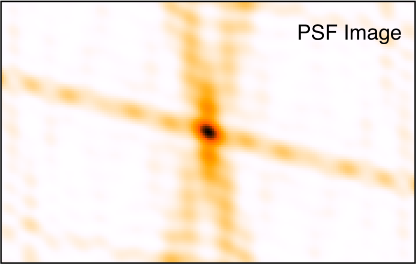
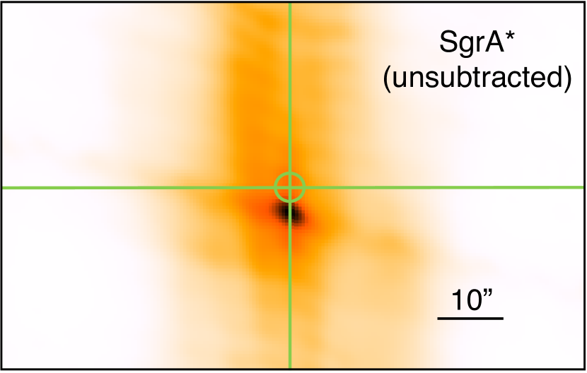
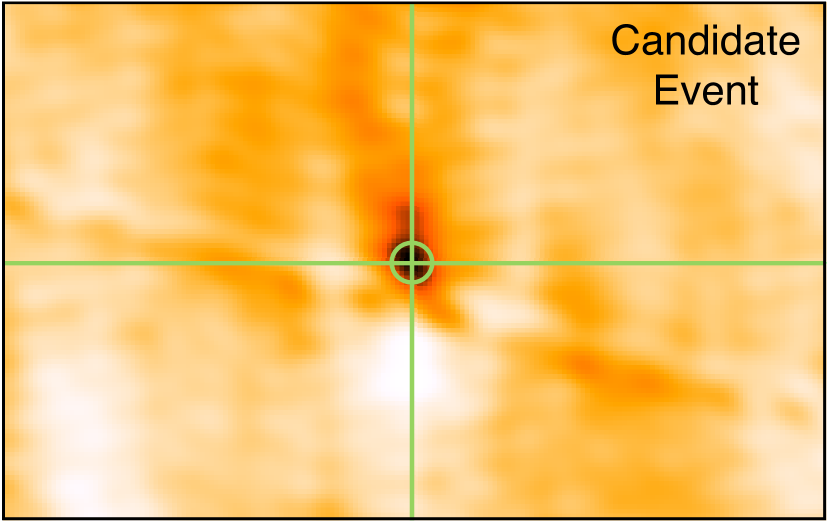
Figure 10.— Left: The point spread function Center: An image of Sgr A*  centered on RT 850630in the 60 s time bin corresponding to the peak of RT 850630. Right: 60 s image with Sgr A*  model subtraction, showing RT 850630. The vertical side lobe pattern at the location of RT 850630 is traced by the PSF.

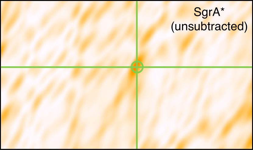
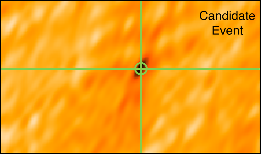
Figure 11.— Left: The point spread function Center: An image of Sgr A*  centered on RT 910627in the 10 s time bin corresponding to the peak of RT 910627. Right: 10 s image with Sgr A*  model subtraction, showing RT 910627. The side lobe pattern at the location of RT 910627 is traced by the PSF.

Using the Schödel et al. (2009) catalog of the positions and proper motions of over 6000 stars within a projected distance of 1 pc from Sgr A*, counterparts to the transient events can be sought in the NIR. Given the high density of sources and the large synthesized beam, any association with RT 850630 is difficult to determine. However, one of the ${\sim}100$ sources within the synthesized beam is the bright M1 supergiant GCIRS 7. There is only one source within the beam of RT 910627. Given the size of the beam and the number of sources in the region, the probability of a chance overlap is about $0.63$, so the association is again tenuous.

Finally, the dates and times of the candidate radio transients can be checked against known gamma-ray burst (GRB) catalogues. There are no reported GRBs coincident with RT 850630, although at the time the only operational gamma-ray detector was the Pioneer Venus Orbiter (Klebesadel et al., 1980; Evans et al., 1981). GRB 910627 occurred at UT 04:29:23 on 1991 Jun 27, about twenty minutes before RT 910627. However, the position of GRB 910627 is constrained to an error box of about one degree centered on ($\alpha=13^{\rm h}17^{\rm m}29^{\rm s}$, $\delta=02^{\circ}30\arcmin 27\arcsec$), which rules out any possible origin near the Galactic center (Hurley et al., 2000).

The lack of clear counterparts to our transient events at other wavelengths is not surprising since these events occurred undetected 25 to 30 years ago (1985 and 1991). There were no targeted efforts at followup, and no contemporaneous programs with regular observations of the Galactic center. Repeating the present analysis on recent observations with good multiwavelength coverage (e.g., the recent G2 campaign; see Gillessen et al., 2013) might permit the identification of counterparts to detected transient events.

4. Occurence Rate of Transient Sources

Assuming our top two candidates are real astrophysical transients, we can estimate the rate of occurrence of similar events as a function of peak flux density. We provide two different types of rates here: the transient rate ($\rho$, events per unit time and solid angle) and the Galactic center rate ($r$, events per unit time). The transient rate is the standard rate that accounts for the variable sky coverage for each observation and can be easily compared against similar rates for other transient sources. The Galactic center rate, however, is useful if the population of potential transient events is entirely contained within the solid angle of the smallest image used in this survey, as is likely if the sources are associated with the Galactic center.

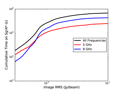
Figure 12.— The cumulative integration time on Sgr A*  from all images that have a lower rms than the abscissa value.

4.1. Transient Rate

Table 4Areas Surveyed and Time on Sgr A*  for given Sensitivities

Image RMS	Epochs∗	Area Surveyed	Time† on Sgr A*
(mJy)		(deg2)	(hr)
$\leq$ 5	4 098	19.9	13.5
$\leq$ 10	25 812	37.1	74.1
$\leq$ 20	45 713	73.6	131.7
$\leq$ 50	59 530	138.0	176.8
$\leq$ 100	62 602	166.5	189.8
$\leq$ 200	64 419	176.9	196.1
$\leq$ 500	64 856	178.6	197.4

Note. — Column 1 is the rms of an image; column 2 is the number of residual images that satisfy the image rms criteria; column 3 is the cumulative number of square degrees that an equivalent number of 10 s images would produce; column 4 is the cumulative time on Sgr A*.

^∗ An Epoch refers to a 10 s, 20 s, or 30 s image, as determined by sample time of the visibility data.

^† The time on Sgr A*  does not approach the stated 214 hours of observation time due to RFI flagging.

The transient rate, $\rho$, which is just the number of detectable transients per unit solid angle and time, can be inferred from the observed number of transients in the analyzed VLA data set. If we let $\Omega_{i}=\Omega_{A,i}\,\Delta t_{i}$ be the product of the solid angle ($\Omega_{A,i}$) and duration ($\Delta t_{i}$) of a single snapshot, then the total volume of the survey is just $\Omega=\sum_{i}\Omega_{i}$. If we assume that the number of transients occuring in any given volume element is Poisson distributed, then the probability distribution for the number of observed transients is given by

$$P\left(n=k~{}|~{}\rho,\mathcal{I}\right)=\frac{\left(\rho\Omega\right)^{k}e^{-\rho\Omega}}{k!}$$ (1)

where $n$ is the number of transients detected in some volume $\Omega$, $\rho$ is the transient rate, and $\mathcal{I}$ encapsulates all other prior information (including the fact that the counts follow a Poisson distribution). Using Bayes’ theorem, Equation 1 can be inverted to find the probability distribution for the transient rate given the observed counts:

$$P(\rho~{}|~{}n=k,\mathcal{I})=\frac{P(n=k~{}|~{}\rho,\mathcal{I})P(\rho~{}|~{}\mathcal{I})}{P(n=k~{}|~{}\mathcal{I})}.$$ (2)

Adopting a uniform prior on the rate, so that $\rho\in\left[0,\rho_{\rm u}\right]$ with some large upper limit given by $\rho_{\rm u}$, we find that

$$P(\rho~{}|~{}n=k,\mathcal{I})=\frac{\Omega\left(\rho\Omega\right)^{k}e^{-\rho\Omega}}{k!}\,.$$ (3)

Though not expressed explicitly in Equation 3, the number of events observed (and thus the rate inferred) is dependent upon the event detection threshold. The detection threshold for snapshot image $i$ is roughly $S_{{\rm min},i}=7\sigma_{{\rm rms},i}$, where $\sigma_{{\rm rms},i}$ is the rms noise level in the image. Since an event is only detectable if its peak flux density exceeds the detection threshold, it is necessary to calculate the rate as a function of $S_{\rm min}$. The above-threshold event rate $r(S_{\rm min})$ can be calculated with Equation 3 using the number of events $n(S_{\rm min})$ in a volume $\Omega(S_{\rm min})$ for all snapshot images with $S_{{\rm min},i}\leq S_{\rm min}$. A summary of the areas surveyed and time on Sgr A*for given sensitivities is provided in Table 4, and the cumulative integration time on Sgr A*as a function of image rms is plotted in Figure 12.

Given the observed values for $n(S_{\rm min})$ and $\Omega(S_{\rm min})$, we can infer $\rho(S_{\rm min})$ to be the maximum likelihood value of Equation 3 with an uncertainty set by the most compact range containing 95% of the posterior distribution. For a detection threshold of $S_{\rm min}=94~{}\rm mJy$, corresponding to the highest threshold at which both events are detectable, we observe two events in $\Omega(94~{}\rm mJy)=0.14~{}{\rm hr\,deg}^{2}$, giving a rate of $\rho(n{=}2,\,S_{\rm min}{=}94~{}\rm mJy)=14^{+32}_{-12}~{}{\rm hr}^{-1}\,{\rm deg}^{-2}$. Similarly, for a detection threshold of $S_{\rm min}=149~{}\rm mJy$, where only RT 850630 is detectable, we observe one event in $\Omega(149~{}\rm mJy)=0.22~{}{\rm hr\,deg}^{2}$, giving a rate of $\rho(n{=}1,\,S_{\rm min}{=}149~{}\rm mJy)=5^{+17}_{-4.8}~{}{\rm hr}^{-1}\,{\rm deg}^{-2}$.

Finally, since it is still possible that both of these events could be RFI and imaging artifacts, the 95% upper limits for the rates with no detections are calculated and shown as a function of detection threshold in Figure 13.

4.2. Galactic Center Rate

If the transient events arise from a source population around Sgr A* that is entirely contained within the smallest image of our survey, then there is no longer any solid angle dependence on the rate. In such a case, the most natural rate is one of events per unit time, which we will call the Galactic center rate, $r$. Following Section 4.1, the posterior for the Galactic center rate is

$$P(r~{}|~{}n=k,\mathcal{I})=\frac{T\left(rT\right)^{k}e^{-rT}}{k!}\,.$$ (4)

where $n$ is the number of transients detected in some time $T$.

For a detection threshold of $S_{\rm min}=94~{}\rm mJy$, we observe two events in $T(94~{}\rm mJy)=4.30~{}{\rm days}$, giving a rate of $r(n{=}2,\,S_{\rm min}{=}94~{}\rm mJy)=0.47^{+0.53}_{-0.27}~{}{\rm day}^{-1}$. Similarly, for detection thresholds of $S_{\rm min}=149~{}\rm mJy$, where only RT 850630 is detectable, we observe one event in $T(149~{}\rm mJy)=5.66~{}{\rm days}$, giving a rate of $r(n{=}1,\,S_{\rm min}{=}149~{}\rm mJy)=0.18^{+0.67}_{-0.17}~{}{\rm day}^{-1}$.

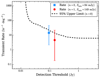
Figure 13.— The transient rates as a function of detection threshold (7 times the image rms) with error bars corresponding to the most compact 95% interval. The 95% upper limits in the case of no detections is shown as a dashed line. The point at 94 mJy corresponds to our detections of RT 850630 and RT 910627, as RT 910627 occurred at 94 mJy and RT 850630 (149 mJy) would have been detectable at that threshold. Similarly, the point at 149 mJy corresponds to the detection of RT 850630.

5. Astrophysical Source of Observed Events

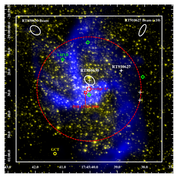
Figure 14.— The candidate events overlaid as white crosses on a map of the Galactic center with 8 GHz VLA data in blue and Hubble $1.9\mu\rm m$ data in yellow. The two most robust candidates are labeled with their transient identifier (RT 850630 and RT 910627). Candidate event 8 is located outside the field of view of this image. The white box is $70\arcsec\times 70\arcsec$ and the two red circles denote separations of $1\arcsec$ and $25\arcsec$ from Sgr A*. The positions of the magnetar J1745$-$2900, the GCT, and the LMXBs from Muno et al. (2005a) are all indicated. The beam sizes and orientations for RT 850630 and RT 910627(x10) are shown at the top of the image.

Transient radio signals can arise from both coherent and incoherent emission processes from a wide range of astrophysical objects including compact objects, stars, and planets (Cordes et al., 2004). Given the typical duration, flux density, and rate of our observed transient events, we can determine if they could feasibly originate from known astrophysical sources.

5.1. Coherent or Incoherent?

Radio emission can arise from both coherent and incoherent processes. Coherent emission (e.g., pulsar emission) typically results in steep spectra and a high degree of polarization, whereas incoherent radio emission (e.g., synchrotron radiation from jets) often produces spectra that are flat and wide-band with only moderate polarization. Theoretical estimates set the maximum brightness temperature of a synchrotron source to be $T_{\rm B}\sim 10^{11-12}~{}\rm K$ (Kellermann & Pauliny-Toth, 1969; Readhead, 1994), which we adopt as the upper limit for incoherent emission. Any source with $T_{\rm B}\gtrsim 10^{12}~{}\rm K$ must then arise from a coherent emission process.

The brightness temperature of a pulse is

$$T_{\rm B}=1.2\times 10^{13}~{}{\rm K}~{}\left(\frac{S_{\nu}}{100~{}{\rm mJy}}\right)\left(\frac{D}{8.5~{}{\rm kpc}}\right)^{2}\\ \times\left(\frac{\nu}{5~{}{\rm GHz}}\right)^{-2}\left(\frac{\Delta t_{\rm p}}{100~{}{\rm s}}\right)^{-2},$$ (5)

where $S_{\nu}$ is the peak flux density at frequency $\nu$, $\Delta t_{\rm p}$ is the characteristic width of the pulse, and $D$ is the distance to the source (Cordes et al., 2004).

For events like RT 850630  and RT 910627 ($S_{\nu}\sim 100~{}{\rm mJy}$, $\Delta t_{\rm p}\sim 100~{}{\rm s}$), the brightness temperature exceeds the threshold for incoherent emission if the source is at the Galactic center. However, the brightness temperatures for both sources can be reduced to $T_{\rm B}\lesssim 10^{12}~{}\rm K$ if they are foreground sources located $D\lesssim 2.5~{}\rm kpc$ from the Sun.

5.2. Galactic or Extragalactic?

Our survey was designed to target transient sources located near Sgr A*, but it is possible that the observed events originate from extragalactic sources or from nearby Galactic sources along the line of sight. If the sources are extragalactic, then they should occur isotropically on the sky. Extrapolating the inferred rate from Section 4.1 to the whole sky gives an event rate of $\rho_{\rm xgal}(S_{\rm min}{=}94~{}\rm mJy)=1.4^{+3.1}_{-1.2}\times 10^{7}~{}{\rm sky}^{-1}\,{\rm day}^{-1}$, which is incredibly high. For comparison, Fast Radio Burts (FRBs), a class of bright ($S_{\rm pk}\sim 1~{}\rm Jy$) short duration ($\Delta t\sim 1~{}\rm ms$) radio transients of presumed extragalactic origin occur at a rate of $\rho_{\rm FRB}\lesssim 7\times 10^{4}~{}{\rm sky}^{-1}\,{\rm day}^{-1}$ (Law et al., 2015). Even at the relatively unexplored timescales of $\Delta t\sim 100\,\rm s$, the existence of an undetected class of extragalactic radio transients occurring $\gtrsim 100$ times more frequently than FRBs seems unlikely. For the remainder of this analysis, we will only consider Galactic sources.

The source of the transient events, if real, are almost certainly Galactic. However, without the identification of a counterpart at some other wavelength, it is very difficult to determine if they are located near Sgr A* or are foreground sources seen along the line of sight. As a result, we will not exclude possible astrophysical sources on the basis of distance alone.

5.3. Pulsar Emission

The most obvious sources of radio transient emission are pulsars, which can exhibit variability over a wide range of timescales. Individual pulses typically have durations of ${\sim}1~{}\mu{\rm s}$ to ${\sim}100~{}{\rm ms}$ and vary in amplitude from pulse to pulse with each rotation of the pulsar. The emission can be sporadic as well, with nulling pulsars and RRATs sometimes emitting only a few observable pulses over many hours or days (McLaughlin et al., 2006). On longer timescales, the pulsar emission can be turned on and off for days or weeks at a time by large-scale changes to the magnetosphere (Kramer et al., 2006), and an otherwise consistent pulsar may have its observed flux density modulated by refractive and diffractive scintillation in the interstellar medium (Stinebring et al., 2000). Despite the diversity of variability, most pulsars would simply be too faint to account for our observed transient events. For all the pulsars in the ATNF Pulsar Catalog (Manchester et al., 2005) with reported flux densities and distances, the maximum 5 GHz flux density would only be about $1-10~{}{\rm mJy}$ if placed at the Galactic center. Though the transient events could not be caused by typical pulsar emission, it is possible that they could be the result of one or many giant pulses, like those observed in the Crab pulsar (B0531+21).

The Crab pulsar is a young ($\tau\approx 1~{}\rm kyr$) pulsar that frequently emits giant pulses, which are pulses with amplitudes at least ten times larger than the average. These pulses are incredibly bright, with observed peak flux densities as high as 2.2 MJy in less than $0.9~{}{\rm ns}$ (Hankins & Eilek, 2007). Much work has been done characterizing the Crab giant pulses, which seem to follow a power-law distribution in amplitude (Lundgren et al., 1995; Bhat et al., 2008; Majid et al., 2011; Mickaliger et al., 2012). Most studies report the index for the differential power-law amplitude distribution, $n(S)\propto S^{-\gamma}$, which gives the number of pulses within some amplitude bin. Measurements of the index range from $2\lesssim\gamma\lesssim 4$ for observing frequencies from $\nu_{\rm obs}=0.1-4~{}{\rm GHz}$ (Mickaliger et al., 2012, and reference therein). Since the intrinsic widths of Crab giant pulses can be smaller than the instrumental resolution, the observed peak flux density is often less than the intrinsic value. To avoid such complications, it is convenient to work with distributions of pulse fluence (often called the pulse energy), which is the time integrated flux density of the pulse. An additional benefit of using the pulse fluence instead of the amplitude is that the fluence is unaffected by scattering or other pulse shape distortions.

Majid et al. (2011) determined the cumulative fluence distribution of Crab giant pulses at 1.6 GHz and found that the rate of pulses with $E>E_{\rm p}$ goes roughly as $R(E>E_{\rm p})=R_{0}(E_{\rm p}/E_{0})^{-1.9}$ for $E_{\rm p}>5\times 10^{-3}~{}\rm Jy\,s$. From their Figure 9, we estimate $R_{0}\approx 3\times 10^{-3}~{}\rm s^{-1}$ for $E_{0}\approx 0.1~{}\rm Jy\,s$. The fluence of our RT 850630 is $E_{1}\sim\rm 0.1~{}Jy\times 100~{}s=10~{}Jy\,s$. Scaling this event with frequency and distance for comparison with the Crab gives

$$E_{\rm c,\nu_{0}}=E_{\rm gc,\nu}\left(\frac{\nu_{0}}{\nu}\right)^{\alpha}\left(\frac{d_{0}}{d_{\rm gc}}\right)^{-2}$$ (6)

where $d_{0}=2~{}\rm kpc$ is the distance to the Crab pulsar (Trimble, 1973), $\nu_{0}=1.6~{}\rm GHz$, $\alpha=-1.6$ is a typical pulsar spectral index (Lorimer et al., 1995), and $E_{\rm gc,\nu}$, $\nu$, and $d_{\rm gc}=8.5~{}\rm kpc$ are the fluence, frequency, and distance to a transient originating at the Galactic center. For RT 850630 ($E_{1}\sim 10~{}\rm Jy\,s$, $\nu=5~{}\rm GHz$), the scaled fluence is $E_{\rm c,\nu_{0},1}\sim 10^{3}~{}\rm Jy\,s$. Assuming the cumulative frequency relation from Majid et al. (2011) extends to these fluences, the expected rate of giant pulses from the Crab with $E>10^{3}~{}\rm Jy\,s$ is $R\approx 7\times 10^{-12}~{}{\rm s}^{-1}$, or about once every 4800 years. One event in 200 observing hours requires a population of ${\sim}1$ Crab-like pulsar at $330~{}\rm pc$, ${\sim}1000$ Crab-like pulsars at $2~{}\rm kpc$, or ${\sim}2\times 10^{5}$ Crab-like pulsars in the Galactic center. Such a large population is easily ruled out by previous multiwavelength constraints (Wharton et al., 2012).

5.4. Radio Flares from Dwarf Stars

Transient radio emission at GHz frequencies has also been seen in flares from dwarf stars. About 10% of the ${\sim}100$ observed dwarf stars with spectral types above M7 have some sort of radio activity (Berger, 2006). Most of the flares from late-type dwarf stars have peak 5 GHz flux densities around $S_{\rm pk}\lesssim 1~{}\rm mJy$ and durations of $\tau\gtrsim 10~{}{\rm min}$ (Berger, 2002, 2006; Hallinan et al., 2008). The largest flare of this type was seen in the M8 dwarf DENIS 1048$-$3956 and consisted of 5 minute long pulses at 4.8 GHz and 8.6 GHz with peak flux densities of $S_{4.8}\approx 6~{}\rm mJy$ and $S_{8.6}\approx 30~{}{\rm mJy}$, respectively (Burgasser & Putman, 2005). Several of the flaring ultracool dwarfs show ${\sim}100\%$ circularly polarized emission and are periodic on ${\sim}\rm hour$ timescales consistent with the rotational period of the star (Hallinan et al., 2007, 2008).

M-class dwarfs with spectral type below M7 also exhibit radio flaring and are much more active at other wavelengths than their later-type counterparts. Large flares with ${\sim}100\%$ circular polarization have been observed in both AD Leonis and DO Cephei with durations of $\tau\sim 1~{}{\rm min}$ and peak 5 GHz flux densities of $S_{\rm pk,5}\gtrsim 100~{}{\rm mJy}$ (White et al., 1989; Stepanov et al., 2001). Follow-up studies of AD Leo with larger bandwidth and higher time resolution have found that these flares are comprised of short ($\tau\sim 30~{}\rm ms$) subpulses with fractional bandwidths of $\Delta\nu/\nu\approx 5\%$ (Osten & Bastian, 2006, 2008).

The flares from active M dwarf stars like AD Leonis are a good match to our two best radio transient events in both peak flux density and observed duration ($S_{\rm pk}\sim 100~{}\rm mJy$, $\tau\sim 1~{}\rm min$). Though AD Leonis is one of the most luminous flaring M dwarf stars, it can only produce flares up to $S_{\rm max}\sim 1~{}\rm Jy$ at a distance of $d=4.9~{}\rm pc$. A similar star would result in flares comparable with our transient events ($S_{\rm pk}\sim 100~{}\rm mJy$) out to a distance of only $d\approx 16~{}\rm pc$. Adopting a local stellar mass density of $\rho_{\odot}=0.085\pm 0.010~{}M_{\odot}~{}{\rm pc}^{-3}$ (McMillan, 2011), the enclosed mass in our FOV ($\theta=70\arcsec$) is $M_{\star}\approx 10^{-5}M_{\odot}\,(d/16~{}\rm pc)^{3}$, which is significantly less than the typical M dwarf mass of $M\approx 0.075-0.5~{}\rm M_{\odot}$ (Lépine & Gaidos, 2011). Thus, it is unlikely that an M dwarf would be found along our line of sight to Sgr A*. Furthermore, our rejection of circularly polarized detections means our detections do not sharing the polarization properties of M dwarf star flaring activity.

5.5. GCRT J1745$-$3009

The Galactic center radio transient GCRT J1745$-$3009 (hereafter, GCRT) is an intermittently emitting source that has been detected by multiple observatories at 330 MHz (Hyman et al., 2005, 2006, 2007). Other radio transients had been detected near Sgr A*, but they were isolated events that lasted many months or years (Zhao et al., 1992; Bower et al., 2005). In contrast, the GCRT emits ${\sim}1~{}\rm Jy$ pulses at 330 MHz that last for about 10 minutes. The pulses repeat with a 77 minute period, though the emission duty cycle is only ${\sim}10\%$ (Hyman et al., 2005, 2006). The spectral index ($S\propto\nu^{\alpha}$) of the source is $\alpha=-4\pm 3$ (Hyman et al., 2006; Roy et al., 2010), but at least one burst was observed with a much steeper spectral index of $\alpha=-13.5\pm 3.0$ (Hyman et al., 2007). Though originally reported to have a very small polarized fraction, a recent reanalysis by Roy et al. (2010) found strong time-varying circular polarization in one GCRT burst. Follow-up searches in X-rays and near-infrared have produced no viable counterpart (Hyman et al., 2005; Kaplan et al., 2008).

The GCRT bursts are of comparable duration (${\sim}$minutes) and fluence ($E_{\rm p}\sim 10~{}\rm Jy\,s$ for $\alpha\approx-1.6$) to the observed transient events in our VLA sample. Like our candidate events, the GCRT has no known counterpart at other wavelengths. While a time-varying circular polarization and periodic nature of the emission are not seen in our events, all but one of the bursts from the GCRT have previously been detected with only upper limits on the circular polarization (Roy et al., 2010). Although it is certainly possible that there exists a GCRT-like source responsible for our reported transient events, the evidence to support this proposition is ambiguous.

5.6. X-Ray Binaries

X-ray binaries (XRBs) are yet another potential source of transient radio emission. The binaries are comprised of a neutron star or black hole and a low-mass (low-mass X-ray binaries; LMXBs) or high-mass (high-mass X-ray binaries; HMXBs) companion. Outflows from XRB jets can produce synchrotron radio emission, which can be transient during state transitions (Fender & Kuulkers, 2001). The radio outbursts can reach peak flux densities of $S_{\rm pk}\sim 1~{}\rm Jy$ (with relatively flat spectral indices) and are highly correlated with X-ray emission (Fender & Kuulkers, 2001; Gallo et al., 2003). An XRB origin for radio transients in the Galactic center is particularly appealing because there is evidence for an overabundance of LMXBs in the inner parsec around Sgr A* (Muno et al., 2005b). Furthermore, an LMXB has already been linked to a long-duration (${\sim}100\,\rm days$) radio transient within $2\farcs 6$ from Sgr A* (Bower et al., 2005; Muno et al., 2005a).

Though XRBs have the appropriate energetics and are well-represented in the Galactic center, the durations of known outbursts are much longer than the ${\sim}100~{}\rm s$ seen in our events. Typical XRB outbursts last for hundreds of days and even the shortest are still about a day (Belloni et al., 1999; Hjellming et al., 2000). In the absence of any other supporting evidence (e.g., coincident X-ray emission), there is not much support for an XRB origin for our observed transient events. We note, however, that few surveys have been sensitive to the transient timescales reported here.

6. Conclusions

Using over 200 hours of archival VLA data from 1985$-$2005 at 5 and 8 GHz, we have conducted a thorough search for radio transients in the Galactic center on timescales down to 30 s. Out of 23 possible transient candidates identified by our automated processing and detection pipeline, eight passed a series of tests to filter out RFI and imaging artifacts. Of these eight, two are identified as promising transient event candidates by their smooth lightcurves. Though we have carefully tried to eliminate false-positives from RFI or imaging artifacts through a series of confirmation tests, it is still possible that our two detections are spurious. In particular, the detection of RT 910627  appears to be dependent on self-calibration and choice of reduction package. If the events are real, the inferred transient rate is $\rho(n{=}2,\,S_{\rm min}{=}94~{}\rm mJy)=14^{+32}_{-12}~{}{\rm hr}^{-1}\,{\rm deg}^{-2}$. If the sources of the events are restricted to the inner few parsecs around Sgr A*, then similar bursts should occur a few times per week.

Investigations of the possible astrophysical origins of the radio transients have proven to be inconclusive. Typical pulsar emission is at least an order of magnitude too weak at 5 and 8 GHz to account for the ${\sim}100~{}\rm mJy$ transient events. Crab-like giant pulses could potentially reach the fluences required, but would be far too rare and would require a level of scattering that may not be present in the Galactic center. Dwarf flare stars have large circular polarization fractions, which are incompatible with our apparently unpolarized transient events. X-ray binaries, which would otherwise be an excellent source class given their large radio bursts and overdensity near Sgr A*, exhibit transient behavior on much longer timescales than the ${\sim}1~{}\rm min$ durations of our observed events.

Some bursts from GCRT J1745$-$3009 have previously been detected with comparable duration, fluence, and only an upper limit on the circular polarization. However, the steep spectral index and variability in the properties of prior GCRT bursts makes an association with our reported events more uncertain. It remains possible that the transient events could come from a new class of radio sources or an unusual manifestation of a known class. This ambiguous result using only archival radio data provides yet another example of the necessity of concurrent multiwavelength observations.

Future work will modify the processing and detection pipeline for use on data collected with the fully upgraded Karl G. Jansky VLA. Though our images are limited by dynamic range, the greatly expanded available bandwidths should improve the quality of snapshot images through increased u-v coverage. Additionally, the much larger fractional bandwidths will allow for more stringent tests to eliminate false-positives caused by sidelobes, providing more robust detections. Finally, analysis of data from modern coordinated multiwavelength observing campaigns of Sgr A* will greatly improve our understanding of any new transient sources in the Galactic center.

7. Acknowledgements

The National Radio Astronomy Observatory is a facility of the National Science Foundation operated under cooperative agreement by Associated Universities, Inc. This research has made use of the SIMBAD database, operated at CDS, Strasbourg, France, data obtained from the Chandra Data Archive and the Chandra Source Catalog, and software provided by the Chandra X-ray Center (CXC) in the application packages CIAO, ChIPS, and Sherpa. We acknowledge support from the National Science Foundation for this work through grant AST-1008213 at Cornell. DLK and SDC are additionally supported by NSF grant AST-1412421. Part of this research was carried out at the Jet Propulsion Laboratory, California Institute of Technology, under a contract with the National Aeronautics and Space Administration. We would like to thank an anonymous referee whose insights and comments have greatly improved the quality of this paper.

References

- Becker et al. (1994) Becker, R. H., White, R. L., Helfand, D. J., & Zoonematkermani, S. 1994, ApJS, 91, 347
- Bell et al. (2011) Bell, M. E., Fender, R. P., Swinbank, J., Miller-Jones, J. C. A., et al. 2011, MNRAS, 415, 2
- Belloni et al. (1999) Belloni, T., Dieters, S., van den Ancker, M. E., et al. 1999, ApJ, 527, 345
- Berger (2002) Berger, E. 2002, ApJ, 572, 503
- Berger (2006) —. 2006, ApJ, 648, 629
- Berger et al. (2001) Berger, E., Ball, S., Becker, K. M., Clarke, M., et al. 2001, Nature, 410, 338
- Bhat et al. (2008) Bhat, N. D. R., Tingay, S. J., & Knight, H. S. 2008, ApJ, 676, 1200
- Bower et al. (2005) Bower, G. C., Roberts, D. A., Yusef-Zadeh, F., Backer, D. C., et al. 2005, ApJ, 633, 218
- Bower & Saul (2011) Bower, G. C., & Saul, D. 2011, ApJ, 728, L14
- Bower et al. (2007) Bower, G. C., Saul, D., Bloom, J. S., Bolatto, A., Filippenko, A. V., Foley, R. J., & Perley, D. 2007, ApJ, 666, 346
- Bridle & Schwab (1999) Bridle, A. H., & Schwab, F. R. 1999, in Astronomical Society of the Pacific Conference Series, Vol. 180, Synthesis Imaging in Radio Astronomy II, ed. G. B. Taylor, C. L. Carilli, & R. A. Perley, 371
- Burgasser & Putman (2005) Burgasser, A. J., & Putman, M. E. 2005, ApJ, 626, 486
- Chatterjee et al. (2005) Chatterjee, S., Goss, W. M., & Brisken, W. F. 2005, ApJ, 634, L101
- Cordes et al. (2004) Cordes, J. M., Lazio, T. J. W., & McLaughlin, M. A. 2004, nar, 48, 1459
- Eatough et al. (2013) Eatough, R. P., Falcke, H., Karuppusamy, R., et al. 2013, Nature, 501, 391
- Evans et al. (1981) Evans, W. D., Fenimore, E. E., Klebesadel, R. W., et al. 1981, Ap&SS, 75, 35
- Fender & Kuulkers (2001) Fender, R. P., & Kuulkers, E. 2001, MNRAS, 324, 923
- Frail et al. (2012) Frail, D. A., Kulkarni, S. R., Ofek, E. O., Bower, G. C., & Nakar, E. 2012, ApJ, 747, 70
- Gallo et al. (2003) Gallo, E., Fender, R. P., & Pooley, G. G. 2003, MNRAS, 344, 60
- Gillessen et al. (2013) Gillessen, S., Genzel, R., Fritz, T. K., et al. 2013, ApJ, 763, 78
- Hallinan et al. (2008) Hallinan, G., Antonova, A., Doyle, J. G., et al. 2008, ApJ, 684, 644
- Hallinan et al. (2007) Hallinan, G., Bourke, S., Lane, C., Antonova, A., Zavala, R. T., Brisken, W. F., Boyle, R. P., Vrba, F. J., Doyle, J. G., & Golden, A. 2007, ApJ, 663, L25
- Hankins & Eilek (2007) Hankins, T. H., & Eilek, J. A. 2007, ApJ, 670, 693
- Hjellming et al. (2000) Hjellming, R. M., Rupen, M. P., Hunstead, R. W., et al. 2000, ApJ, 544, 977
- Hurley et al. (2000) Hurley, K., Lund, N., Brandt, S., Barat, C., et al. 2000, ApJS, 128, 549
- Hyman et al. (2005) Hyman, S. D., Lazio, T. J. W., Kassim, N. E., Ray, P. S., Markwardt, C. B., & Yusef-Zadeh, F. 2005, Nature, 434, 50
- Hyman et al. (2006) Hyman, S. D., Lazio, T. J. W., Roy, S., et al. 2006, ApJ, 639, 348
- Hyman et al. (2007) Hyman, S. D., Roy, S., Pal, S., et al. 2007, ApJ, 660, L121
- Hyman et al. (2009) Hyman, S. D., Wijnands, R., Lazio, T. J. W., Pal, S., et al. 2009, ApJ, 696, 280
- Kaplan et al. (2008) Kaplan, D. L., Hyman, S. D., Roy, S., Bandyopadhyay, R. M., Chakrabarty, D., Kassim, N. E., Lazio, T. J. W., & Ray, P. S. 2008, ApJ, 687, 262
- Kedziora-Chudczer et al. (2001) Kedziora-Chudczer, L. L., Jauncey, D. L., Wieringa, M. H., et al. 2001, MNRAS, 325, 1411
- Kellermann & Pauliny-Toth (1969) Kellermann, K. I., & Pauliny-Toth, I. I. K. 1969, ApJ, 155, L71
- Klebesadel et al. (1980) Klebesadel, R. W., Evans, W. D., Glore, J. P., et al. 1980, IEEE Transactions on Geoscience and Remote Sensing, 18, 76
- Kramer et al. (2006) Kramer, M., Lyne, A. G., O’Brien, J. T., et al. 2006, Science, 312, 549
- Law et al. (2015) Law, C. J., Bower, G. C., Burke-Spolaor, S., et al. 2015, ApJ, 807, 16
- Lazio & Cordes (1998a) Lazio, T. J. W., & Cordes, J. M. 1998a, ApJS, 118, 201
- Lazio & Cordes (1998b) —. 1998b, ApJ, 505, 715
- Lépine & Gaidos (2011) Lépine, S., & Gaidos, E. 2011, AJ, 142, 138
- Lorimer et al. (1995) Lorimer, D. R., Yates, J. A., Lyne, A. G., & Gould, D. M. 1995, MNRAS, 273, 411
- Lundgren et al. (1995) Lundgren, S. C., Cordes, J. M., Ulmer, M., Matz, S. M., et al. 1995, ApJ, 453, 433
- Majid et al. (2011) Majid, W. A., Naudet, C. J., Lowe, S. T., & Kuiper, T. B. H. 2011, ApJ, 741, 53
- Manchester et al. (2005) Manchester, R. N., Hobbs, G. B., Teoh, A., & Hobbs, M. 2005, AJ, 129, 1993
- McLaughlin et al. (2006) McLaughlin, M. A., Lyne, A. G., Lorimer, D. R., Kramer, M., et al. 2006, Nature, 439, 817
- McMillan (2011) McMillan, P. J. 2011, MNRAS, 414, 2446
- McMullin et al. (2007) McMullin, J. P., Waters, B., Schiebel, D., Young, W., & Golap, K. 2007, in Astronomical Society of the Pacific Conference Series, Vol. 376, Astronomical Data Analysis Software and Systems XVI, ed. R. A. Shaw, F. Hill, & D. J. Bell, 127
- Mickaliger et al. (2012) Mickaliger, M. B., McLaughlin, M. A., Lorimer, D. R., Langston, G. I., et al. 2012, ApJ, 760, 64
- Miralda-Escudé & Gould (2000) Miralda-Escudé, J., & Gould, A. 2000, ApJ, 545, 847
- Mooley et al. (2013) Mooley, K. P., Frail, D. A., Ofek, E. O., Miller, N. A., Kulkarni, S. R., & Horesh, A. 2013, ApJ, 768, 165
- Mori et al. (2013) Mori, K., Gotthelf, E. V., Zhang, S., An, H., et al. 2013, ApJ, 770, L23
- Muno et al. (2009) Muno, M. P., Bauer, F. E., Baganoff, F. K., et al. 2009, ApJS, 181, 110
- Muno et al. (2005a) Muno, M. P., Lu, J. R., Baganoff, F. K., et al. 2005a, ApJ, 633, 228
- Muno et al. (2005b) Muno, M. P., Pfahl, E., Baganoff, F. K., et al. 2005b, ApJ, 622, L113
- Osten & Bastian (2006) Osten, R. A., & Bastian, T. S. 2006, ApJ, 637, 1016
- Osten & Bastian (2008) —. 2008, ApJ, 674, 1078
- Readhead (1994) Readhead, A. C. S. 1994, ApJ, 426, 51
- Roy et al. (2010) Roy, S., Hyman, S. D., Pal, S., et al. 2010, ApJ, 712, L5
- Schödel et al. (2009) Schödel, R., Merritt, D., & Eckart, A. 2009, A&A, 502, 91
- Schwab (1984) Schwab, F. R. 1984, AJ, 89, 1076
- Shannon & Johnston (2013) Shannon, R. M., & Johnston, S. 2013, MNRAS, 435, L29
- Stepanov et al. (2001) Stepanov, A. V., Kliem, B., Zaitsev, V. V., et al. 2001, A&A, 374, 1072
- Stinebring et al. (2000) Stinebring, D. R., Smirnova, T. V., Hankins, T. H., et al. 2000, ApJ, 539, 300
- Thyagarajan et al. (2011) Thyagarajan, N., Helfand, D. J., White, R. L., & Becker, R. H. 2011, ApJ, 742, 49
- Trimble (1973) Trimble, V. 1973, PASP, 85, 579
- Wharton et al. (2012) Wharton, R. S., Chatterjee, S., Cordes, J. M., et al. 2012, ApJ, 753, 108
- White et al. (1989) White, S. M., Jackson, P. D., & Kundu, M. R. 1989, ApJS, 71, 895
- Williams et al. (2013) Williams, P. K. G., Berger, E., & Zauderer, B. A. 2013, ApJ, 767, L30
- Zhao et al. (1992) Zhao, J.-H., Roberts, D. A., Goss, W. M., Frail, D. A., et al. 1992, Science, 255, 1538