Learning Optimized Risk Scores
Abstract
Risk scores are simple classification models that let users make quick risk predictions by adding and subtracting a few small numbers. These models are widely used in medicine and criminal justice, but are difficult to learn from data because they need to be calibrated, sparse, use small integer coefficients, and obey application-specific operational constraints. In this paper, we present a new machine learning approach to learn risk scores. We formulate the risk score problem as a mixed integer nonlinear program, and present a cutting plane algorithm for non-convex settings to efficiently recover its optimal solution. We improve our algorithm with specialized techniques to generate feasible solutions, narrow the optimality gap, and reduce data-related computation. Our approach can fit risk scores in a way that scales linearly in the number of samples, provides a certificate of optimality, and obeys real-world constraints without parameter tuning or post-processing. We benchmark the performance benefits of this approach through an extensive set of numerical experiments, comparing to risk scores built using heuristic approaches. We also discuss its practical benefits through a real-world application where we build a customized risk score for ICU seizure prediction in collaboration with the Massachusetts General Hospital.
1 Introduction
Risk scores are linear classification models that let users assess risk by adding, subtracting, and multiplying a few small numbers (see Figure 1). These models are widely used to support decision-making in domains such as:
The adoption of risk scores in these areas stems from the fact that decision-makers often find them easy to use and understand. In comparison to other kinds of classification models, risk scores let users make quick predictions by simple arithmetic, without a computer or calculator. Users can gauge the effect of changing multiple input variables on the predicted outcome, and override predictions in an informed manner if needed. In comparison to scoring systems for decision-making (see e.g., the models considered in Ustun and Rudin, 2016; Zeng et al., 2017; Carrizosa et al., 2016; Van Belle et al., 2013; Billiet et al., 2018, 2017; Sokolovska et al., 2017, 2018), which predict a yes-or-no outcome at a fixed operating point, risk scores output risk estimates at multiple operating points. Thus, users can choose an operating point while the model is deployed. Further, they are provided with risk estimates that – if calibrated – can inform this choice, and support decisions in other ways (see e.g., Shah et al., 2018). We provide more background on risk scores in Appendix C.
| 1. | Congestive Heart Failure | 1 point | |
| 2. | Hypertension | 1 point | |
| 3. | Age 75 | 1 point | |
| 4. | Diabetes Mellitus | 1 point | |
| 5. | Prior Stroke or Transient Ischemic Attack | 2 points | |
| SCORE |
| SCORE | 0 | 1 | 2 | 3 | 4 | 5 | 6 |
|---|---|---|---|---|---|---|---|
| RISK | 1.9% | 2.8% | 4.0% | 5.9% | 8.5% | 12.5% | 18.2% |
Although risk scores have existed for nearly a century (see e.g., Burgess, 1928), many of these models are still built ad hoc. This is partly because risk scores are often developed for applications where models must adhere to constraints related to interpretability and usability (see e.g., requirements on “face validity” and “user friendliness” in Than et al., 2014). Handling such constraints necessitates precise control over multiple elements of a model, from its choice of features to their relationship with the predicted outcome (e.g., monotonicity of the predictions with respect to the feature values, see Gupta et al., 2016), to performance on specific subgroups (Feldman et al., 2015; Pleiss et al., 2017). Since existing classification methods do not provide control over all these elements, risk scores are typically built using heuristics and expert judgment (e.g., preliminary feature selection, followed by logistic regression on the chosen features, scaling, and rounding as outlined by Antman et al., 2000). In some cases, risk scores are hand-crafted by a panel of experts (see e.g., the CHADS score in Figure 1, or the National Early Warning Score of McGinley and Pearse, 2012). As we will show, such ad hoc approaches may produce a model that violates important requirements, or that performs poorly relative to the best risk score that can be built using the same dataset. In such cases, the lack of a formal guarantee further complicates model development: when a risk score performs poorly, one cannot tell if this is due to the use of heuristics, or due to overly restrictive constraints.
In this paper, we present a new machine learning approach to learn risk scores from data. Our approach aims to train risk scores in a single-shot procedure – by solving a mixed-integer nonlinear program (MINLP), which minimizes the logistic loss for calibration and AUC, penalizes the -norm for sparsity, and restricts coefficients to small integers. We refer to this optimization problem as the risk score problem, and refer to the risk score built from its solution as a Risk-calibrated Supersparse Linear Integer Model (RiskSLIM). The same term is used for our algorithmic framework for building these models. We aim to recover a certifiably optimal solution (i.e., a global optimum and a certificate of optimality). This requires solving a difficult optimization problem, but has three major benefits for our setting:
-
(i)
Performance: Since the MINLP directly penalizes and constrains discrete quantities, it can produce a risk score that is fully optimized for feature selection and small integer coefficients, and that obeys all application-specific requirements. Thus, models will not suffer in training performance due to the use of heuristics or post-processing.
-
(ii)
Direct Customization: Practitioners can address application-specific requirements by adding discrete constraints to the MINLP formulation, which can be solved with a generic solver (that is called by our algorithm as a subroutine). In this way, they can customize risk scores without parameter tuning, post-processing, or implementing a new algorithm.
-
(iii)
Evaluating the Impact of Constraints: Our approach pairs risk scores with a certificate of optimality. By definition, a certifiably optimal solution to the risk score problem attains the best performance among risk scores that satisfy a particular set of constraints. Once we recover a certifiably optimal solution, we therefore end up with a risk score with acceptable performance, or a risk score with unacceptable performance and a certificate proving that the constraints were too restrictive. By comparing certifiably optimal risk scores for different sets of constraints, we can make informed choices between models that obey different sets of requirements.
Considering these potential benefits, a key goal of this work is to recover certifiably optimal solutions to the risk score problem for the largest possible datasets. As we will show, solving the risk score problem with a commercial MINLP solver is time-consuming even on small datasets, as generic MINLP algorithms are slowed down by excessive data-related computation. Accordingly, we aim to solve the risk score problem with a cutting plane algorithm, which reduces data-related computation by iteratively solving a surrogate problem with a linear approximation of the loss function that is much cheaper to evaluate. Cutting plane algorithms have an impressive track record on large supervised learning problems, as they scale linearly with the number of samples and provide precise control over data-related computation (see e.g., Teo et al., 2009; Franc and Sonnenburg, 2009; Joachims et al., 2009).
However, prior cutting plane algorithms were designed under the assumption that the surrogate problem can be solved to optimality at each iteration. This assumption, which is perfectly reasonable in a convex setting, leads cutting plane algorithms to stall on non-convex problems, as the time to solve the surrogate to optimality increases exponentially with each iteration. To overcome this issue, we present a new cutting plane algorithm for non-convex settings. We then improve its performance with specialized techniques to generate feasible solutions, narrow the optimality gap, and reduce data-related computation. Our approach extends the benefits of cutting plane algorithms to discrete settings, allowing us to efficiently train optimized risk scores for many problems of interest.
Contributions
The main contributions of this paper are as follows.
-
We present a new machine learning approach to build risk scores. Our approach can train models that: (i) are fully optimized for feature selection and small integer coefficients; (ii) handle application-specific constraints without parameter tuning or post-processing; (iii) provide a certificate of optimality.
-
We develop a new cutting plane algorithm, called the lattice cutting plane algorithm (LCPA). LCPA retains the benefits of cutting plane algorithms for convex empirical risk minimization problems, but does not stall on problems with non-convex regularizers or constraints. It can be easily implemented using a MIP solver (e.g., CPLEX, CBC), and can fit customized risk scores in a way that scales linearly with the number of samples in a dataset.
-
We design techniques that allow LCPA to quickly recover a risk score with good performance and a small optimality gap. These include rounding and polishing heuristics, fast bound-tightening and initialization procedures, and strategies to reduce data-related computation.
-
We present an extensive set of experiments comparing methods to learn risk scores on publicly available datasets. Our results show that our approach can consistently train risk scores with best-in-class performance in minutes. We highlight pitfalls of approaches that are often used in practice, and present new heuristic methods that address these issues to improve the common approaches.
-
We present results from a collaboration with the Massachusetts General Hospital where we built a customized risk score for ICU seizure prediction. Our results highlight the practical benefits of our approach when training models that obey real-world constraints, and illustrate the performance gains of certifiably optimal risk scores in such settings.
-
We provide a software package to build optimized risk scores in Python, available online at http://github.com/ustunb/risk-slim.
Organization
In the remainder of Section 1, we discuss related work. In Section 2, we formally define the risk score problem. In Section 3, we present our cutting plane algorithm. In Section 4, we describe techniques to improve it. In Section 5, we benchmark methods to build risk scores. In Section 6, we discuss an application to ICU seizure prediction.
The supplement to our paper contains: proofs of all theorems (Appendix A); a primer on how risk scores are developed in practice (Appendix C); additional algorithmic improvements (Appendix E); supporting material for the experiments in Sections 3 and 4 (Appendix D); the performance benchmark in Section 5 (Appendix LABEL:Appendix::Experiments); and the seizure prediction application in Section 6 (Appendix LABEL:Appendix::SeizurePrediction).
Prior Work
Our paper extends work that was first published in KDD (Ustun and Rudin, 2017). Real-world applications of RiskSLIM include building a screening tool for adult ADHD from a short self-reported questionnaire (Ustun et al., 2017), and building a risk score for ICU seizure prediction (Struck et al., 2017). Applications of this work have been discussed in a paper that was a finalist for the 2017 INFORMS Daniel H. Wagner Prize (Rudin and Ustun, 2018), and the application to seizure prediction (Ustun et al., 2017) was awarded the 2019 INFORMS Innovative Applications in Analytics Award.
1.1 Related Work
Scoring Systems
While several methods have been proposed to learn scoring systems for decision-making (see, e.g., Ustun and Rudin, 2016; Carrizosa et al., 2016; Van Belle et al., 2013; Billiet et al., 2018, 2017; Sokolovska et al., 2017, 2018), this work aims to learn scoring systems for risk assessment (i.e., risk scores). Risk scores represent the majority of scoring systems that are currently used in medicine and criminal justice. These models are primarily designed to output calibrated risk estimates (see e.g., Section 6 and Van Calster and Vickers, 2015; Alba et al., 2017, for a discussion on how miscalibrated risk estimates can lead to harmful decisions in medicine). As we will show in Section 5.2, building risk scores that output calibrated risk estimates is challenging, and common heuristics used in risk score development (e.g., rounding, scaling) can undermine calibration in ways that are difficult to repair.
RiskSLIM risk scores are the risk assessment counterpart to SLIM scoring systems (Ustun et al., 2013; Ustun and Rudin, 2016), which have been applied to problems such as sleep apnea screening (Ustun et al., 2016), Alzheimer’s diagnosis (Souillard-Mandar et al., 2016), and recidivism prediction (Zeng et al., 2017; Rudin et al., 2019). Both RiskSLIM and SLIM models are optimized for feature selection and small integer coefficients, and can be directly customized to obey application-specific constraints. RiskSLIM models are designed for risk assessment and optimize the logistic loss. In contrast, SLIM models are designed for decision-making and minimize the 0–1 loss. SLIM models do not output probability estimates, and the scores will not necessarily have high AUC. However, they will perform better at the operating point on the ROC curve for which they were optimized. Optimizing the 0–1 loss is also NP-hard, so training SLIM models with standard solvers may not scale to datasets with large sample sizes as is the case here. In practice, RiskSLIM is better-suited for applications where models must output calibrated risk estimates and/or perform well at multiple operating points along the ROC curve.
A predecessor to RiskSLIM is the work of Ertekin and Rudin (2015) which uses a Bayesian approach. While this approach is not able to prove optimality of solutions, it uses bounds to limit the search space.
Machine Learning
The cutting-plane algorithm in this work can be adapted to empirical risk minimization problems with a convex loss function, a non-convex penalty, and non-convex constraints. Such problems can be solved to train a large class of machine learning models, including: scoring systems for decision-making (Carrizosa et al., 2016; Van Belle et al., 2013; Billiet et al., 2018, 2017; Sokolovska et al., 2017); sparse rule-based models such as decision lists (see e.g, Letham et al., 2015; Angelino et al., 2018), k-of-n rules (see e.g., Chevaleyre et al., 2013) and other Boolean functions (see e.g., Malioutov and Varshney, 2013; Wang et al., 2017; Lakkaraju et al., 2016); and other -regularized models (Sato et al., 2017, 2016; Bertsimas et al., 2016). For each of these model types, our cutting-plane algorithm can train models that optimize the same objective function and obey the same constraints, but in a way that recovers a globally optimal solution, handles application-specific constraints, and scales linearly with the number of samples.
Our work highlights an alternative approach to build models that obey constraints related to, for example, interpretability (see e.g. Caruana et al., 2015; Gupta et al., 2016; Rudin, 2019; Chen et al., 2018; Li et al., 2018, where interpretability is addressed through constraints on model form) safety (Amodei et al., 2016), credibility (Wang et al., 2018), and parity (Kamishima et al., 2011; Zafar et al., 2017). Such qualities depend on multiple model properties, which vary significantly across applications and present unknown performance trade-offs. Existing approaches often aim to address specific types of constraints for generic models by pre-processing or post-processing (see e.g., Goh et al., 2016; Calmon et al., 2017; Wang et al., 2019). In contrast, our approach aims to address such constraints directly for a specific model class. When these models belong to a simple hypothesis class (e.g., risk scores), we can expect model performance on training data to generalize, and we can evaluate this empirically (e.g., using cross-validation). In this way, one can assess the impact of constraints on predictive performance and make informed choices between models.
Our work is part of a broader stream of research on integer programming and other discrete optimization methods in supervised learning (e.g., Carrizosa et al., 2016; Liu and Wu, 2007; Goldberg and Eckstein, 2012; Guan et al., 2009; Nguyen and Franke, 2012; Sato et al., 2017, 2016; Rudin and Ertekin, 2018; Bertsimas et al., 2016; Lakkaraju et al., 2016; Angelino et al., 2018; Chen and Rudin, 2018; Chang et al., 2012; Verwer and Zhang, 2019; Hu et al., 2019; Rudin and Wang, 2018; Goh and Rudin, 2014; Ustun et al., 2019). A unique aspect of this work is that we recover models that are certifiably optimal or have small optimality gaps (see also Ustun and Rudin, 2016; Angelino et al., 2018). Our results suggest that certifiably optimal models not only perform better, but are useful for applications where models must satisfy constraints (see e.g., Section 6).
Optimization
We train risk scores by solving a MINLP with three main components: (i) a convex loss function; (ii) a non-convex feasible region (i.e., small integer coefficients and application-specific constraints); (iii) a non-convex penalty function (i.e., the -penalty).
In Section 3.3, we show that this MINLP requires a specialized algorithm because off-the-shelf MINLP solvers fail to solve instances for small datasets. We propose solving the risk score problem with a cutting plane algorithm. Cutting planes have been extensively studied by the optimization community (see e.g., Kelley, 1960) and applied to solve convex empirical risk minimization problems (Teo et al., 2007, 2009; Franc and Sonnenburg, 2008, 2009; Joachims, 2006; Joachims et al., 2009).
Our cutting plane algorithm (the Lattice Cutting Plane Algorithm – LCPA) builds a cutting plane approximation while performing branch-and-bound search. It can be easily implemented using a MIP solver with control callbacks (see e.g., Bai and Rubin, 2009; Naoum-Sawaya and Elhedhli, 2010, for similar uses of control callbacks). LCPA retains the key benefits of existing cutting plane algorithms on empirical risk minimization problems, but does not stall on problems with non-convex regularizers or constraints. As we discuss in Section 3.1, stalling affects many cutting plane algorithms, including variants that are not considered in machine learning (see Boyd and Vandenberghe, 2004, for a list). LCPA is similar to recent outer-approximation algorithms that been developed for convex MINLP problems (see e.g., Lubin et al., 2018), which have also been shown to outperform generic MINLP algorithms (Kronqvist et al., 2019).
2 Risk Score Problem
In what follows, we formalize the problem of learning a risk score, of the same form as the model in Figure 1. We start with a dataset of i.i.d. training examples where denotes a vector of features and denotes a class label. We represent the score as a linear function where is a vector of coefficients , and is an intercept. In this setup, coefficient represents the points that feature contributes to the score. Given an example with features , a user tallies the points to compute a score , and then converts the score into an estimate of predicted risk. We estimate the predicted risk that example is positive through the logistic link function111Other risk models can be used as well, so long as they produce a concave log-likelihood. as:
Model Desiderata
Our goal is to train a risk score that is sparse, has small integer coefficients, and performs well in terms of the following measures:
-
1.
Calibration: A calibrated model outputs risk predictions that match their observed risks. We assess the calibration of a model using a reliability diagram (see DeGroot and Fienberg, 1983), which shows how the predicted risk (x-axis) at each score matches the observed risk (y-axis). We estimate the observed risk for a score of as
We summarize the calibration of a model over the full reliability diagram using the expected calibration error (Naeini et al., 2015):
-
2.
Rank Accuracy: A rank-accurate model outputs scores that can correctly rank examples according to their true risk. We assess the rank accuracy of a model using the area under the ROC curve:
where and .
As discussed in Section 1.1, calibration is the primary performance objective when building a risk score. In principle, good calibration should ensure good rank accuracy. Nevertheless, we report AUC as an auxiliary performance metric because trivial risk scores (i.e., models that assign the same score to all examples) can have low CAL on datasets with class imbalance (see Section 5.2 for an example).
We determine the values of the coefficients by solving a mixed integer nonlinear program (MINLP), which we refer to as the risk score problem or RiskSlimMINLP.
Definition 1 (Risk Score Problem, RiskSlimMINLP).
The risk score problem is a discrete optimization problem with the form:
| (1) | ||||
where:
-
is the normalized logistic loss function;
-
is the -seminorm;
-
is a set of feasible coefficient vectors (user-provided);
-
is a trade-off parameter to balance fit and sparsity (user-provided).
RiskSlimMINLP captures what we desire in a risk score. The objective minimizes the logistic loss for calibration and AUC, and penalizes the -seminorm (the count of non-zero coefficients) for sparsity. The trade-off parameter controls the balance between these competing objectives, and represents the maximum log-likelihood that is sacrificed to remove a feature from the optimal model. The constraints restrict coefficients to a set of small integers such as , and may be customized to encode other model requirements such as those in Table 1.
| Model Requirement | Example |
|---|---|
| Feature Selection | Choose between 5 to 10 total features |
| Group Sparsity | Include either or in the model but not both |
| Optimal Thresholding | Use at most 3 thresholds for a set of indicator variables: |
| Logical Structure | If is in model, then include or |
| Side Information | Predict when and |
A Risk-calibrated Supersparse Linear Integer Model (RiskSLIM) is a risk score that is an optimal solution to (1). By definition, the optimal solution to RiskSlimMINLP attains the lowest value of the logistic loss among feasible models on the training data, provided that is small enough (see Appendix B for a proof). Thus, a RiskSLIM risk score is a maximum likelihood logit model that satisfies all required constraints.
Our experiments in Section 5 show that models with lower loss typically attain better calibration and AUC on the training data (see also Caruana and Niculescu-Mizil, 2004), and that this generalizes to test data due to the simplicity of our hypothesis space. There are some theoretical results to explain why minimizing the logistic loss leads to good calibration and AUC. In particular, the logistic loss is a strictly proper loss (Reid and Williamson, 2010; Ertekin and Rudin, 2011) which yields calibrated risk estimates under the parametric assumption that the true risk can be modeled using a logistic link function (see Menon et al., 2012). Further, the work of Kotlowski et al. (2011) shows that a “balanced” version of the logistic loss forms a lower bound on AUC, so minimizing the logistic loss indirectly maximizes a surrogate of AUC.
Trade-off Parameter
The trade-off parameter can be restricted to values between . Setting will produce a trivial model where . Using an exact formulation provides an alternative way to set the trade-off parameter :
-
If we are given a limit on model size (e.g., ), we can add it as a constraint in the formulation, and set to a small value such as . In this case, the optimal solution to RiskSlimMINLP corresponds to the model minimizing the logistic loss that obeys the model size constraint, provided that is small enough (see Appendix B).
-
If we wish to set the model size in a data-driven manner (e.g., to optimize a measure of cross-validated performance), we can solve several instances of RiskSlimMINLP with a model size constraint , where we fix to a small value and vary the model size limit from to . This approach produces the best models over the full -regularization path after solving instances of RiskSlimMINLP. In comparison, a standard approach (i.e., where we treat as a hyperparameter and solve an instance of RiskSlimMINLP without a model size constraint for different values of ) requires solving at least instances, since we cannot determine (in advance) values of that produce the full range of risk scores.
Computational Complexity
Optimizing RiskSlimMINLP is a difficult computational task given that -regularization, minimization over integers, and MINLP problems are all NP-hard (Bonami et al., 2012). These are worst-case complexity results that mean that finding an optimal solution to RiskSlimMINLP may be intractable for high dimensional datasets. As we will show, however, RiskSlimMINLP can be solved to optimality for many real-world datasets in minutes, and in a way that scales linearly in the sample size.
Notation, Assumptions, and Terminology
We let denote the objective function of RiskSlimMINLP, and let denote an optimal solution. We bound the optimal values of the objective, loss, and -seminorm as , , , respectively. We denote the set of feasible coefficients for feature as , and let and .
For clarity of exposition, we assume that: (i) the coefficient set contains the null vector, , which ensures that RiskSlimMINLP is always feasible; (ii) the intercept is not regularized, which means that the more precise version of the RiskSlimMINLP objective function is where .
We measure the optimality of a feasible solution in terms of its optimality gap, defined as . Given an algorithm to solve RiskSlimMINLP, we denote the best feasible solution that the algorithm returns in a fixed time as The optimality gap of is computed using an upper bound set as , and a lower bound that is provided by the algorithm. We say that the algorithm has solved RiskSlimMINLP to optimality if has an optimality gap of . This implies that it has found a best feasible solution to RiskSlimMINLP and produced a lower bound .
3 Methodology
In this section, we present the cutting plane algorithm that we use to solve the risk score problem. In Section 3.1, we provide a brief introduction of cutting plane algorithms to discuss their practical benefits and to explain why existing algorithms stall on non-convex problems. In Section 3.2, we present a new cutting plane algorithm that does not stall. In Section 3.3, we compare the performance of cutting plane algorithms to a commercial MINLP solver on instances of the risk score problem.
3.1 Cutting Plane Algorithms
In Algorithm 1, we present a simple cutting plane algorithm to solve RiskSlimMINLP that we call CPA.
is a surrogate problem for RiskSlimMINLP that minimizes a cutting plane approximation of the loss function :
| (2) | ||||
We present a MIP formulation for in Appendix D.2.
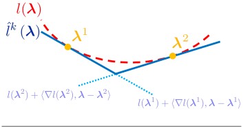
CPA recovers the optimal solution to RiskSlimMINLP by repeatedly solving a surrogate problem that optimizes a linear approximation of the loss function . The approximation is built using cutting planes or cuts. Each cut is a supporting hyperplane to the loss function at a fixed point :
Here, and are cut parameters that can be computed by evaluating the value and gradient of the loss at the point :
| (3) |
As shown in Figure 2, we can construct a cutting plane approximation of the loss function by taking the pointwise maximum of multiple cuts. In what follows, we denote the cutting plane approximation of the loss function built using cuts as:
On iteration , CPA solves a surrogate mixed-integer program (MIP) that minimizes the cutting plane approximation , namely . CPA uses the optimal solution to the surrogate MIP in two ways: (i) it computes a new cut at to improve the cutting plane approximation; (ii) it computes bounds on optimal value of RiskSlimMINLP to check for convergence. Here, the upper bound is set as the objective value of the best solution across all iterations:
| The lower bound is set as the optimal value of the surrogate problem at the current iteration: | ||||
CPA converges to an optimal solution of RiskSlimMINLP in a finite number of iterations (see e.g., Kelley, 1960, for a proof). In particular, the cutting plane approximation of a convex loss function improves monotonically with each cut:
Since the cuts added at each iteration are not redundant, the lower bound improves monotonically with each iteration. Once the optimality gap is less than a stopping threshold , CPA terminates and returns an -optimal solution to RiskSlimMINLP.
Key Benefits of Cutting Plane Algorithms
CPA has three important properties that motivate why we want to use a cutting plane algorithm to solve the risk score problem:
-
(i)
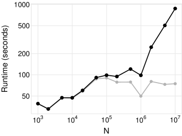
Scalability in the Sample Size: Cutting plane algorithms use the training data only when computing cut parameters, and not while solving RiskSlimMIP. Since the parameters in (3) can be computed using elementary matrix-vector operations in O() time at each iteration, running time scales linearly in for fixed (see Figure 3).
-
(ii)
Control over Data-related Computation: Cutting plane algorithms compute cut parameters in a single isolated step (e.g., Step 13 in Algorithm 1). Users can reduce data-related computation by customizing their implementation to compute these cut parameters efficiently (e.g., via distributed computing, or techniques that exploit structural properties of a specific model class as in Section E.2).
-
(iii)
Ability to use a MIP Solver: Cutting plane algorithms have a special benefit in our setting since the surrogate problem can be solved with a MIP solver (rather than a MINLP solver). MIP solvers provide a fast implementation of branch-and-bound search and other features to speed up the search process (e.g., built-in heuristics, preprocessing and cut generation procedures, lazy evaluation of cut constraints, and control callbacks that let us customize the search with specialized techniques). As we show in Figure 6, using a MIP solver can substantially improve our ability to solve RiskSlimMINLP, despite the fact that one may have to solve multiple MIPs.
Stalling in Non-Convex Settings
Cutting plane algorithms for empirical risk minimization (Joachims, 2006; Franc and Sonnenburg, 2008; Teo et al., 2009) are similar to CPA in that they solve a surrogate optimization problem at each iteration (e.g., Step 12 of Algorithm 1). When these algorithms are used to solve convex risk minimization problems, the surrogate is convex and therefore tractable. When the algorithms are used to solve risk minimization problems with non-convex regularizers or constraints, however, the surrogate is non-convex. In these settings, cutting plane algorithms will typically stall as they eventually reach an iteration where the surrogate problem cannot be solved to optimality within a fixed time limit.
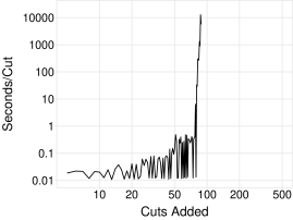
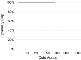
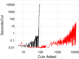
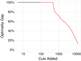
In Figure 4, we illustrate the stalling behavior of CPA on a difficult instance of RiskSlimMINLP for a synthetic dataset where (see also Figure 6). As shown, the first iterations terminate quickly as the surrogate problem RiskSlimMIP contains a trivial approximation of the loss. Since the surrogate becomes increasingly difficult to optimize with each iteration, however, the time to solve RiskSlimMIP increases exponentially, leading CPA to stall at iteration . In this case, the solution returned by CPA after 6 hours has a large optimality gap and a highly suboptimal loss. This is unsurprising, as the solution was obtained by optimizing a low-fidelity approximation of the loss (i.e., an 85-cut approximation of a 20-dimensional function). Since the value of the loss is tied to the performance of the model (see Section 5), the solution corresponds to a risk score with poor performance.
 |
 |
There is no simple fix to prevent standard cutting plane algorithms such as CPA from stalling on non-convex problems. This is because they need a globally optimal solution to a surrogate optimization problem at each iteration to compute a valid lower bound. In non-convex risk minimization problems, this requires finding the optimal solution of a non-convex surrogate problem, and certifying that there does not exist a better solution to the surrogate problem. If, for example, CPA only solved the surrogate until it found a feasible solution with a non-zero optimality gap, then it could produce a cutting plane that discards the true optimal solution. In this case, the lower bound computed in Step 15 would exceed the true optimal value, leading the algorithm to terminate prematurely and return a suboptimal solution with invalid bounds.
3.2 The Lattice Cutting Plane Algorithm
To avoid stalling in non-convex settings, we solve the risk score problem using the lattice cutting plane algorithm (LCPA) shown in Algorithm 2. LCPA has the same benefits as other cutting plane algorithms for the risk score problem, such as scalability in the sample size, control over data-related computation, and the ability to use a MIP solver. As shown in Figure 5, however, LCPA does not stall. This is because it can add cuts and compute a lower bound without having to optimize a non-convex surrogate.
 |
 |
LCPA recovers the optimal solution to RiskSlimMINLP via branch-and-bound (B&B) search. The search process recursively splits the feasible region of RiskSlimMINLP, discarding parts that are infeasible or provably suboptimal. LCPA solves a surrogate linear program (LP) over each region. It updates the cutting plane approximation when the surrogate LP yields an integer feasible solution. At that point, it sets the lower bound for the risk score problem as the smallest lower bound of the surrogate LP over unexplored regions.
Definition 2 (RiskSlimLP).
Given a bounded convex region , trade-off parameter , cutting plane approximation with cut parameters , and bounds , , , , , , the surrogate optimization problem can be formulated as the linear program:
| {equationarray}@crcl¿ l¿ r@ min_L,λ,α & V |
Branch-and-Bound Search
In Algorithm 2, we represent the state of the B&B search process using a B&B tree. We refer to each leaf of the tree as a node, and denote the set of all nodes as . Each node consists of: a region of the convex hull of the coefficient set ; and a lower bound on the objective value of the surrogate LP over this region . Each iteration of LCPA removes a node from the node set , then solves the surrogate LP for the corresponding region, that is, . Subsequent steps of the algorithm are determined by the solution status of the surrogate LP: If has an integer solution, LCPA updates the cutting plane approximation with a new cut at in Step 24. If has a real-valued solution, LCPA adds two child nodes and to the node set in Step 33. The child nodes are produced by applying a splitting rule, which splits into disjoint regions and . The lower bound for each child node is set as the optimal value of the surrogate LP . If is infeasible, then LCPA discards the node from the node set. The B&B search is governed by two procedures that are implemented in a MIP solver: RemoveNode, which removes a node ( from the node set (e.g., the node with the smallest lower bound ). SplitRegion, which splits into disjoint subsets of (e.g., split on a fractional component of , which returns and ). The output conditions for SplitRegion must ensure that the regions at each node remain disjoint, the total number of nodes remains finite, and the total search region shrinks even when the surrogate LP has a real-valued solution. LCPA evaluates the optimality of solutions to the risk score problem by using bounds on the objective value of RiskSlimMINLP. The upper bound is set as the objective value of the best integer feasible solution in Step 26. The lower bound is set as the smallest objective value among all nodes in Step 35. The value of can be viewed as a lower bound on the objective value of the surrogate LP over the remaining search region (i.e., is a lower bound on the objective value of ). Thus, will increase when we reduce the remaining search region or add cuts. Each iteration of LCPA reduces the remaining search region by either finding an integer feasible solution, identifying an infeasible region, or splitting a region into disjoint subsets. Thus, increases monotonically as the search region becomes smaller, and cuts are added at integer feasible solutions. Likewise, decreases monotonically as it is set as the objective value of the best integer feasible solution. Since there are a finite number of nodes, even in the worst-case, LCPA terminates after a finite number of iterations, returning an optimal solution to the risk score problem.Remark 3 (Worst-Case Data-Related Computation for LCPA).
Given any training dataset , any trade-off parameter , and any finite coefficient set , LCPA returns an optimal solution to the risk score problem after computing at most cutting planes, and processing at most nodes.Implementation with a MIP Solver with Lazy Cut Evaluation
LCPA can easily be implemented using a MIP solver (e.g., CPLEX, Gurobi, GLPK) with control callbacks. In this approach, the solver handles the B&B related steps of Algorithm 2, and one needs only to write a few lines of code to update the cutting plane approximation when the algorithm finds an integer feasible solution. In a basic implementation, the solver would call the control callback when it finds an integer feasible solution (i.e., Step 22). The code would retrieve the integer feasible solution, compute the cut parameters, and add a cut to the surrogate LP, handing control back to the solver at Step 25. A key benefit of using a MIP solver is the ability to add cuts as lazy constraints. In practice, if we were to add cuts as generic constraints to the surrogate LP, the time to solve the surrogate LP would increase with each cut, which would progressively slow down LCPA. When we add cuts as lazy constraints, the solver branches using a surrogate LP that contains a subset of relevant cuts, and only evaluates the complete set of cuts when LCPA finds an integer feasible solution. In this case, LCPA still returns the optimal solution. However, computation is significantly reduced as the surrogate LP is much faster to solve for the vast majority of cases where it is infeasible or yields a real-valued solution. From a design perspective, lazy cut evaluation reduces the marginal computational cost of adding cuts, which allows us to add cuts liberally (i.e., without having to worry about slowing down LCPA by adding too many cuts).3.3 Performance Comparison with MINLP Algorithms
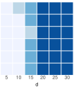
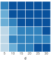
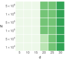
In what follows, we benchmark CPA and LCPA against three MINLP algorithms as implemented in a commercial MINLP solver (Artelsys Knitro 9.0, which is an updated version of the solver in Byrd et al., 2006). In Figure 6, we show the performance of algorithms on difficult instances of the risk score problem for synthetic datasets with dimensions and samples (see Appendix D for details). We consider the following performance metrics: (i) the time to find a near-optimal solution; (ii) the optimality gap of the best solution at termination; and (iii) the proportion of time spent on data-related computation. Since all three MINLP algorithms behave similarly, we only show the best one in Figure 6 (i.e., ActiveSetMINLP), and include results for the others in Appendix D.3. As shown, LCPA finds an optimal or near-optimal solution for almost all instances of the risk score problem, and pairs the solution with a small optimality gap. CPA performs similarly to LCPA on low-dimensional instances. On instances with , however, CPA stalls after a few iterations and returns a highly suboptimal solution (i.e., a risk score with poor performance). In comparison, the MINLP algorithms can only handle instances with small or . On larger instances, the solver is slowed down by operations that involve data-related computation, fails to converge within the 6-hour time limit and fails to recover a high-quality solution. Seeing how MINLP solvers are designed to solve a diverse set of optimization problems, we do not believe that they can identify and exploit the structure of the risk score problem in the same way as a cutting plane algorithm. LCPA CPA ActiveSetMINLP Time to Train a Good Risk Score i.e., the time for an algorithm to find a solution whose loss is of the optimal loss. This reflects the time to obtain a risk score with good calibration without a proof of optimality.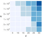
 Optimality Gap of Best Solution at Termination
i.e., , where is the objective value of the best solution found at termination. A gap of 0.0% means an algorithm has found the optimal solution and provided a proof of optimality within 6 hours.
Optimality Gap of Best Solution at Termination
i.e., , where is the objective value of the best solution found at termination. A gap of 0.0% means an algorithm has found the optimal solution and provided a proof of optimality within 6 hours.
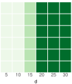
 % Time Spent on Data-Related Computation
i.e., the proportion of total runtime that an algorithm spends computing the value, gradient, or Hessian of the loss function.
% Time Spent on Data-Related Computation
i.e., the proportion of total runtime that an algorithm spends computing the value, gradient, or Hessian of the loss function.
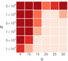
 Figure 6: Performance of LCPA, CPA, and a commercial MINLP solver on difficult instances of RiskSlimMINLP for synthetic datasets with dimensions and samples (see Appendix D for details).
ActiveSetMINLP fails to produce good risk scores on instances with large or as it struggles with data-related computation.
CPA and LCPA scale linearly in when is fixed: if they solve an instance for a given , then they can solve instances for larger in additional time. CPA stalls when and returns a low-quality risk score when . In contrast, LCPA consistently recovers a good model without stalling.
Results reflect the performance for a basic LCPA implementation without the improvements in Section 4. We show results for two other MINLP algorithms in Appendix D.
Figure 6: Performance of LCPA, CPA, and a commercial MINLP solver on difficult instances of RiskSlimMINLP for synthetic datasets with dimensions and samples (see Appendix D for details).
ActiveSetMINLP fails to produce good risk scores on instances with large or as it struggles with data-related computation.
CPA and LCPA scale linearly in when is fixed: if they solve an instance for a given , then they can solve instances for larger in additional time. CPA stalls when and returns a low-quality risk score when . In contrast, LCPA consistently recovers a good model without stalling.
Results reflect the performance for a basic LCPA implementation without the improvements in Section 4. We show results for two other MINLP algorithms in Appendix D.
4 Algorithmic Improvements
In this section, we describe specialized techniques to improve the performance of the lattice cutting plane algorithm (LCPA) on the risk score problem. They include: Polishing Heuristic. We present a technique called discrete coordinate descent (DCD; Section 4.1), which we use to polish integer solutions found by LCPA (solutions satisfying the condition in Step 22). DCD aims to improve the objective value of all integer solutions, which produces stronger upper bounds over the course of LCPA, and reduces the time to recover a good risk score. Rounding Heuristic. We present a rounding technique called SequentialRounding (Section 4.2) to generate integer solutions. We use SequentialRounding to round real-valued solutions of the surrogate LP (which are solutions that satisfy the condition in Step 31) and then polish the rounded solution with DCD. Rounded solutions may improve the best solution found by LCPA, producing stronger upper bounds and reducing the time to recover a good risk score. Bound Tightening Procedure. We design a fast procedure to strengthen bounds on the optimal values of the objective, loss, and number of non-zero coefficients called ChainedUpdates (Section 4.3). We call ChainedUpdates whenever the solver updates the upper bound in Step 26 or the lower bound in Step 35. ChainedUpdates improves the lower bound, and reduces the optimality gap of the final risk score. We present additional techniques to improve LCPA in Appendix E such as an initialization procedure and techniques to reduce data-related computation.4.1 Discrete Coordinate Descent
Discrete coordinate descent (DCD) is a technique to polish an integer solution (Algorithm 3). It takes as input an integer solution and iteratively changes a single coordinate to attain an integer solution with a better objective value. The coordinate at each iteration is set to minimize the objective value, i.e., . DCD terminates once it can no longer strictly improve the objective value along any coordinate. This eliminates the potential of cycling, and thereby guarantees that the procedure will terminate in a finite number of iterations. The polished solution returned by DCD satisfies a type of local optimality guarantee for discrete optimization problems. Formally, it is 1-opt with respect to the objective value, meaning that one cannot improve the objective value by changing any single coefficient (see e.g., Park and Boyd, 2018, for a technique to find a 1-opt point for a different optimization problem). In practice, the most expensive computation in DCD is finding a step-size that minimizes the objective along coordinate (Step 11 of Algorithm 3). We can significantly reduce this computation by using golden section search. This approach requires flops per iteration compared to flops per iteration required by a brute force approach (i.e., which evaluates the loss for all ). Algorithm 3 Discrete Coordinate Descent (DCD) 1: 2: training data 3: coefficient set 4: penalty parameter 5: integer solution to RiskSlimMINLP 6: valid descent directions 7:repeat 8: objective value at current solution 9: for do 10: list feasible moves along dim 11: find best move in dim 12: store objective value for best move in dim 13: end for 14: descend along dim that minimizes objective 15: 16:until 17: solution that is 1-opt with respect to the objective of RiskSlimMINLP In Figure 7, we show how DCD improves the performance of LCPA when we use it to polish feasible solutions found by the MIP solver (i.e., the polishing is placed just after Step 22 of Algorithm 2).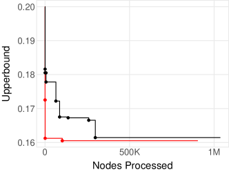
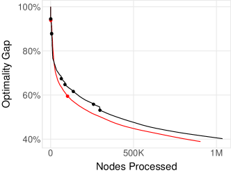 Figure 7: Performance profile of LCPA in a basic implementation (black) and with DCD (red). We use DCD to polish every integer solution found by the MIP solver whose objective value is within 10% of the current upper bound. We plot the number of total nodes processed of LCPA (x-axis) against the upper bound (y-axis; left) and the optimality gap (y-axis; right). We mark iterations where LCPA updates the incumbent solution. Results reflect performance on RiskSlimMINLP for a synthetic dataset with and 50,000 (see Appendix D for details).
4.2 Sequential Rounding
SequentialRounding (Algorithm 4) is a rounding heuristic to generate integer solutions for the risk score problem. In comparison to naïve rounding, which returns the closest rounding from a set of possible roundings, SequentialRounding returns a rounding that iteratively finds a local optimizer of the risk score problem. Given a real-valued solution , the procedure iteratively rounds one component (up or down) in a way that reduces the objective of RiskSlimMINLP. On iteration , it has already rounded components of , and must round one of the remaining components to or . To this end, it computes the objective of all feasible (component, direction)-pairs and chooses the best one. Formally, the minimization on iteration requires evaluations of the loss function. Thus, given that there are iterations, SequentialRounding terminates after evaluations of the loss function. In Figure 8, we show the impact of using SequentialRounding in LCPA. Here, we apply SequentialRounding to the non-integer solution of RiskSlimLP when the lower bound changes (i.e., just after Step 19 of Algorithm 2), then polish the rounded solution using DCD. As shown, this strategy can reduce the time required for LCPA to find a high-quality risk score, and attain a lower optimality gap. Algorithm 4 SequentialRounding 1: 2: training data 3: coefficient set 4: penalty parameter 5: non-integer infeasible solution from RiskSlimLP 6: index set of non-integer coefficients 7:repeat 8: for all 9: for all 10: 11: 12: if then 13: and 14: else 15: and 16: end if 17: 18:until 19: integer solution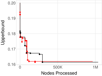
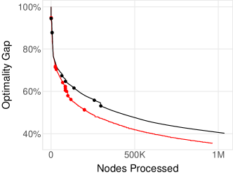 Figure 8: Performance profile of LCPA in a basic implementation (black) and with SequentialRounding and DCD polishing (red). We call SequentialRounding to round non-integer solutions to RiskSlimLP in Step 31, and then polish the integer solution with DCD. We plot large points to show when LCPA updates the incumbent solution. Results reflect performance on RiskSlimMINLP for a synthetic dataset with and 50,000 (see Appendix D for details). Here, SequentialRounding and DCD reduce the upper bound and optimality gap of LCPA compared to a basic implementation.
4.3 Chained Updates
We describe a fast bound tightening technique called ChainedUpdates (Algorithm 5). This technique iteratively bounds the optimal values of the objective, loss, and -norm by iteratively setting the values of , , , , and in RiskSlimLP. Bounding these quantities over the course of B&B restricts the search region without discarding the optimal solution, thereby improving the lower bound and reducing the optimality gap.Initial Bounds on Objective Terms
We initialize ChainedUpdates with values of , , , , and that can be computed using only the training data and the coefficient set . We start with Proposition 4, which provides initial values for and using the fact that the coefficient set is bounded.Proposition 4 (Bounds on Logistic Loss over a Bounded Coefficient Set)
Given a training dataset where and for , consider the normalized logistic loss of a linear classifier with coefficients : If the coefficients belong to a bounded set , then the value of the normalized logistic loss must obey where: The value of in Proposition 4 represents the “best-case” loss in a separable setting where we assign each positive example its maximal score , and each negative example its minimal score . Conversely, represents the “worst-case” loss when we assign each positive example its minimal score and each negative example its maximal score . We initialize the bounds on the number of non-zero coefficients to , trivially. In some cases, these bounds may be stronger due to operational constraints (e.g., we can set if models are required to use features). Having initialized , , and , we set the bounds on the optimal objective value as and , respectively.Dynamic Bounds on Objective Terms
In Propositions 5 to 7, we present bounds that can use information from the solver in LCPA to strengthen the values of , , , and (see Appendix A for proofs).Proposition 5 (Upper Bound on Optimal Number of Non-Zero Coefficients)
Given an upper bound on the optimal value , and a lower bound on the optimal loss , the optimal number of non-zero coefficients is at mostProposition 6 (Upper Bound on Optimal Loss)
Given an upper bound on the optimal value , and a lower bound on the optimal number of non-zero coefficients , the optimal loss is at mostProposition 7 (Lower Bound on Optimal Loss)
Given a lower bound on the optimal value , and an upper bound on the optimal number of non-zero coefficients , the optimal loss is at leastImplementation
In Algorithm 5, we present a bound-tightening procedure that uses the results of Propositions 5 to 7 to strengthen the values of , , , , and in RiskSlimLP. Algorithm 5 ChainedUpdates 1: 2: penalty parameter 3:, , , , , initial bounds on , and 4:repeat 5: update lower bound on 6: update upper bound on 7: update lower bound on 8: update upper bound on 9: update upper bound on 10:until there are no more bound updates due to Steps 5 to 9. 11:, , , , , Propositions 5 to 7 impose dependencies between , , , , and that may produce a complex “chain” of updates. As shown in Figure 9, ChainedUpdates can update multiple terms, and may update the same term more than once. Consider a case where we call ChainedUpdates after LCPA improves . Say the procedure updates in Step 7. If ChainedUpdates updates in Step 9, then it will also update , , , and . However, if ChainedUpdates does not update in Step 9, then it will not update , , , and terminate. Considering these dependencies, Algorithm 5 applies Propositions 5 to 7 until it can no longer improve , , , or . This ensures that ChainedUpdates will return its strongest possible bounds regardless of the term that was first updated.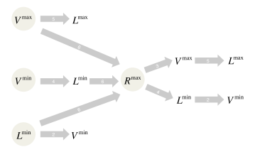 Figure 9: All possible “chains” of updates in ChainedUpdates. Circles represent “source” terms that can be updated by LCPA to trigger ChainedUpdates. The path from each source term shows all bounds that can be updated by the procedure. The number in each arrow references the update step in Algorithm 5.
In our implementation, we call ChainedUpdates whenever LCPA improves or (i.e., Step 26 or Step 35 of Algorithm 2). If ChainedUpdates improves any bounds, we pass this information back to the solver by updating the bounds on the auxiliary variables in the RiskSlimLP (Definition 2). As shown in Figure 10, this technique can considerably improve the lower bound and optimality gap over the course of LCPA.
Figure 9: All possible “chains” of updates in ChainedUpdates. Circles represent “source” terms that can be updated by LCPA to trigger ChainedUpdates. The path from each source term shows all bounds that can be updated by the procedure. The number in each arrow references the update step in Algorithm 5.
In our implementation, we call ChainedUpdates whenever LCPA improves or (i.e., Step 26 or Step 35 of Algorithm 2). If ChainedUpdates improves any bounds, we pass this information back to the solver by updating the bounds on the auxiliary variables in the RiskSlimLP (Definition 2). As shown in Figure 10, this technique can considerably improve the lower bound and optimality gap over the course of LCPA.
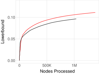
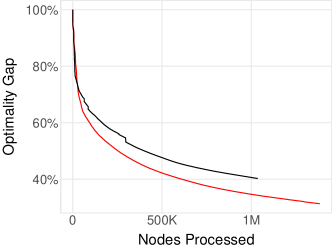 Figure 10: Performance profile of LCPA in a basic implementation (black) and with ChainedUpdates (red). Results reflect performance on a RiskSlimMINLP instance for a synthetic dataset with and 50,000 (see Appendix D).
5 Experiments
In this section, we compare the performance of methods to create risk scores. We have three goals: (i) to benchmark the performance and computation of our approach on real-world datasets; (ii) to highlight pitfalls of traditional approaches used in practice; and (iii) to present new approaches that address the pitfalls of traditional approaches.5.1 Setup
We considered 6 publicly available datasets shown in Table 2. We chose these datasets to see how methods are affected by factors such as class imbalance, the number of features, and feature encoding. For each dataset, we fit risk scores using RiskSLIM and 6 baseline methods that post-processed the coefficients of the best logistic regression model built using Lasso, Ridge or Elastic Net. We used each method to fit a risk score with small integer coefficients that obeys the model size constraint . We benchmarked each method for target model sizes Dataset Conditions for Reference income 32,561 36 24.1% person in 1994 US census earns over $50,000 Kohavi (1996) mammo 961 14 46.3% person has breast cancer Elter et al. (2007) mushroom 8,124 113 48.2% mushroom is poisonous Schlimmer (1987) rearrest 22,530 48 59.0% person is arrested after release from prison Zeng et al. (2017) spambase 4,601 57 39.4% e-mail is spam Cranor and LaMacchia (1998) telemarketing 41,188 57 11.3% person opens bank account after marketing call Moro et al. (2014) Table 2: Datasets used in Section 5. All datasets are available on the UCI repository (Bache and Lichman, 2013), other than rearrest which must be requested from ICPSR. We processed each dataset by dropping examples with missing values, and by binarizing categorical variables and some real-valued variables. We provide processed datasets and the code to process rearrest at http://github.com/ustunb/risk-slim.RiskSLIM
We formulated an instance of RiskSlimMINLP with the constraints: , , and . We set the trade-off parameter to a small value to recover the sparsest model among equally accurate models (see Appendix B). We solved each instance for at most 20 minutes on a 3.33 GHz CPU with 16 GB RAM using CPLEX 12.6.3 (ILOG, 2017).Penalized Logistic Regression
PLR is the best logistic regression model produced over the full regularization path using a weighted combination of the and penalties (i.e., the best model produced by Lasso, Ridge or Elastic Net). We train PLR models using the glmnet package of Friedman et al. (2010). The coefficients of each model are the solution to the optimization problem: where is the elastic-net mixing parameter and is a regularization penalty. We trained 1,100 PLR models by choosing 1,100 combinations of (): 11 values of 100 values of (chosen automatically by glmnet for each ). This free parameter grid produces 1,100 PLR models that include models obtained by: (i) Lasso (-penalty), which corresponds to PLR when ; (ii) Ridge (-penalty), which corresponds to PLR when ; (iii) standard logistic regression, which corresponds to PLR when and is small.Traditional Approaches
While there is considerable variation in how risk scores are developed in practice, many researchers follow a two-step approach: (i) fit a sparse logistic regression model with real-valued coefficients; (ii) convert it into a risk score with integer coefficients. We consider three methods that adopt this approach. Each method first trains a PLR model (i.e., the one that maximizes the 5-CV AUC and obeys the model size constraint), and then converts it into a risk score by applying a common rounding heuristic: PLRRd (Rounding): We round each coefficient to the nearest integer in by setting , and round the intercept as . PLRUnit (Unit Weighting): We round each coefficient to as . Unit weighting is a common heuristic in medicine and criminal justice (see e.g., Antman et al., 2000; Kessler et al., 2005; U.S. Department of Justice, 2005; Duwe and Kim, 2016), and sometimes called the Burgess method (as it was first proposed by Burgess, 1928). PLRRsRd (Rescaled Rounding) We first rescale coefficients so that the largest coefficient is , then round each coefficient to the nearest integer (i.e., where ). Rescaling is often used to avoid rounding small coefficients to zero, which happens when (see e.g., Le Gall et al., 1993).Pooled Approaches
We also propose three new methods that use a pooling strategy and the loss-minimizing heuristics from Section 4. Each method generates a pool of PLR models with real-valued coefficients, applies the same post-processing procedure to each model in the pool, then selects the best risk score among feasible risk scores. The methods include: PooledRd (Pooled PLR + Rounding): We fit a pool of 1,100 models using PLR. For each model in the pool, we round each coefficient to the nearest integer in by setting , and round the intercept as . PooledRd* (Pooled PLR + Rounding + Polishing): We fit a pool of 1,100 models using PooledRd. For each model in the pool, we polish the rounded coefficients using DCD. PooledSeqRd* (Pooled PLR + Sequential Rounding + Polishing): We fit a pool of 1,100 models using PLR. For each model in the pool, we round the coefficients using SequentialRounding and then polish the rounded coefficients using DCD. To ensure that the polishing step in PooledRd*and PooledSeqRd* does not increase the number of non-zero coefficients (which would violate the model size constraint), we run DCD only on the set (i.e., by fixing the set of zeros coefficients).Performance Evaluation
We evaluate the calibration of each risk score by plotting a reliability diagram, which shows how the predicted risk (x-axis) matches the observed risk (y-axis) for each distinct score (DeGroot and Fienberg, 1983). The observed risk at a score of is defined as If a model has over 30 distinct scores, we group them into 10 bins before plotting the reliability diagram. A model with perfect calibration should output predictions that are perfectly aligned with observed risk, as shown by a reliability diagram where all points lie on the line. We report the following summary statistics for each model: Calibration Error, computed as where is the predicted risk of example , and is the observed risk for all examples with a score of . CAL is the expected calibration error over the reliability diagram (see, e.g., Naeini et al., 2015). Area under the ROC curve, computed as where , . Note that trivial models (i.e., models that predict one class) achieve the best possible CAL (0.0%) but poor AUC (0.5). Logistic Loss, computed as . The loss reflects the objective values of the risk score problem when is small. We report the loss to see if minimizing the objective value of the risk score problem improves CAL and AUC. Model Size: the number of non-zero coefficients excluding the intercept .Parameter Tuning
We use nested 5-fold cross-validation (5-CV) to choose the free parameters of a final risk score (see Cawley and Talbot, 2010). The final risk score is fit using the entire dataset for an instance of the free parameters that satisfies the model size constraint and maximizes the 5-CV mean test AUC.5.2 Discussion
On the Performance of Risk Scores
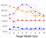
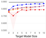
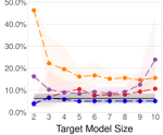
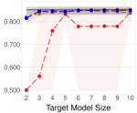
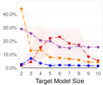
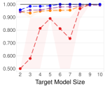
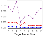
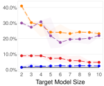
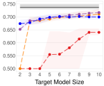
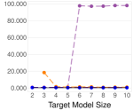
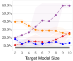
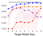
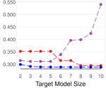
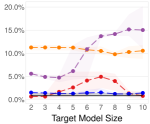
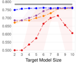
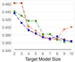
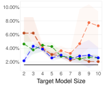
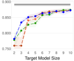
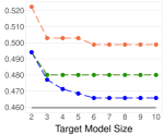
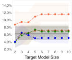
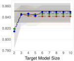
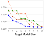
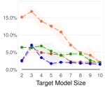
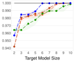
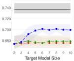
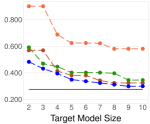
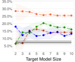
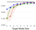
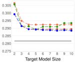
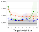
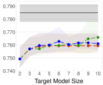
We compare the performance of RiskSLIM to traditional approaches in Figure 11, and to pooled approaches in Figure 12. These results show that RiskSLIM models consistently attain better calibration and AUC than alternatives. We present these results in greater detail for risk scores with a target model size of in Table 3. Here, RiskSLIM has the best 5-CV mean test CAL on 5/6 datasets, the best 5-CV mean test AUC on 5/6 datasets, and no method has better test CAL and test AUC than RiskSLIM.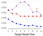
 mammo
mammo
 mushroom

 rearrest
 spambase
 telemarketing
 mammo
mammo
 mushroom
 rearrest
 spambase
 telemarketing
On the Caveats of CAL
The PLRRd risk score for telemarketing in Table 3 highlights a key shortcoming of CAL that illustrates why we report AUC: trivial and near-trivial models can have misleadingly low CAL. Here, PLRRd rounds all coefficients other than the intercept to zero, producing a model that trivially assigns a constant score to all examples . Since there is only one score, the predicted risk for all points is ,and the observed risk is the proportion of positive examples . Thus, a trivial model has a training CAL of 0.7%, the lowest among all methods, which (misleadingly) suggests that it has the best performance on training data (see Table LABEL:Table::GeneralizationResults in Appendix LABEL:Appendix::Experiments for values of training CAL). In this case, one could instead determine that the model is trivial by its training AUC, which is 0.500. This result also shows why we choose free parameters that maximize the 5-CV mean test AUC rather than CAL: choosing free parameters to minimize the 5-CV mean test CAL can result in a trivial model. Traditional Approaches Pooled Approaches PLRRd PLRRsRd PLRUnit PooledRd PooledRd* PooledSeqRd* RiskSLIM incomeOn Calibration Issues of Risk Scores
The reliability diagrams in Figure 13 highlight two issues with respect to the calibration of risk scores that are difficult to capture using a summary statistic: Monotonicity violations in observed risk. For example, the reliability diagrams for PLRRd on spambase, or PooledRd and PooledSeqRd* on mushroom show that the observed risk does not increase monotonically with predicted risk. There is not a way to calibrate the risk scores to remove this, and it is non-intuitive to have an increase in risk score correspond to a decrease in actual risk. Irregular spacing and coverage of predicted risk. For example, the PLRRd risk score for income outputs risk predictions that range between only 20% to 60%, and the PLRRsRd risk score for rearrest produces risk predictions that are clustered at end points. The results in Figure 13 suggest that such issues can be mitigated by optimizing the logistic loss (see, e.g., the calibration of risk scores built using RiskSLIM, PooledRd*, PooledSeqRd* where integer coefficients are determined by directly optimizing the logistic loss). In contrast, these issues are difficult to address by post-processing. Consider, for example, using Platt scaling (Platt, 1999) to improve the calibration of the PLRRd and PLRRsRd risk scores in Figure 13. As shown in Figure 14, Platt scaling improves calibration by centering and spreading risk estimates over the reliability diagram. However, it does not resolve issues that were introduced by earlier heuristics, such as monotonicity violations, a lack of coverage in risk predictions, or low AUC. Rounding Rescaled Rounding Raw + Platt Scaling Raw + Platt Scaling RiskSLIM incomeOn the Pitfalls of Traditional Approaches
Our results in Figure 11 and Table 3 show that risk scores built using traditional approaches perform poorly in terms of CAL and AUC. In particular: Rounding (PLRRd) produces risk scores with low AUC when it eliminates features from the model by rounding small coefficients to zero. Rescaled rounding (PLRRsRd) hurts calibration since the logistic loss is not scale-invariant (see e.g., the reliability diagram for rearrest PLRRsRd in Figure 13). Unit weighting (PLRUnit) results in poor calibration and unpredictable behavior (e.g., risk scores with more features can perform worse as seen in PLRUnit models for income and telemarketing in Figure 11). The effects of rescaled rounding and unit weighting on calibration are reflected by highly suboptimal values of the loss in Table 3 and Figure 11. These issues are often overlooked, perhaps because their effect on AUC is far less severe (e.g. the rescaling is recommended by U.S. Department of Justice, 2005; Pennsylvania Commission on Sentencing, 2012). Our baseline methods may not match the exact methods used in practice as they do not reflect the significant human input used in risk score development (e.g., domain experts perform preliminary feature selection, round coefficients, or choose a scaling factor before rounding, manually or without validation, as shown in Appendix C). Nevertheless, these results highlight two major pitfalls of traditional approaches, namely: Traditional approaches heuristically post-process a single model. This means that they fail whenever a heuristic dramatically changes CAL or AUC. Traditional approaches use heuristics that are oblivious to the value of the loss function, which tends to result in poor calibration.On Pooled Approaches
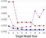
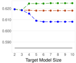
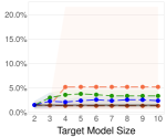
Our results suggest that risk scores built using our pooled approaches attain considerably better calibration and rank accuracy than those built using traditional approaches. These methods aim to overcome the pitfalls of traditional approaches using two strategies: Pooling, which generates a pool of PLR models, post-processes each model to produce a pool of risk scores, and selects the best risk score within the pool. Pooling provides some robustness against failure modes of heuristics that dramatically alter performance (e.g., for rounding, it is very unlikely that the coefficients of all models in the pool will be rounded to zero). The performance gain due to pooling can be seen by comparing the results for PLRRd to PooledRd in Table 3. Loss-Sensitive Heuristics, such as SequentialRounding and DCD, which produce a pool of risk scores that attain lower values of the loss, and thereby let us select a risk score with better CAL and AUC. The performance gain due to loss-sensitive heuristics can be seen by comparing the results for PooledRd to PooledRd* in Table 3. The fact that RiskSLIM risk scores have lower loss compared to pooled methods shows that direct optimization can efficiently find solutions that may not be found by exhaustive post-processing (e.g., where we fit all possible and penalized logistic regression models, and convert them to risk scores with specially-designed heuristics). Here, we have shown that exhaustive post-processing strategies can often produce risk scores that perform well. In Section 6, however, we will see that the performance gap can be significant in the presence of non-trivial constraints.On Computation
Although the risk score problem is NP-hard, we trained RiskSLIM models that were certifiably optimal or had small optimality gaps for all datasets in under 20 minutes using an LCPA implementation with the improvements in Section 4. Even when LCPA did not recover a certifiably optimal solution, it produced a risk score that performed well and did not exhibit the calibration issues of models built heuristically. In general, the time spent computing cutting planes is a small portion of the overall runtime for LCPA (, for all datasets). Given that LCPA scales linearly with sample size, we expect to obtain similar results even if the datasets had far more samples. Factors that affected the time to obtain a certifiably optimal solution include: Highly Correlated Features: Subsets of redundant features produce multiple optima, which increases the size of the B&B tree. Feature Encoding: In particular, the problem is harder when the dataset includes real-valued variables, like those in the spambase dataset. Difficulty of the Learning Problem: On separable problems such as mushroom, it is easy to recover a certifiably optimal solution since many solutions perform well and produce a near-optimal lower bound.6 ICU Seizure Prediction
In this section, we describe a collaboration with the Massachusetts General Hospital and the University of Wisconsin Hospital where we built a customized risk score for ICU seizure prediction (Struck et al., 2017). Our goal is to discuss practical aspects of our approach on a real-world problem with non-trivial constraints.6.1 Problem Description
Patients who suffer from traumatic brain injury (e.g., due to a ruptured brain aneurysm) often experience seizures while they are in intensive care. Since seizures are not outwardly visible in this setting, but may lead to irreversible brain damage, patients who are brought into the ICU are monitored via continuous electroencephalography (cEEG). Based on current clinical standards, neurologists undergo extensive training to recognize a large set of patterns in cEEG output (see e.g., Figure 21 and Hirsch et al., 2013). They consider the presence and characteristics of cEEG patterns along with other medical information to evaluate a patient’s risk of seizure. These risk estimates are used to decide if a patient can be dismissed from the ICU, kept for further monitoring, or prescribed a medical intervention to avert potential brain injury. In practice, hospitals have a limited number of cEEG monitors that may be poorly assigned between patients in the ICU. Given reliable estimates of seizure risk, patients with a low risk of seizure can be taken off monitoring to free up monitors for new patients.
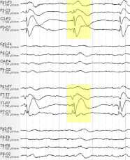 Figure 21: cEEG displays electrical activity at 16 standardized locations in a patient’s brain using electrodes placed on the scalp. We show two cEEG patterns: a Generalized Periodic Discharge (GPD), which occurs on both sides of the brain (left); and a Lateralized Periodic Discharge (LPD), which occurs on one side of the brain (right). These figures were reproduced from a presentation at a training module by the American Clinical Neurophysiology Society (2012).
Data
Our dataset was derived from cEEG recordings from 41 hospitals, curated by the Critical Care EEG Monitoring Research Consortium. It contains recordings and input variables (see Appendix LABEL:Appendix::SeizurePrediction for a list). The outcome is defined as if patient who has been in the ICU for the past 24 hours will have a seizure in the next 24 hours. There is significant class imbalance as = 12.5%. The input variables include information on patient medical history, secondary neurological symptoms, and the presence and characteristics of 5 standard cEEG patterns: Lateralized Periodic Discharges (LPD); Lateralized Rhythmic Delta (LRDA); Generalized Periodic Discharges (GPD); Generalized Rhythmic Delta (GRDA); and Bilateral Periodic Discharges (BiPD).Model Requirements
Our collaborators wanted a risk score to help them reliably predict seizure risk by checking the presence and characteristics of cEEG patterns. It was critical for the model to output calibrated risk predictions since physicians would use the predicted risk to choose between multiple treatment options (i.e., patients may be prescribed different medication based on their predicted risk; see also Van Calster and Vickers, 2015; Shah et al., 2018, for a discussion on how miscalibrated risk predictions can lead to harmful decisions). To be adopted by physicians, it was also important to build a model that could be validated by domain experts and that was aligned with domain expertise. In Figure 22, we present a RiskSLIM risk score for this problem that satisfies all of these requirements (see Struck et al., 2017, for details on model development). This risk score outputs calibrated risk estimates at several operating points. It obeys a model size constraint () to let physicians easily validate the model, and monotonicity constraints to ensure that the signs of some coefficients are aligned with domain knowledge.Training Setup
We used the training setup in Section 5.1, which we adapted to address constraints as follows. We trained a RiskSLIM model by solving a customized instance of RiskSlimMINLP with 20 additional constraints and 2 additional variables, which we solved to optimality in minutes. The baseline methods had built-in mechanisms to handle monotonicity constraints, but required tuning to handle other constraints. For each method, we trained a final model using all of the training data for the instance of the free parameters that obeyed all constraints and maximized the mean 5-CV test AUC.6.2 Discussion
Method Constraints Violated Test CAL Test AUC Model Size Loss Value Optimality Gap Train CAL Train AUC RiskSLIM – 2.5 1.9 - 3.4 0.801 0.758 - 0.841 4 4 - 4 0.293 0.0 2.0 0.806 PooledRd – 5.3 3.1 - 7.1 0.740 0.712 - 0.757 2 1 - 3 0.350 – 6.0 0.752 PooledRd* – 3.0 1.4 - 3.6 0.745 0.712 - 0.776 2 1 - 3 0.308 – 1.9 0.754 PooledSeqRd* – 2.8 2.4 - 3.1 0.745 0.713 - 0.805 3 2 - 4 0.313 – 1.9 0.767 PLR All 2.6 1.7 - 3.6 0.844 0.829 - 0.869 29 20 - 35 0.272 – 2.0 0.850 PLR Integrality Operational 4.4 3.3 - 6.5 0.742 0.712 - 0.774 4 3 - 4 0.325 – 3.9 0.771 PLRRd Operational 7.0 5.7 - 9.2 0.743 0.705 - 0.786 2 2 - 3 0.329 – 7.0 0.735 PLRRsRd Operational 12.4 11.2 - 13.6 0.761 0.733 - 0.815 4 4 - 4 2.109 – 12.5 0.760 PLRUnit Operational 24.6 23.6 - 25.7 0.759 0.732 - 0.813 4 4 - 4 0.520 – 24.8 0.759 Table 4: Performance of risk scores for seizure prediction, and feasibility with respect to constraints. We report the 5-CV mean test CAL and 5-CV mean test AUC. The ranges in each cell represent the 5-CV minimum and maximum. We present the risk scores built using each method in Figures 23 to 26.On Performance and Usability in a Constrained Setting
The results in Table 4 show the potential performance benefits of training an optimized risk score for problems with non-trivial constraints. Here, RiskSLIM has a 5-CV mean test CAL/AUC of 2.5%/0.801 while the best risk score built using a heuristic method has a 5-CV mean test CAL/AUC of 2.8%/0.745 In contrast to the experiments in Section 5, only RiskSLIM and our pooled methods were able to find a feasible risk score under the constraints. Traditional methods (e.g., PLRRd, PLRRsRd, and PLRUnit) violate one or more constraints after rounding. In fact, these methods cannot produce a risk score with comparable performance to the RiskSLIM risk score even when these constraints are relaxed. If we consider only simple constraints on model size and monotonicity, then risk scores produced by these methods have a test AUC of at most 0.761 (PLRRsRd) and a test CAL of at least 7.0% (PLRRd). As shown in Figures 23 to 26, risk scores with similar test CAL can still exhibit important differences in terms of calibration. Here, the risk predictions of the RiskSLIM model are monotonic and within the boundaries of the risk predictions of the fold-based models. In comparison, the risk predictions of other models do not monotonically increase with observed risk and vary significantly across test folds (e.g., PooledSeqRd*). As noted by our collaborators, such issues affect model adoption: the monotonicity violations of the PooledSeqRd model suggest that patients with a score of 3.5 may have more seizures compared to patients with a score of 4.0, eroding trust in the model’s risk predictions. Although the risk scores in Figures 23 to 26 obey all of the constraints specified by our collaborators, they exhibit differences in terms of usability. The RiskSLIM model requires physicians to check cEEG output for a single cEEG pattern (LPD). In comparison, other risk scores include the feature PatternsInclude BiPD or LRDA or LPD, which can require physicians to check cEEG output for 3 patterns in the worst case. The PooledSeqRd* risk score also uses MaxFrequencyLPD, which requires estimating the frequency of LPD and thereby requires more time.On the Value of the Optimality Gap in Practice
The results in Table 4 illustrate how heuristics may lead practitioners to overestimate the true impact of real-world constraints on model performance. Here: three traditional methods could not output a feasible risk score; six pooled methods produced feasible risk scores with suboptimal AUC and calibration issues; and a baseline PLR model with real-valued coefficients has an AUC of 0.742. Based on these results, a practitioner might inadvertently conclude that no feasible risk score could achieve a test AUC of 0.801. In contrast, RiskSLIM models are paired with an optimality gap. In practice, a small optimality gap suggests that we have trained the best possible risk score that satisfies a specific set of constraints. Thus, if a risk score with a small optimality gap performs poorly on training data, and the model generalizes (e.g., its training performance is similar to its K-CV performance), then one can attribute the performance deficit of the model to overly restrictive constraints and improve performance by relaxing them. This provides a general mechanism to evaluate the effect of constraints on performance. If, for example, that our collaborators were not satisfied with the performance or usability of our model, then we could train certifiably optimal risk scores for different sets of constraints. By comparing the performance of certifiably optimal models, our collaborators could evaluate the true impact of their requirements on predictive performance, and navigate trade-offs in an informed manner. This approach helped our collaborators decide between a model with 4 features or 5 features. Here, we trained a RiskSLIM risk score with 5 features, which has a 5-CV test CAL/AUC of 3.4%/0.816. However, the slight improvement in test AUC did not outweigh the fact that the larger model included the feature MaxFreqFactorAnyPattern which could increase the model evaluation time by doctors.On the Challenges of Handling Operational Constraints
One of the practical benefits of our approach is that it can address constraints without parameter tuning or post-processing. Since our approach can directly incorporate constraints into the MINLP formulation, all RiskSLIM models are feasible. Thus we can produce a feasible risk score and estimate its predictive performance by training 6 models: 1 final model fit on the full dataset for deployment, and 5 models trained on subsets of the training data to produce an unbiased performance estimate for the algorithm via 5-fold CV. In contrast, the pooled methods produce a feasible model by post-processing a large pool of models and discarding those that are infeasible. Since we must then choose between feasible models on the basis of 5-CV performance, we must use a nested CV setup to pair any model with an unbiased performance estimate. This requires fitting a total of 33,000 models.222A nested CV setup with 5 outer folds, 5 inner folds, and 1,100 free parameter instances requires fitting models. In general settings, there is no guarantee that pooled methods will produce a feasible risk score. In this case, for instance, only 12% of the instances for the pooled methods satisfied all constraints (see Table LABEL:Table::DemoFeasibilityTable in Appendix LABEL:Appendix::SeizurePrediction). This kind of massive testing can become computationally burdensome. Our results highlight other issues with methods that aim to address constraints by parameter tuning. Let us say we would use a standard -fold CV setup to tune parameters. In this case, we would train models on validation folds for each instance of the free parameters, choose the instance of the free parameters that maximizes the mean -CV test AUC without violating any constraints, and then train a “final model” for this instance. Unfortunately, there is no guarantee that the final model will obey all constraints.On the Benefits of Risk Scores with Small Integer Coefficients
Figures 23 to 26 illustrate some of the practical benefits of risk scores with small integer coefficients. When input variables belong to a small discrete set, the scores also belong to a small discrete set. This reduces the number of operating points on the ROC curve and reliability diagram, which makes it easier to pick an operating point. Further, when input variables are binary, the decision rules at each operating point can be represented as a Boolean rule. For the RiskSLIM model in Figure 23, for example, the decision rule: is equivalent to the Boolean function: BriefRhythmicDischarge Small integer coefficients let users extract such rules by listing conditions when the score exceeds the threshold. This is more challenging when a model uses real-valued coefficients, as shown by the score function of the PLR model from Table 4: In this case, extracting a Boolean function is difficult as computing the score involves arithmetic with real-valued coefficients and the real-valued variable MaxFrequencyLPD.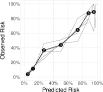
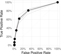
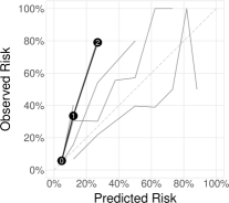
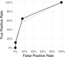
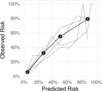
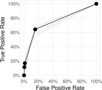
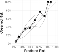
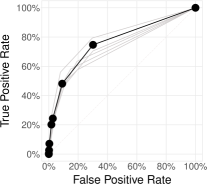
7 Concluding Remarks
Risk scores are simple tools that are often used to inform consequential decisions, such as mortality prediction and loan approval. Despite the fact that risk scores have been used in such tasks for nearly a century, they are often developed using ad hoc methods – i.e., by combining machine learning methods with heuristics (see e.g., the pipeline for the TIMI risk score in Antman et al., 2000, in Appendix C). In practice, such approaches may produce a risk score that violates important requirements, leading practitioners to make manual adjustments, or to build models without data (e.g., via a panel of domain experts as in Gage et al., 2001; McGinley and Pearse, 2012). Such approaches do not produce risk scores with performance guarantees, and may result in the deployment of models with poor calibration or rank accuracy. Ad hoc model development also has hidden costs. For example, the need to implement a specialized training pipeline slows down model development. Our goal in this paper was to design a machine learning approach to build risk scores that standardizes model development, reduces the need for domain experts to manually specify and tune models, and pairs models with useful guarantees. Our approach trains risk scores by solving an empirical risk minimization problem that performs exact feature selection while restricting coefficients to small integers and enforcing application-specific constraints. Since commercial solvers did not handle this problem well, we solved it with a new cutting plane algorithm (LCPA), which allows training to scale linearly with the number of samples, and can be used to solve other empirical risk minimization problems with non-convex regularizers or constraints. As shown in Sections 5 and 6, LCPA can train certifiably optimal risk scores for real-world datasets in minutes. These models often attain best-in-class calibration and rank accuracy, and avoid pitfalls of heuristics used in practice. Our approach simplifies model development, by letting practitioners customize risk scores without post-processing. In addition, it pairs models with a certificate of optimality, which can be used to understand how application-specific constraints affect predictive performance.Acknowledgments
We gratefully acknowledge support from Siemens, Phillips, and Wistron. We would like to thank Paul Rubin for helpful discussions, and our collaborators Aaron Struck and Brandon Westover for their guidance on the seizure prediction application.References
- Alba et al. [2017] Alba, Ana Carolina, Thomas Agoritsas, Michael Walsh, Steven Hanna, Alfonso Iorio, PJ Devereaux, Thomas McGinn, and Gordon Guyatt. Discrimination and calibration of clinical prediction models: Users’ guides to the medical literature. Journal of the American Medical Association, 318(14):1377–1384, 2017.
- American Clinical Neurophysiology Society [2012] American Clinical Neurophysiology Society. Standardized Critical Care EEG Terminology Training Module, 2012.
- Amodei et al. [2016] Amodei, Dario, Chris Olah, Jacob Steinhardt, Paul Christiano, John Schulman, and Dan Mané. Concrete problems in AI safety. arXiv preprint arXiv:1606.06565, 2016.
- Angelino et al. [2018] Angelino, Elaine, Nicholas Larus-Stone, Daniel Alabi, Margo Seltzer, and Cynthia Rudin. Learning certifiably optimal rule lists for categorical data. Journal of Machine Learning Research, 18(234):1–78, 2018.
- Antman et al. [2000] Antman, Elliott M, Marc Cohen, Peter JLM Bernink, Carolyn H McCabe, Thomas Horacek, Gary Papuchis, Branco Mautner, Ramon Corbalan, David Radley, and Eugene Braunwald. The TIMI risk score for unstable angina/non–ST elevation MI. Journal of the American Medical Association, 284(7):835–842, 2000.
- Austin et al. [2010] Austin, James, Roger Ocker, and Avi Bhati. Kentucky Pretrial Risk Assessment Instrument Validation. Bureau of Justice Statistics, 2010.
- Bache and Lichman [2013] Bache, K. and M. Lichman. UCI Machine Learning Repository, 2013.
- Bai and Rubin [2009] Bai, Lihui and Paul A Rubin. Combinatorial Benders Cuts for the Minimum Tollbooth Problem. Operations Research, 57(6):1510–1522, 2009.
- Bardenet and Maillard [2015] Bardenet, Rémi and Odalric-Ambrym Maillard. Concentration inequalities for sampling without replacement. Bernoulli, 21(3):1361–1385, 2015.
- Beneish et al. [2013] Beneish, Messod D, Charles MC Lee, and D Craig Nichols. Earnings manipulation and expected returns. Financial Analysts Journal, 69(2):57–82, 2013.
- Bertsimas et al. [2016] Bertsimas, Dimitris, Angela King, and Rahul Mazumder. Best subset selection via a modern optimization lens. The Annals of Statistics, 44(2):813–852, 2016.
- Billiet et al. [2017] Billiet, Lieven, Sabine Van Huffel, and Vanya Van Belle. Interval coded scoring extensions for larger problems. In Proceedings of the IEEE Symposium on Computers and Communications, pages 198–203. IEEE, 2017.
- Billiet et al. [2018] Billiet, Lieven, Sabine Van Huffel, and Vanya Van Belle. Interval Coded Scoring: A toolbox for interpretable scoring systems. PeerJ Computer Science, 4:e150, 04 2018.
- Bobko et al. [2007] Bobko, Philip, Philip L Roth, and Maury A Buster. The usefulness of unit weights in creating composite scores. A literature review, application to content validity, and meta-analysis. Organizational Research Methods, 10(4):689–709, 2007.
- Bonami et al. [2012] Bonami, Pierre, Mustafa Kilinç, and Jeff Linderoth. Algorithms and software for convex mixed integer nonlinear programs. In Mixed Integer Nonlinear Programming, pages 1–39. Springer, 2012.
- Boyd and Vandenberghe [2004] Boyd, Stephen P and Lieven Vandenberghe. Convex Optimization. Cambridge University Press, 2004.
- Burgess [1928] Burgess, Ernest W. Factors determining success or failure on parole. The workings of the indeterminate sentence law and the parole system in Illinois, pages 221–234, 1928.
- Byrd et al. [2006] Byrd, Richard H, Jorge Nocedal, and Richard A Waltz. KNITRO: An Integrated Package for Nonlinear Optimization. In Large-scale Nonlinear Optimization, pages 35–59. Springer, 2006.
- Calmon et al. [2017] Calmon, Flavio, Dennis Wei, Bhanukiran Vinzamuri, Karthikeyan Natesan Ramamurthy, and Kush R Varshney. Optimized pre-processing for discrimination prevention. In Advances in Neural Information Processing Systems, pages 3995–4004, 2017.
- Carrizosa et al. [2016] Carrizosa, Emilio, Amaya Nogales-Gómez, and Dolores Romero Morales. Strongly agree or strongly disagree?: Rating features in support vector machines. Information Sciences, 329:256–273, 2016.
- Caruana and Niculescu-Mizil [2004] Caruana, Rich and Alexandru Niculescu-Mizil. Data mining in metric space: an empirical analysis of supervised learning performance criteria. In Proceedings of the 10th ACM SIGKDD International Conference on Knowledge Discovery and Data Mining, pages 69–78. ACM, 2004.
- Caruana and Niculescu-Mizil [2006] Caruana, Rich and Alexandru Niculescu-Mizil. An empirical comparison of supervised learning algorithms. In Proceedings of the 23rd international conference on Machine Learning, pages 161–168. ACM, 2006.
- Caruana et al. [2015] Caruana, Rich, Yin Lou, Johannes Gehrke, Paul Koch, Marc Sturm, and Noemie Elhadad. Intelligible models for healthcare: Predicting pneumonia risk and hospital 30-day readmission. In Proceedings of the 21th ACM SIGKDD International Conference on Knowledge Discovery and Data Mining, pages 1721–1730. ACM, 2015.
- Cawley and Talbot [2010] Cawley, Gavin C and Nicola LC Talbot. On over-fitting in model selection and subsequent selection bias in performance evaluation. Journal of Machine Learning Research, 11(Jul):2079–2107, 2010.
- Chang et al. [2012] Chang, Allison, Cynthia Rudin, Michael Cavaretta, Robert Thomas, and Gloria Chou. How to reverse-engineer quality rankings. Machine Learning, 88:369–398, September 2012.
- Chen and Rudin [2018] Chen, Chaofan and Cynthia Rudin. An optimization approach to learning falling rule lists. In Proceedings of the 21st International Conference on Artificial Intelligence and Statistics, volume 84 of Proceedings of Machine Learning Research, pages 604–612. PMLR, 09–11 Apr 2018.
- Chen et al. [2018] Chen, Chaofan, Kancheng Lin, Cynthia Rudin, Yaron Shaposhnik, Sijia Wang, and Tong Wang. An interpretable model with globally consistent explanations for credit risk. In Proceedings of NeurIPS 2018 Workshop on Challenges and Opportunities for AI in Financial Services: the Impact of Fairness, Explainability, Accuracy, and Privacy, 2018.
- Chevaleyre et al. [2013] Chevaleyre, Yann, Frederic Koriche, and Jean-Daniel Zucker. Rounding methods for discrete linear classification. In Proceedings of the 30th International Conference on Machine Learning, pages 651–659, 2013.
- Cranor and LaMacchia [1998] Cranor, Lorrie Faith and Brian A LaMacchia. Spam! Communications of the ACM, 41(8):74–83, 1998.
- Dawes [1979] Dawes, Robyn M. The robust beauty of improper linear models in decision making. American Psychologist, 34(7):571–582, 1979.
- DeGroot and Fienberg [1983] DeGroot, Morris H and Stephen E Fienberg. The comparison and evaluation of forecasters. The Statistician, pages 12–22, 1983.
- Duwe and Kim [2016] Duwe, Grant and KiDeuk Kim. Sacrificing accuracy for transparency in recidivism risk assessment: The impact of classification method on predictive performance. Corrections, pages 1–22, 2016.
- Einhorn and Hogarth [1975] Einhorn, Hillel J and Robin M Hogarth. Unit weighting schemes for decision making. Organizational Behavior and Human Performance, 13(2):171–192, 1975.
- Elter et al. [2007] Elter, M, R Schulz-Wendtland, and T Wittenberg. The prediction of breast cancer biopsy outcomes using two CAD approaches that both emphasize an intelligible decision process. Medical Physics, 34:4164, 2007.
- Ertekin and Rudin [2011] Ertekin, Şeyda and Cynthia Rudin. On equivalence relationships between classification and ranking algorithms. Journal of Machine Learning Research, 12:2905–2929, 2011.
- Ertekin and Rudin [2015] Ertekin, Şeyda and Cynthia Rudin. A Bayesian Approach to Learning Scoring Systems. Big Data, 3(4):267–276, 2015.
- Feldman et al. [2015] Feldman, Michael, Sorelle A Friedler, John Moeller, Carlos Scheidegger, and Suresh Venkatasubramanian. Certifying and removing disparate impact. In Proceedings of the 21th ACM SIGKDD International Conference on Knowledge Discovery and Data Mining, pages 259–268. ACM, 2015.
- FICO [2011] FICO. Introduction to Scorecard for FICO Model Builder. http://www.fico.com/en/node/8140?file=7900, 2011.
- Finlay [2012] Finlay, Steven. Credit scoring, response modeling, and insurance rating: a practical guide to forecasting consumer behavior. Palgrave Macmillan, 2012.
- Franc and Sonnenburg [2008] Franc, Vojtěch and Soeren Sonnenburg. Optimized cutting plane algorithm for support vector machines. In Proceedings of the 25th International Conference on Machine Learning, pages 320–327. ACM, 2008.
- Franc and Sonnenburg [2009] Franc, Vojtěch and Sören Sonnenburg. Optimized cutting plane algorithm for large-scale risk minimization. Journal of Machine Learning Research, 10:2157–2192, 2009.
- Friedman et al. [2010] Friedman, Jerome, Trevor Hastie, and Robert Tibshirani. Regularization paths for generalized linear models via coordinate descent. Journal of Statistical Software, 33(1):1–22, 2010.
- Gage et al. [2001] Gage, Brian F, Amy D Waterman, William Shannon, Michael Boechler, Michael W Rich, and Martha J Radford. Validation of clinical classification schemes for predicting stroke. Journal of the American Medical Association, 285(22):2864–2870, 2001.
- Goel et al. [2016] Goel, Sharad, Justin M Rao, and Ravi Shroff. Precinct or Prejudice? Understanding Racial Disparities in New York City’s Stop-and-Frisk Policy. Annals of Applied Statistics, 10(1):365–394, 2016.
- Goh et al. [2016] Goh, Gabriel, Andrew Cotter, Maya Gupta, and Michael P Friedlander. Satisfying real-world goals with dataset constraints. In Advances in Neural Information Processing Systems, pages 2415–2423, 2016.
- Goh and Rudin [2014] Goh, Siong Thye and Cynthia Rudin. Box drawings for learning with imbalanced data. In Proceedings of the 20th ACM SIGKDD International Conference on Knowledge Discovery and Data Mining, pages 333–342. ACM, 2014.
- Goldberg and Eckstein [2012] Goldberg, Noam and Jonathan Eckstein. Sparse weighted voting classifier selection and its linear programming relaxations. Information Processing Letters, 112:481–486, 2012.
- Gottfredson and Snyder [2005] Gottfredson, Don M and Howard N Snyder. The mathematics of risk classification: Changing data into valid instruments for juvenile courts. NCJ 209158. Office of Juvenile Justice and Delinquency Prevention Washington, D.C., 2005.
- Guan et al. [2009] Guan, Wei, Alex Gray, and Sven Leyffer. Mixed-integer support vector machine. In NIPS Workshop on Optimization for Machine Learning, 2009.
- Gupta et al. [2016] Gupta, Maya, Andrew Cotter, Jan Pfeifer, Konstantin Voevodski, Kevin Canini, Alexander Mangylov, Wojciech Moczydlowski, and Alexander Van Esbroeck. Monotonic calibrated interpolated look-up tables. Journal of Machine Learning Research, 17(1):3790–3836, 2016.
- Hirsch et al. [2013] Hirsch, LJ, SM LaRoche, N Gaspard, E Gerard, A Svoronos, ST Herman, R Mani, H Arif, N Jette, Y Minazad, et al. American clinical neurophysiology society’s standardized critical care EEG terminology: 2012 version. Journal of Clinical Neurophysiology, 30(1):1–27, 2013.
- Holte [1993] Holte, Robert C. Very simple classification rules perform well on most commonly used datasets. Machine Learning, 11(1):63–90, 1993.
- Holte [2006] Holte, Robert C. Elaboration on Two Points Raised in “Classifier Technology and the Illusion of Progress”. Statistical Science, 21(1):24–26, February 2006.
- Hu et al. [2019] Hu, Xiyang, Cynthia Rudin, and Margo Seltzer. Optimal sparse decision trees. In Proc. Neural Information Processing Systems, 2019.
- ILOG [2017] ILOG, IBM. CPLEX Optimizer 12.6. https://www-01.ibm.com/software/commerce/optimization/cplex-optimizer/, 2017.
- Joachims [2006] Joachims, Thorsten. Training linear SVMs in linear time. In Proceedings of the 12th ACM SIGKDD International conference on Knowledge Discovery and Data Mining, pages 217–226. ACM, 2006.
- Joachims et al. [2009] Joachims, Thorsten, Thomas Finley, and Chun-Nam John Yu. Cutting-plane training of structural SVMs. Machine Learning, 77(1):27–59, 2009.
- Kamishima et al. [2011] Kamishima, Toshihiro, Shotaro Akaho, and Jun Sakuma. Fairness-aware learning through regularization approach. In 2011 IEEE 11th International Conference on Data Mining Workshops, pages 643–650. IEEE, 2011.
- Kelley [1960] Kelley, James E, Jr. The cutting-plane method for solving convex programs. Journal of the Society for Industrial and Applied Mathematics, 8(4):703–712, 1960.
- Kessler et al. [2005] Kessler, Ronald C, Lenard Adler, Minnie Ames, Olga Demler, Steve Faraone, EVA Hiripi, Mary J Howes, Robert Jin, Kristina Secnik, Thomas Spencer, et al. The World Health Organization Adult ADHD Self-Report Scale (ASRS): a short screening scale for use in the general population. Psychological Medicine, 35(02):245–256, 2005.
- Kohavi [1996] Kohavi, Ron. Scaling up the accuracy of naive-bayes classifiers: a decision-tree hybrid. In Proceedings of the Second International Conference on Knowledge Discovery and Data Mining, pages 202–207. AAAI Press, 1996.
- Kotlowski et al. [2011] Kotlowski, Wojciech, Krzysztof J Dembczynski, and Eyke Huellermeier. Bipartite ranking through minimization of univariate loss. In Proceedings of the 28th International Conference on Machine Learning, pages 1113–1120, 2011.
- Kronqvist et al. [2019] Kronqvist, Jan, David E Bernal, Andreas Lundell, and Ignacio E Grossmann. A review and comparison of solvers for convex MINLP. Optimization and Engineering, 20(2):397–455, 2019.
- Lakkaraju et al. [2016] Lakkaraju, Himabindu, Stephen H Bach, and Jure Leskovec. Interpretable decision sets: A joint framework for description and prediction. In Proceedings of the 22nd ACM SIGKDD International Conference on Knowledge Discovery and Data Mining, pages 1675–1684. ACM, 2016.
- Latessa et al. [2009] Latessa, Edward, Paula Smith, Richard Lemke, Matthew Makarios, and Christopher Lowenkamp. Creation and validation of the Ohio risk assessment system: Final report, 2009.
- Le Gall et al. [1993] Le Gall, Jean-Roger, Stanley Lemeshow, and Fabienne Saulnier. A new simplified acute physiology score (SAPS II) based on a European/North American multicenter study. Journal of the American Medical Association, 270(24):2957–2963, 1993.
- Letham et al. [2015] Letham, Benjamin, Cynthia Rudin, Tyler H. McCormick, and David Madigan. Interpretable classifiers using rules and Bayesian analysis: Building a better stroke prediction model. Annals of Applied Statistics, 9(3):1350–1371, 2015.
- Li et al. [2018] Li, Oscar, Hao Liu, Chaofan Chen, and Cynthia Rudin. Deep learning for case-based reasoning through prototypes: A neural network that explains its predictions. In 32nd AAAI Conference on Artificial Intelligence, 2018.
- Liu and Wu [2007] Liu, Yufeng and Yichao Wu. Variable selection via a combination of the L0 and L1 penalties. Journal of Computational and Graphical Statistics, 16(4), 2007.
- Lubin et al. [2018] Lubin, Miles, Emre Yamangil, Russell Bent, and Juan Pablo Vielma. Polyhedral approximation in mixed-integer convex optimization. Mathematical Programming, 172(1-2):139–168, 2018.
- Malioutov and Varshney [2013] Malioutov, Dmitry and Kush Varshney. Exact rule learning via boolean compressed sensing. In Proceedings of the 30th International Conference on Machine Learning, volume 28 of Proceedings of Machine Learning Research, pages 765–773. PMLR, 17–19 Jun 2013.
- Mangasarian et al. [1995] Mangasarian, Olvi L, W Nick Street, and William H Wolberg. Breast cancer diagnosis and prognosis via linear programming. Operations Research, 43(4):570–577, 1995.
- McGinley and Pearse [2012] McGinley, Ann and Rupert M Pearse. A National Early Warning Score for Acutely Ill Patients, 2012.
- Menon et al. [2012] Menon, Aditya Krishna, Xiaoqian J Jiang, Shankar Vembu, Charles Elkan, and Lucila Ohno-Machado. Predicting accurate probabilities with a ranking loss. In Proceedings of the International Conference on Machine Learning, volume 2012, page 703, 2012.
- Moreno et al. [2005] Moreno, Rui P, Philipp GH Metnitz, Eduardo Almeida, Barbara Jordan, Peter Bauer, Ricardo Abizanda Campos, Gaetano Iapichino, David Edbrooke, Maurizia Capuzzo, and Jean-Roger Le Gall. SAPS 3 - From evaluation of the patient to evaluation of the intensive care unit. Part 2: Development of a prognostic model for hospital mortality at ICU admission. Intensive Care Medicine, 31(10):1345–1355, 2005.
- Moro et al. [2014] Moro, Sérgio, Paulo Cortez, and Paulo Rita. A data-driven approach to predict the success of bank telemarketing. Decision Support Systems, 62:22–31, 2014.
- Naeini et al. [2015] Naeini, Mahdi Pakdaman, Gregory F Cooper, and Milos Hauskrecht. Binary classifier calibration: A bayesian non-parametric approach. In Proc. SIAM Int Conf Data Mining (SDM), pages 208–216, 2015.
- Naoum-Sawaya and Elhedhli [2010] Naoum-Sawaya, Joe and Samir Elhedhli. An interior-point Benders based branch-and-cut algorithm for mixed integer programs. Annals of Operations Research, 210(1):33–55, November 2010.
- Nguyen and Franke [2012] Nguyen, Hai Thanh and Katrin Franke. A general Lp-norm support vector machine via mixed 0-1 programming. In Machine Learning and Data Mining in Pattern Recognition, pages 40–49. Springer, 2012.
- Park and Boyd [2018] Park, Jaehyun and Stephen Boyd. A semidefinite programming method for integer convex quadratic minimization. Optimization Letters, 12(3):499–518, 2018.
- Pennsylvania Bulletin [2017] Pennsylvania Bulletin. Sentence Risk Assessment Instrument, April 2017.
- Pennsylvania Commission on Sentencing [2012] Pennsylvania Commission on Sentencing. Interim Report 4: Development of Risk Assessment Scale, June 2012.
- Piotroski [2000] Piotroski, Joseph D. Value investing: The use of historical financial statement information to separate winners from losers. Journal of Accounting Research, pages 1–41, 2000.
- Platt [1999] Platt, John C. Probabilistic outputs for support vector machines and comparisons to regularized likelihood methods. Advances in Large Margin Classifiers, 10(3):61–74, 1999.
- Pleiss et al. [2017] Pleiss, Geoff, Manish Raghavan, Felix Wu, Jon Kleinberg, and Kilian Q Weinberger. On fairness and calibration. In Advances in Neural Information Processing Systems, pages 5684–5693, 2017.
- Reid and Williamson [2010] Reid, Mark D and Robert C Williamson. Composite binary losses. Journal of Machine Learning Research, 11:2387–2422, 2010.
- Reilly and Evans [2006] Reilly, Brendan M and Arthur T Evans. Translating clinical research into clinical practice: Impact of using prediction rules to make decisions. Annals of Internal Medicine, 144(3):201–209, 2006.
- Rudin [2019] Rudin, Cynthia. Stop explaining black box machine learning models for high stakes decisions and use interpretable models instead. Nature Machine Intelligence, 1:206–215, May 2019.
- Rudin and Ertekin [2018] Rudin, Cynthia and Şeyda Ertekin. Learning customized and optimized lists of rules with mathematical programming. Mathematical Programming C (Computation), 10:659–702, 2018.
- Rudin and Ustun [2018] Rudin, Cynthia and Berk Ustun. Optimized Scoring Systems: Toward Trust in Machine Learning for Healthcare and Criminal Justice. INFORMS Journal on Applied Analytics, 48:399–486, 2018. Special Issue: 2017 Daniel H. Wagner Prize for Excellence in Operations Research Practice.
- Rudin and Wang [2018] Rudin, Cynthia and Yining Wang. Direct Learning to Rank And Rerank. In Proceedings of the 21st International Conference on Artificial Intelligence and Statistics, volume 84 of Proceedings of Machine Learning Research, pages 775–783. PMLR, 09–11 Apr 2018.
- Rudin et al. [2019] Rudin, Cynthia, Caroline Wang, and Beau Coker. The age of secrecy and unfairness in recidivism prediction. Harvard Data Science Review, 2019. Forthcoming.
- Sato et al. [2016] Sato, Toshiki, Yuichi Takano, Ryuhei Miyashiro, and Akiko Yoshise. Feature subset selection for logistic regression via mixed integer optimization. Computational Optimization and Applications, 64(3):865–880, July 2016.
- Sato et al. [2017] Sato, Toshiki, Yuichi Takano, and Ryuhei Miyashiro. Piecewise-linear approximation for feature subset selection in a sequential logit model. Journal of the Operations Research Society of Japan, 60(1):1–14, March 2017.
- Schlimmer [1987] Schlimmer, Jeffrey C. Concept acquisition through representational adjustment. PhD thesis, University of California, Irvine, 1987. AAI8724747.
- Shah et al. [2018] Shah, Nilay D, Ewout W Steyerberg, and David M Kent. Big Data and Predictive Analytics: Recalibrating Expectations. Journal of the American Medical Assocation, 2018.
- Siddiqi [2017] Siddiqi, Naeem. Intelligent Credit Scoring: Building and Implementing Better Credit Risk Scorecards. John Wiley & Sons, second edition, January 2017. ISBN 978-1-119-27915-0.
- Six et al. [2008] Six, A. J., B. E. Backus, and J. C. Kelder. Chest pain in the emergency room: value of the HEART score. Netherlands Heart Journal, 16(6):191–196, 2008.
- Sokolovska et al. [2017] Sokolovska, Nataliya, Yann Chevaleyre, Karine Clément, and Jean-Daniel Zucker. The fused lasso penalty for learning interpretable medical scoring systems. In Proceedings of the International Joint Conference on Neural Networks, pages 4504–4511. IEEE, May 2017.
- Sokolovska et al. [2018] Sokolovska, Nataliya, Yann Chevaleyre, and Jean-Daniel Zucker. A provable algorithm for learning interpretable scoring systems. In Proceedings of the 21st International Conference on Artificial Intelligence and Statistics, volume 84 of Proceedings of Machine Learning Research, pages 566–574. PMLR, 09–11 Apr 2018.
- Souillard-Mandar et al. [2016] Souillard-Mandar, William, Randall Davis, Cynthia Rudin, Rhoda Au, David J. Libon, Rodney Swenson, Catherine C. Price, Melissa Lamar, and Dana L. Penney. Learning classification models of cognitive conditions from subtle behaviors in the digital clock drawing test. Machine Learning, 102(3):393–441, 2016.
- Struck et al. [2017] Struck, Aaron F., Berk Ustun, Andres Rodriguez Ruiz, Jong Woo Lee, Suzette M. LaRoche, Lawrence J. Hirsch, Emily J. Gilmore, Jan Vlachy, Hiba Arif Haider, Cynthia Rudin, and M. Brandon Westover. Association of an electroencephalography-based risk score with seizure probability in hospitalized patients. JAMA Neurology, 74(12):1419–1424, 12 2017.
- Teo et al. [2007] Teo, Choon Hui, Alex Smola, SVN Vishwanathan, and Quoc Viet Le. A scalable modular convex solver for regularized risk minimization. In Proceedings of the 13th ACM SIGKDD International Conference on Knowledge Discovery and Data Mining, pages 727–736. ACM, 2007.
- Teo et al. [2009] Teo, Choon Hui, S Vishwanathan, Alex Smola, and Quoc V Le. Bundle methods for regularized risk minimization. Journal of Machine Learning Research, 11:311–365, 2009.
- Than et al. [2014] Than, Martin, Dylan Flaws, Sharon Sanders, Jenny Doust, Paul Glasziou, Jeffery Kline, Sally Aldous, Richard Troughton, Christopher Reid, and William A Parsonage. Development and validation of the Emergency Department Assessment of Chest pain Score and 2h accelerated diagnostic protocol. Emergency Medicine Australasia, 26(1):34–44, 2014.
- U.S. Department of Justice [2005] U.S. Department of Justice. The Mathematics of Risk Classification: Changing Data into Valid Instruments for Juvenile Courts, 2005.
- Ustun and Rudin [2016] Ustun, Berk and Cynthia Rudin. Supersparse Linear Integer Models for Optimized Medical Scoring Systems. Machine Learning, 102(3):349–391, 2016.
- Ustun and Rudin [2017] Ustun, Berk and Cynthia Rudin. Optimized Risk Scores. In Proceedings of the 23rd ACM SIGKDD International Conference on Knowledge Discovery and Data Mining, pages 1125–1134. ACM, 2017.
- Ustun et al. [2013] Ustun, Berk, Stefano Tracà, and Cynthia Rudin. Supersparse Linear Integer Models for Predictive Scoring Systems. In AAAI Late-Breaking Developments, 2013.
- Ustun et al. [2016] Ustun, Berk, M.B. Westover, Cynthia Rudin, and Matt T. Bianchi. Clinical prediction models for sleep apnea: The importance of medical history over symptoms. Journal of Clinical Sleep Medicine, 12(2):161–168, 2016.
- Ustun et al. [2017] Ustun, Berk, Lenard A Adler, Cynthia Rudin, Stephen V Faraone, Thomas J Spencer, Patricia Berglund, Michael J Gruber, and Ronald C Kessler. The World Health Organization Adult Attention-Deficit / Hyperactivity Disorder Self-Report Screening Scale for DSM-5. JAMA Psychiatry, 74(5):520–526, 2017.
- Ustun et al. [2019] Ustun, Berk, Yang Liu, and David Parkes. Fairness without harm: Decoupled classifiers with preference guarantees. In Proceedings of the 36th International Conference on Machine Learning, volume 97 of Proceedings of Machine Learning Research, pages 6373–6382. PMLR, 09–15 Jun 2019.
- Van Belle et al. [2013] Van Belle, Vanya, Patrick Neven, Vernon Harvey, Sabine Van Huffel, Johan AK Suykens, and Stephen Boyd. Risk group detection and survival function estimation for interval coded survival methods. Neurocomputing, 112:200–210, 2013.
- Van Calster and Vickers [2015] Van Calster, Ben and Andrew J Vickers. Calibration of risk prediction models: impact on decision-analytic performance. Medical Decision Making, 35(2):162–169, 2015.
- Verwer and Zhang [2019] Verwer, Sicco and Yingqian Zhang. Learning optimal classification trees using a binary linear program formulation. In 33rd AAAI Conference on Artificial Intelligence, 2019.
- Wang et al. [2019] Wang, Hao, Berk Ustun, and Flavio Calmon. Repairing without retraining: Avoiding disparate impact with counterfactual distributions. In Proceedings of the 36th International Conference on Machine Learning, volume 97 of Proceedings of Machine Learning Research, pages 6618–6627. PMLR, 09–15 Jun 2019.
- Wang et al. [2018] Wang, Jiaxuan, Jeeheh Oh, Haozhu Wang, and Jenna Wiens. Learning credible models. In Proceedings of the 24th ACM SIGKDD International Conference on Knowledge Discovery and Data Mining, pages 2417–2426. ACM, 2018.
- Wang et al. [2017] Wang, Tong, Cynthia Rudin, Finale Doshi-Velez, Yimin Liu, Erica Klampfl, and Perry MacNeille. A Bayesian Framework for Learning Rule Sets for Interpretable Classification. Journal of Machine Learning Research, 18(70):1–37, 2017.
- Zafar et al. [2017] Zafar, Muhammad Bilal, Isabel Valera, Manuel Gomez Rogriguez, and Krishna P. Gummadi. Fairness Constraints: Mechanisms for Fair Classification. In Proceedings of the 20th International Conference on Artificial Intelligence and Statistics, volume 54 of Proceedings of Machine Learning Research, pages 962–970. PMLR, 20–22 Apr 2017.
- Zeng et al. [2017] Zeng, Jiaming, Berk Ustun, and Cynthia Rudin. Interpretable classification models for recidivism prediction. Journal of the Royal Statistical Society: Series A (Statistics in Society), 180(3):689–722, 2017.
A Omitted Proofs
Proof (Remark 3).
We first explain why LCPA attains the optimal objective value, and then justify the upper bounds on the number of cuts and number of nodes. Observe that LCPA finds the optimal solution to RiskSlimMINLP through an exhaustive search over the feasible region . Thus, LCPA is bound to encounter the optimal solution, since it only discards a node if: (i) the surrogate problem is infeasible over (in which case RiskSlimMINLP is also infeasible over ); or (ii) the surrogate problem has an objective value that exceeds than (in which case, any integer feasible solution is also suboptimal). The bound on the number of cuts follows from the fact that Algorithm 2 only adds cuts at integer feasible solutions, of which there are at most . The bound on the number of processed nodes represents a worst-case limit produced by bounding the depth of the branch-and-bound tree. To do this, we exploit the fact that the splitting rule SplitRegion splits a partition into two mutually exclusive subsets by adding integer-valued bounds such and on a single coefficient to the feasible solution. Consider applying SplitRegion a total of times in succession on a fixed dimension . This results in a total of nodes where each node fixes the coefficient in dimension to an integer value . Pick any node and repeat this process for coefficients in the remaining dimensions. The resulting B&B tree will have at most leaf nodes where is restricted to integer feasible solutions.Proof (Proposition 4).
Since the coefficient set is bounded, the data are discrete, and the normalized logistic loss function is continuous, it follows that the value of is bounded: Thus we need only to show that , and . For the lower bound, we observe that: The upper bound can be derived in a similar manner.Proof (Proposition 5).
We are given that where by definition. Thus, we can recover the upper bound from Proposition 5 as follows: (5) (6) Here, (5) follows from the fact that by definition, and (6) follows from the fact that the number of non-zero coefficients is a natural number.Proof (Proposition 6).
We are given that where by definition. Thus, we can recover the upper bound from Proposition 6 as follows: Here, the last line follows from the fact that by definition.Proof (Proposition 7).
We are given that where by definition. Thus, we can recover the lower bound from Proposition 7 as follows: Here, the last line follows from the fact that by definition.B Small Regularization Parameters do not Influence Accuracy
In Section 2, we state that if the trade-off parameter in the objective of the risk score problem is sufficiently small, then its optimal solution will attain the best possible trade-off between logistic loss and sparsity. In what follows, we formalize this statement. In what follows, we will omit the intercept term for clarity and explicitly show the regularization parameter in the RiskSLIM objective so that . We use some new notation shown in Table 5. Notation Description minimizers of the logistic loss feasible coefficients of models with model size minimizers of the logistic loss among models of size logistic loss of minimizers with model size sparsest minimizers among all minimizers of the logistic loss model size of sparsest minimizer Table 5: Notation used in Remarks 8 and 9Remark 8 (Minimizers of the Risk Score Problem).
Any optimal solution to the risk score problem will achieve a logistic loss of for some :Remark 9 (Small Trade-Off Parameters Do Not Influence Accuracy).
There exists an integer such that if then Remark 9 states that as long as is sufficiently small, the regularized objective is minimized by any model that has the smallest size among the most accurate feasible models. In other words, there exists a small enough value of to guarantee that we will obtain the best possible solution. Since we do not know in advance and since it is just as difficult to compute as it is to solve the risk score problem, we will not know in advance how small must be to avoid sacrificing sparsity. However, it does not matter which value of we choose as long as it is sufficiently small. In practice, we set , which is the smallest value that we can use without running into numerical issues with the MIP solver.Proof (Remark 8).
Since is the minimal value of the logistic loss for all models with at most non-zero coefficients, we have: (7) Denote a feasible minimizer of as , and let . Since , we have that: (8) Taking the minimum of the left hand side of (8): (9) Combining (8) and (9), we get: If these inequalities are not all equalities, we have a contradiction with the definition of and as the minimizer of and its size. So all must be equality. This proves the statement.Proof (Remark 9).
Note that if , then any minimizer of has non-zero coefficients. Consider increasing the value of starting from zero until a threshold value , defined as the smallest value such that the minimizer can sacrifice some loss to remove at least one non-zero coefficient. Let be the number of non-zero coefficients removed. For the threshold value at which we choose the smaller model rather than the one with size , we have Simplifying, we obtain: Thus, RiskSLIM does not sacrifice sparsity for logistic loss when: Here, we know that the value on the left hand side is greater than 0 because is decreasing in its argument, and if there was no strict decrease, there would be a contradiction with the definition of as the smallest number of terms of an optimal model. In particular, implies that: Thus all inequalities are equalities, which implies that and contradicts .C Background on Risk Scores
In Table 6, we present quotes from authors in medicine, criminal justice, and finance to support the claim that risk scores are used because they are easy to use, understand, and validate. Domain Reference Quote Medicine Than et al. (2014) “Ease of use might be facilitated by presenting a rule developed from logistic regression as a score, where the original predictor weights have been converted to integers that are easy to add together… Though less precise than the original regression formula, such presentations are less complex, easier to apply by memory and usable without electronic assistance.” Criminal Justice Duwe and Kim (2016) “It is commonplace… for fine-tuned regression coefficients to be replaced with a simple-point system… to promote the easy implementation, transparency, and interpretability of risk-assessment instruments.” Finance Finlay (2012) “presenting a linear model in the form of a scorecard is attractive because it’s so easy to explain and use. In particular, the score can be calculated using just addition to add up the relevant points that someone receives” Table 6: Quotes on why risk scores with small integer coefficients are used in different domains.Importance of Operational Constraints
The approaches used to create risk scores vary significantly for each problem. There is no standard approach within a given domain, (see e.g., the different techniques proposed in criminal justice by Gottfredson and Snyder, 2005; Bobko et al., 2007; Duwe and Kim, 2016), or a given application (see, e.g., the different approaches used to create risk scores for cardiac illness, Six et al., 2008; Antman et al., 2000; Than et al., 2014). A key reason for the lack of a standardized approach is because risk scores in domains such as medicine and criminal justice need to obey additional operational constraints to be used and accepted. In some cases, these constraints can be explicitly stated. Reilly and Evans (2006), for example, describe the requirements put forth by physicians when building a model to detect major cardiac complications for patients with chest pain: “Our physicians… insisted that a new left bundle-branch block be considered as an electrocardiographic predictor of acute ischemia. In addition, they argued that patients who are stratified as low risk by the prediction rule could inappropriately include patients presenting with acute pulmonary edema, ongoing ischemic pain despite maximal medical therapy, or unstable angina after recent coronary revascularization (52). They insisted that such emergent clinical presentations be recommended for coronary care unit admission, not telemetry unit admission.” In other cases, however, operational constraints may depend on qualities that are difficult to define a priori. Consider for example, the following statement of Than et al. (2014), that describes the importance of sensibility for deployment: “An important consideration during development is the clinical sensibility of the resulting prediction rule […] Evaluation of sensibility requires judgment rather than statistical methods. A sensible rule is easy to use, and has content and face validities. Prediction rules are unlikely to be applied in practice if they are not considered sensible by the end-user, even if they are accurate.”Approaches to Model Development
Common heuristics used in model development include: Heuristic Feature Selection: Many approaches use heuristic feature selection to reduce the number of variables in the model. Model development pipelines can often involve multiple rounds of feature selection, and may use different heuristics at each stage (e.g., Antman et al. 2000 use a significance test to remove weak predictors, then use approximate feature selection via forward stepwise regression). Heuristic Rounding: Many approaches use rounding heuristics to produce models with integer coefficients. In the simplest case, this involves scaling and rounding the coefficients from a logistic regression model (e.g., Goel et al., 2016) or a linear probability model (e.g., U.S. Department of Justice, 2005). The SAPS II score (Le Gall et al., 1993), for example, was built in this way (“the general rule was to multiply the for each range by 10 and round off to the nearest integer.”) Expert Judgement: A common approach to model development involves having a panel experts build a model by hand, and using data to validate the model after it is built (e.g., for the CHADS score for stroke prediction of Gage et al. 2001, and the National Early Warning Score to assess acute illness in the ICU of McGinley and Pearse 2012). Expert judgement can also be used in data-driven approaches. In developing the EDACS score (Than et al., 2014), for example, expert judgement was used to: (i) determine a scaling factor for model coefficients (“The beta coefficients were multiplied by eight, which was the smallest common multiplication factor possible to obtain a sensible score that used whole numbers and facilitated clinical ease of use.”) (ii) convert a continuous variable into a binary variables (“Age was the only continuous variable to be included in the final score. It was converted to a categorical variable, using 5-year age bands with increasing increments of +2 points.”) Unit Weighting: This technique aims to produce a score by simply adding together all variables that are significantly correlated with the outcome of interest. Unit weighting is prevalent in criminal justice (see, e.g., Bobko et al., 2007; Duwe and Kim, 2016), where it is referred to as the Burgess method (as it was first proposed by Burgess, 1928). The use of this technique is frequently motivated by empirical work showing that linear models with unit weights may perform surprisingly well (see, e.g., Einhorn and Hogarth, 1975; Dawes, 1979; Holte, 1993, 2006; Bobko et al., 2007).Critical Analysis of a Real-World Training Pipeline
Many risk scores are built using sequential training pipelines that combine traditional statistical techniques, heuristics, and expert judgement. The TIMI Risk Score of Antman et al. (2000), for example, was built as follows: 1. “A total of 12 baseline characteristics arranged in a dichotomous fashion were screened as candidate predictor variables of risk of developing an end-point event” 2. “After each factor was tested independently in a univariate logistic regression model, those that achieved a significance level of were [retained].” 3. “[The remaining factors]… selected for testing in a multivariate step-wise (backward elimination) logistic regression model. Variables associated with were retained in the final model.” 4. “After development of the multivariate model, the [risk predictions were determined]… for the test cohort using those variables that had been found to be statistically significant predictors of events in the multivariate analysis.” 5. “The score was then constructed by a simple arithmetic sum of the number of variables present.” Although this pipeline uses several established statistical techniques (e.g. stepwise regression, significance testing), it is unlikely to output a risk score that attains the best possible performance because: Decisions involving feature selection and rounding are made sequentially rather than globally (e.g., Steps 1-3 involve feature selection, Step 5 involves rounding). The objective function that is optimized at each step differs from the global performance metric of interest. Some steps optimize conflicting objective functions (e.g., backward elimination typically optimizes the AIC or BIC, while the final model is fit to optimize the logistic loss). Some steps do not fully optimize their own objective function (i.e., backward elimination does not return a globally optimal feature set). Some steps depend free parameters that are set without validation (e.g., the threshold significance level of used in Step 2) The final model is not trained using all the available training data. Here, Steps 4 and 5 use data from a “test cohort” that could have been used to improve the fit of the final model. The coefficients of the final model are set to +1 and not optimized (that is, the model uses unit weights).D Details on Computational Experiments
In this appendix, we provide additional details on the computational experiments in Sections 3.3 and 4.D.1 Simulation Procedure for Synthetic Datasets
We ran the computational experiments in Sections 3.3 and 4 using a collection of synthetic datasets that we generated from the breastcancer dataset of Mangasarian et al. (1995), which contains samples and features . This choice was based off the fact that the breastcancer dataset produces a RiskSlimMINLP instance that can be solved using many algorithms, the data have been extensively studied in the literature, and can be obtained from the UCI ML repository (Bache and Lichman, 2013). We show the simulation procedure in Algorithm 6. Given the original dataset, this procedure generates a collection of nested synthetic datasets in two steps. First, it generates the largest dataset (with and ) by replicating features and samples from the original dataset and adding normally distributed noise. Second, it produces smaller datasets by taking nested subsets of the samples and features. This ensures that a synthetic dataset with features and samples contains the same features and examples as a smaller synthetic dataset (i.e., with features and samples). The resulting collection of synthetic datasets has two properties that are useful for benchmarking the performance of algorithms for RiskSlimMINLP: 1. They produce difficult instances of the risk score problem. Here, the RiskSlimMINLP instances for synthetic datasets with are challenging because the dataset contains replicates of the original 9 features. In particular, feature selection becomes exponentially harder when the dataset contains several copies of highly correlated features, as it means that there are an exponentially larger number of slightly suboptimal solutions. 2. They can be used to make inferences about the optimal objective value of RiskSlimMINLP instances we may not be able to solve. Say, for example, that we could not solve an instance of the risk score problem for a synthetic dataset with , but could solve an instance for a smaller synthetic dataset with . In this case, we know that the optimal value of an RiskSlimMINLP instance where must be less than or equal to the optimal value of an RiskSlimMINLP instance where . This is because the dataset contains all of the features as the dataset. Algorithm 6 Simulation Procedure to Generate Nested Synthetic Datasets 1: 2: feature matrix of original dataset 3: label vector of original dataset 4: dimensions for synthetic datasets (increasing order) 5: sample sizes for synthetic datasets (increasing order) 6: 7: index array for original features 8: index array of features for largest synthetic dataset 9: 10: 11:I: Generate Largest Dataset 12:for do 13: 14:end for 15: 16:for do 17: sample with replacement from 18: 19: for do 20: 21: sample from 22: new features are noisy versions of original features 23: new features have same bounds as old features 24: end for 25:end for 26: 27: 28:II: Generate Smaller Datasets 29:for do 30: for do 31: 32: 33: end for 34:end for 35:synthetic datasets for all and .D.2 Setup on the Performance Comparison in Section 3.3
We consider an instance of RiskSlimMINLP where , , and for . We solved this instance on a 3.33 GHz Intel Xeon CPU with 16GB of RAM for up to 6 hours using the following algorithms: (i) CPA, as described in Algorithm 1; (ii) LCPA, as described in Algorithm 2; (iii) ActiveSetMINLP, an active set MINLP algorithm; (iv) InteriorMINLP, an interior point MINLP algorithm; (v) InteriorCGMINLP, an interior point MINLP algorithm where the primal-dual KKT system is solved with a conjugate gradient method; All MINLP algorithms were implemented in a state-of-the-art commercial solver (i.e., Artelsys Knitro 9.0, which is an updated version of the solver described in Byrd et al. 2006). If an algorithm did not return a certifiably optimal solution for a particular instance within the 6 hour time limit, we reported results for the best feasible solution. Both CPA and LCPA were implemented using CPLEX 12.6.3. Our CPA implementation uses the solves the following formulation of RiskSlimMIP.Definition 10 (RiskSlimMIP).
Given a finite coefficient set , trade-off parameter , and cutting plane approximation with cut parameters , the surrogate optimization problem can be formulated as the mixed integer program: {equationarray}@crcl¿ l¿ r@ min_L,λ,α & VD.3 Results for MINLP Algorithms
In Figure 27, we plot results for all MINLP algorithms that we benchmarked against CPA and LCPA: ActiveSetMINLP, InteriorMINLP, and InteriorCGMINLP. We reported results for ActiveSetMINLP in Section 3.3 because it solved the largest number of instances to optimality. ActiveSetMINLP InteriorMINLP InteriorCGMINLP Time to Train a Good Risk Score i.e., the time for an algorithm to find a solution whose loss of the optimal loss. It reflects the time to obtain a risk score with good calibration without a proof of optimality.

 Optimality Gap of Best
Solution at Termination
i.e., , where is the objective value of the best solution found at termination. A gap of 0.0% means an algorithm has found the optimal solution and provided a proof of optimality within 6 hours.
Optimality Gap of Best
Solution at Termination
i.e., , where is the objective value of the best solution found at termination. A gap of 0.0% means an algorithm has found the optimal solution and provided a proof of optimality within 6 hours.
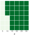

 % Time Spent on Data-
Related Computation
i.e., the proportion of total runtime that an algorithm spends computing the value, gradient, or Hessian of the loss function.
% Time Spent on Data-
Related Computation
i.e., the proportion of total runtime that an algorithm spends computing the value, gradient, or Hessian of the loss function.

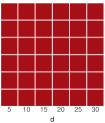
 Figure 27: Performance of MINLP algorithms on difficult instances of RiskSlimMINLP for synthetic datasets with varying dimensions and sample sizes . All algorithms perform similarly. We report results for ActiveSetMINLP in Section 3.3 because it solves the most instances to optimality.
E Additional Details on Algorithmic Improvements
E.1 Initialization Procedure
In Algorithm 7, we present an initialization procedure for LCPA. The procedure aims to speed up LCPA by generating: a collection of cutting planes; a good integer solution; and non-trivial bounds on the values of the objective, loss, and number of non-zero coefficients. It combines all of the techniques from this section, as follows: 1. Run CPA using RiskSlimLP: We apply traditional CPA to produce a cutting-plane approximation of the loss function using a convex relaxation of RiskSlimMINLP. We can achieve this by replacing in Step 12 of CPA with , and running CPA until a user-specified stopping condition is met. We store: (i) the cuts from RiskSlimLP (which will be used as an initial cutting plane approximation for LCPA); (ii) the lower bound from CPA on the objective value of RiskSlimLP (which represents a lower bound on the optimal value of RiskSlimMINLP). 2. Sequential Rounding and Polishing: We collect the solutions produced at each iteration of CPA. For each solution, we run SequentialRounding to obtain an integer solution for RiskSlimMINLP, and then polish it using DCD. We use the best solution found so far to update the upper bound on the optimal value to RiskSlimMINLP. 3. Chained Updates: Having obtained non-trivial bounds on and , we update the bounds on key quantities using ChainedUpdates. In Figure 28, we show how the initialization procedure in Algorithm 7 improves the lower bound and the optimality gap over the course of LCPA. Algorithm 7 Initialization Procedure for LCPA 1: 2: training data 3: coefficient set 4: penalty parameter 5:, , , , , initial bounds on , and 6: time limit for CPA on RiskSlimLP 7: 8: initial approximation of loss function 9: initial collection of integer solutions 10:I: Run CPA using subroutine RiskSlimLP 11:Run CPA Algorithm 1 using 12: number of cuts added by CPA within time limit 13: store cuts from each iteration 14: store solutions from each iteration 15: lower bound from CPA lower bound for RiskSlimLP is lower bound for RiskSlimMINLP 16:II: Round and Polish Non-Integer Solutions from CPA 17:for each do 18: Algorithm 4 19: Algorithm 3 20: store polished integer solutions 21:end for 22: 23: best integer solution produces upper bound for 24:III: Update Bounds on Objective Terms 25: Algorithm 5 26:, , , , , , ,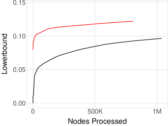
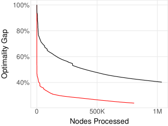 Figure 28: Performance profile of LCPA in a basic implementation (black) and with the initialization procedure in Algorithm 7 (red). Results reflect performance on a RiskSlimMINLP instance for a synthetic dataset with and 50,000 (see Appendix D for details).