Structure of attractors for boundary maps associated to Fuchsian groups

Abstract.

We study dynamical properties of generalized Bowen-Series boundary maps associated to cocompact torsion-free Fuchsian groups. These maps are defined on the unit circle (the boundary of the Poincaré disk) by the generators of the group and have a finite set of discontinuities. We study the two forward orbits of each discontinuity point and show that for a family of such maps the cycle property holds: the orbits coincide after finitely many steps. We also show that for an open set of discontinuity points the associated two-dimensional natural extension maps possess global attractors with finite rectangular structure. These two properties belong to the list of “good” reduction algorithms, equivalence or implications between which were suggested by Don Zagier [11].

1. Introduction

Let $\Gamma$ be a finitely generated Fuchsian group of the first kind acting on the hyperbolic plane. We will use either the upper half-plane model $\mathcal{H}$ or the unit disk model $\mathbb{D}$, and will denote the Euclidean boundary for either model by ${\mathbb{S}}$: for the upper half plane ${\mathbb{S}}=\partial(\mathcal{H})={\mathbb{P}}^{1}(\mathbb{R})$, and for the unit disk ${\mathbb{S}}=\partial(\mathbb{D})=\mathbf{S}^{1}$.

Let $\mathcal{F}$ be a fundamental domain for $\Gamma$ with an even number $N$ of sides identified by the set of generators $G=\{T_{1},\dots,T_{N}\}$ of $\Gamma$, and $\tau:{\mathbb{S}}\to G$ be a surjective map locally constant on ${\mathbb{S}}\setminus J$, where $J=\{x_{1},\dots,x_{N}\}$ is an arbitrary set of jumps. A boundary map $f:{\mathbb{S}}\to{\mathbb{S}}$ is defined by $f(x)=\tau(x)x$. It is a piecewise fractional-linear map whose set of discontinuities is $J$. Let $\Delta=\{(x,x)\mid x\in{\mathbb{S}}\}\subset{\mathbb{S}}\times{\mathbb{S}}$ be the diagonal of ${\mathbb{S}}\times{\mathbb{S}}$, and $F:{\mathbb{S}}\times{\mathbb{S}}\setminus\Delta\to{\mathbb{S}}\times{\mathbb{S}}\setminus\Delta$ be given by

$$F(x,y)=(\tau(y)x,\tau(y)y).$$

This is a (natural) extension of $f$, and if we identify $(x,y)\in{\mathbb{S}}\times{\mathbb{S}}\setminus\Delta$ with an oriented geodesic from $x$ to $y$, we can think of $F$ as a map on geodesics $(x,y)$ which we will also call a reduction map.

Several years ago Don Zagier[11] proposed a list of possible notions of “good” reduction algorithms associated to Fuchsian groups and conjectured equivalences or implications between them. In this paper we consider two of these notions, namely the properties that “good” reduction algorithms should (i) satisfy the cycle property, and (ii) have an attractor with finite rectangular structure. We prove that for each cocompact torsion-free Fuchsian group there exist families of reduction algorithms which satisfy these properties. Thus our results are contributions towards Zagier’s conjecture.

Although the statement that each Fuchsian group admits a “good” reduction algorithm is not part of Zagier’s conjecture, it is certainly related to it, and for the purposes of this paper, we state it here.

Reduction Theory Conjecture for Fuchsian groups

For every Fuchsian group $\Gamma$ there exist $\mathcal{F},G$ as above, and an open set of $J^{\prime}s$ in ${\mathbb{S}}^{N}$ such that

1. The map $F$ possesses a bijectivity domain $\Omega$ having a finite rectangular structure, i.e., bounded by non-decreasing step-functions with a finite number of steps.

2. Every point $(x,y)\in{\mathbb{S}}\times{\mathbb{S}}\setminus\Delta$ is mapped to $\Omega$ after finitely many iterations of $F$.

Remark 1.1.

If property (2) holds, then $\Omega$ is a global attractor for the map $F$, i.e.

(1.1) $$\Omega=\bigcap_{n=0}^{\infty}F^{n}({\mathbb{S}}\times{\mathbb{S}}\setminus\Delta).$$

This conjecture was proved by the authors in [6] for $\Gamma=SL(2,\mathbb{Z})$ and boundary maps associated to $(a,b)$-continued fractions. Notice that for some classical cases of continued fraction algorithms property (2) holds only for almost every point, while property (1.1) remains valid.

In this paper we address the conjecture for surface groups. In the Poincaré unit disk model $\mathbb{D}$ endowed with the hyperbolic metric

(1.2) $$\frac{2|dz|}{1-|z|^{2}},$$

let $\Gamma$ be a Fuchsian group, i.e. a discrete group of orientation preserving isometries of $\mathbb{D}$, acting freely on $\mathbb{D}$ with $\Gamma\backslash\mathbb{D}$ compact domain. Such $\Gamma$ is called a surface group, and the quotient $\Gamma\backslash\mathbb{D}$ is a compact surface of constant negative curvature $-1$ of a certain genus $g>1$. A classical (Ford) fundamental domain for $\Gamma$ is a $4g$-sided regular polygon centered at the origin (see a sketch of the construction in [5] in the manner of [4], and for the complete proof see [8]). A more suitable for our purposes $(8g-4)$-sided fundamental domain $\mathcal{F}$ was described by Adler and Flatto in [1]. They showed that all angles of $\mathcal{F}$ are equal to $\frac{\pi}{2}$ and, therefore, its sides are geodesic segments which satisfy the extension condition of Bowen and Series [3]: the geodesic extensions of these segments never intersect the interior of the tiling sets $\gamma\mathcal{F}$, $\gamma\in\Gamma$. Figure 1 shows such a construction for $g=2$.

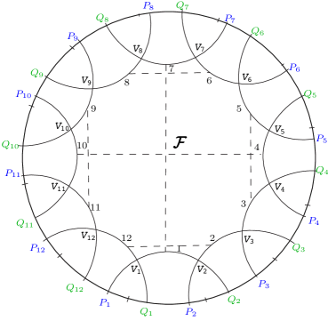
Figure 1. The fundamental domain $\mathcal{F}$ for a genus $2$ surface

Using notations similar to [1], we label the sides of $\mathcal{F}$ in a counterclockwise order by numbers $1\leq i\leq 8g-4$, as they are arcs of the corresponding isometric circles of generators $T_{i}$. We denote the corresponding vertices of $\mathcal{F}$ by $V_{i}$, so that the side $i$ connects the vertices $V_{i}$ and $V_{i+1}\pmod{8g-4}$. The identification of the sides is given by the pairing rule:

$$\sigma(i)=\begin{cases}4g-i\mod(8g-4)\text{ for odd }i\\ 2-i\mod(8g-4)\text{ for even }i\end{cases}\,.$$

The generators $T_{i}$ associated to this fundamental domain are Möbius transformations satisfying the following properties:

(1.3) $$T_{\sigma(i)}T_{i}=Id$$

(1.4) $$T_{i}(V_{i})=V_{\rho(i)},\text{ where }\rho(i)=\sigma(i)+1$$

(1.5) $$T_{\rho^{3}(i)}T_{\rho^{2}(i)}T_{\rho(i)}T_{i}=Id$$

We denote by $P_{i}Q_{i+1}$ the oriented (infinite) geodesic that extends the side $i$ to the boundary of the fundamental domain $\mathcal{F}$. It is important to remark that ${P_{i}Q_{i+1}}$ is the isometric circle for $T_{i}$, and $T_{i}\left({P_{i}Q_{i+1}}\right)={Q_{\sigma(i)+1}P_{\sigma(i)}}$ is the isometric circle for $T_{\sigma(i)}$ so that the inside of the former isometric circle is mapped to the outside of the latter.

The counter-clockwise order of theses points on ${\mathbb{S}}$ is

(1.6) $$P_{1},Q_{1},P_{2},Q_{2},\dots,P_{8g-4},Q_{8g-4},P_{1}.$$

Bowen and Series [3] defined the boundary map $f_{\bar{P}}:{\mathbb{S}}\rightarrow{\mathbb{S}}$

(1.7) $$f_{\bar{P}}(x)=T_{i}(x)\quad\text{if }P_{i}\leq x<P_{i+1}\,.$$

with the set of jumps $J=\bar{P}=\{P_{1},\dots,P_{8g-4}\}$. They showed that such a map is Markov with respect to the partition (1.6), expanding, and satisfies Rényi’s distortion estimates, hence it admits a unique finite invariant ergodic measure equivalent to Lebesgue measure.

Adler and Flatto [1] proved the existence of an invariant domain for the corresponding natural extension map $F_{\bar{P}}$, $\Omega_{\bar{P}}\subset{\mathbb{S}}\times{\mathbb{S}}$. Moreover, the set $\Omega_{\bar{P}}$ they identified has a regular geometric structure, what we call finite rectangular (see Figure 2, with $\Omega_{\bar{P}}$ shown as a subset of $[-\pi,\pi]^{2}$). The maps $F_{\bar{P}}$ and $f_{\bar{P}}$ are ergodic. Both Series [9] and Adler-Flatto [1] explain how the boundary map can be used for coding symbolically the geodesic flow on $\mathbb{D}/\Gamma$.

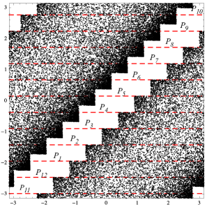
Figure 2. Domain of the Bowen-Series map $F_{\bar{P}}$ as a subset of $[-\pi,\pi]^{2}$

Notations. For $A,B\in{\mathbb{S}}$, the various intervals on ${\mathbb{S}}$ between $A$ and $B$ (with the counterclockwise order) will be denoted by $[A,B],(A,B],[A,B)$ and $(A,B)$. The geodesic (segment) from a point $C\in{\mathbb{S}}$ (or $\mathbb{D}$) to $D\in{\mathbb{S}}$ (or $\mathbb{D})$ will be denoted by $CD$.

Our object of study is a generalization of the Bowen-Series boundary map. We consider an open set of jumps

$$J=\bar{A}=\{A_{1},\dots,A_{8g-4}\}$$

with the only condition $A_{i}\in(P_{i},Q_{i})$, and define $f_{\bar{A}}:{\mathbb{S}}\rightarrow{\mathbb{S}}$ by

(1.8) $$f_{\bar{A}}(x)=T_{i}(x)\quad\text{if }A_{i}\leq x<A_{i+1}\,,$$

and the corresponding two-dimensional map:

(1.9) $$F_{\bar{A}}(x,y)=(T_{i}(x),T_{i}(y))\quad\text{if }A_{i}\leq y<A_{i+1}\,.$$

A key ingredient in analyzing map $F_{\bar{A}}$ is what we call the cycle property of the partition points $\{A_{1},\dots,A_{8g-4}\}$. Such a property refers to the structure of the orbits of each $A_{i}$ that one can construct by tracking the two images $T_{i}A_{i}$ and $T_{i-1}A_{i}$ of these points of discontinuity of the map $f_{\bar{A}}$. It happens that some forward iterates of these two images $T_{i}A_{i}$ and $T_{i-1}A_{i}$ under $f_{\bar{A}}$ coincide. This is another property from Zagier’s list of “good” reduction algorithms.

We state the cycle property result below and provide a proof in Section 3.

Theorem 1.2 (Cycle Property).

Each partition point $A_{i}\in(P_{i},Q_{i})$, $1\leq i\leq 8g-4$, satisfies the cycle property, i.e., there exist positive integers $m_{i},k_{i}$ such that

$$f_{\bar{A}}^{m_{i}}(T_{i}A_{i})=f_{\bar{A}}^{k_{i}}(T_{i-1}A_{i}).$$

If a cycle closes up after one iteration

(1.10) $$f_{\bar{A}}(T_{i}A_{i})=f_{\bar{A}}(T_{i-1}A_{i}),$$

we say that the point $A_{i}$ satisfies the short cycle property. Under this condition, we prove the following:

Theorem 1.3 (Main Result).

If each partition point $A_{i}$ satisfies the short cycle property (1.10), then there exists a set $\Omega_{\bar{A}}\subset{\mathbb{S}}\times{\mathbb{S}}$ with the following properties:

1. $\Omega_{\bar{A}}$ has a finite rectangular structure, and $F_{\bar{A}}$ is (essentially) bijective on $\Omega_{\bar{A}}$.

2. Almost every point $(x,y)\in{\mathbb{S}}\times{\mathbb{S}}\setminus\Delta$ is mapped to $\Omega_{\bar{A}}$ after finitely many iterations of $F_{\bar{A}}$, and $\Omega_{A}$ is a global attractor for the map $F_{\bar{A}}$, i.e.,

   $$\Omega_{A}=\bigcap_{n=0}^{\infty}F_{\bar{A}}^{n}({\mathbb{S}}\times{\mathbb{S}}\setminus\Delta).$$

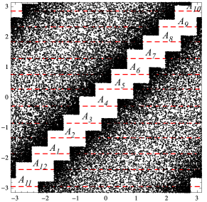
Figure 3. Domain (and attractor) of the generalized Bowen-Series map $F_{\bar{A}}$

Notice that the set of partitions satisfying the short cycle property contains an open set with this property, as explained in Remark 3.11. Thus we prove the Reduction Theory Conjecture. We believe that this result is true in greater generality, i.e., for all partitions $\bar{A}=\{A_{i}\}$ with $A_{i}\in(P_{i},Q_{i})$.

Organization of the paper

In Section 2 we prove properties (1) and (2) of the Reduction Theory Conjecture for the classical Bowen-Series case when the partition points are given by the set $\bar{P}=\{P_{i}\}$. In Section 3 we prove the cycle property for any partition $\bar{A}=\{A_{i}\}$ with $A_{i}\in(P_{i},Q_{i})$. In Section 4 we determine the structure of the set $\Omega_{\bar{A}}$ in the case when the partition $\bar{A}$ satisfies the short cycle property and prove the bijectivity of the map $F_{\bar{A}}$ on $\Omega_{\bar{A}}$. In Section 5 we identify the trapping region for the map $F_{\bar{A}}$ and prove that every point in ${\mathbb{S}}\times{\mathbb{S}}\setminus\Delta$ is mapped to it after finitely many iterations of the map $F_{\bar{A}}$. And finally, in Section 6 we prove that almost every point ${\mathbb{S}}\times{\mathbb{S}}\setminus\Delta$ is mapped to $\Omega_{\bar{A}}$ after finitely many iterations of the map $F_{\bar{A}}$ and complete the proof of Theorem 1.3. In Section 7 we apply our results to calculate the invariant probability measures for the maps $F_{\bar{A}}$ and $f_{\bar{A}}$.

2. Bowen-Series case

In this section we prove properties (1) and (2) of the Reduction Theory Conjecture for the Bowen-Series classical case, where the partition $\bar{A}$ is given by the set of points $\bar{P}=\{P_{1},\dots,P_{8g-4}\}$.

Theorem 2.1.

The two-dimensional Bowen-Series map $F_{\bar{P}}$ satisfies properties (1) and (2) of the Reduction Theory Conjecture.

Before we prove this theorem, we state a useful proposition that can be easily derived using the isometric circles and the conformal property of Möbius transformations (see also Theorem 3.4 of [1]).

Proposition 2.2.

$T_{i}$ maps the points $P_{i-1}$, $P_{i}$, $Q_{i}$, $P_{i+1}$, $Q_{i+1}$, $Q_{i+2}$ respectively to $P_{\sigma(i)+1}$, $Q_{\sigma(i)+1}$, $Q_{\sigma(i)+2}$, $P_{\sigma(i)-1}$, $P_{\sigma(i)}$, $Q_{\sigma(i)}$.

Proof of Theorem 2.1.

In this case the set $\Omega_{\bar{P}}$ is determined by the corner points located in each horizontal strip

$$\{(x,y)\in{\mathbb{S}}\times{\mathbb{S}}\mid y\in[P_{i},P_{i+1})\}$$

(see Figure 4) with coordinates

$$(P_{i},Q_{i})\text{ (upper part)}\;\text{ and }\;(Q_{i+2},P_{i+1})\text{ (lower part)}.$$

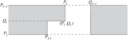
Figure 4. Strip $y\in[P_{i},P_{i+1}]$ of $\Omega_{\bar{P}}$

This set obviously has a finite rectangular structure. One can also verify immediately the essential bijectivity, by investigating how different regions of $\Omega_{\bar{P}}$ are mapped by $F_{\bar{P}}$. More precisely we look at the strip $S_{i}$ of $\Omega_{\bar{P}}$ given by $y\in[P_{i},P_{i+1}]$, and its image under $F_{\bar{P}}$, in this case $T_{i}$.

We consider the following decomposition of this strip: $\tilde{S}_{i}=[Q_{i+2},P_{i-1}]\times[P_{i},Q_{i}]$ (red rectangular horizontal piece), $\hat{S}_{i}=[Q_{i+2},P_{i}]\times[Q_{i},P_{i+1}]$ (green horizontal rectangular piece). Now

$$T_{i}(\tilde{S}_{i}) =[T_{i}Q_{i+2},T_{i}P_{i-1}]\times[T_{i}P_{i},T_{i}Q_{i}]=[Q_{\sigma(i)},P_{\sigma(i)+1}]\times[Q_{\sigma(i)+1},Q_{\sigma(i)+2}]$$

$$T_{i}(\hat{S}_{i}) =[T_{i}Q_{i+2},T_{i}P_{i}]\times[T_{i}Q_{i},T_{i}P_{i+1}]=[Q_{\sigma(i)},Q_{\sigma(i)+1}]\times[Q_{\sigma(i)+2},P_{\sigma(i)-1}]$$

Therefore $T_{i}(S_{i})$ is a complete vertical strip in $\Omega_{\bar{P}}$, with $Q_{\sigma(i)}\leq x\leq Q_{\sigma(i)+1}$. This completes the proof of the property (1).

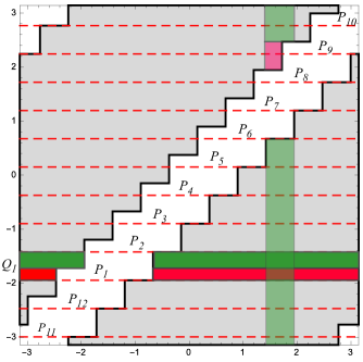
Figure 5. Bijectivity of the Bowen-Series map $F_{\bar{P}}$

We now prove property (2) for the set $\Omega_{P}$.

Consider $(x,y)\in{\mathbb{S}}\times{\mathbb{S}}\setminus\Delta$. Notice that there exists $n(x,y)>0$ such that the two values $x_{n},y_{n}$ obtained from the $n$th iterate of $F_{\bar{P}}$, $(x_{n},y_{n})=F^{n}_{\bar{P}}(x,y)$, are not inside the same isometric circle; in other words, $(x_{n},y_{n})\not\in X_{i}=[P_{i},Q_{i+1}]\times[P_{i},P_{i+1})$ for all $1\leq i\leq 8g-4$. Indeed, if one assumes that both coordinates $(x_{n},y_{n})=F^{n}_{\bar{P}}(x,y)$ belong to such a set $X_{i}$ for all $n\geq 0$, each time we iterate the pair $(x_{n},y_{n})$ we apply one of the maps $T_{i}$ which is expanding in the interior of its isometric circle. Thus the distance between $x_{n}$ and $y_{n}$ would grow sufficiently for the points to be inside different isometric circles. Therefore, there exists $n>0$ such that $y_{n}$ is in some interval $[P_{i},P_{i+1})\subset[P_{i},Q_{i+1}]$ and $x_{n}\not\in[P_{i},Q_{i+1}]$.

Notice that, from the definition of $\Omega_{\bar{P}}$, in order to prove the attracting property, we need to analyze the situations $(x_{n},y_{n})\in[P_{i-1},P_{i}]\times[P_{i},Q_{i}]$ and $(x_{n},y_{n})\in[Q_{i+1},Q_{i+2}]\times[P_{i},P_{i+1})$ and show that a forward iterate lands in $\Omega_{\bar{P}}$.

Case I. If $(x_{n},y_{n})\in[Q_{i+1},Q_{i+2}]\times[P_{i},P_{i+1})$, then

$$F_{\bar{P}}(x_{n},y_{n})\in[T_{i}Q_{i+1},T_{i}Q_{i+2}]\times[T_{i}P_{i},T_{i}P_{i+1})=[P_{\sigma(i)},Q_{\sigma(i)}]\times[Q_{\sigma(i)+1},P_{\sigma(i)-1}).$$

The subset $[P_{\sigma(i)},Q_{\sigma(i)}]\times[Q_{\sigma(i)+1},P_{\sigma(i)-2}]$ is included in $\Omega_{\bar{P}}$ so we only need to analyze the situation $(x_{n+1},y_{n+1})\in[P_{k+2},Q_{k+2}]\times[P_{k},P_{k+1})$, where $k=\sigma(i)-2$. Then

$$(x_{n+2},y_{n+2})=F^{2}_{P}(x_{n},y_{n})=T_{k}T_{i}(x_{n},y_{n})\in[T_{k}P_{k+2},Q_{\sigma(k)}]\times[Q_{\sigma(k)+1},P_{\sigma(k)-1})\,.$$

Notice that $T_{k}P_{k+2}\in[P_{\sigma(k)},Q_{\sigma(k)}]$. The subset $[T_{k}P_{k+2},Q_{\sigma(k)}]\times[Q_{\sigma(k)+1},P_{\sigma(k)-2}]$ is included in $\Omega_{\bar{P}}$ so we only need to analyze the situation

$$(x_{n+2},y_{n+2})\in[T_{k}P_{k+2},Q_{\sigma(k)}]\times[P_{\sigma(k)-2},P_{\sigma(k)-1})\subset[P_{\sigma(k)},Q_{\sigma(k)}]\times[P_{\sigma(k)-2},P_{\sigma(k)-1}).$$

Notice that $\sigma(k)-2=\sigma(\sigma(i)-2)-2=i$ (direct verification), so we are back to analyzing the situation $(x_{n+2},y_{n+2})\in[P_{i+2},Q_{i+2}]\times[P_{i},P_{i+1})$. The boundary map $f_{\bar{P}}$ is expanding, so it is not possible for the images of the interval $(y_{n},P_{i+1})$ (on the $y$-axis) to alternate indefinitely between the intervals $[P_{i},P_{i+1}]$ and $[P_{\sigma(i)-2},P_{\sigma(i)-1}]$, where $T_{i}P_{i+1}=P_{\sigma(i)-1}$.

This means that either some even iterate

$$F^{2m}(x_{n},y_{n})\in[P_{i+2},Q_{i+2}]\times[Q_{i+3},P_{i})\subset\Omega_{\bar{P}}$$

or some odd iterate

$$F^{2m+1}(x_{n},y_{n})\in[P_{\sigma(i)},Q_{\sigma(i)}]\times[Q_{\sigma(i)+1},P_{\sigma(i)-2}]\subset\Omega_{\bar{P}}.$$

Case II. If $(x_{n},y_{n})\in[P_{i-1},P_{i}]\times[P_{i},Q_{i}]$, then

$$F_{\bar{P}}(x_{n},y_{n})\in[T_{i}P_{i-1},T_{i}P_{i}]\times[T_{i}P_{i},T_{i}Q_{i}]=[P_{\sigma(i)+1},Q_{\sigma(i)+1}]\times[Q_{\sigma(i)+1},Q_{\sigma(i)+2}]\,.$$

There are two subcases that we need to analyze:

$$(a)\;\;(x_{n+1},y_{n+1})\in[P_{k},Q_{k}]\times[Q_{k},P_{k+1})\quad(b)\;\;(x_{n+1},y_{n+1})\in[P_{k},Q_{k}]\times[P_{k+1},Q_{k+1}],$$

where $k=\sigma(i)+1$.

Case (a) If $(x_{n+1},y_{n+1})\in[P_{k},Q_{k}]\times[Q_{k},P_{k+1}]$, then

$$(x_{n+2},y_{n+2})\in T_{k}\left([P_{k},Q_{k}]\times[Q_{k},P_{k+1})\right)=[Q_{\sigma(k)+1},Q_{\sigma(k)+2}]\times[Q_{\sigma(k)+2},P_{\sigma(k)-1}]\,.$$

Notice that $\sigma(k)+1=\sigma(\sigma(i)+1)+1=4g+i-2$ (direct verification), so when analyzing the situation $(x_{n+2},y_{n+2})\in[Q_{4g+i-2},Q_{4g+i-1}]\times[Q_{4g+i-1},P_{4g+i-4})$ the only problematic region is $(x_{n+2},y_{n+2})\in[P_{4g+i-1},Q_{4g+i-1}]\times[Q_{4g+i-1},Q_{4g+i}]$.

Case (b) If $(x_{n+1},y_{n+1})\in[P_{k},Q_{k}]\times[P_{k+1},Q_{k+1}]$, then

$$(x_{n+2},y_{n+2}) \in T_{k+1}\left([P_{k},Q_{k}]\times[P_{k+1},Q_{k+1}]\right)$$

$$=[P_{\sigma(k+1)+1},T_{k+1}Q_{k}]\times[Q_{\sigma(k+1)+1},Q_{\sigma(k+1)+2}].$$

Notice that $T_{k+1}Q_{k}\in[P_{\sigma(k+1)+1},Q_{\sigma(k+1)+1}]$ and $\sigma(k+1)+1=i-1$ (direct verification) so we are left to investigate $(x_{n+2},y_{n+2})\in[P_{i-1},Q_{i-1}]\times[Q_{i-1},Q_{i}]$.

To summarize, we started with $(x_{n+1},y_{n+1})\in[P_{\sigma(i)+1},Q_{\sigma(i)+1}]\times[Q_{\sigma(i)+1},Q_{\sigma(i)+2}]\,$ and found two situations that need to be analyzed: $(x_{n+2},y_{n+2})\in[P_{i-1},Q_{i-1}]\times[Q_{i-1},Q_{i}]$ and $(x_{n+2},y_{n+2})\in[P_{4g+i-1},Q_{4g+i-1}]\times[Q_{4g+i-1},Q_{4g+i}]$.

We prove in what follows that it is not possible for all future iterates $F^{m}(x_{n},y_{n})$ to belong to the sets of type $[P_{k},Q_{k}]\times[Q_{k},Q_{k+1}]$. First, it is not possible for all $F^{m}(x_{n},y_{n})$ (starting with some $m>0$) to belong only to type-a sets $[P_{k_{m}},Q_{k_{m}}]\times[Q_{k_{m}},P_{k_{m}+1}]$, where the sequence $\{k_{m}\}$ is defined recursively as $k_{m}=\sigma(k_{m-1})+2$, because such a set is included in the isometric circle $X_{k_{m}}$, and the argument at the beginning of the proof disallows such a situation.

Also, it is not possible for all $F^{m}(x_{n},y_{n})$ (starting with some $m>0$) to belong only to type-b sets $[P_{k_{m}},Q_{k_{m}}]\times[P_{k_{m}+1},Q_{k_{m}+1}]$, where $k_{m}=\sigma(k_{m-1}+1)+1$: this would imply that the pairs of points $(y_{n+m},Q_{k_{n+m}+1})$ (on the $y$-axis) will belong to the same interval $[P_{k_{n+m}+1},Q_{k_{n+m}+1}]$ which is impossible due to expansiveness property of the map $f_{\bar{P}}$. Therefore, there exists a pair $(x_{l},y_{l})$ in the orbit of $F^{m}(x_{n},y_{n})$ such that

$$(x_{l},y_{l})\in[P_{j},Q_{j}]\times[P_{j+1},Q_{j+1}]\text{ (type-b)}$$

for some $1\leq j\leq 8g-4$ and

$$(x_{l+1},y_{l+1})\in[P_{j^{\prime}},T_{j+1}Q_{j}]\times[Q_{j^{\prime}},P_{j^{\prime}+1}]\subset[P_{j^{\prime}},Q_{j^{\prime}}]\times[Q_{j^{\prime}},P_{j^{\prime}+1}]\text{ (type-a)},$$

where $j^{\prime}=\sigma(j+1)+1$. Then

$$(x_{l+2},y_{l+2})\in T_{j^{\prime}}([P_{j^{\prime}},T_{j+1}Q_{j}]\times[Q_{j^{\prime}},P_{j^{\prime}+1}])=[Q_{j^{\prime\prime}},T_{j^{\prime}}T_{j+1}Q_{j}]\times[Q_{j^{\prime\prime}+1},P_{j^{\prime\prime}-2}]$$

where $j^{\prime\prime}=\sigma(j^{\prime})+1$.

Using the results of the Appendix (Corollary 8.3), we have that the arc length distance

$$\ell(P_{j^{\prime}},T_{j+1}Q_{j})=\ell(T_{j+1}P_{j},T_{j+1}Q_{j})<\frac{1}{2}\ell(P_{j^{\prime}},Q_{j^{\prime}}).$$

Now we can use Corollary 8.2 (ii) applied to the point $T_{j+1}Q_{j}\in[P_{j^{\prime}},Q_{j^{\prime}}]$ to conclude that $T_{j^{\prime}}T_{j+1}Q_{j}\in[Q_{j^{\prime\prime}},P_{j^{\prime\prime}+1}]$. Therefore $(x_{l+2},y_{l+2})\in\Omega_{\bar{P}}$. This completes the proof of the property (2). ∎

Remark 2.3.

One can prove along the same lines that if the partition $\bar{A}$ is given by the set $\bar{Q}=\{Q_{1},\dots,Q_{8g-4}\}$, the properties (1) and (2) of the Reduction Theory Conjecture also hold.

3. The cycle property

The map $f_{\bar{A}}$ is discontinuous at $x=A_{i}$, $1\leq i\leq 8g-4$. We associate to each point $A_{i}$ two forward orbits: the upper orbit ${\mathcal{O}}_{u}(A_{i})=\{f_{\bar{A}}^{n}(T_{i}A_{i})\}_{n\geq 0}$, and the lower orbit ${\mathcal{O}}_{\ell}(A_{i})=\{f_{\bar{A}}^{n}(T_{i-1}A_{i})\}_{n\geq 0}$. We use the convention that if an orbit hits one of the discontinuity points $A_{j}$, then the next iterate is computed according to the left or right location: for example, if the lower orbit of $A_{i}$ hits some $A_{j}$, then the next iterate will be $T_{j-1}A_{j}$, and if the upper orbit of $A_{i}$ hits some $A_{j}$ then the next iterate is $T_{j}A_{j}$.

Now we explore the patterns in the above orbits. The following property plays an essential role in studying the maps $f_{\bar{A}}$ and $F_{\bar{A}}$.

Definition 3.1.

We say that the point $A_{i}$ has the cycle property if for some non-negative integers $m_{i},k_{i}$

$$f_{\bar{A}}^{m_{i}}(T_{i}A_{i})=f_{\bar{A}}^{k_{i}}(T_{i-1}A_{i})=:c_{A_{i}}.$$

We will refer to the set

$$\{T_{i}A_{i},f_{\bar{A}}T_{i}A_{i},\dots,f_{\bar{A}}^{m_{i}-1}T_{i}A_{i}\}$$

as the upper side of the $A_{i}$-cycle, the set

$$\{T_{i-1}A_{i},f_{\bar{A}}T_{i-1}A_{i},\dots,f_{\bar{A}}^{k_{i}-1}T_{i-1}A_{i}\}$$

as the lower side of the $A_{i}$-cycle, and to $c_{A_{i}}$ as the end of the $A_{i}$-cycle.

The main goal of this section is to prove Theorem 1.2 (cycle property) stated in the Introduction. First, we prove some preliminary results.

Lemma 3.2.

The following identity holds

(3.1) $$T_{\sigma(i)+1}T_{i}=T_{\sigma(i-1)-1}T_{i-1}$$

Proof.

Using relation (1.5) stated in the Introduction, we have that

$$T_{\rho(i)}T_{i}=T^{-1}_{\rho^{2}(i)}T^{-1}_{\rho^{3}(i)}$$

(where $\rho(i)=\sigma(i)+1$), so it is enough to show that $T^{-1}_{\rho^{2}(i)}=T_{\sigma_{i-1}-1}$ and $T^{-1}_{\rho^{3}(i)}=T_{i-1}$. For that we analyze the two parity cases.

If $i$ is odd, we have the following identities $\!\!\mod(8g-4)$:

$$\rho(i) =\sigma(i)+1=4g-i+1\text{ (even)}$$

$$\rho^{2}(i) =\sigma(4g-i+1)+1=2-(4g-i+1)+1=2-4g+i=4g-2+i\text{ (odd)}$$

$$\rho^{3}(i) =\sigma(2-4g+i)+1=4g-(2-4g+i)+1=8g-1-i=3-i\text{ (even)}$$

Since $\sigma(i-1)=3-i=\rho^{3}(i)$, one has $T^{-1}_{\rho^{3}(i)}=T_{i-1}$ by using (1.4). Also, $\sigma(i-1)-1=2-(i-1)-1=2-i$ and $\sigma(\rho^{2}(i))=2-i$, hence $T^{-1}_{\rho^{2}(i)}=T_{\sigma(i-1)-1}$.

If $i$ is even, we have the following identities $\!\!\mod(8g-4)$:

$$\rho(i) =\sigma(i)+1=3-i\text{ (odd)}$$

$$\rho^{2}(i) =\sigma(3-i)+1=4g-(3-i)+1=4g-2+i\text{ (even)}$$

$$\rho^{3}(i) =\sigma(4g-2+i)+1=2-(4g-2+i)+1=5-4g-i=4g+1-i\text{ (odd)}$$

Since $\sigma(i-1)=4g-(i-1)=\rho^{3}(i)$, one has $T^{-1}_{\rho^{3}(i)}=T_{i-1}$ by using (1.4). Also, $\sigma(i-1)-1=4g-i$ and $\sigma(\rho^{2}(i))=4g-i$, hence $T^{-1}_{\rho^{2}(i)}=T_{\sigma(i-1)-1}$.

Identity (3.1) has been proved for both cases. ∎

Remark 3.3.

By introducing the notation $\theta(i)=\sigma(i)-1$, relation (3.1) can be written

(3.2) $$T_{\rho(i)}T_{i}=T_{\theta(i-1)}T_{i-1},$$

which will simplify further calculations.

Lemma 3.4.

For any $1\leq i\leq 8g-4$, $\theta(\theta(i-1)-1))=i$ and $\rho(\rho(i)+1)+1=i$.

Proof.

Immediate verification. ∎

Lemma 3.5.

The relations $f^{2}_{\bar{A}}(P_{i})=P_{i}$ and $f^{2}_{\bar{A}}(Q_{i})=Q_{i}$ hold for all $i$. In addition, $f_{\bar{A}}(P_{i})=P_{i}$ if $i\in\{1,2g,4g-1,6g-2\}$, and $f_{\bar{A}}(Q_{i})=Q_{i}$ if $i\in\{2,2g+1,4g,6g-1\}$.

Proof.

We have

$$f^{2}_{\bar{A}}(P_{i})=f_{\bar{A}}(T_{i-1}P_{i})=f_{\bar{A}}(P_{\theta(i-1)})=P_{\theta(\theta(i-1)-1)}=P_{i}$$

and

$$f^{2}_{\bar{A}}(Q_{i})=f_{\bar{A}}(T_{i}Q_{i})=f_{\bar{A}}(Q_{\rho(i)+1})=Q_{\rho(\rho(i)+1)+1}=Q_{i}$$

by Lemma 3.4. The second part follows easily, too. ∎

Proof of Theorem 1.2.

Let us analyze the upper and lower orbits of $A_{i}$. By Proposition 2.2 and the orientation preserving property of the Möbius transformations, we have

(3.3) $$T_{i}[P_{i},Q_{i}]=[Q_{\rho(i)},Q_{\rho(i)+1}],\quad T_{i-1}[P_{i},Q_{i}]=[P_{\theta(i-1)},P_{\theta(i-1)+1}],$$

therefore

(3.4) $$T_{i}A_{i}\in\left(Q_{\rho(i)},Q_{\rho(i)+1}\right)\;,\;T_{i-1}A_{i}\in\left(P_{\theta(i-1)},P_{\theta(i-1)+1}\right)$$

Depending on whether $T_{i}A_{i}\in(Q_{\rho(i)},A_{\rho(i)+1})$ or $T_{i}A_{i}\in{[}A_{\rho(i)+1},Q_{\rho(i)+1})$ we have either

$$f_{\bar{A}}(T_{i}A_{i})=T_{\rho(i)}T_{i}A_{i}\text{ or }f_{\bar{A}}(T_{i}A_{i})=T_{\rho(i)+1}T_{i}A_{i}\,.$$

Also, depending on whether $T_{i-1}A_{i}\in(P_{\theta(i-1)},A_{\theta(i-1)}{]}$ or $T_{i-1}A_{i}\in(A_{\theta(i-1)},P_{\theta(i-1)+1})$ we have either

$$f_{\bar{A}}(T_{i-1}A_{i})=T_{\theta(i-1)-1}T_{i-1}A_{i}\text{ or }f_{\bar{A}}(T_{i-1}A_{i})=T_{\theta(i-1)}T_{i}A_{i}\,.$$

Notice that in the case when $T_{i}A_{i}\in(Q_{\rho(i)},A_{\rho(i)+1})$ and $T_{i-1}A_{i}\in(A_{\theta(i-1)},P_{\theta(i-1)+1})$ the cycle property holds immediately with $m_{i}=k_{i}=1$, by using relation (3.2).

We are left to analyze the cases $T_{i}A_{i}\in[A_{\rho(i)+1},Q_{\rho(i)+1})$ or $T_{i-1}A_{i}\in(P_{\theta(i-1)},A_{\theta(i-1)}]$.

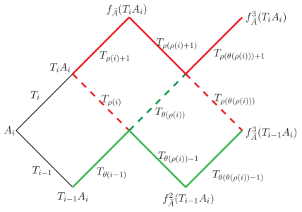
Figure 6. The first iterates of the upper and lower orbits of $A_{i}$

Lemma 3.6.

Given $x\in(P_{i},Q_{i})$ then one cannot have $T_{i}x\in[A_{\rho(i)+1},Q_{\rho(i)+1})$ and $T_{i-1}x\in(P_{\theta(i-1)},A_{\theta(i-1)}]$ simultaneously.

Proof.

Let $M_{i}$ be the midpoint of $(P_{i},Q_{i})$. By Corollary 8.2 of the Appendix, there exists $a_{i}\in(M_{i},Q_{i})$ such that $T_{i}(a_{i})=P_{\rho(i)+1}$ and $b_{i}\in(P_{i},M_{i})$ such that $T_{j-1}(b_{j})=Q_{\theta(j-1)}$.

Since $A_{\rho(i)+1}\in(P_{\rho(i)+1},Q_{\rho(i)+1})$ and $A_{\theta(i-1)}\in(P_{\theta(i-1)},Q_{\theta(i-1)}$, in order for $T_{i}x\in[A_{\rho(i)+1},Q_{\rho(i)+1})$, $x$ must be in $(a_{i},Q_{i})$, and in order for $T_{i-1}x\in(P_{\theta(i-1)},A_{\theta(i-1)}]$, $x$ must be in $(P_{i},b_{i})$. The lemma follows from the fact that these intervals are disjoint. ∎

Lemma 3.7.

 

• Assume $x\in[A_{j},Q_{j})$ and $T_{j-1}(x)\in(P_{\theta(j-1)},A_{\theta(j-1)}]$, then

  $$T_{\theta(j-1)-1}T_{j-1}(x)\in(x,P_{j+1}).$$

• Assume $x\in(P_{j},A_{j}]$ and $T_{j}(x)\in[A_{\rho(j)+1},Q_{\rho(j)+1})$, then

  $$T_{\rho(j)+1}T_{j}(x)\in(Q_{j-1},x).$$

Proof.

(i) Notice that $T_{\theta(j-1)-1}T_{j-1}(P_{j})=f^{2}_{\bar{A}}(P_{j})=P_{j}$ by Lemma 3.5. Also $T_{j-1}(x)\in(P_{\theta(j-1)},Q_{\theta(j-1)})$ therefore

$$T_{\theta(j-1)-1}T_{j-1}(x)\in T_{\theta(j-1)-1}(P_{\theta(j-1)},Q_{\theta(j-1)})=(P_{j},P_{j+1})$$

by (3.4) and the fact that $\theta(\theta(j-1)-1)=j$ by Lemma 3.4. It follows that

$$(T_{\theta(j-1)-1}T_{j-1})[P_{j},x]=[P_{j},T_{\theta(j-1)-1}T_{j-1}(x)]\subset[P_{j},P_{j+1}]\,.$$

Since $T_{\theta(j-1)-1}T_{j-1}$ expands $[P_{j},x]$ we get $T_{\theta(j-1)-1}T_{j-1}(x)\in(x,P_{j+1})$.

Part (ii) can be proved similarly. ∎

We continue the proof of the theorem and assume the situation

$$T_{i}A_{i}\in[A_{\rho(i)+1},Q_{\rho(i)+1}).$$

Lemma 3.6 implies that $T_{i-1}A_{i}{\notin}(P_{\theta(i-1)},A_{\theta(i-1)}]$, i.e. $T_{i-1}A_{i}\in(A_{\theta(i-1)},P_{\theta(i-1)+1})$. Notice that $f_{\bar{A}}(T_{i-1}A_{i})$ can be rewritten as $T_{\rho(i)}T_{i}A_{i}$ by Lemma 3.1, and the beginning of the two orbits of $A_{i}$ are given by

$${\mathcal{O}}_{u}(A_{i})=\{T_{i}A_{i},T_{\rho(i)+1}T_{i}A_{i},\dots\},\quad{\mathcal{O}}_{l}(A_{i})=\{T_{i-1}A_{i},T_{\rho(i)}T_{i}A_{i},\dots\}\,.$$

We can now apply Lemma 3.7 part (ii) for $x=A_{i}$ to obtain that

$$f_{\bar{A}}(T_{i}A_{i})=T_{\rho(i)+1}T_{i}A_{i}\in(Q_{i-1},A_{i}),$$

therefore $f^{2}_{\bar{A}}(T_{i}A_{i})=T_{\rho(\rho(i)+1)}T_{\rho(i)+1}(T_{i}A_{i})$ (recalling that $\rho(\rho(i)+1)=i-1$).

On the other hand $T_{\rho(i)}T_{i}A_{i}\in\left(P_{\theta(\rho(i))},P_{\theta(\rho(i))+1}\right)$. Depending on whether $T_{\rho(i)}T_{i}A_{i}\in\left(P_{\theta(\rho(i))},A_{\theta(\rho(i))}\right]$ or $T_{\rho(i)}T_{i}A_{i}\in\left(A_{\theta(\rho(i))},P_{\theta(\rho(i))+1}\right)$ we have that

$$f_{\bar{A}}(T_{\rho(i)}T_{i}A_{i})=T_{\theta(\rho(i))-1}(T_{\rho(i)}T_{i}A_{i})\text{ or }f_{\bar{A}}(T_{\rho(i)}T_{i}A_{i})=T_{\theta(\rho(i))}(T_{\rho(i)}T_{i}A_{i})\,.$$

In the latter case, the cycle property holds, by using relation (3.2): we have $f^{2}_{\bar{A}}(T_{i}A_{i})=f^{2}_{\bar{A}}(T_{i-1}A_{i})$, i.e.

$$T_{\rho(\rho(i)+1)}T_{\rho(i)+1}(T_{i}A_{i})=T_{\theta(\rho(i))}T_{\rho(i)}(T_{i}A_{i})\,.$$

We have

$$\begin{split}{\mathcal{O}}_{u}(A_{i})&=\{T_{i}A_{i},T_{\rho(i)+1}T_{i}A_{i},T_{\theta(\rho(i))}(T_{\rho(i)}T_{i}A_{i})\dots\}\\ {\mathcal{O}}_{l}(A_{i})&=\{T_{i-1}A_{i},T_{\rho(i)}T_{i}A_{i},T_{\theta(\rho(i)-1{)}}(T_{\rho(i)}T_{i}A_{i})\dots\}\,.\end{split}$$

Proposition 3.8.

Assume that $T_{i}A_{i}\in[A_{\rho(i)+1},Q_{\rho(i)+1})$, and $A_{i}$ does not satisfy the cycle property up to iteration $2M+2$. Let $\psi_{n}=(\theta\circ\rho)^{n}$. Then, for any $0\leq n\leq M$,

(3.5) $$\begin{split}&f_{\bar{A}}^{2n}(T_{i}A_{i})\in[A_{\rho(\psi_{n}(i))+1},Q_{\rho(\psi_{n}(i))+1})\\ &f_{\bar{A}}^{2n+1}(T_{i}A_{i})=T_{\rho(\psi_{n}(i))+1}(f_{\bar{A}}^{2n}(T_{i}A_{i}))\\ &f_{\bar{A}}^{2n+1}(T_{i-1}A_{i})=T_{\theta(\psi_{n}(i)-1)}(f_{\bar{A}}^{2n}(T_{i-1}A_{i}))=T_{\rho(\psi_{n}(i))}(f_{\bar{A}}^{2n}(T_{i}A_{i}))\end{split}$$

(3.6) $$\begin{split}&f_{\bar{A}}^{2n+1}(T_{i-1}A_{i})\in(P_{\psi_{n+1}(i)},A_{\psi_{n+1}(i)}]\\ &f_{\bar{A}}^{2n+2}(T_{i}A_{i})=T_{\rho(\psi_{n}(i))+1}(f_{\bar{A}}^{2n+1}(T_{i}A_{i}))=T_{\psi_{n+1}(i)}(f_{\bar{A}}^{2n+1}(T_{i-1}A_{i}))\\ &f_{\bar{A}}^{2n+2}(T_{i-1}A_{i})=T_{\psi_{n+1}(i)-1}(f_{\bar{A}}^{2n+1}(T_{i-1}A_{i}))\end{split}$$

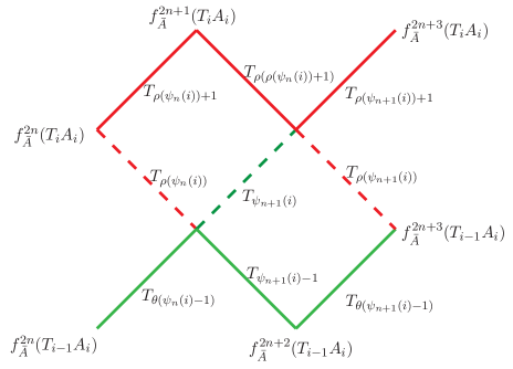
Figure 7. Iterates of upper and lower orbits of $A_{i}$

Proof.

We prove this by induction. The case $n=0$ has been already presented above ($\psi_{0}(i)=i$). Assume now that the relations are true for $k=1,2,\dots,n<M$. We analyze the case $k=n+1$. Let $\ell=\psi_{n}(i)$. First, notice that

$$\begin{split}f_{\bar{A}}^{2n+2}(T_{i-1}A_{i})&=T_{\psi_{n+1}(i)-1}(f_{\bar{A}}^{2n+1}(T_{i-1}A_{i}))=T_{\psi_{n+1}(i)-1}T_{\rho(\psi_{n}(i))}(f_{\bar{A}}^{2n}(T_{i}A_{i}))\\ &=T_{\theta(\rho(\ell))-1}T_{\rho(\ell)}(f_{\bar{A}}^{2n}(T_{i}A_{i}))\end{split}$$

Since

$$f_{\bar{A}}^{2n}(T_{i}A_{i})\in[A_{\rho(\psi_{n}(i))+1},Q_{\rho(\psi_{n}(i))+1})=[A_{\rho(\ell)+1},Q_{\rho(\ell)+1})$$

and

$$T_{\rho(\ell)}(f_{\bar{A}}^{2n}(T_{i}A_{i}))=f_{\bar{A}}^{2n+1}(T_{i-1}A_{i})\in(P_{\theta(\rho(l))},A_{\theta(\rho(l))}]$$

we can apply Lemma 3.7 part (i) for $x=f_{\bar{A}}^{2n}(T_{i}A_{i})$, $j=\rho(\ell)+1$ to conclude that $f_{\bar{A}}^{2n+2}(T_{i-1}A_{i})\in(A_{\rho(\ell)+1},P_{\rho(\ell)+2})$ and

(3.7) $$f_{\bar{A}}^{2n+3}(T_{i-1}A_{i})=T_{\rho(\ell)+1}(f_{\bar{A}}^{2n+2}(T_{i-1}A_{i}))=T_{\theta(\psi_{n+1}(i)-1)}(f_{\bar{A}}^{2n+2}(T_{i-1}A_{i}))$$

because $\rho(\ell)+1=\theta(\theta(\rho(\ell))-1)=\theta(\psi_{n+1}(i)-1)$.

Since

$$f_{\bar{A}}^{2n+2}(T_{i}A_{i})=T_{\psi_{n+1}(i)}(f_{\bar{A}}^{2n+1}(T_{i-1}A_{i}))$$

and

$$f_{\bar{A}}^{2n+1}(T_{i-1}A_{i})\in(P_{\psi_{n+1}(i)},A_{\psi_{n+1}(i)}]$$

we have that $f_{\bar{A}}^{2n+2}(T_{i}A_{i})\in{(Q_{\rho(\psi_{n+1}(i))},Q_{\rho(\psi_{n+1}(i))+1})}$. Using relations (3.2), (3.6), (3.7), the following holds:

$$T_{\rho(\psi_{n+1}(i))}(f_{\bar{A}}^{2n+2}(T_{i}A_{i})) =T_{\rho(\psi_{n+1}(i))}T_{\psi_{n+1}(i)}(f_{\bar{A}}^{2n+1}(T_{i-1}A_{i}))$$

$$=T_{\theta(\psi_{n+1}(i)-1)}T_{\psi_{n+1}(i)-1}(f_{\bar{A}}^{2n+1}(T_{i-1}A_{i}))$$

$$=f_{\bar{A}}^{2n+3}(T_{i-1}A_{i}).$$

For the cycle property not to hold, one has

$$f_{\bar{A}}^{2n+3}(T_{i}A_{i})\neq f_{\bar{A}}^{2n+3}(T_{i-1}A_{i})\;(=T_{\rho(\psi_{n+1}(i))}(f_{\bar{A}}^{2n+2}(T_{i}A_{i}))).$$

Hence,

$$f_{\bar{A}}^{2n+2}(T_{i}A_{i})\in(Q_{\rho(\psi_{n+1}(i))},Q_{\rho(\psi_{n+1}(i))+1})\setminus(Q_{\rho(\psi_{n+1}(i))},A_{\rho(\psi_{n+1}(i))+1})$$

and relations (3.5) are proved for $k=n+1$.

One proceeds similarly to prove (3.6) for $k=n+1$. ∎

We can now complete the proof of Theorem 1.2. Assume by contradiction that the cycle property does not hold. Thus relations (3.5) and (3.6) will be satisfied for all $n$. In particular $f_{\bar{A}}^{2n+1}(T_{i-1}A_{i})\in(P_{\psi_{n+1}(i)},A_{\psi_{n+1}(i)}]$. Recall that $\psi_{n}(i)=(\theta\circ\rho)^{n}(i)$. A direct computation shows that $\theta(\rho(i))=4g-4+i\pmod{8g-4}$, so

$$\psi_{n}(i)=i+n(4g-4)\pmod{8g-4}.$$

We show that there exists $n$ such that $\psi_{n}(i)$ belongs to a congruence class of one of the numbers $\{2,2g+1,4g,6g-1\}$. More precisely,

1. if $i\equiv 0\pmod{4}$, then there exists $n$ such that

   $$\psi_{n}(i)\equiv 4g\pmod{8g-4};$$

2. if $i\equiv 2\pmod{4}$, then there exists $n$ such that

   $$\psi_{n}(i)\equiv 2\pmod{8g-4};$$

3. if $i\equiv 1\pmod{4}$ and $g$ is even, then there exists $n$ such that

   $$\psi_{n}(i)\equiv 2g+1\pmod{8g-4};$$

   if $i\equiv 1\pmod{4}$ and $g$ is odd, then there exists $n$ such that

   $$\psi_{n}(i)\equiv 6g-1\pmod{8g-4};$$

4. if $i\equiv 3\pmod{4}$ and $g$ is even, then there exists $n$ such that

   $$\psi_{n}(i)\equiv 6g-1\pmod{8g-4};$$

   if $i\equiv 3\pmod{4}$ and $g$ is odd, then there exists $n$ such that

   $$\psi_{n}(i)\equiv 2g+1\pmod{8g-4};$$

This follows from the fact that for any $g\geq 2$, $g-1$ and $2g-1$ are relatively prime.

We will give a proof of the last statement in part (4). Let $i=4k+3$. Then $\psi_{n}(i)=4k+3+4n(g-1)$. Since $g$ is odd, $2g-2$ is divisible by $4$, i.e. $2g-2=4s$ for some integer $s$. Since $g-1$ and $2g-1$ are relatively prime, there exist integers $n$ and $m$ such that

$$k+n(g-1)=s+m(2g-1).$$

Multiplying by $4$ and adding $3$ to both sides, we obtain

$$3+4k+4n(g-1)=3+4s+4m(2g-1)=2g-2+4m(2g-1)+3,$$

and therefore

$$\psi_{n}(i)\equiv 2g+1\pmod{8g-4}.$$

Let $n$ be such an integer, with the property that $\psi_{n}(i)$ belongs to the congruence class of one of the numbers $\{2,2g+1,4g,6g-1\}$. By Lemma 3.5, $Q_{\psi_{n}(i)}$ is fixed by $T_{\psi_{n}(i)}$. Using (3.6) we have $f_{\bar{A}}^{2n-1}(T_{i-1}A_{i})\in(P_{\psi_{n}(i)},A_{\psi_{n}(i)}]$ and

$$f_{\bar{A}}^{2n}(T_{i}A_{i})=T_{\psi_{n}(i)}(f_{\bar{A}}^{2n-1}(T_{i-1}A_{i}))\in(Q_{\psi_{n}(i)-1},T_{\psi_{n}(i)}A_{\psi_{n}(i)}]\subset(Q_{\psi_{n}(i)-1},Q_{\psi_{n}(i)}).$$

The interval $[A_{\psi_{n}(i)},Q_{\psi_{n}(i)})$ expands under $T_{\psi_{n}(i)}$, so $T_{\psi_{n}(i)}A_{\psi_{n}(i)}\in(Q_{\psi_{n}(i)-1},A_{\psi_{n}(i)})$. Therefore, $f_{\bar{A}}^{2n}(T_{i}A_{i})\in(Q_{\psi_{n}(i)-1},A_{\psi_{n}(i)})$, which assures us that the cycle property holds since

$$f_{\bar{A}}^{2n+1}(T_{i}A_{i})=T_{\psi_{n}(i)-1}(f_{\bar{A}}^{2n}(T_{i}A_{i}))=T_{\rho(\psi_{n}(i))}(f_{\bar{A}}^{2n}(T_{i}A_{i}))=f_{\bar{A}}^{2n+1}(T_{i-1}A_{i})\,.\qed$$

Remark 3.9.

In contrast, if $\bar{A}=\bar{P}$ the upper and lower orbits of all $P_{i}$ are periodic. Specifically,

$${\mathcal{O}}_{u}(P_{i}) =\{Q_{\rho(i)+1},Q_{\rho(i)+1},\dots\}\text{ if }i\in\{2,2g+1,4g,6g-1\}$$

$${\mathcal{O}}_{u}(P_{i}) =\{,Q_{\rho(i)+1},Q_{i},Q_{\rho(i)+1},Q_{i},\dots\}\text{ for other }i,$$

and

$${\mathcal{O}}_{\ell}(P_{i}) =\{P_{i},P_{i},\dots\}\text{ if }i\in\{1,2g,4g-1,6g-2\}$$

$${\mathcal{O}}_{\ell}(P_{i}) =\{P_{\theta(i-1)},P_{i},P_{\theta(i-1)},\dots\}\text{ for other }i.$$

Notice that these two phenomena have something in common: in both cases the sets of values are finite.

We have seen in the proof of Theorem 1.2 that, when $T_{i}A_{i}\in(Q_{\rho(i)},A_{\rho(i)+1})$ and $T_{i-1}A_{i}\in(A_{\theta(i-1)},P_{\theta(i-1)+1})$, the cycle property holds immediately with $m_{i}=k_{i}=1$, by using relation (3.2). In this case we have

(3.8) $$f_{\bar{A}}(T_{i}A_{i})=f_{\bar{A}}(T_{i-1}A_{i}).$$

Definition 3.10.

A partition point $A_{i}$ is said to satisfy the short cycle property if (3.8) holds, or, equivalently, if

$$T_{i}A_{i}\in(Q_{\rho(i)},A_{\rho(i)+1})\text{ and }T_{i-1}A_{i}\in(A_{\theta(i-1)},P_{\theta(i-1)+1}).$$

This notion will be used in the next section.

Remark 3.11.

The existence of an open set of partitions $\bar{A}$ satisfying the short cycle property follows from Corollary 8.2 of the Appendix: it is sufficient to take $A_{i}\in(b_{i},a_{i})$ for each $i$.

4. Construction of $\Omega_{\bar{A}}$

According to the philosophy of the $SL(2,\mathbb{Z})$ situation treated in [6] we expect the $y$-levels of the attractor set of $F_{\bar{A}}$, $\Omega_{\bar{A}}$, to be comprised from the values of the cycles of $\{A_{i}\}$. If the cycles are short, the situation is rather simple: $y$-levels of the upper connected component of $\Omega_{\bar{A}}$ are

$$B_{i}:=T_{\sigma(i-1)}A_{\sigma(i-1)},$$

and $y$-levels of the lower connected component of $\Omega_{\bar{A}}$ are

$${C_{i}:=T_{\sigma(i+1)}A_{\sigma(i+1)+1}}.$$

The $x$-levels in this case are the same as for the Bowen-Series map $F_{\bar{P}}$, and the set $\Omega_{\bar{A}}$ is determined by the corner points located in the strip

$$\{(x,y\in{\mathbb{S}}\times{\mathbb{S}}\mid y\in[A_{i},A_{i+1})\}$$

(see Figure 8) with coordinates

$$(P_{i},B_{i})\text{ (upper part )}\;\text{ and }\;(Q_{i+1},C_{i})\text{ (lower part)}.$$

This set obviously has a finite rectangular structure.

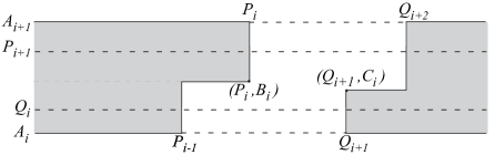
Figure 8. Strip $y\in[A_{i},A_{i+1}]$ of $\Omega_{\bar{A}}$

We will prove the desired properties of the set $\Omega_{\bar{A}}$ stated in Theorem 1.3: property (1) (Theorem 4.2) and property (2) (Theorem 6.1).

Remark 4.1.

Alternatively, the domain of bijectivity of $F_{\bar{A}}$ can be constructed using an approach first described by of I. Smeets in her thesis [10]: start with the known domain $\Omega_{\bar{P}}$ of the Bowen-Series map $F_{\bar{P}}$ and modify it by an infinite “quilting process” by adding and deleting rectangles where the maps $F_{\bar{A}}$ and $F_{\bar{P}}$ differ. In the case of short cycles the “quilting process” gives exactly the region $\Omega_{\bar{A}}$, but unfortunately, it does not work when the cycles are longer. Since in the short cycles case the domain $\Omega_{\bar{A}}$ can be described explicitly, we do not go into the details of the “quilting process” here.

Theorem 4.2.

The map $F_{\bar{A}}:\Omega_{\bar{A}}\rightarrow\Omega_{\bar{A}}$ is one-to-one and onto.

Proof.

We investigate how different regions of $\Omega_{\bar{A}}$ are mapped by $F_{\bar{A}}$. More precisely we look at the strip $S_{i}$ of $\Omega_{\bar{A}}$ given by $y\in[A_{i},A_{i+1}]$, and its image under $F_{\bar{A}}$, in this case $T_{i}$. See Figure 9. We consider the following decomposition of this strip: $\tilde{S}_{i}=[Q_{i+2},P_{i-1}]\times[A_{i},A_{i+1}]$ (red rectangular piece), $S_{i}^{\ell}=[Q_{i+1},Q_{i+2}]\times[A_{i},{C_{i}}]$ (blue lower corner) and $S_{i}^{u}=[P_{i-1},P_{i}]\times[{B_{i}},A_{i+1}]$ (green upper corner). Now

(4.1) $$T_{i}(\tilde{S}_{i}) =T_{i}([Q_{i+2},P_{i-1}]\times[A_{i},A_{i+1}])=[Q_{\sigma(i)},P_{\sigma(i)+1}]\times[B_{\sigma(i)+1},C_{\sigma(i)-1}]$$

(4.2) $$T_{i}(S_{i}^{\ell}) =T_{i}([Q_{i+1},Q_{i+2}]\times[A_{i},{C_{i}}])=[P_{\sigma(i)},Q_{\sigma(i)}]\times[B_{\sigma(i)+1},T_{i}{C_{i}}]$$

(4.3) $$T_{i}(S_{i}^{u}) =T_{i}([P_{i-1},P_{i}]\times[{B_{i}},A_{i+1}])=[P_{\sigma(i)+1},Q_{\sigma(i)+1}]\times[T_{i}{B_{i}},C_{\sigma(i)-1}]$$

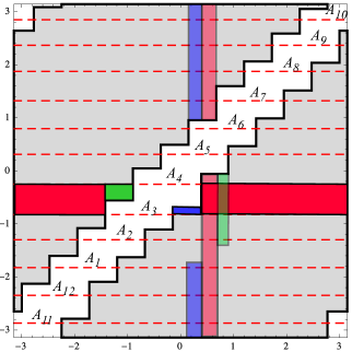
Figure 9. Bijectivity of the $F_{\bar{A}}$ map

Notice that

• $T_{i}(\tilde{S}_{i})$ is a complete vertical strip in $\Omega_{\bar{A}}$, $Q_{\sigma(i)}\leq x\leq P_{\sigma(i)+1}$;

• $T_{i}(S_{i}^{u})$ together with $T_{j}(S_{j}^{\ell})$ (where ${\sigma(j+1)=\sigma(i-1)-1}$) form a complete vertical strip in $\Omega_{\bar{A}}$, $P_{\sigma(i)+1}\leq x\leq Q_{\sigma(i)+1}$. (We are using here the short cycle property $T_{i}T_{\sigma(i-1)}A_{\sigma(i-1)}=T_{j}T_{\sigma(j+1)}A_{\sigma(j+1)+1}$.)

• $T_{i}(S_{i}^{\ell})$ together with $T_{k}(S_{k}^{u})$ (where $\sigma(k)+1=\sigma(i)$) form a complete vertical strip in $\Omega_{\bar{A}}$, $P_{\sigma(i)}\leq x\leq Q_{\sigma(i)}$.

This proves the bijectivity property of $F_{\bar{A}}$ on $\Omega_{\bar{A}}$. ∎

We showed that the ends of the cycles do not appear as $y$-levels of the boundary of $\Omega_{\bar{A}}$. We state this important property as a corollary.

Corollary 4.3.

For $i$ and $j$ related via $\sigma(j+1)=\sigma(i-1)-1$, we have

(4.4) $$T_{j}C_{j}=T_{i}B_{i}\in[B_{\rho(i)+1},C_{\theta(i)}]=[B_{\rho(j)},C_{\theta(j)-1}].$$

5. Trapping region

In order to prove property (2) of $\Omega_{\bar{A}}$, we enlarge it and prove the trapping property for the enlarged region first. Let $\Psi_{\bar{A}}=\Omega_{\bar{A}}\cup\mathcal{D}$, where

$$\mathcal{D}=\bigcup_{i=1}^{8g-4}R_{i}\text{ and }R_{i}=[P_{i-1},P_{i}]\times[Q_{i},B_{i}].$$

Notice that $\Psi_{\bar{A}}$ can be also expressed as $\Psi_{\bar{A}}=\Omega_{\bar{P}}\cup\mathcal{A}$, where $\mathcal{A}=\cup_{i=1}^{8g-4}[Q_{i+1},Q_{i+2}]\times[P_{i},C_{i}]$. The $y$-levels of the upper part of $\Psi_{\bar{A}}$ are given by the $Q_{i}$’s and the $y$-levels of the lower part of $\Psi_{\bar{A}}$ are given by the $C_{i}$’s.

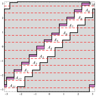
Figure 10. Trapping region $\Psi_{\bar{A}}$ consisting of the set $\Omega_{\bar{A}}$ (grey) and the added set $\mathcal{D}$ (purple)

Theorem 5.1.

The set $\Psi_{\bar{A}}$ is a trapping region for the map $F_{\bar{A}}$, i.e.,

• given any $(x,y)\in{\mathbb{S}}\times{\mathbb{S}}\setminus\Delta$, there exists $n\geq 0$ such that $F_{\bar{A}}^{n}(x,y)\in\Psi_{\bar{A}}$;

• $F_{\bar{A}}(\Psi_{\bar{A}})\subset\Psi_{\bar{A}}$.

Proof.

We start with $(x,y)\in{\mathbb{S}}\times{\mathbb{S}}\setminus\Delta$ and show that there exists $n\geq 0$ such that $F_{\bar{A}}^{n}(x,y)\in\Psi_{\bar{A}}$. We have $Q_{i}\in[A_{i},P_{i+1})\subset[A_{i},A_{i+1})$, and by the short cycle condition, ${C_{i}}\in[A_{i},P_{i+1})\subset[A_{i},A_{i+1})$.

Consider $(x,y)\in{\mathbb{S}}\times{\mathbb{S}}\setminus\Delta$. Notice that there exists $n(x,y)>0$ such that the two values $x_{n},y_{n}$ obtained from the $n$th iterate of $F_{\bar{A}}$, $(x_{n},y_{n})=F^{n}_{\bar{A}}(x,y)$, are not inside the same isometric circle; in other words, $(x_{n},y_{n})\not\in X_{i}=[P_{i},Q_{i+1}]\times[A_{i},A_{i+1})$ for all $1\leq i\leq 8g-4$ (see the argument in the proof of Theorem 2.1).

In order to prove the attracting property we need to analyze the situations $(x_{n},y_{n})\in Y_{i}=[P_{i-1},P_{i}]\times[A_{i},Q_{i})$ (orange set), and $(x_{n},y_{n})\in Z_{i}=[Q_{i+1},Q_{i+2}]\times({C_{i}},A_{i+1}]$ (green set), and show that a forward iterate lands in $\Psi_{\bar{A}}$.

Figure 11. The strip $y\in[A_{i},A_{i+1}]$ of the trapping region $\Psi_{\bar{A}}$ together with the sets $Y_{i}=[P_{i-1},P_{i}]\times[A_{i},Q_{i})$ (orange) and $Z_{i}=[Q_{i+1},Q_{i+2}]\times({C_{i}},A_{i+1}]$ (green) outside of it that require special considerations

Case (I) If $(x_{n},y_{n})\in Y_{i}=[P_{i-1},P_{i}]\times[A_{i},Q_{i})$, then

$$F_{\bar{A}}(x_{n},y_{n})\in[T_{i}P_{i-1},T_{i}P_{i}]\times[T_{i}A_{i},T_{i}Q_{i})=[P_{\rho(i)},Q_{\rho(i)}]\times[B_{\rho(i)},Q_{\rho(i)+1}).$$

Since $B_{\rho(i)}\in[Q_{\rho(i)},A_{\rho(i)+1}]$, we need to analyze the regions

$$[P_{\rho(i)},Q_{\rho(i)}]\times[B_{\rho(i)},A_{\rho(i)+1}]\quad\text{ and }\quad[P_{\rho(i)},Q_{\rho(i)}]\times[A_{\rho(i)+1},Q_{\rho(i)+1}).$$

(a) If $(x_{n+1},y_{n+1})\in[P_{k},Q_{k}]\times[B_{k},A_{k+1}]$, where $k=\rho(i)$, then

$$(x_{n+2},y_{n+2})=T_{k}(x_{n+1},y_{n+1})\in[Q_{\rho(k)},Q_{\rho(k)+1}]\times[T_{k}B_{k},T_{k}A_{k+1}]\,.$$

Since $T_{k}A_{k+1}=C_{\theta(k)}$, and $T_{k}B_{k}\in[B_{\rho(k)+1},C_{\theta(k)}]$ the only part of the vertical strip above where $(x_{n+2},y_{n+2})$ might still lie outside of $\Psi_{\bar{A}}$ is a subset of $[P_{\rho(k)+1},Q_{\rho(k)+1}]\times[B_{\rho(k)+1},Q_{\rho(k)+2})$.

Notice that $\rho(k)=\sigma(\sigma(i)+1)+1=4g+i-2$ (direct verification), so we need to analyze the situation $(x_{n+2},y_{n+2})\in[P_{4g+i-1},Q_{4g+i-1}]\times[B_{4g+i-1},Q_{4g+i})$.

(b) If $(x_{n+1},y_{n+1})\in[P_{k},Q_{k}]\times[A_{k+1},Q_{k+1})$, then

$$(x_{n+2},y_{n+2})=T_{k+1}(x_{n+1},y_{n+1})\in[P_{\rho(k+1)},T_{k+1}Q_{k}]\times[B_{\rho(k+1)},Q_{\rho(k+1)+1})\,.$$

Notice that $T_{k+1}Q_{k}\in[P_{\rho(k+1)},Q_{\rho(k+1)}]$ and $\rho(k+1)=\rho(\rho(i)+1)=i-1$ (direct verification) so we are left to investigate $(x_{n+2},y_{n+2})\in[P_{i-1},Q_{i-1}]\times[B_{i-1},Q_{i})$.

To summarize, we started with $(x_{n+1},y_{n+1})\in[P_{\rho(i)},Q_{\rho(i)}]\times[B_{\rho(i)},Q_{\rho(i)+1})\,$ and found two situations that need to be analyzed $(x_{n+2},y_{n+2})\in[P_{i-1},Q_{i-1}]\times[B_{i-1},Q_{i})$ or $(x_{n+2},y_{n+2})\in[P_{4g+i-1},Q_{4g+i-1}]\times[B_{4g+i-1},Q_{4g+i})$.

We prove in what follows that it is not possible for all future iterates $F^{m}(x_{n},y_{n})$ to belong to the sets of type $[P_{k},Q_{k}]\times[B_{k},Q_{k+1})$.

First, it is not possible for all $F^{m}(x_{n},y_{n})$ (starting with some $m>0$) to belong only to type-a sets $[P_{k_{m}},Q_{k_{m}}]\times[B_{k_{m}},A_{k_{m}+1}]$, where $k_{m+1}=\rho(k_{m})+1$ because such a set is included in the isometric circle $X_{k_{m}}$, and the argument at the beginning of the proof disallows such a situation.

Also, it is not possible for all $F^{m}(x_{n},y_{n})$ (starting with some $m>0$) to belong only to type-b sets $[P_{k_{m}},Q_{k_{m}}]\times[A_{k_{m}+1},Q_{k_{m}+1})$, where $k_{m+1}=\rho(k_{m}+1)$: this would imply that the pairs of points $(y_{n+m},A_{k_{n+m}+1})$ (on the y-axis) will belong to the same interval $[A_{k_{n+m}},Q_{k_{n+m}+1})$ which is impossible due to expansiveness property of the map $f_{\bar{A}}$.

Therefore, there exists a pair $(x_{l},y_{l})$ in the orbit of $F^{m}(x_{n},y_{n})$ such that

$$(x_{l},y_{l})\in[P_{j},Q_{j}]\times[A_{j+1},Q_{j+1})\quad\text{ (type-b)}$$

for some $1\leq j\leq 8g-4$ and

$$(x_{l+1},y_{l+1})\in[P_{j^{\prime}},T_{j+1}Q_{j}]\times[T_{j+1}A_{j+1},P_{j^{\prime}+1}]\subset[P_{j^{\prime}},Q_{j^{\prime}}]\times[Q_{j^{\prime}},P_{j^{\prime}+1}]\quad\text{ (type-a)},$$

where $j^{\prime}=\rho(j+1)$. Then

$$(x_{l+2},y_{l+2})\in T_{j^{\prime}}([P_{j^{\prime}},T_{j+1}Q_{j}]\times[Q_{j^{\prime}},P_{j^{\prime}+1}])=[Q_{j^{\prime\prime}},T_{j^{\prime}}T_{j+1}Q_{j}]\times[Q_{j^{\prime\prime}+1},P_{j^{\prime\prime}-2}]$$

where $j^{\prime\prime}=\rho(j^{\prime})$.

Using the results of the Appendix (Corollary 8.3), we have that the arc length distance satisfies

$$\ell(P_{j^{\prime}},T_{j+1}Q_{j})=\ell(T_{j+1}P_{j},T_{j+1}Q_{j})<\frac{1}{2}\ell(P_{j^{\prime}},Q_{j^{\prime}}).$$

Now we can use Corollary 8.2 (ii) applied to the point $T_{j+1}Q_{j}\in[P_{j^{\prime}},Q_{j^{\prime}}]$ to conclude that $T_{j^{\prime}}T_{j+1}Q_{j}\in[Q_{j^{\prime\prime}},P_{j^{\prime\prime}+1}]$. Therefore $(x_{l+2},y_{l+2})\in\Psi_{\bar{A}}$.

Case (II) If $(x_{n},y_{n})\in Z_{i}=[Q_{i+1},Q_{i+2}]\times(C_{i},A_{i+1}]$, then

$$F_{\bar{A}}(x_{n},y_{n})\in T_{i}([Q_{i+1},Q_{i+2}]\times(C_{i},A_{i+1}])=[P_{\sigma(i)},Q_{\sigma(i)}]\times(T_{i}C_{i},C_{\theta(i)}].$$

Since $T_{i}C_{i}\in[B_{\rho(i)},C_{\theta(i)-1}]$ by (4.4) and the set $[P_{\sigma(i)},Q_{\sigma(i)}]\times[B_{\rho(i)},C_{\theta(i)-1}]$ is in $\Psi_{\bar{A}}$, we are left with analyzing the situation

$$(x_{n+1},y_{n+1})\in[P_{\sigma(i)},Q_{\sigma(i)}]\times(C_{\theta(i)-1},C_{\theta(i)}].$$

This requires two subcases depending on $y_{n+1}\in(C_{k-1},A_{k})$ or $y_{n+1}\in[A_{k},C_{k}]$, where $k=\theta(i)$.

(a) If $(x_{n+1},y_{n+1})\in[P_{k+1},Q_{k+1}]\times(C_{k-1},A_{k})$, then

$$(x_{n+2},y_{n+2})=T_{k-1}(x_{n+1},y_{n+1})\in[T_{k-1}P_{k+1},Q_{\sigma(k-1)}]\times(T_{k-1}C_{k-1},T_{k-1}A_{k}).$$

Notice that $\sigma(k-1)=\sigma(\theta(i)-1)=i+2$ (direct verification). Since

$$T_{k-1}P_{k+1}\in[P_{\sigma(k-1)},Q_{\sigma(k-1)})=[P_{i+2},Q_{i+2}),$$

$T_{k-1}A_{k}=C_{\theta(k-1)}=C_{i+1}$ and $T_{k-1}C_{k-1}\in[B_{\rho(k-1)},C_{\theta(k-1)-1})=[B_{i+3},C_{i})$, we have that $(x_{n+2},y_{n+2})\in[P_{i+2},Q_{i+2})\times[B_{i+3},C_{i+1})$. The only part of this vertical strip where $(x_{n+2},y_{n+2})$ might still lie outside of $\Psi_{\bar{A}}$ is a subset of $[P_{i+2},Q_{i+2}]\times(C_{i},C_{i+1})$, and that is the situation we need to analyze.

(b) If $(x_{n+1},y_{n+1})\in[P_{k+1},Q_{k+1}]\times[A_{k},C_{k}]$, then

$$(x_{n+2},y_{n+2})\in T_{k}\left([P_{k+1},Q_{k+1}]\times[A_{k},C_{k}]\right)=[P_{\sigma(k)-1},P_{\sigma({k})}]\times[B_{\rho(k)},T_{k}C_{k}].$$

Since $T_{k}C_{k}\in[B_{\rho(k)},C_{\theta(k)-1}]$ by (4.4) and $\sigma(k)=\sigma(\theta(i))=4g+i-1$, then

$$(x_{n+2},y_{n+2})\in[P_{4g+i-2},P_{4g+i-1}]\times[B_{4g+i},C_{4g+i-3}]$$

and the only part of this vertical strip where $(x_{n+2},y_{n+2})$ might still lie outside of $\Psi_{\bar{A}}$ is a subset of $[P_{4g+i-2},Q_{4g+i-2}]\times[A_{4g+i-3},C_{4g+i-3}]$.

To summarize, we started with $(x_{n+1},y_{n+1})\in[P_{\sigma(i)},Q_{\sigma(i)}]\times(C_{\theta(i)-1},C_{\theta(i)}]$ and found two situations that need to be analyzed $(x_{n+2},y_{n+2})\in[P_{i+2},Q_{i+2}]\times(C_{i},C_{i+1}]$ or $(x_{n+2},y_{n+2})\in[P_{4g+i-2},Q_{4g+i-2}]\times[A_{4g+i-3},C_{4g+i-3}]$.

We prove that it is not possible for all future iterates $F^{m}(x_{n},y_{n})$ to belong to the sets of type $[P_{k+1},Q_{k+1}]\times[C_{k-1},C_{k}]$.

First, it is not possible for all $F^{m}(x_{n},y_{n})$ (starting with some $m>0$) to belong only to type-a sets $[P_{k_{m}+1},Q_{k_{m}+1}]\times(C_{k_{m}-1},A_{k_{m}})$, where $k_{m+1}=\sigma(k_{m}-1)$: this would imply that the pairs of points $(y_{n+m},A_{k_{n+m}})$ (on the $y$-axis) will belong to the same interval $(C_{k_{n+m}-1},A_{k_{n+m}}]\subset[A_{k_{n+m}-1},A_{k_{n+m}}]$ which is impossible due to expansiveness property of the map $f_{\bar{A}}$ on such intervals.

From the discussion of Case (b), if an iterate $F^{m}(x_{n},y_{n})$ belongs to a type-b set, then $F^{m+1}(x_{n},y_{n})$ either belongs to $\Psi_{\bar{A}}$ or to another type-b set. However, it is not possible for all iterates $F^{m}(x_{n},y_{n})$ (starting with some $m>0$) to belong to type-b sets $[P_{k_{m}+1},Q_{k_{m}+1}]\times[A_{k_{m}},C_{k_{m}}]$, where $k_{m+1}=\sigma(k_{m})-2$ because such a set is included in the isometric circle $X_{k_{m}}$, and the argument at the beginning of the proof disallows such a situation. Thus, once an iterate $F^{m}(x_{n},y_{n})$ belongs to a type-b set, then it will eventually belong to $\Psi_{\bar{A}}$.

We showed that any point $(x,y)$ that belongs to a set $[P_{k+1},Q_{k+1}]\times(C_{k-1},C_{k}]$ will have a future iterate in $\Psi_{\bar{A}}$. This completes the proof of Case II and, hence, the theorem. ∎

6. Reduction theory

We can now complete the proof of Theorem 1.3.

Theorem 6.1.

For almost every point $(x,y)\in{\mathbb{S}}\times{\mathbb{S}}\setminus\Delta$, there exists $K>0$ such that $F_{\bar{A}}^{K}(x,y)\in\Omega_{\bar{A}}$, and the set $\Omega_{A}$ is a global attractor for $F_{\bar{A}}$, i.e.,

$$\Omega_{A}=\bigcap_{n=0}^{\infty}F_{\bar{A}}^{n}({\mathbb{S}}\times{\mathbb{S}}\setminus\Delta).$$

Proof.

By Theorem 5.1, every point $(x,y)\in{\mathbb{S}}\times{\mathbb{S}}\setminus\Delta$ is mapped to the trapping region $\Psi_{\bar{A}}=\Omega_{\bar{A}}\cup\mathcal{D}$ by some iterate $F_{\bar{A}}^{n}$. Therefore, it suffices to track the set $\mathcal{D}=\bigcup_{i=1}^{8g-4}R_{i}$. The image of each rectangle $R_{i}=[P_{i-1},P_{i}]\times[Q_{i},B_{i}]$ under $F_{\bar{A}}$, $F_{\bar{A}}(R_{i})=T_{i}(R_{i})$, is a rectangular set

(6.1) $$F_{\bar{A}}(R_{i})=[T_{i}P_{i-1},T_{i}P_{i}]\times[T_{i}Q_{i},T_{i}B_{i}]=[P_{\rho(i)},Q_{\rho(i)}]\times[Q_{\rho(i)+1},T_{i}B_{i}].$$

The “top” of this rectangle, $[P_{\rho(i)},Q_{\rho(i)}]\times\{T_{i}B_{i}\}$ is inside $\Omega_{\bar{A}}$, since $T_{i}B_{i}\in[B_{\rho(i)+1},C_{\theta(i)}]$. Moreover,

(6.2) $$F_{\bar{A}}(R_{i})\setminus\Omega_{\bar{A}}=[P_{\rho(i)},Q_{\rho(i)}]\times[Q_{\rho(i)+1},B_{\rho(i)+1}]\subset R_{\rho(i)+1},$$

so, by letting $j=\rho(i)+1$,

$$F_{\bar{A}}(\mathcal{D})\setminus\Omega_{\bar{A}}=\bigcup_{j=1}^{8g-4}[P_{j-1},Q_{j-1}]\times[Q_{j},B_{j}]$$

and

$$F_{\bar{A}}(\Omega_{\bar{A}}\cup\mathcal{D})=\Omega_{\bar{A}}\cup\bigcup_{j=1}^{8g-4}[P_{j-1},Q_{j-1}]\times[Q_{j},B_{j}].$$

Now the image of the rectangular set $[P_{j-1},Q_{j-1}]\times[Q_{j},B_{j}]$ under $F_{\bar{A}}(=T_{j})$ is

$$F_{\bar{A}}([P_{j-1},Q_{j-1}]\times[Q_{j},B_{j}])=[P_{\rho(j)},T_{j}Q_{j-1}]\times[Q_{\rho(j)+1},T_{j}B_{j}],$$

hence

(6.3) $$F_{\bar{A}}\big{(}F_{\bar{A}}(\mathcal{D}))\setminus\Omega_{\bar{A}}=\bigcup_{j=1}^{8g-4}[P_{\rho(j)},T_{j}Q_{j-1}]\times[Q_{\rho(j)+1},B_{\rho(j)+1}].$$

Corollary 8.3 tells us that the length of the segment $[P_{\rho(j)},T_{j}Q_{j-1}]=T_{j}([P_{j-1},Q_{j-1}])$ is less than $\frac{1}{2}$ of $[P_{\rho(j)},Q_{\rho(j)}]$. If we let $k=\rho(j)+1$, and denote $T_{j}Q_{j-1}$ by $S^{(2)}_{k}$, then (6.3) becomes

$$F^{2}_{\bar{A}}(\mathcal{D})\setminus\Omega_{\bar{A}}=\bigcup_{k=1}^{8g-4}[P_{k-1},S^{(2)}_{k-1}]\times[Q_{k},B_{k}]$$

with the length of the segment $[P_{k-1},S^{(2)}_{k-1}]$ being less than $\frac{1}{2}$ of $[P_{k-1},Q_{k-1}]$. Inductively, it follows that:

(6.4) $$F^{n}_{\bar{A}}(\mathcal{D})\setminus\Omega_{\bar{A}}=\bigcup_{k=1}^{8g-4}[P_{k-1},S^{(n)}_{k-1}]\times[Q_{k},B_{k}]$$

where the length of the segment $[P_{k-1},S^{(n)}_{k-1}]$ is less than $\frac{1}{2^{n-1}}$ of $[P_{k-1},Q_{k-1}]$. Thus,

$$F^{n}_{\bar{A}}(\Omega_{\bar{A}}\cup\mathcal{D})=\Omega_{\bar{A}}\cup\bigcup_{k=1}^{8g-4}[P_{k-1},S^{(n)}_{k-1}]\times[Q_{k},B_{k}]$$

and

$$\bigcap_{n=0}^{\infty}F_{\bar{A}}^{n}({\mathbb{S}}\times{\mathbb{S}}\setminus\Delta) =\bigcap_{n=0}^{\infty}F_{\bar{A}}^{n}(\Omega_{A}\cup\mathcal{D})=\Omega_{\bar{A}}\cup\bigcap_{n=0}^{\infty}\left(\bigcup_{k=1}^{8g-4}[P_{k-1},S^{n}_{k-1}]\times[Q_{k},B_{k}]\right)$$

$$=\Omega_{\bar{A}}\cup\bigcup_{k=1}^{8g-4}\{P_{k-1}\}\times[Q_{k},B_{k}]=\Omega_{\bar{A}}$$

In what follows, we will show that any point $(x,y)\in\mathcal{D}$ (see Figure 10) is actually mapped to $\Omega_{\bar{A}}$ after finitely many iterations with the exception of the Lebesgue measure zero set consisting of the union of horizontal segments $\bigcup_{i=1}^{8g-4}[P_{i-1},P_{i}]\times\{Q_{i}\}$ and their preimages. For that, let $(x,y)\in R_{i}$ with $y\neq Q_{i}$ and assume that $F_{\bar{A}}^{n}(x,y)=(x_{n},y_{n})\in F^{n}_{\bar{A}}(\mathcal{D})\setminus\Omega_{\bar{A}}$. Using (6.4), this means that the sequence of points $y_{n}\in(Q_{k_{n}},B_{k_{n}}]$ for all $n\geq 1$. But $y_{n+1}=T_{k_{n}}y_{n}$, $Q_{k_{n}+1}=T_{k_{n}}Q_{k_{n}}$ and the map $T_{k_{n}}$ is (uniformly) expanding on $[Q_{k_{n}},B_{k_{n}}]$ (a subset of the isometric circle of $T_{k_{n}}$), which contradicts the assumption $y_{n}\in(Q_{k_{n}},B_{k_{n}}]$. ∎

7. Invariant measures

It is a standard computation that the measure $d\nu=\displaystyle\frac{|dx|\,|dy|}{|x-y|^{2}}$ is preserved by Möbius transformations applied to unit circle variables $x$ and $y$, hence by $F_{\bar{A}}$. Therefore, $F_{\bar{A}}$ preserves the smooth probability measure

(7.1) $$d\nu_{\bar{A}}=\frac{1}{K_{\bar{A}}}d\nu,\text{ where }K_{\bar{A}}=\int_{\Omega_{\bar{A}}}d\nu.$$

Alternatively, by considering $F_{\bar{A}}$ as a reduction map acting on geodesics, the invariant measure can be derived more elegantly by using the geodesic flow on the hyperbolic disk and the Poincaré cross-section maps, but we are not pursuing that direction here.

In what follows, we compute $K_{\bar{A}}$ for the case when $\bar{A}$ satisfies the short cycle property. Recall that the domain $\Omega_{\bar{A}}$ was described in the proof of Theorem 4.2 as:

(7.2) $$\Omega_{\bar{A}}=\bigcup_{i=1}^{8g-4}[Q_{i+2},P_{i-1}]\times[A_{i},A_{i}+1]\cup[Q_{i+1},Q_{i+2}]\times[A_{i},C_{i}]\cup[P_{i-1},P_{i}]\times[B_{i},A_{i+1}].$$

Proposition 7.1.

If the points $A_{i}$ satisfy the short cycle property and $p_{i},q_{i},b_{i},c_{i}$ represent the angular coordinates of $P_{i}$, $Q_{i}$, $B_{i}=T_{i}A_{i}$, and $C_{i}=T_{i-1}A_{i}$, respectively, then

(7.3) $$\nu(\Omega_{A})=K_{A}=\ln\prod_{i=1}^{8g-4}\frac{|\sin\left(\frac{c_{i}-q_{i+2}}{2}\right)||\sin\left(\frac{b_{i}-p_{i-1}}{2}\right)|}{|\sin\left(\frac{b_{i}-p_{i}}{2}\right)||\sin\left(\frac{c_{i}-q_{i+1}}{2}\right)|}.$$

Proof.

Since $\Omega_{A}$ is given by (7.2), we have

$$K_{\bar{A}}=\int_{\Omega_{\bar{A}}}d\nu=\sum_{i=1}^{8g-4}\left(\int_{Q_{i+2}}^{P_{i-1}}\int_{A_{i}}^{A_{i+1}}d\nu+\int_{Q_{i+1}}^{Q_{i+2}}\int_{A_{i}}^{C_{i}}d\nu+\int_{P_{i-1}}^{P_{i}}\int_{B_{i}}^{A_{i+1}}d\nu\right).$$

In order to compute each of the three integrals above, we use angular coordinates $\theta$ and $\phi$ corresponding to $x=e^{i\theta}$, $y=e^{i\phi}$, and write for some arbitrary values $A,B,C,D$:

$$I_{A,B,C,D}:=\displaystyle\int_{A}^{B}\int_{C}^{D}\frac{|dx||dy|}{|x-y|^{2}} =\displaystyle\int_{a}^{b}\int_{c}^{d}\frac{d\theta d\phi}{|\exp(i\theta)-\exp(i\phi)|^{2}}$$

$$=\int_{a}^{b}\int_{c}^{d}\frac{d\theta d\phi}{2-2\cos(\theta-\phi)}=:I_{a,b,c,d},$$

where $a,b,c,d$ are the angular coordinates corresponding to $A,B,C,D$:

$$A=e^{ia},B=e^{ib},C=e^{ic},D=e^{id}.$$

The double integral (which we denoted by $I_{a,b,c,d}$) can be computed explicitly. First

(7.4) $$\int_{a}^{b}\frac{d\theta}{2-2\cos(\theta-\phi)}=-\frac{1}{2}\cot\left(\frac{\theta-\phi}{2}\right)\biggr{|}_{\theta=a}^{\theta=b}=\frac{1}{2}\left(\cot\left(\frac{a-\phi}{2}\right)-\cot\left(\frac{b-\phi}{2}\right)\right).$$

Then, using the fact that the antiderivative $\int\cot xdx=\ln|\sin x|$ we obtain

$$I_{a,b,c,d} =\frac{1}{2}\int_{c}^{d}\left(\cot\left(\frac{a-\phi}{2}\right)-\cot\left(\frac{b-\phi}{2}\right)\right)d\phi$$

$$=\left(\ln\left|\sin\left(\frac{\phi-b}{2}\right)\right|-\ln\left|\sin\left(\frac{\phi-a}{2}\right)\right|\right)\biggr{|}_{\phi=c}^{\phi=d}$$

$$=\ln\left|\sin\left(\frac{d-b}{2}\right)\right|+\ln\left|\sin\left(\frac{c-a}{2}\right)\right|-\ln\left|\sin\left(\frac{c-b}{2}\right)\right|-\ln\left|\sin\left(\frac{d-a}{2}\right)\right|$$

$$=\ln\frac{|\sin\left(\frac{d-b}{2}\right)||\sin\left(\frac{c-a}{2}\right)|}{|\sin\left(\frac{c-b}{2}\right)||\sin\left(\frac{d-a}{2}\right)|}.$$

Now, using the angular coordinates $p_{i},q_{i},a_{i},b_{i},c_{i}$ corresponding to the points $P_{i}$, $Q_{i}$, $A_{i}$, $B_{i}$, $C_{i}$, we obtain

$$K_{\bar{A}} =\sum_{i=1}^{8g-4}(I_{q_{i+2},p_{i-1},a_{i},a_{i+1}}+I_{q_{i+1}q_{i+2},a_{i},c_{i}}+I_{p_{i-1},p_{i},b_{i},a_{i+1}})$$

$$=\ln\prod_{i=1}^{8g-4}\frac{|\sin\left(\frac{a_{i+1}-p_{i-1}}{2}\right)||\sin\left(\frac{a_{i}-q_{i+2}}{2}\right)|}{|\sin\left(\frac{a_{i}-p_{i-1}}{2}\right)||\sin\left(\frac{a_{i+1}-q_{i+2}}{2}\right)|}+\ln\prod_{i=1}^{8g-4}\frac{|\sin\left(\frac{c_{i}-q_{i+2}}{2}\right)||\sin\left(\frac{a_{i}-q_{i+1}}{2}\right)|}{|\sin\left(\frac{a_{i}-q_{i+2}}{2}\right)||\sin\left(\frac{c_{i}-q_{i+1}}{2}\right)|}$$

$$\quad+\ln\prod_{i=1}^{8g-4}\frac{|\sin\left(\frac{a_{i+1}-p_{i}}{2}\right)||\sin\left(\frac{b_{i}-p_{i-1}}{2}\right)|}{|\sin\left(\frac{b_{i}-p_{i}}{2}\right)||\sin\left(\frac{a_{i+1}-p_{i-1}}{2}\right)|}$$

$$=\ln\prod_{i=1}^{8g-4}\frac{|\sin\left(\frac{c_{i}-q_{i+2}}{2}\right)||\sin\left(\frac{b_{i}-p_{i-1}}{2}\right)|}{|\sin\left(\frac{b_{i}-p_{i}}{2}\right)||\sin\left(\frac{c_{i}-q_{i+1}}{2}\right)|}.$$

The last equality is obtained due to cancellations. ∎

The circle map $f_{\bar{A}}$ is a factor of $F_{\bar{A}}$ (projecting on the $y$-coordinate), so one can obtain its smooth invariant probability measure $d\mu_{\bar{A}}$ by integrating $d\nu_{\bar{A}}$ over $\Omega_{\bar{A}}$ with respect to the $u$-coordinate. Thus, from the exact shape of the set $\Omega_{\bar{A}}$, we can calculate the invariant measure precisely.

Proposition 7.2.

$\displaystyle d\mu_{\bar{A}}=\frac{1}{K_{\bar{A}}}\sum_{i=1}^{8g-4}\left(\cot\left(\frac{q_{i+1}-\phi}{2}\right)-\cot\left(\frac{p_{i}-\phi}{2}\right)\right)d\phi.$

Proof.

$$d\mu_{\bar{A}}=\frac{1}{K_{\bar{A}}}\sum_{i=1}^{8g-4}\left(\int_{Q_{i+2}}^{P_{i-1}}\frac{|dx|}{|x-y|^{2}}+\int_{Q_{i+1}}^{Q_{i+2}}\frac{|dx|}{|x-y|^{2}}+\int_{P_{i-1}}^{P_{i}}\frac{|dx|}{|x-y|^{2}}\right)|dy|.$$

Using the calculations (7.4) we obtain

$$d\mu_{\bar{A}} =\frac{1}{K_{\bar{A}}}\sum_{i=1}^{8g-4}\Bigg{(}\cot\left(\frac{q_{i+2}-\phi}{2}\right)-\cot\left(\frac{p_{i-1}-\phi}{2}\right)$$

$$\qquad\qquad\quad+\cot\left(\frac{q_{i+1}-\phi}{2}\right)-\cot\left(\frac{q_{i+2}-\phi}{2}\right)$$

$$\qquad\qquad\quad+\cot\left(\frac{p_{i-1}-\phi}{2}\right)-\cot\left(\frac{p_{i}-\phi}{2}\right)\Bigg{)}d\phi$$

$$=\frac{1}{K_{\bar{A}}}\sum_{i=1}^{8g-4}\left(\cot\left(\frac{q_{i+1}-\phi}{2}\right)-\cot\left(\frac{p_{i}-\phi}{2}\right)\right)d\phi.\qed$$

8. Appendix

In this section we use the explicit description of the fundamental domain $\mathcal{F}$ given in the Introduction to obtain certain estimates used in the proofs.

The fundamental domain $\mathcal{F}$ is a regular $(8g-4)$-gon bounded by the isometric circles of the generating transformations of $\Gamma$ with all internal angles equal to $\frac{\pi}{2}$. Let us label the vertices of $\mathcal{F}$ by $V_{1},\dots,V_{8g-4}$, where $V_{i}$ is the intersection of the geodesics $P_{i-1}Q_{i}$ and $P_{i}Q_{i+1}$ (see Figure 12 for $g=3$). We first prove the following geometric lemma.

Lemma 8.1.

Consider five consecutive isometric circles of $\mathcal{F}$: $P_{i-2}Q_{i-1}$, $P_{i-1}Q_{i}$, $P_{i}Q_{i+1}$, $P_{i+1}Q_{i+2}$, and $P_{i+2}Q_{i+3}$. Then

1. the angle between geodesics $V_{i+1}P_{i+2}$ and $V_{i+1}Q_{i+1}$ is greater than $\frac{\pi}{4}$,

2. the angle between geodesics $V_{i}Q_{i-1}$ and $V_{i}P_{i}$ is greater than $\frac{\pi}{4}$.

Proof.

Let the Euclidean distance from the center of the unit disk $\mathbb{D}$, $O$, to the center of each isometric circle be $d$, the Euclidean radius of each isometric circle by $R$, and $v$ be the distance from $O$ to the vertex $V_{i+1}$ (see Figure 12). The angle between the imaginary axis and the ray from the origin to $V_{i+1}$ is equal to $t=\frac{\pi}{8g-4}$. The angle between geodesics $V_{i+1}P_{i+2}$ and $V_{i+1}Q_{i+1}$ is equal to the angle between the radii of the Euclidean circles (of centers $O_{i}$, $O^{\prime}_{i+1}$) representing these geodesics, i.e., $\angle O_{i}V_{i+1}O^{\prime}_{i+1}$. Our goal is to express it as a function of $t$, $\omega(t)$.

Let $\varphi=\angle O_{i}OQ_{i+1}$. We have $\sin\varphi=|O_{i}Q_{i+1}|/d$, and $\sin t=|O_{i}H|/d$, where $O_{i}H\perp OH$. Since the angle of $\mathcal{F}$ at $V_{i+1}$ is equal to $\frac{\pi}{2}$, $|O_{i}H|=|O_{i}V_{i+1}|/\sqrt{2}$, and since $|O_{i}V_{i+1}|=|O_{i}Q_{i+1}|=R$, we obtain

(8.1) $$\sin\varphi=\sqrt{2}\sin t,$$

and therefore

(8.2) $$\cos\varphi=\sqrt{\cos(2t)}.$$

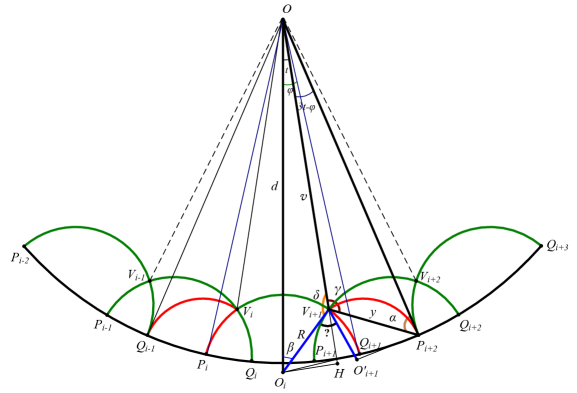
Figure 12. Calculation of angle $\angle O_{i}V_{i+1}O^{\prime}_{i+1}$

In the right triangle $\Delta O_{i}OH$ we have $|OH|=v+\frac{R}{\sqrt{2}}$ and $|O_{i}H|=\frac{R}{\sqrt{2}}$, hence by the Pythagorean Theorem,

$$\left(v+\frac{R}{\sqrt{2}}\right)^{2}+\frac{R^{2}}{2}=d^{2}=\frac{R^{2}}{2\sin^{2}t},$$

which implies

$$v+\frac{R}{\sqrt{2}}=\frac{R}{\sqrt{2}}\cot t,$$

and hence

$$v=\frac{R}{\sqrt{2}}\left(\frac{\cos t}{\sin t}-1\right).$$

Using that $R=\sqrt{2}\sin(t)d$ and $d=\displaystyle\frac{1}{\cos\varphi}=\frac{1}{\sqrt{\cos(2t)}}$, we obtain $R$ and $v$ as functions of $t$,

(8.3) $$R(t)=\frac{\sqrt{2}\sin t}{\sqrt{\cos(2t)}},\quad v(t)=\sqrt{\frac{\cos t-\sin t}{\cos t+\sin t}},$$

and we now can express all further quantities as functions of $t$.

In the triangle $\Delta OO_{i}V_{i+1}$, let $\angle OO_{i}V_{i+1}=\beta(t)$ and $\angle OV_{i+1}O_{i}=\delta(t)$. In the triangle $\Delta OP_{i+2}V_{i+1}$, let $|V_{i+1}P_{i+2}|=y(t)$, $\angle OP_{i+2}V_{i+1}=\alpha(t)$, $\angle OV_{i+1}P_{i+2}=\gamma(t)$. One can easily see that $\angle V_{i+1}OP_{i+2}=3t-\varphi(t)$. Using the Rule of Cosines, we have

$$y(t)^{2}=1+v(t)^{2}-2v(t)\cos(3t-\varphi).$$

Using the Rule of Sines in the triangles $\Delta OP_{i+2}V_{i+1}$ and $\Delta OO_{i}V_{i+1}$ we obtain

$$\sin(\alpha(t))=\frac{v(t)\sin(3t-\varphi)}{y(t)},\quad\sin(\beta(t))=\frac{v(t)\sin(t)}{R(t)}=\frac{\cos t-\sin t}{\sqrt{2}},$$

and the last equation implies $\beta=\frac{\pi}{4}-t$.

The angle $\omega(t)=\angle O_{i}V_{i+1}O^{\prime}_{i+1}$ in question is calculated as

$$\omega(t)=2\pi-\gamma(t)-\delta(t)-\left(\frac{\pi}{2}-\alpha(t)\right).$$

Expressing $\gamma(t)$ and $\delta(t)$ from these triangles we obtain

(8.4) $$\omega(t) =4t-\varphi(t)+2\alpha(t)+\beta(t)-\frac{\pi}{2}$$

$$=4t-\varphi(t)+2\alpha(t)+\frac{\pi}{4}-t-\frac{\pi}{2}$$

$$=3t-\varphi(t)+2\alpha(t)-\frac{\pi}{4}.$$

We see that the desired inequality

(8.5) $$\omega(t)>\frac{\pi}{4}$$

is equivalent to $3t-\varphi(t)+2\alpha(t)>\frac{\pi}{2}$, and since from $\Delta OV_{i+1}P_{i+2}$ we have

$$3t-\varphi(t)+\alpha(t)+\gamma(t)=\pi,$$

(8.5) is equivalent to

(8.6) $$\gamma(t)-\alpha(t)<\frac{\pi}{2}.$$

Recall that $\gamma(t)$ and $\alpha(t)$ are the angles of the triangle $\Delta OV_{i+1}P_{i+2}$, with $\gamma(t)>\frac{\pi}{2}$ and $\alpha(t)<\frac{\pi}{2}$, hence $0<\gamma(t)-\alpha(t)<\pi$. In order to prove (8.6), we need to show that

(8.7) $$\cos(\gamma(t)-\alpha(t))>0.$$

Using the Rule of Sines we obtain

$$\sin\gamma(t)=\frac{\sin\alpha(t)}{v(t)}.$$

Using the Rule of Cosines we obtain

$$\cos\gamma(t)=\frac{y^{2}(t)+v^{2}(t)-1}{2y(t)v(t)}\text{ and }\cos\alpha=\frac{1+y^{2}(t)-v^{2}(t)}{2y(t)}.$$

In what follows we will suppress dependence of all functions on $t$. Thus

$$\cos(\gamma-\alpha) =\cos\gamma\cos\alpha+\sin\gamma\sin\alpha$$

$$=\frac{(y^{2}+v^{2}-1)(1+y^{2}-v^{2})}{4y^{2}v}+\frac{\sin^{2}\alpha}{v}$$

$$=\frac{8v^{2}-4v(1+v^{2})\cos(3t-\varphi)}{4vy^{2}}.$$

Since $v$ and $y$ are positive, it is sufficient to prove the positivity of the function

$$g(t) =\frac{2v}{(1+v^{2})}-\cos(3t-\varphi)=\frac{\cos\varphi}{\cos t}-\cos(3t-\varphi)$$

$$=\frac{\cos\varphi}{\cos t}-\cos((3t-2\varphi)+\varphi)$$

$$=\frac{\cos\varphi}{\cos t}-(\cos(3t-2\varphi)\cos\varphi-\sin(3t-2\varphi)\sin\varphi)$$

$$=\cos\varphi\left(\frac{1}{\cos t}-\cos(3t-2\varphi)\right)+\sin(3t-2\varphi)\sin\varphi.$$

The first term is positive since $\cos\varphi$, $\cos t$ and $\cos(3t-2\varphi)$ are less than $1$. The second term is positive since

(8.8) $$3t-2\varphi>0.$$

The latter follows from the fact that the function

$$h(t)=3t-2\varphi(t)=3t-2\arcsin(\sqrt{2}\sin t)$$

has second derivative

$$h^{\prime\prime}(t)=-\frac{2\sqrt{2}\sin t}{\cos^{3/2}(2t)}$$

negative on $(0,\pi/12]$, hence

$$h^{\prime}(t)=3-\frac{2\sqrt{2}\cos t}{\cos^{1/2}(2t)}$$

is decreasing on $(0,\pi/12]$, so $h^{\prime}(t)\geq h^{\prime}(\pi/12)=3-\displaystyle\frac{\sqrt{2}+\sqrt{6}}{{3}^{1/4}}>0$ for any $t\in(0,\pi/12]$. Thus, $h$ is strictly increasing on $(0,\pi/12]$, so $h(t)>h(0)=0$ for any $t\in(0,\pi/12]$ which implies (8.8). Thus (8.5) follows. The second inequality follows from the symmetry of the fundamental domain $\mathcal{F}$. ∎

In what follows $\ell$ will denote the arc length on the unit circle ${\mathbb{S}}$.

Corollary 8.2.

1. There exist $a_{j},b_{j}\in(P_{j},Q_{j})$ such that $d(P_{j},a_{j})>\frac{1}{2}\ell(P_{j},Q_{j})$ and $\ell(b_{j},Q_{j})>\frac{1}{2}\ell(P_{j},Q_{j})$ such that $T_{j}(a_{j})=P_{\rho(j)+1}$ and $T_{j-1}(b_{j})=Q_{\theta(j-1)}$.

2. For any point $x\in[P_{j},Q_{j}]$ such that $\ell(P_{j},x)\leq\frac{1}{2}\ell(P_{j},Q_{j})$, we have $T_{j}(x)\in[Q_{\sigma(j)+1},P_{\sigma(j)+2}]$.

3. For any point $x\in[P_{j},Q_{j}]$ such that $\ell(x,Q_{j})\leq\frac{1}{2}\ell(P_{j},Q_{j})$, we have $T_{j-1}(x)\in[Q_{\theta(j-1)},P_{\theta(j-1)+1}]$.

Proof.

(i) Let $M_{j}$ be the midpoint of $[P_{j},Q_{j}]$. Since the angle at each $V_{j}$ is equal to $\frac{\pi}{2}$, the angle between the geodesic segments $V_{j}P_{j}$ and $V_{j}M_{j}$ is equal $\frac{\pi}{4}$. Recall that $T_{j}([P_{j},Q_{j}])=[Q_{\rho(j)},Q_{\rho(j)+1}]$. Since, by Lemma 8.1 (i) for $i=\sigma(j)$, the angle between the geodesic segments $V_{\rho(j)}P_{\rho(j)+1}$ and $V_{\rho(j)}Q_{\rho(j)}$ is $>\frac{\pi}{4}$, and $T_{j}$ is conformal, the existence of $a_{j}\in(M_{j},Q_{j})$ such that $T_{j}(a_{j})=P_{\rho(j)+1}$ follows. Similarly, we know that $T_{j-1}([P_{j},Q_{j}])=[P_{\theta(j-1)},P_{\theta(j-1)+1}]$. Since by Lemma 8.1 (ii) with $i=\sigma(j-1)$, the angle between the geodesic segments $V_{\sigma(j-1)}Q_{\theta(j-1)}$ and $V_{\sigma(j-1)}P_{\theta(j-1)+1}$ is greater than $\frac{\pi}{4}$ and $T_{j-1}$ is conformal, the existence of $b_{j}\in(P_{j},M_{j})$ such that $T_{j-1}(b_{j})=Q_{\theta(j-1)}$ follows. Parts (ii) and (iii) follow immediately from (i). ∎

Corollary 8.3.

The arc length of the interval $T_{k}([P_{k+2},Q_{k+2}])$ is less than $\frac{1}{2}$ of $[P_{\sigma(k)},Q_{\sigma(k)}]$ and the length of the interval $T_{k}([P_{k-1},Q_{k-1}])$ is less than $\frac{1}{2}$ of $[P_{\sigma(k)+1},Q_{\sigma(k)+1}]$.

Proof.

By Proposition 2.2, we have $T_{k}(Q_{k+1})=P_{\sigma(k)}$ and $T_{k}(Q_{k+2})=Q_{\sigma(k)}$. The fact that the length of $T_{k}([P_{k+2},Q_{k+2}])<\frac{1}{2}\ell(P_{\sigma(k)},Q_{\sigma(k)})$ is equivalent to the fact that $T_{k}(P_{k+2})\in[M_{\sigma(k)},Q_{\sigma(k)}]$, where $M_{\sigma(k)}$ is the middle of $[P_{\sigma(k)},Q_{\sigma(k)}]$. But the last statement follows from the fact that the angle between the geodesic $V_{k+1}P_{k+2}$ and the geodesic $V_{k+1}Q_{k+2}$ is less then $\frac{\pi}{4}$, a direct consequence of the fact that the angle in the part (i) of Lemma 8.1 is greater that $\frac{\pi}{4}$. The second statement follows immediately from the part (ii) of Lemma 8.1. ∎

Acknowledgments. We thank the anonymous referee for several useful comments and suggestions.

References

- [1] R. Adler, L. Flatto, Geodesic flows, interval maps, and symbolic dynamics, Bull. Amer. Math. Soc. 25 (1991), no. 2, 229–334.
- [2] W. Ambrose, S. Kakutani, Structure and continuity of measurable flows, Duke Math. J., 9 (1942), 25–42.
- [3] R. Bowen, C. Series, Markov maps associated with Fuchsian groups, Inst. Hautes Études Sci. Publ. Math. No. 50 (1979), 153–170.
- [4] G.A. Jones, D. Singerman, Complex Functions, Cambridge University Press, 1987
- [5] S. Katok, Fuchsian Groups, University of Chicago Press, 1992.
- [6] S. Katok, I. Ugarcovici, Structure of attractors for -continued fraction transformations, Journal of Modern Dynamics, 4 (2010), 637–691.
- [7] S. Katok, I. Ugarcovici, Applications of -continued fraction transformations, ETDS (2012).
- [8] B. Maskit, On Poincaré s Theorem for fundamental polygons, Adv. Math., 7 (1971), 219–230.
- [9] C. Series, Symbolic dynamics for geodesic flows, Acta Math. 146 (1981), 103–128.
- [10] I. Smeets, On continued fraction algorithms, PhD thesis, Leiden, 2010.
- [11] D. Zagier, Possible notions of “good” reduction algorithms, personal communication, 2007.