Rigorous Results in Existence and Selection of Saffman-Taylor Fingers by Kinetic Undercooling

Abstract.

The selection of Saffman-Taylor fingers by surface tension has been extensively investigated. In this paper we are concerned with the existence and selection of steadily translating symmetric finger solutions in a Hele-Shaw cell by small but non-zero kinetic undercooling ($\epsilon^{2}$). We rigorously conclude that for relative finger width $\lambda$ near one half, symmetric finger solutions exist in the asymptotic limit of undercooling $\epsilon^{2}~{}\rightarrow~{}0$ if the Stokes multiplier for a relatively simple nonlinear differential equation is zero. This Stokes multiplier $S$ depends on the parameter $\alpha\equiv\frac{2\lambda-1}{(1-\lambda)}\epsilon^{-\frac{4}{3}}$ and earlier calculations have shown this to be zero for a discrete set of values of $\alpha$. While this result is similar to that obtained previously for Saffman-Taylor fingers by surface tension, the analysis for the problem with kinetic undercooling exhibits a number of subtleties as pointed out by Chapman and King (2003) [The selection of Saffman-Taylor fingers by kinetic undercooling, Journal of Engineering Mathematics 46, 1-32]. The main subtlety is the behavior of the Stokes lines at the finger tip, where the analysis is complicated by non-analyticity of coefficients in the governing equation.

Keywords: finger selection, Hele-Shaw, kinetic undercooling, existence, analytic solution

1. Introduction

1.1. Background

The problem of a less viscous fluid displacing a more viscous fluid in a Hele-Shaw cell has been the subject of numerous studies since the 1950s. In a seminal paper, Saffman & Taylor [28] found experimentally that an unstable planar interface evolves through finger competition to a steady translating finger, with relative finger width $\lambda$ close to one half. Theoretical calculations [40], [28] ignoring surface tension revealed an one-parameter family of exact steady solutions, parameterized by width $\lambda$. When the experimentally determined $\lambda$ is used, the theoretical shape (usually referred to in the literature as the Saffman-Taylor finger) agreed well with experiments for relatively large displacement rates, or equivalently for small surface tension. However, in the zero-surface-tension steady-state theory, $\lambda$ remained undetermined in the (0, 1) interval. The selection of $\lambda$ remained unresolved until the mid 1980s. Numerical calculations [21], [37], [18], supported by formal asymptotic calculations in the steady finger [6], [30], [17], [32], [4] and the closely-related steady Hele-Shaw bubble problem [9, 31], suggest that a discrete family of solutions exist for which the limiting shape, as surface tension tends to zero, approaches the Saffman-Taylor finger with $\lambda=\frac{1}{2}$. Rigorous results were later obtained in [38, 35].

The Hele-Shaw problem is similar to the Stefan problem in the context of melting or freezing. Besides surface tension, the physical effect most commonly incorporated in regularizing the ill-posed Stefan problem is kinetic undercooling [14, 19, 2], where the temperature on the moving interface is proportional to the normal velocity of the interface. The Stefan problem also arises in some other physical situations such as the diffusion of solvent through glassy polymers [7, 20] and the interfacial approximation of the streamer stage in the evolution of sparks and lightning [13].

For the Hele-Shaw problem, kinetic undercooling regularization first appeared in [26, 27]. Local existence of analytic solution was obtained in [24, 25] for the time dependent Hele-Shaw problem with kinetic undercooling. Using exponential asymptotics, Chapman and King [5] analyzed the selection problem of determining the discrete set of widths of a traveling finger for varying kinetic undercooling. Some numerical studies have been attempted in [12, 15]. A continuum of corner-free traveling fingers were obtained numerically in [12] for any finger width above a critical value, while a discrete set of analytic fingers, as predicted in [5], were computed in [15]. The physical connection between the kinetic undercooling effect and the action of the dynamic contact angle was established in [1].

The aims of this paper are to establish some rigorous results in existence and selection of symmetric analytic solutions to the Hele-Shaw problem with sufficiently small kinetic undercooling.

1.2. Mathematical Formulation

We consider the problem of a finger of inviscid fluid displacing a viscous fluid in a Hele-Shaw cell for small kinetic undercooling (Fig.1).

Figure 1. A translating finger in the Hele-Shaw cell

The gap-averaged velocity $(u,v)$ in the $(x,y)$ plane in the region outside the finger satisfies

(1.1) $$(u,v)=-\frac{b^{2}}{12\mu}\nabla p\equiv\nabla\phi,$$

where $b$ is the gap width, $\mu$ the viscosity of the viscous fluid and $p$ denotes the pressure. Incompressibility of fluid flow implies zero divergence of fluid velocity, implying that the velocity potential $\phi$ satisfies

(1.2) $$\Delta\phi=0~{}~{}~{}{\rm for}~{}~{}(x,y)\in\Omega.$$

The boundary conditions on the side walls are

(1.3) $$v=0~{}~{}{\rm when}~{}~{}y=\pm{a}.$$

The far field condition is

(1.4) $$(u,v)=V{\hat{x}}+O(1)\text{ as }x\to+\infty,$$

where ${\hat{x}}$ is a unit vector in the $x$-direction (along the Hele-Shaw channel) and $V$ is the constant displacement rate of the fluid far away. The kinematic condition for a steady finger is

(1.5) $$\frac{\partial\phi}{\partial n}=U\cos\theta,$$

where $\theta$ is the angle between the interface normal and the positive x -axis (see Fig. 1) and $U$ is the speed of the finger. The kinetic undercooling condition

(1.6) $$\phi=cv_{n}=cU\cos\theta,$$

where $c>0$ is the kinetic undercooling parameter. There are a number of different but equivalent formulations [21, 32, 5, 34], here we use the formulation which parallels that in Tanveer [34]. We set the channel half-width $a=1$ and displacement rate $V=1$, which corresponds to non-dimensionalizing all lengths by $a$ and velocities by $V$ (consequently time is measured in units of $a/V$).

By integrating (1.2) in the domain $\Omega$, the finger width $\lambda$ is related to $U$ as follows:

(1.7) $$\lambda=\frac{1}{U}.$$

In a frame moving with the steady symmetric finger, the condition (1.5) transforms, without loss of generality, into

(1.8) $$\psi=0,$$

where $\psi$ is the stream function ( the harmonic conjugate of $\phi$ ) so that $W=\phi+i\psi$ is an analytic function of $z=x+iy$. The nondimensional kinetic undercooling condition (1.6) in the moving frame becomes

(1.9) $$\phi+\frac{1}{\lambda}x=\frac{c}{\lambda}\cos\theta.$$

On the side walls, (1.3) implies that

(1.10) $$\psi=\pm\left[\frac{1}{\lambda}-1\right]\text{ on }y=-1\text{ and }y=1\text{ respectively}$$

while the far field condition as $z~{}\rightarrow~{}+\infty$ in the finger frame is

(1.11) $$W\sim-\left[\frac{1}{\lambda}-1\right]z+O(1).$$

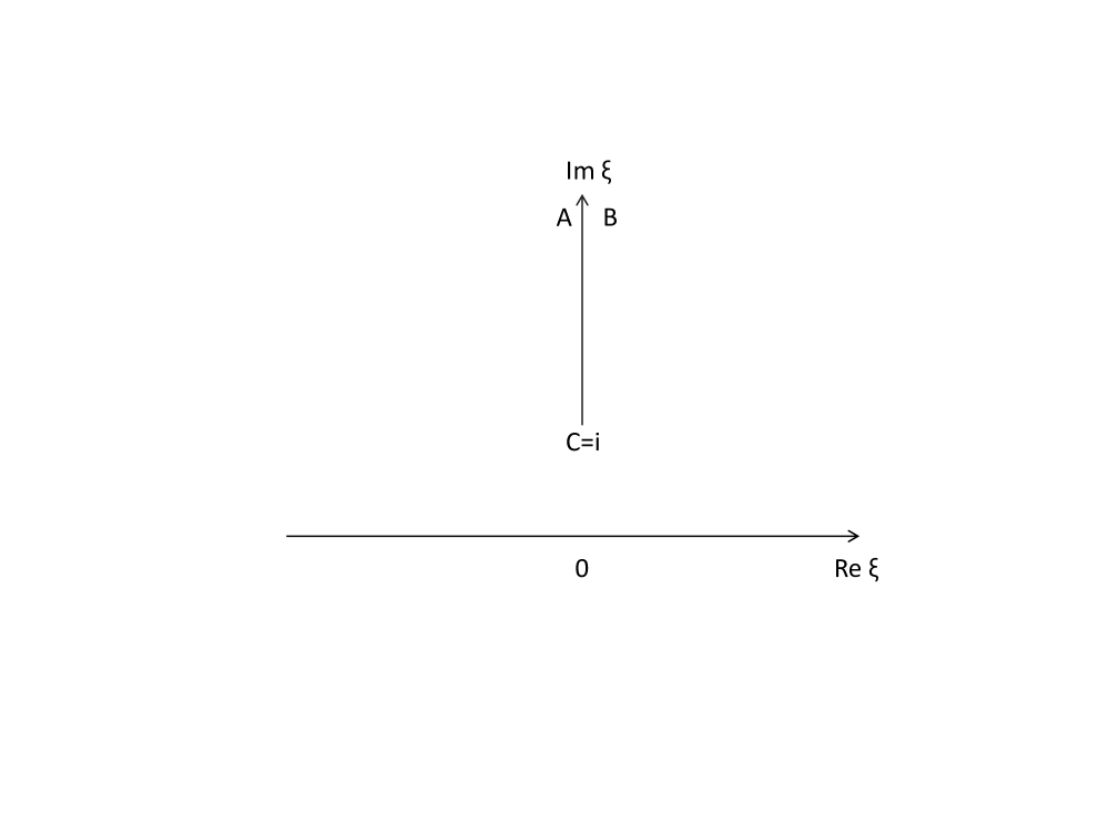
Figure 2. Upper half $\xi$-plane with a cut on the imaginary axis from $\xi=i$ to $i\infty$

We consider the conformal map $z(\xi)$ of the cut upper-half-$\xi$-plane, as shown in Figure 2, to the flow domain $\Omega$ in Figure 1. The real $\xi$ axis corresponds to the finger boundary, with $\xi=-\infty,+\infty$ corresponding to the finger tails at $z=-\infty+\lambda i,z=-\infty-\lambda i$ respectively. The two sides of the cut correspond to the two side walls respectively. It is easily seen that the complex potential $W(\xi)$ is given by:

(1.12) $$W(\xi)=\frac{1-\lambda}{\pi\lambda}\ln~{}(\xi^{2}+1)+constant.$$

We define $F(\xi)$ so that

(1.13) $$z(\xi)=-\frac{1}{\pi}\ln~{}(\xi-i)-\frac{1-2\lambda}{\pi}\ln~{}(\xi+i)-\lambda i-\frac{2-2\lambda}{\pi}F(\xi).$$

It follows that $F$, as defined above, is analytic in the entire upper half $\xi$-plane [34]. The kinetic undercooling condition (1.9) translates into requiring that on the real $\xi$ axis:

(1.14) $$\text{Re }F=-\epsilon^{2}\frac{\text{Im }(F^{\prime}+H)}{|F^{\prime}+H|},$$

where

(1.15) $$H(\xi)=\frac{\xi+\gamma i}{\xi^{2}+1},\quad\text{ with }\gamma=\frac{\lambda}{1-\lambda},~{}\epsilon^{2}=\frac{c\pi}{2\lambda(1-\lambda)}.$$

For zero kinetic undercooling $\epsilon=0$, it follows that $F=0$; this corresponds to what is usually referred to in the literature as the Saffman-Taylor solutions [40, 28]. This form a family of exact solutions for symmetric fingers with arbitrary width of finger $\lambda\in(0,~{}1)$ . The Saffman-Taylor solutions, in our formulation, correspond to the conformal map

(1.16) $$z_{0}(\xi)=-\frac{1}{\pi}\ln~{}(\xi-i)-\frac{1-2\lambda}{\pi}\ln~{}(\xi+i)-\lambda i.$$

This is easily seen to be univalent since the boundary correspondence is one to one. In particular, the finger shape can be explicitly described by Re $z$ as a function of Im $z$.

For non-zero kinetic undercooling, no exact solutions exist. Numerical and asymptotic work [5, 12, 15] suggested that solutions exist for infinitely many isolated values of finger width which are larger than $\frac{1}{2}$. The aim of this paper is to obtain rigorous results for this selection problem, in particular the existence of a symmetric and analytic solution for sufficient small undercooling constant $c$.

1.3. Notations

Definition 1.1.

Let $\mathcal{R}$ be an open connected (see Figure 3) region on complex $\xi$ plane bounded by lines $r_{u}$ and $r_{l}$ defined as follows:

$$r_{u}=r_{u,1}\cup r_{u,2}\cup r_{u,3}\cup r_{u,4}\cup r_{u,5}\cup r_{u,6}$$

$$r_{l}=\{\xi:\xi=-bi+re^{-i(\varphi_{0}+\mu)}\}\cup\{\xi:\xi=-bi+re^{i(\pi+\varphi_{0}+\mu)}\}$$

where $0<b<\min~{}(1,\gamma)$, $~{}0<\varphi_{0},~{}\mu~{}<~{}\frac{\pi}{2}$ with $\varphi_{0}+\mu<\frac{\pi}{2}$ and

$$r_{u,1}=\{\xi:\xi=\nu_{1}i-R+re^{i(\pi-\varphi_{0})},0\leq r<\infty\}~{},~{}$$

$$r_{u,2}=\{\xi:\text{ Im }\xi=\nu_{1},-R\leq\text{Re }\xi\leq-\nu_{1}\},$$

$$r_{u,3}=\{\xi:\xi=re^{3\pi i/4},0\leq r\leq\sqrt{2}\nu_{1}\},~{}$$

$$r_{u,4}=\{\xi:\xi=re^{\pi i/4}\},0\leq r\leq\sqrt{2}\nu_{1}\},$$

$$r_{u,5}=\{\xi:\text{ Im }\xi=\nu_{1},\nu_{1}\leq\text{ Re }\xi\leq R\}~{},~{}$$

$$r_{u,6}=\{\xi:\xi=\nu_{1}i+R+re^{i\varphi_{0}},0\leq r<\infty\},$$

where $R>0$ is large enough and $0<\nu_{1}$ is small enough so that Lemma 6.3 - Lemma 6.8 in the appendix hold.

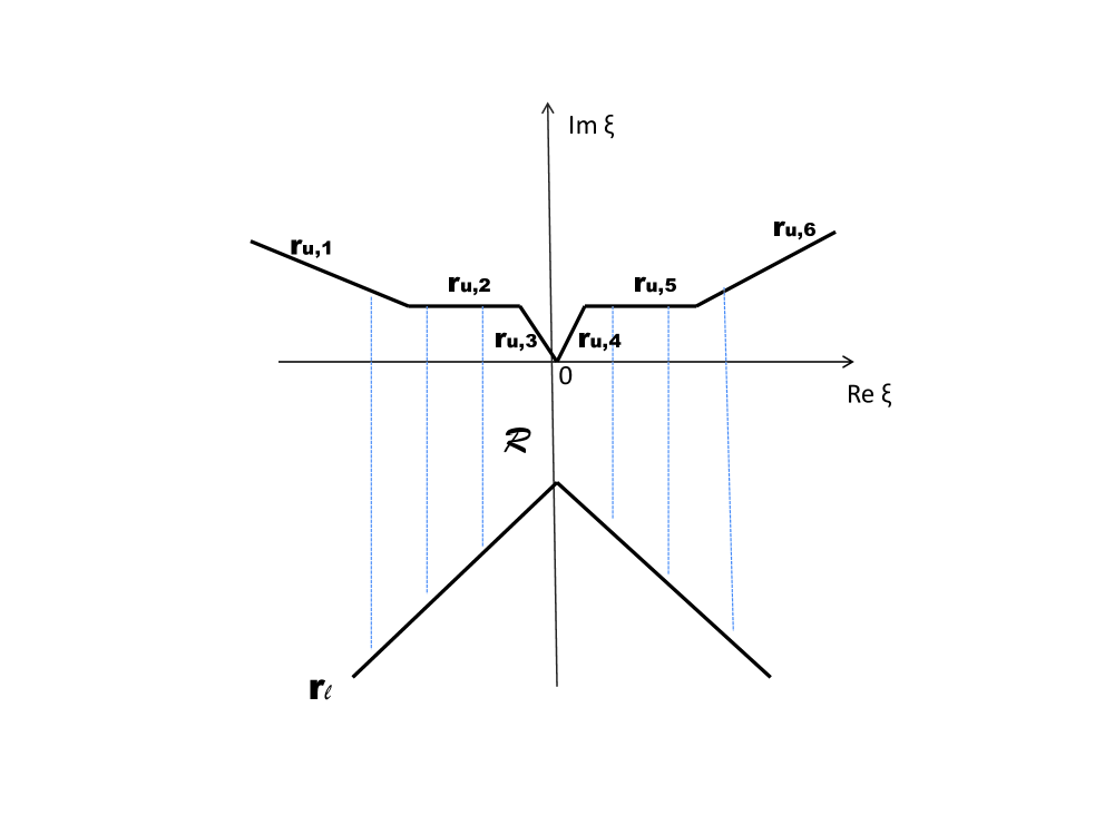
Figure 3. Region $\mathcal{R}$ in the complex $\xi$ plane given in Definition 1.1

Remark 1.2.

$1-b$, and $\varphi_{0}$ are chosen independently of $\epsilon$. There are some restrictions imposed on their values in order that certain lemmas in the appendix are ensured.

Definition 1.3.

$\mathcal{R}^{-}=\mathcal{R}\cap\{\text{ Re }\xi~{}<~{}0\}~{};~{}\mathcal{R}^{+}=\mathcal{R}\cap\{\text{ Re }\xi~{}>~{}0\}$

Let $0<\tau<1$ be independent of $\epsilon$, $\nu>0$ be a small number, and $B_{\nu}=\{\xi:|\xi|<\nu\}$. We introduce spaces of functions:

Definition 1.4.

Define

$$\begin{split}\mathbf{A}^{-}_{0}&=\{F:F(\xi)~{}\text{analytic in }\mathcal{R}^{-}\text{~{}and continuous in }\overline{\mathcal{R}^{-}},\\ &~{}~{}~{}\text{ with }\underset{\xi\in\overline{\mathcal{R}^{-}}}{\sup}~{}\left|(\xi-2i)^{\tau}F(\xi)\right|<\infty\\ &~{}~{}~{}\text{and }\underset{\xi\in\overline{\mathcal{R}^{-}}}{\sup}~{}\left|\frac{F^{\prime}(\xi)-F^{\prime}(0)}{\sqrt{\xi}}\right|<\infty\}\end{split}$$

$$\lVert F\rVert_{0}^{-}:=\underset{\xi\in\overline{\mathcal{R}^{-}}}{\sup}~{}\lvert(\xi-2i)^{\tau}F(\xi)\rvert+\epsilon^{2}\underset{\xi\in\overline{\mathcal{R}^{-}\cap B_{\nu}}}{\sup}~{}\left|\frac{F^{\prime}(\xi)-F^{\prime}(0)}{\sqrt{\xi}}\right|+|F^{\prime}(0)|.$$

Remark 1.5.

$\mathbf{A}^{-}_{0}$ is a Banach space. If $F\in\mathbf{A}_{0}^{-}$, then $F$ satisfies property:

(1.17) $$F(\xi)\sim O(\xi^{-\tau}),~{}\text{ as }|\xi|\to\infty,~{}\xi\in\mathcal{R}^{-}.$$

In Definition 1.4, replacing $\mathcal{R}^{-}$ with $\mathcal{R}$ we can define $\mathbf{A}\equiv\mathbf{A}_{0}$ with norm

$$\lVert F\rVert_{0}:=\underset{\xi\in\overline{\mathcal{R}}}{\sup}~{}\lvert(\xi-2i)^{\tau}F(\xi)\rvert+\epsilon^{2}\underset{\xi\in\overline{\mathcal{R}\cap B_{\nu}}}{\sup}~{}\left|\frac{F^{\prime}(\xi)-F^{\prime}(0)}{\sqrt{\xi}}\right|+|F^{\prime}(0)|.$$

Remark 1.6.

Locally in a neighborhood of $\xi=0$, $\mathbf{A}_{0}$ contains functions which are analytic at $\xi=0$, it also contains functions $F(\xi)$ which are NOT analytic at $\xi=0$ such as $F(\xi)=C\xi^{k+3/2},k=0,1,2,\cdots$ with a branch cut on upper half plane. If $F(\xi)\in\mathbf{A}_{0}$ is analytic in the upper half plane, then $F(\xi)$ has to be analytic at $\xi=0$.

Definition 1.7.

Let $\mathcal{D}$ be any connected set in the complex $\xi$-plane; we introduce norms: $\lVert F\rVert_{k,\mathcal{D}}:=\underset{\xi\in\mathcal{D}}{\sup}~{}\lvert(\xi-2i)^{k+\tau}F(\xi)\rvert,\quad k=0,1,2$.

Definition 1.8.

Let $\delta>0$ be a constant, define space:

$$\mathbf{A}^{-}_{0,\delta}=\{f:f\in\mathbf{A}_{0}^{-},~{}\lVert f\rVert^{-}_{0}\leq\delta\}.$$

$\mathbf{A}_{0,\delta}$ can be defined similarly.

Remark 1.9.

For $\lambda$ in a compact subset of (0, 1) and for sufficiently small enough $\delta$, if $F\in\mathbf{A}_{0,\delta}$, then the mapping $z(\xi)$ given by (1.13) is univalent. See Theorem 1.5 in [38].

The problem of determining a smooth steady symmetric finger is equivalent to finding function $F$ analytic in the upper-half $\xi$ plane, which is $\mathbf{C^{1}}$ in its closure, i.e. continuous derivative on Im $\xi=0$ and is required to satisfy the following conditions:
Condition (i): $F(\xi)$ satisfies (1.14) on the real $\xi$ axis.

Condition (ii):

(1.18) $$F(\xi)\to 0\quad\text{ as }\xi\to\pm\infty.$$

Condition (iii) ( symmetry condition ):

(1.19) $$\text{Re }F(-\xi)=\text{Re }F(\xi)~{},~{}\text{Im }F(-\xi)=-\text{Im }F(\xi)\quad\text{for }~{}\xi~{}\text{real}.$$

Remark 1.10.

If $F\in\mathbf{A}_{0}$ is analytic in the upper half plane, and satisfies symmetry condition (iii) on the real axis, then it follows from successive Taylor expansions of $F(\xi)$ on the imaginary $\xi$ axis segment $-b~{}<~{}\text{Im }\xi$, starting at $\xi=0$ that Im $F(\xi)=0$. From the Schwartz reflection principle, $F(\xi)=\left[F(-\xi^{*})\right]^{*}$, so $\lVert F\rVert_{0}^{-}=\lVert F\rVert^{+}_{0}$. Conversely, if $F\in\mathbf{A}_{0}^{-}$ and satisfies Im $F(\xi)=0$ for the imaginary $\xi$ axis segment $-b~{}<~{}\text{Im }\xi~{}<~{}0$, then $F(\xi)=\left[F(-\xi^{*})\right]^{*}$ extends $F$ to the right half of $\mathcal{R}$ and $\lVert F\rVert_{0}^{-}=\lVert F\rVert_{0}$ and (1.19) is then automatically satisfied.

Finger problem: The problem tackled in this paper will be to find function $F$ analytic in $\{\text{Im }\xi>0\}\cup\mathcal{R}$ so that $F\in\mathbf{A}_{0,\delta}$ for some $\tau$ fixed in (0, 1), $\delta$ small, so that conditions (i) and (iii) on the real axis are satisfied.

1.4. Main Results

Similar to the finger problem with surface tension [6, 8, 32, 38], the formal strategy of calculation of finger width involves analytic continuation of equation in an inner neighborhood of turning points in the complex plane and ignoring integral contribution and other terms that are formally small. As in Chapman and King [5], the problem of determining a smooth steady finger is reduced to determining eigenvalues $\alpha$ so that $G(y)$ is a solution to

(1.20) $$\frac{dG}{dy}-\frac{1}{yG^{2}}=-y-\frac{\alpha}{2^{1/3}y}$$

satisfying the condition

(1.21) $$yG(y)\to 1\quad\text{ as }y\to\infty\text{ and }\arg y\in[0,\pi/4),$$

and in addition satisfying:

(1.22) $$\text{Im }G=0,\text{ for large enough $y$ on the positive real axis.}$$

The finger width $\lambda$ is related to $\alpha$ through

(1.23) $$\alpha=\frac{2\lambda-1}{1-\lambda}\epsilon^{-4/3}.$$

We introduce additional change in variables:

(1.24) $$\eta=\frac{2}{3}y^{3}~{},~{}\psi(\eta)=1-yG(y),$$

then (1.20) becomes:

(1.25) $$\frac{d\psi}{d\eta}+\psi=-\frac{1}{3\eta}-\frac{1}{3\eta}\psi+\frac{\alpha}{6^{2/3}\eta^{2/3}}+\frac{1}{2}\sum_{n=2}^{\infty}(-1)^{n}(n+1)\psi^{n}$$

and matching condition:

(1.26) $$\lim_{\eta\to\infty,~{}\arg\eta\in\left(0,\frac{3\pi}{4}\right)}\psi(\eta,\alpha)=0.$$

One of the theorems proved in this paper is

Theorem 1.11.

(1) There exists sufficiently large enough $\rho_{0}>0$ such that (1.25) with condition (1.26) has unique analytic solution $\psi_{0}(\eta,\alpha)$ in the region $|\eta|>\rho_{0},~{}\arg\eta\in[0,\frac{3\pi}{4}]$.
(2) Further on the real $\eta$ axis as $\eta\to\infty$

(1.27) $$\mathrm{Im}~{}\psi_{0}(\eta,\alpha)\sim\tilde{S}(\alpha)e^{-\eta}.$$

(3) Also $\mathrm{Im}~{}\psi_{0}(\eta,\alpha)=0$ for real $\eta$ and $\eta>\rho_{0}$ if and only if $\tilde{S}(\alpha)=0$.

We will not compute the Stokes constants $\tilde{S}(\alpha)$ in this paper, Chapman and King’s numerical computation [5] indicates that there exist a discrete set $\{\alpha_{n}\}$ so that $\tilde{S}(\alpha_{n})=0,\tilde{S}^{\prime}(\alpha_{n})\neq 0$. It is to be noted that the theory of exponential asymptotics for general nonlinear ordinary differential equations [11] makes it possible to rigorously confirm these calculations to within small error bounds. This analysis will be carried out for this problem in a future work.

The primary result of this paper for the finger problem is the following:

Theorem 1.12.

In a range $\frac{1}{2}\leq\lambda\leq\lambda_{m}$, $\delta$ and $\lambda_{m}-\frac{1}{2}$ small (but independent of $\epsilon$) so that (2.24) holds, the following statement hold for all sufficiently small $\epsilon$:
For each $\beta_{0}$ for which the Stokes constant $\tilde{S}(\beta_{0})=0$ in Theorem 1.11, if ${\tilde{S}}^{\prime}(\beta_{0})~{}\neq~{}0$, there exists an analytic function $\beta(\epsilon^{2/3})$ with $\lim_{\epsilon\to 0}\beta(\epsilon^{2/3})=\beta_{0}$ so that if

(1.28) $$\frac{2\lambda-1}{1-\lambda}=\epsilon^{4/3}\beta(\epsilon^{2/3}),$$

then there exists a solution of the Finger problem $F\in\mathbf{A}_{0,\delta}$. Hence for small $\epsilon$,

(1.29) $$\frac{2\lambda-1}{1-\lambda}=\epsilon^{4/3}\left(\beta_{0}+\beta_{1}\epsilon^{2/3}+\beta_{2}\epsilon^{4/3}+\cdots\right).$$

The proof of this theorem is given at the end of §4, after many preliminary results. Our solution strategy consists of two steps:

(a) Relaxing the symmetry condition $F(\xi)=[F(-\xi^{*})]^{*}$ on the imaginary axis interval $-b<\text{Im }\xi<0$, (i.e. Im $F=0$ is relaxed on that Im $\xi$-axis segment), we prove the existence of solutions to an appropriate problem in the half strip $\mathcal{R}^{-}$ for any $\lambda$ belonging to a compact subset of $(0,1)$, for all sufficiently small $\epsilon$. There is no restriction on $\lambda$ otherwise.

(b) The symmetry condition is then invoked to determine a restriction on $\lambda$ that will guarantee existence of solution to the Finger problem. In this part, we restrict our analysis to $\lambda\in[\frac{1}{2},\lambda_{m}]$.

In Section 2, we prove equivalence of the finger problem to a set of two problems (Problem 1 and Problem 2) in a complex strip domain. Problem 1 is to solve an integro-differential equation for $F$ in a Banach space $\mathbf{A}_{0}$. By deforming the contour of integration for the integral term in Problem 1, we obtain Problem 2. By relaxing symmetry condition on an Im $\xi$ axis segment, we derive the Half Problem in the left half strip $\mathcal{R}^{-}$.

In Section 3, by constructing a normal sequence, we prove the existence of solutions to the Half Problem for $\lambda$ in a compact subset of (0, 1) for all sufficiently small $\epsilon$. In Section 4, we carry out step (b) in our solution strategy. By introducing suitably scaled dependent and independent variables in a neighborhood of a turning point, we formulate the inner problem. For the leading order inner-equation, the form of exponentially small terms are obtained and Theorem 1.11 is proved. For the full problem, using the implicit function theorem, it is argued that for small $\epsilon$, and $\beta_{0}$ so that $\tilde{S}(\beta_{0})=0$ and $\tilde{S}^{\prime}(\beta_{0})\neq 0$, there exists a analytic functions $\beta(\epsilon^{2/3})$ so that if $\alpha=\beta(\epsilon^{2/3})$, then Im $F=0$ on $\{\text{ Re }\xi=0\}\cap\mathcal{R}$. This implies that symmetry condition (1.19) is satisfied; hence Theorem 1.12 follows.

While the main result and strategy of proof are similar to that in [38] for Saffman-Taylor fingers by surface tension, the analysis for the problem with kinetic undercooling exhibits a number of subtleties as pointed out by Chapman and King [5]. The main subtlety is the behavior of Stokes lines at the finger tip, where the analysis is complicated by non-analyticity of a coefficient in equation (3.10) in section 3.

2. Formulation of Equivalent Problems

In this particular section, we are going to formulate Problem 1 and Problem 2 which will be proved to be equivalent to the Finger Problem defined in Section 1. We then formulate a half problem in terms of an integro-differential equation in $\mathcal{R}^{-}$, but relax the symmetry condition Im $F=0$ on the imaginary $\xi$-axis segment $(-bi,0)$, which follows from (1.19) (see Remark 1.10). Problem 2, unlike Problem 1, involves nonlocal quantities ($I_{2}$ for instance) with integration paths outside domain $\mathcal{R}$. Hence, when symmetry is relaxed for $F$ in the half problem, singularities at the origin from nonlocal contributions can be estimated conveniently in terms of $F$ from the domain $\mathcal{R}^{-}$ . In this section, as well as the next, we will restrict $\lambda$ to a compact subset of (0, 1) so that all the constants appearing in all estimates are independent of $\lambda$.

2.1. Formulation of Problem 1

Definition 2.1.

Define

(2.1) $$\bar{H}(\xi)=[H(\xi^{*})]^{*}=\frac{\xi-\gamma i}{\xi^{2}+1},$$

(2.2) $$\bar{F}(\xi)=[F(\xi^{*})]^{*}.$$

Remark 2.2.

If $F$ is analytic in domain $\mathcal{D}$ containing the real axis with property (1.17), then $\bar{F}$ is analytic in $\mathcal{D^{*}}$ and $\bar{F}(\xi)=F^{*}(\xi)$ for $\xi$ real and $\bar{F}(\xi)\sim O(\xi^{-\tau})$, as $|\xi|\to\infty,\xi\in\mathcal{D^{*}}$;   $\bar{F^{\prime}}(\xi)\sim O(\xi^{-1-\tau})$, $\bar{F^{\prime\prime}}(\xi)\sim O(\xi^{-2-\tau})$ as $|\xi|\to\infty,\xi\in\mathcal{D^{\prime*}}$, where $\mathcal{D^{\prime}}$ is any angular subset of $\mathcal{D}$ and superscript ^∗ denotes conjugate domain obtained by reflecting about the real axis.

Definition 2.3.

Let $\mathcal{D}$ be a connected set; for any two functions $f,g$ with derivative existing in $\mathcal{D}$ and small enough $\lVert f^{\prime}\rVert_{1,\mathcal{D}}$ and $\lVert g^{\prime}\rVert_{1,\mathcal{D}}$ so that $f^{\prime}+H\neq 0,g^{\prime}+\bar{H}\neq 0$ in $\mathcal{D}$, we define operator $G$ so that

(2.3) $$G(f,g)[t]:=\frac{1}{(f^{\prime}(t)+H(t))^{1/2}(g^{\prime}(t)+\bar{H}(t))^{1/2}}\times\left[(f^{\prime}(t)+H(t))-(g^{\prime}(t)+\bar{H}(t))\right].$$

Remark 2.4.

If $F\in\mathbf{A}$ and $F^{\prime}+H\neq 0$ in $\mathcal{R}$, then $G(F,\bar{F})(t)$ is analytic in $\mathcal{R}\cap\mathcal{R}^{*}$, since in that case $\bar{F}^{\prime}+\bar{H}\neq 0$ in $\mathcal{R}^{*}$.

Lemma 2.5.

Let $\mathcal{D}$ and $f,g$ be as in definition 2.3. If each of dist $(\mathcal{D},-i)$, dist $(\mathcal{D},i)~{}$, dist $(\mathcal{D},-\gamma i)$, and dist $(\mathcal{D},\gamma i)$ are greater than 0 and independent of $\epsilon$, as $\epsilon\to 0$, then we have for small enough $\lVert f^{\prime}\rVert_{1,\mathcal{D}},\lVert g^{\prime}\rVert_{1,\mathcal{D}}$,

(2.4) $$\lVert G(f,g)\rVert_{0,\mathcal{D}}\leq\frac{C(1+\lVert g^{\prime}\rVert_{1,\mathcal{D}}+\lVert f^{\prime}\rVert_{1,\mathcal{D}})}{(K_{1}-\lVert f^{\prime}\rVert_{1,\mathcal{D}})(K_{1}-\lVert g^{\prime}\rVert_{1,\mathcal{D}})},$$

where

(2.5) $$\begin{split}0<H_{m}&\leq\underset{\mathcal{D}}{\inf}~{}\{|(t-2i)H(t)|,|(t-2i)\bar{H}(t)|\},\\ K&\geq\underset{\mathcal{D}}{\sup}~{}|t-2i|^{-\tau}>0,\\ K_{1}&=\frac{H_{m}}{K}>0.\end{split}$$

Constants $C$, $K$ and $K_{1}$ are independent of $\epsilon$ and $\lambda$, since $\lambda$ is in a compact subset of $(0,1)$.

Proof.

Without ambiguity, the norms $\lVert\cdot\rVert$ denoted in this proof refer to $\lVert\cdot\rVert_{.,\mathcal{D}}$, where $\sup$ is over the domain $\mathcal{D}$.

Using (1.15), (2.1):

$$\sup\{|t-2i|^{2}|\bar{H}(t)-H(t)|\}\leq C,$$

$$\sup|(t-2i)H|\leq C,~{}\sup|(t-2i)\bar{H}|\leq C,$$

where $C$ is made independent of $\epsilon$ and $\lambda$ for $\lambda$ in a fixed compact subset of (0, 1). We also have

(2.6) $$\begin{split}|(f^{\prime}(t)+H(t))|&\geq\left[H_{m}|t-2i|^{-1}-\lVert f^{\prime}\rVert_{1}|t-2i|^{-1-\tau}\right]\\ &\geq(H_{m}-K\lVert f^{\prime}\rVert_{1})|t-2i|^{-1}\\ &\geq C(K_{1}-\lVert f^{\prime}\rVert_{1})|t-2i|^{-1},\\ |(g^{\prime}(t)+\bar{H}(t))|&\geq\left[H_{m}|t-2i|^{-1}-\lVert g^{\prime}\rVert_{1}|t-2i|^{-1-\tau}\right]\\ &\geq(H_{m}-K\lVert g^{\prime}\rVert_{1})|t-2i|^{-1}\\ &\geq C(K_{1}-\lVert g^{\prime}\rVert_{1})|t-2i|^{-1},\end{split}$$

where $C$ is made independent of $\epsilon$ and $\lambda$. (2.4) follows immediately from (2.6) . ∎

Lemma 2.6.

If $F\in\mathbf{A}$, then $G(F,\bar{F})(t)=O(t^{-\tau}),$ as $|t|\to\infty,t$ in any angular subdomain of $\mathcal{R}\cap\mathcal{R}^{*}$.

Proof.

From Remark 1.5, Remark 2.2 and Lemma 2.5, with $\mathcal{D}$ being an angular subdomain of $\mathcal{R}\cap\mathcal{R^{*}}$, the proof follows. ∎

Remark 2.7.

Let $H_{m},K,K_{1}$ be as in (2.5) of Lemma 2.5 with $\mathcal{D}$ being an angular subdomain of $\mathcal{R}\cap\mathcal{R^{*}}$, then $H_{m},K,K_{1}$ can be chosen to be independent of $\epsilon$ and $\lambda$ since $\lambda$ is in a fixed compact subset of (0, 1). If $\lVert F^{\prime}\rVert_{1,\mathcal{D}}<\frac{K_{1}}{2}$ then,

(2.7) $$|\xi-2i||F^{\prime}+H|\geq(H_{m}-|\xi-2i|^{-\tau}\lVert F^{\prime}\rVert_{1})\geq C(K_{1}-\lVert F^{\prime}\rVert_{1})>C\frac{K_{1}}{2}>0;$$

so $F^{\prime}+H\neq 0$ holds in $\mathcal{D}$.

Remark 2.8.

Let $\lVert F^{\prime}\rVert_{1,\mathcal{D}}<\frac{K_{1}}{2}$ , by Remark 2.7, we have $\bar{F}^{\prime}+\bar{H}\neq 0$ in $\mathcal{R}^{*}$, so $G(F,\bar{F})$ is analytic in $\mathcal{D}$ which is an angular subdomain of $\mathcal{R}\cap\mathcal{R}^{*}$.

Definition 2.9.

Let $F\in\mathbf{A}$,$\lVert F^{\prime}\rVert_{1,\mathcal{D}}<\frac{K_{1}}{2}$, $\mathcal{D}$ is an angular subdomain of $\mathcal{R}\cap\mathcal{R}^{*}$ and $(-\infty,\infty)\subset\mathcal{D}$, define operator $I$ so that

(2.8) $$I(F)[\xi]=-\frac{1}{2\pi}\int_{-\infty}^{\infty}\frac{G(F,\bar{F})(t)dt}{t-\xi}\quad\text{ for Im }\xi~{}<~{}0.$$

Lemma 2.10.

Let $F\in\mathbf{A}$ be analytic in $\mathrm{Im}~{}\xi>0$ as well. If $F(\xi)$ satisfies equation (1.14) on the real axis, then $F$ satisfies for $\xi\in\{~{}\mathrm{Im}~{}\xi<0\}$

(2.9) $$F^{\prime}(\xi)=\frac{1}{2\epsilon^{4}}\big{\{}-\big{[}G_{2}(F,I)^{2}(\bar{F}^{\prime}+\bar{H})+2\epsilon^{4}G_{1}(\bar{F})\big{]}+(\bar{F}^{\prime}+\bar{H})G_{2}(F,I)\sqrt{G_{2}(F,I)^{2}-4\epsilon^{4}}\big{\}}$$

where

(2.10) $$G_{1}(\bar{F}^{\prime})=-\bar{F}^{\prime}+H-\bar{H},$$

(2.11) $$G_{2}(F,I)=(F+\epsilon^{2}I(G)),$$

and the principal branch is chosen for the square root in (2.9).

Proof.

Since $F$ is analytic in $\{\text{ Im }\xi~{}>~{}0\}$ and satisfies equation (1.14), by using the Poisson Formula, we have for Im  $\xi~{}>~{}0$:

(2.12) $$\begin{split}F(\xi)&=-\frac{\epsilon^{2}}{\pi i}\int_{-\infty}^{\infty}\frac{dt}{(t-\xi)}\frac{1}{\lvert F^{\prime}(t)+H(t)\rvert}\text{ Im }\left[F^{\prime}(t)+H(t)\right]\\ &=\frac{\epsilon^{2}}{2\pi}\int_{-\infty}^{\infty}\frac{G(F,\bar{F})(t)dt}{t-\xi}.\end{split}$$

Using the Plemelj Formula (see for eg. Carrier, Krook & Pearson [3]), we analytically extend above equation to the lower half plane to obtain

(2.13) $$F(\xi)=-\epsilon^{2}I(\xi)+i\epsilon^{2}\frac{(F^{\prime}(\xi)+H(\xi))-(\bar{F}^{\prime}(\xi)+\bar{H}(\xi))}{(F^{\prime}(\xi)+H(\xi))^{1/2}(\bar{F}^{\prime}(\xi)+\bar{H}(\xi))^{1/2}},~{}~{}\text{for ~{}Im }\xi<0.$$

Squaring the above equation to obtain

(2.14) $$\epsilon^{4}(F^{\prime})^{2}+G_{3}(F,\bar{F},I)F^{\prime}+G_{4}(F,\bar{F},I)=0,$$

where

(2.15) $$G_{4}(F,\bar{F},I)=H(F+\epsilon^{2}I(G))^{2}(\bar{F}^{\prime}+\bar{H})+\epsilon^{4}(G_{1}(\bar{F}))^{2},$$

(2.16) $$G_{3}(F,I,\bar{F})=(\bar{F}^{\prime}+\bar{H})(F+\epsilon^{2}I(G))^{2}+2\epsilon^{4}G_{1}(\bar{F}),$$

Solving $F^{\prime}$ from above leading to (2.9), where the principal branch of the square root is chosen to be consistent with (2.13). ∎

Definition 2.11.

Define two rays:

$$r^{+}_{0}=\{\xi:\xi=\rho e^{i(\varphi_{0}+\frac{1}{2}\mu)},0<\rho<\infty\},$$

$$r^{-}_{0}=\{\xi:\xi=\rho e^{i(\pi-\varphi_{0}-\frac{1}{2}\mu)},0<\rho<\infty\}.$$

Let $r_{0}$ be the directed contour along $r_{0}^{-}\cup r_{0}^{+}$ from left to right (See Fig. 5).

Definition 2.12.

If $F\in\mathbf{A}$, define $F^{\prime}_{-}(\xi)$ for $\xi$ below $r_{0}$:

(2.17) $$F^{\prime}_{-}(\xi)=-\frac{1}{2\pi i}\int_{r_{0}}\frac{\bar{F}^{\prime}(t)}{t-\xi}dt.$$

Remark 2.13.

Since $r_{0}\subset\mathcal{R}^{*}$ and $\bar{F}$ satisfies (1.17) in $\mathcal{R}^{*}$, the above integral is well defined. It is obvious that $F_{-}(\xi)$ is analytic below $r_{0}$. Also, if $F\in\mathbf{A}_{0}^{-}$ only and the relation $\left[F(-t^{*})\right]^{*}=F(t)$ were invoked to define $F$ in $\mathcal{R}^{+}$, then it is possible to use the symmetry between contours $r_{0}^{+}$ and $r_{0}^{-}$ to write

(2.18) $$\begin{split}F^{\prime}_{-}(\xi)&=-\frac{1}{2\pi i}\int_{r_{0}}\frac{\bar{F}^{\prime}(t)-\bar{F}^{\prime}(0)}{t-\xi}dt+\bar{F}^{\prime}(0)\\ &=-\frac{1}{2\pi i}\left[\int_{r_{0}^{-}}\frac{(\bar{F}^{\prime}(t)-\bar{F}^{\prime}(0))dt}{t-\xi}+\int_{r_{0}^{+}}\frac{([\bar{F}^{\prime}(-t^{*})]^{*}-\bar{F}^{\prime}(0))dt}{t-\xi}\right]+\bar{F}^{\prime}(0)\\ &=~{}-\frac{1}{2\pi i}\int_{r_{0}^{-}}\left[\frac{(\bar{F}^{\prime}(t)-\bar{F}^{\prime}(0))dt}{t-\xi}-\frac{([\bar{F}^{\prime}(t)]^{*}-[\bar{F}^{\prime}(0)]^{*})(dt)^{*}}{t^{*}+\xi}\right]+\bar{F}^{\prime}(0).\end{split}$$

This alternate expression is equivalent to (2.17) when symmetry condition Im $F=0$ on $\{\text{ Re ~{}}\xi=0\}\cap\mathcal{R}$ holds; however, (2.18) defines an analytic function $F_{-}$ below $r_{0}$ even when symmetry condition is relaxed, as it is for the Half Problem later in §2. We also notice that $F^{\prime}_{-}$, as defined by (2.18), satisfies symmetry condition Re $F^{\prime}_{-}=0$ on $\{\text{ Re }\xi=0\}\cap\mathcal{R}$ even when $F\in\mathbf{A}^{-}$ does not satisfy Im $F=0$ on $\{\text{ Re~{}}\xi=0\}\cap\mathcal{R}$ .

Lemma 2.14.

If $F\in\mathbf{A}$ and $F$ is also analytic in $\mathrm{Im}~{}\xi~{}>~{}0$, then $\bar{F}^{\prime}(\xi)=F_{-}^{\prime}(\xi),\text{ for }\xi\in\mathcal{R}$.

Proof.

Since $F$ is analytic in $\mathcal{R}~{}\cup~{}\{\text{ Im }\xi>0\}$, then $\bar{F}$ is analytic in $\mathcal{R^{*}}~{}\cup~{}\{\text{ Im }\xi<0\}$. We use property (1.17) and the Cauchy Integral Formula to obtain

$$F_{-}^{\prime}(\xi)=-\frac{1}{2\pi i}\int_{r_{0}}\frac{\bar{F}^{\prime}(t)}{t-\xi}dt=\bar{F}^{\prime}(\xi),\text{ for }\xi\in\mathcal{R}.$$

∎

Lemma 2.15.

Let $\Gamma=\{t,t=~{}\rho e^{i\varphi},0\leq\rho<N\}$ be a ray segment, $\mathcal{D}$ is some connected set such that $\Gamma\cap\mathcal{D}=\{0\}$ and

(2.19) $$|\xi-t|\geq m|\rho e^{i\varphi_{1}}-|\xi||\quad\text{ for }\xi\in\mathcal{D},~{}t=\rho e^{i\varphi}\in\Gamma,$$

for some constants $m>0$ and $\varphi_{1}$ independent of $\epsilon$ . Assume $g$ to be a continuous function on $\Gamma$ with $|g(t)-g(0)|\leq K\sqrt{|t|}$ for $t\in\Gamma\cap B_{\nu}$, $\nu$ is as in Remark 1.6. Then

(2.20) $$\underset{\mathcal{D}\cap B_{\nu}}{\sup}\left\lvert\int_{\Gamma}\frac{g(t)-g(0)}{(t-\xi)}dt-\int_{\Gamma}\frac{g(t)-g(0)}{t}dt\right\rvert\leq C\left((\sqrt{|\nu|})^{-1}\underset{\Gamma/B_{\nu}}{\sup}~{}|g|+K\right)\sqrt{|\xi|}$$

and

(2.21) $$\underset{\mathcal{D}\cap B_{\nu}}{\sup}\left\lvert\int_{\Gamma}\frac{g(t)-g(0)}{t}dt\right\rvert\leq C\left(|\log\nu|\underset{\Gamma/B_{\nu}}{\sup}|g|+K\sqrt{|\nu|}\right),$$

where constant $C$ depends on $\varphi_{1}$, and $m$ only .

Proof.

On $\Gamma$, $t=\rho e^{i\varphi},|dt|=d\rho$. Breaking up the integral in (2.20) into two parts:

(2.22) $$\begin{split}\int_{\Gamma}\frac{g(t)-g(0)}{(t-\xi)}dt-\int_{\Gamma}\frac{g(t)-g(0)}{t}dt&=\xi\int_{\Gamma\cap B_{\nu}}\frac{g(t)-g(0)}{t(t-\xi)}dt\\ &+\xi\int_{\Gamma/B_{\nu}}\frac{g(t)-g(0)}{t(t-\xi)}dt.\end{split}$$

For the first integral in (2.22), we use (2.19) to obtain (on scaling $\rho$ by $|\xi|$):

$$\left|\xi\int_{\Gamma\cap B_{\nu}}\frac{g(t)-g(0)}{t(t-\xi)}dt\right|\leq\frac{K}{m}\sqrt{|\xi|}\int_{0}^{1}\frac{s^{-1/2}ds}{[(s\cos\varphi_{1}-1)^{2}+s^{2}\sin^{2}\varphi_{1}]^{1/2}}.$$

For the second integral we use (2.19) to obtain

$$\left|\xi\int_{\Gamma/B_{\nu}}\frac{g(t)-g(0)}{t(t-\xi)}dt\right|\leq|\xi|\frac{\underset{\Gamma/B_{\nu}}{\sup}~{}|g|}{m}\int_{|\nu|}^{N}\frac{ds}{s[(s\cos\varphi_{1}-|\xi|)^{2}+s^{2}\sin^{2}\varphi_{1}]^{1/2}}\\ \leq C(\sqrt{|\nu|})^{-1}\left(\underset{\Gamma/B_{\nu}}{\sup}~{}|g|\right)\sqrt{|\xi|}.$$

(2.21) can be proved similarly. ∎

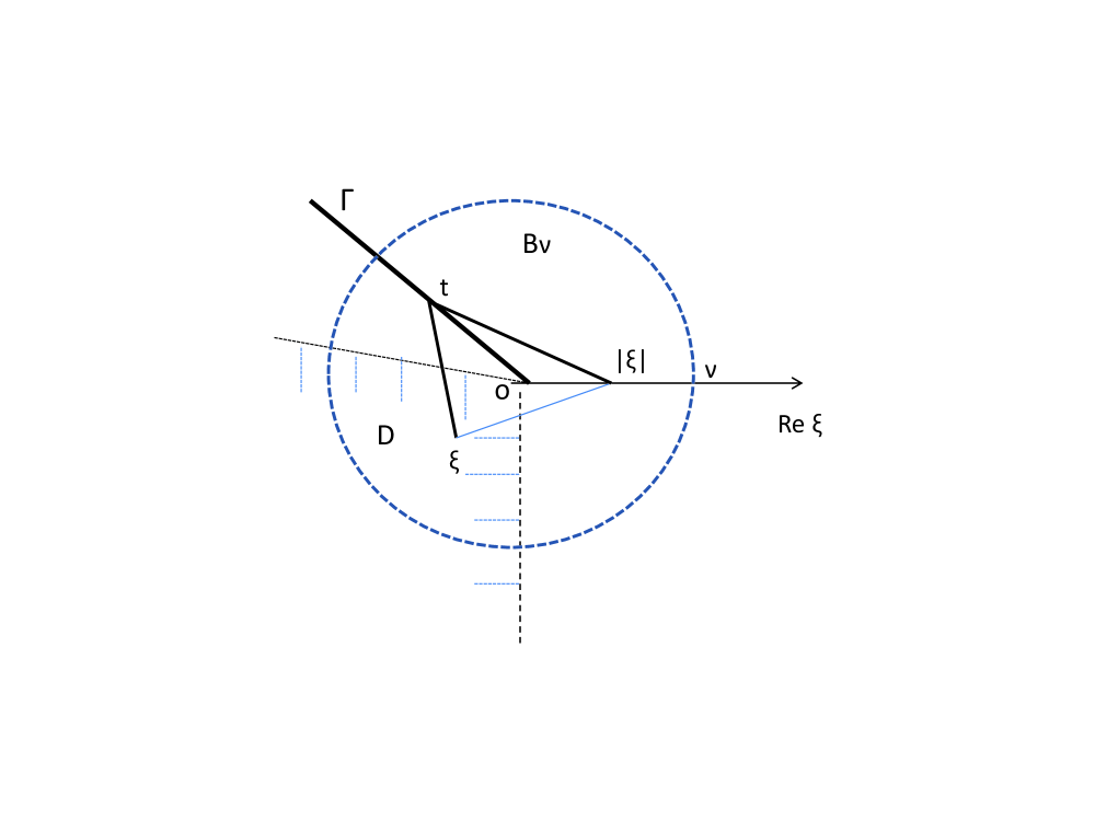
Figure 4. Relevant to (2.19) in Lemma 2.15 and Remark 2.16

Remark 2.16.

Note if $\Gamma$ is in $\mathcal{D}_{c}^{\prime}$, an angular subset of $\mathcal{D}_{c}$ (complement of $\mathcal{D}$), then (2.19) hold (see Fig: 4).

Definition 2.17.

Define

(2.23) $$\begin{split}\Omega_{0}=\biggl{\{}\xi:\xi\text{ is below }\{\xi=\rho e^{i(\pi-\varphi_{0}-\frac{1}{3}\mu)}\}\\ \cup\{\xi=\rho e^{i(\varphi_{0}+\frac{1}{3}\mu)}\}\biggr{\}}.\end{split}$$

Remark 2.18.

$\mathcal{R}\cup\{\text{ Im }\xi<0\}$ is an angular subset of $\Omega_{0}$, and $\Omega_{0}$ is itself an angular subset of the region $\{\xi\text{ below }r_{0}\}$.

Lemma 2.19.

Let $F\in\mathbf{A}_{0}^{-}$, then

$$\underset{\xi\in\Omega_{0}/B_{\nu}}{\sup}\lvert(\xi-2i)^{k+\tau}F_{-}^{(k)}(\xi)\rvert\leq K_{2}\frac{\underset{\xi\in\mathcal{R}/B_{\nu}}{\sup}~{}|(\xi-2i)^{\tau}F|}{|\nu|^{k}},~{}k=0,1,2,$$

and

$$\underset{\xi\in\overline{\Omega_{0}\cap B_{\nu}}}{\sup}~{}\left|\frac{F^{\prime}_{-}(\xi)-F^{\prime}_{-}(0)}{\sqrt{\xi}}\right|\leq K_{2}\left(\underset{\xi\in\overline{\mathcal{R}^{-}\cap B_{\nu}}}{\sup}~{}\left|\frac{F^{\prime}(\xi)-F^{\prime}(0)}{\sqrt{\xi}}\right|+|\nu|^{-3/2}\underset{\xi\in\mathcal{R}/B_{\nu}}{\sup}~{}|F|\right),$$

where constant $K_{2}$ depends only on $\varphi_{0}$.

Proof.

From Remarks 2.16-2.18, conditions (2.16)-(2.18) hold with $\Gamma=r_{0}$ and $\mathcal{D}$ = $\Omega_{0}$. Using $\lVert\bar{F}\rVert_{0,r_{0}^{-}}\leq\lVert F\rVert_{0}^{-}$, (2.18) and applying Lemma 2.15, with $g=\bar{F}^{\prime}$, we obtain the proof. ∎

Remark 2.20.

From now on, we choose $F\in\mathbf{A}_{0,\delta}^{-},$ with additional restriction,

(2.24) $$\delta<\frac{K_{3}}{2}\equiv\frac{H_{m}}{2KK_{2}},$$

where $H_{m},K$ are as in (2.5) with $\mathcal{D}=\mathcal{R}$, while $K_{2}$ is defined as in Lemma 2.19. This ensures

(2.25) $$|\xi-2i||F^{\prime}_{-}+\bar{H}|\geq(H_{m}-K\lVert F^{\prime}_{-}\rVert_{1,\mathcal{D}})\geq(H_{m}-KK_{2}\lVert F\rVert_{0})\geq C\frac{K_{3}}{2}>0;$$

so $F^{\prime}_{-}+\bar{H}\neq 0$ in $\mathcal{R}$. On the other hand, from Cauchy Integral Formula and Lemma 2.12 in [38], we have $\lVert F^{\prime}\rVert_{1,\mathcal{D}}\leq C\lVert F\rVert_{0}\leq\frac{K_{1}}{2}$. Therefore from Remark 2.8, $G(F,F_{-})$ is analytic in $\mathcal{D}^{\prime}$ which is subdomain of $\mathcal{R}$ and contains the real $\xi$ axis .

Remark 2.21.

Using Lemmas 2.5 and 2.19, $G(F,F_{-})(t)~{}=~{}O(t^{-\tau})$ as $|t|\to\infty,t$ in any angular subset of $\mathcal{R}\cap\Omega_{0}$ including the real axis.

Definition 2.22.

If $F\in\mathbf{A}_{0,\delta}$, define operator $I_{1}(F)$ so that for Im $\xi<0$,

(2.26) $$I_{1}(F)[\xi]=-\frac{1}{2\pi}\int_{-\infty}^{\infty}\frac{G(F,F_{-})(t)}{t-\xi}dt.$$

Lemma 2.23.

If $F\in\mathbf{A}_{0,\delta}$ and $F$ is analytic in $\mathrm{Im}~{}\xi~{}>~{}0$ and also satisfies (1.14), then in the region $\{~{}\mathrm{Im}~{}\xi<0~{}\}\cap\mathcal{R}$, $F$ satisfies

(2.27) $$F^{\prime}(\xi)~{}=~{}\frac{1}{2\epsilon^{4}}\big{\{}-\big{[}G_{2}(F,I_{1})^{2}(F_{-}^{\prime}+\bar{H})+2\epsilon^{4}G_{1}(F^{\prime}_{-})\big{]}\\ +(F_{-}^{\prime}+\bar{H})G_{2}(F,I_{1})\sqrt{G_{2}(F,I_{1})^{2}-4\epsilon^{4}}\big{\}}.$$

Proof.

Since conditions of Lemma 2.10 are satisfied, (2.9) holds. Since $F$ is analytic in $\mathcal{R}\cup\{\text{Im }\xi>0\}$ with property (1.17), from Lemma 2.14, $F_{-}={\bar{F}}$; hence $I_{1}(F)(\xi)=I(F)(\xi)$. Therefore (2.9) implies (2.27). ∎

Lemma 2.24.

If $F\in\mathbf{A}_{0,\delta}$, and $F$ satisfies equation (2.27) in $\mathcal{R}\cap\{~{}\mathrm{Im}~{}\xi<0~{}\}$, then $F$ is analytic in $\mathcal{R}\cup\{~{}\mathrm{Im}~{}\xi>0~{}\}$ and satisfies (1.14) on the real $\xi$ axis.

Proof.

Note on using expression from (2.26), (2.27) can be rewritten as:

(2.28) $$F(\xi)=-\epsilon^{2}I_{1}(F)(\xi)+i\epsilon^{2}G(F,F_{-})[\xi]\quad\text{for Im }~{}\xi<0,$$

where operator $G$ is defined by (2.3). Analytically continuing the above equation to the upper half plane, we have:

(2.29) $$F(\xi)=\frac{\epsilon^{2}}{2\pi}\int_{-\infty}^{\infty}\frac{G(F,F_{-})(t)dt}{t-\xi}\quad\text{~{}for Im }\xi>0;$$

so $F(\xi)$ is analytic in the upper half plane. From Lemma 2.14, $F_{-}(\xi)={\bar{F}}(\xi)$; hence on the real $\xi$-axis, $F_{-}(\xi)=F^{*}(\xi)$. Equation (2.29) reduces to:

$$F(\xi)=-\frac{\epsilon^{2}}{\pi i}\int^{\infty}_{-\infty}\frac{dt}{t-\xi}\frac{1}{\lvert F^{\prime}(t)+H(t)\rvert^{1/2}}\text{ Im }\left[F^{\prime}(t)+H(t)\right]\qquad~{}\text{ for Im ~{}}\xi>0.$$

On taking the limit Im  $\xi~{}\rightarrow~{}0^{+}$, the above implies (1.14). ∎

Because of Remark 1.10 about equivalence of condition (iii) to Im  $F=0$ on $\{\text{ Re ~{}}\xi=0\}\cap\mathcal{R}$, Lemmas 2.23 and 2.24 imply:

Theorem 2.25.

The finger problem is equivalent to
Problem 1: Find function $F\in\mathbf{A}_{0,\delta}$, satisfying $\mathrm{Im}~{}F~{}=~{}0$ on $\left\{~{}\mathrm{Re}~{}\xi=0\right\}\cup\mathcal{R}$, so that (2.27) is satisfied in $\mathcal{R}\cap\{~{}\mathrm{Im}~{}\xi<0\}$.

2.2. Formulation of Problem 2

Let $\alpha_{1}>0$ be a fixed constant independent of $\epsilon$ so that $-\alpha_{1}i\in\mathcal{R}$.

Definition 2.26.

Define two rays

$$r^{+}_{1}=\{\xi:\xi=-\alpha_{1}i+\rho e^{-i\varphi_{0}},0<\rho<\infty\},$$

$$r^{-}_{1}=\{\xi:\xi=-\alpha_{1}i+\rho e^{i(\pi+\varphi_{0})},0<\rho<\infty\}.$$

$r_{1}=r_{1}^{-}\cup r_{1}^{+}$ is a directed contour from left to right (see Fig.5).

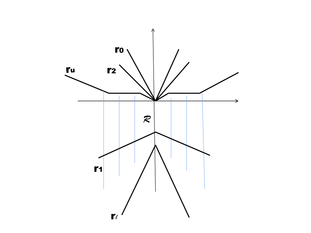
Figure 5. Rays defined in Subsection 2.2.

Definition 2.27.

Let $F\in\mathbf{A}_{0,\delta}$. For $\xi$ above $r_{1}$, define

(2.30) $$F_{+}(\xi)=\frac{1}{2\pi i}\int_{r_{1}}\frac{F(t)dt}{t-\xi}.$$

Remark 2.28.

$F_{+}$ as defined above is analytic for $\xi$ above $r_{1}$. Also, it is to be noted that for $F\in\mathbf{A}_{0}^{-}$ only, when $F(\xi)=[F(-\xi^{*})]^{*}$ is invoked to define $F$ on $\mathcal{R}^{+}$, we can write

(2.31) $$\begin{split}F_{+}(\xi)&=\frac{1}{2\pi i}\left[\int_{r_{1}^{-}}\frac{F(t)dt}{t-\xi}+\int_{r_{1}^{+}}\frac{[F(-t^{*})]^{*}dt}{t-\xi}\right]\\ &=~{}\frac{1}{2\pi i}\int_{r_{1}^{-}}\left[\frac{F(t)dt}{t-\xi}-\frac{[F(t)]^{*}dt^{*}}{t^{*}+\xi}\right].\end{split}$$

This expression is equivalent to (2.30) when the symmetry condition: Im  $F~{}=~{}0$ on $\{\text{ Re ~{}}\xi=0\}\cap\mathcal{R}$ is satisfied. However, even without symmetry, (2.31) still defines an analytic function for $\xi$ above $r_{1}$, with possible singularity at $\xi=-i\alpha_{1}$. It is easy to see that $F_{+}(\xi)$ satisfies the symmetry condition on $\{\text{ Re ~{}}\xi=0\}\cup\mathcal{R}\cup\{\text{ Im ~{}}\xi>-\alpha_{1}\}$ even when $F$ does not. Further, if $F\in\mathbf{A}_{0}$ is also analytic in $\{\text{ Im ~{}}\xi~{}>~{}0\}$, then it is clear from (2.30) on closing the contour from the top that $F_{+}(\xi)=F(\xi)$.

Definition 2.29.

Define

(2.32) $$\Omega_{1}=\bigg{\{}\xi:\xi\text{ is above }~{}\{\xi=-\frac{\alpha_{1}}{2}i+\rho e^{i(\pi+\frac{\varphi_{0}}{2})}\}\cup\{\xi=-\frac{\alpha_{1}}{2}i+\rho e^{-i\frac{\varphi_{0}}{2}}\}\bigg{\}}.$$

Remark 2.30.

$\Omega_{1}$ is an angular subset of the region $\{\xi:\xi\text{ above }r_{1}\}$, $r_{1}$ as in Definition 2.26.

Lemma 2.31.

Let $F\in\mathbf{A}_{0,\delta}^{-},F^{\prime}\in\mathbf{A}_{1,\delta_{1}}^{-}$, then

$$\underset{\xi\in\Omega_{1}}{\sup}\left\lvert(\xi-2i)^{k+\tau}F_{+}^{(k)}(\xi)\right\rvert\leq K_{2}\lVert F\rVert_{0}^{-}\quad\text{ for }k=0,1,2,$$

where $K_{2}>0$ is independent of $\epsilon$, $\lambda$.

Proof.

The proof is very similar to that of Lemma 2.19. From Remarks 2.16-2.30, conditions (2.16)-(2.18) hold with $\Gamma=r_{1}$ and $\mathcal{D}$ = $\Omega_{1}$. Using $\lVert\bar{F}\rVert_{0,r_{0}^{-}}\leq\lVert F\rVert_{0}^{-}$, (2.31) and applying Lemma 2.15, with $g=F$, we obtain the proof. ∎

Definition 2.32.

We define two rays (see Figure 5):

$$r^{+}_{2}=\{\xi:\xi=\rho e^{i\varphi_{0}+\frac{1}{4}\mu},0<\rho<\infty\},$$

$$r^{-}_{2}=\{\xi:\xi=\rho e^{i(\pi-\varphi_{0}-\frac{1}{4}\mu)},0<\rho<\infty\}.$$

$r_{2}$ is a directed contour from left to right on the path $r_{2}^{-}\cup r_{2}^{+}$.

Remark 2.33.

$r_{2}$ is an angular subset of $\Omega_{0}\cap\Omega_{1}$ and $\mathcal{R}$ is below $r_{2}$.

Definition 2.34.

If $F\in\mathbf{A}_{0,\delta}^{-}$, let $F^{\prime}_{-}$ be given by (2.18) and $F_{+}$ as in (2.30). Define operator $I_{2}$ so that

(2.33) $$I_{2}(F)[\xi]=-\frac{1}{2\pi}\int_{r_{2}}\frac{G(F_{+},F_{-})(t)dt}{t-\xi}\qquad\text{for }\xi\text{ below }r_{2}.$$

Remark 2.35.

Because of Lemmas 2.5, 2.19 and 2.31, $G(F_{+},F_{-})(t)\sim O(t^{-\tau})$ as $|t|\to\infty$ and analytic for $t$ in any angular subset of $\Omega_{0}\cap\Omega_{1}$ that includes $r_{2}$; so $I_{2}(F)[\xi]$ is analytic below $r_{2}$. Also, from the symmetry of each of $F_{+}$ and $F_{-}$, it is not difficult to see that $I_{2}(F)[\xi]$ also satisfies the symmetry condition on $\{\text{ Re ~{}}\xi=0\}\cap\mathcal{R}$.

Lemma 2.36.

Let $F\in\mathbf{A}_{0,\delta}^{-}$. Then $I_{2}(F)\in\mathbf{A}$, and $\lVert I_{2}(F)\rVert_{0}\leq K_{5},$ where $K_{5}>0$ is independent of $\epsilon$ and $\lambda$.

Proof.

From Lemma 2.19 and Lemma 2.31,

$$\lVert F_{-}^{(k)}\rVert_{k,r_{2}}\leq K_{2}\lVert F\rVert_{0}^{-}~{}~{},~{}~{}\lVert F_{+}^{(k)}\rVert_{k,r_{2}}\leq K_{2}\lVert F\rVert_{0}^{-}.$$

Applying Lemma 2.5 (with $\mathcal{D}=r_{2}$) and Lemma 2.15 (with $\Gamma=r_{2}$ and $\mathcal{D}=\mathcal{R}$) to (2.33), we complete the proof. ∎

Lemma 2.37.

If $F\in\mathbf{A}_{0,\delta},$ and $F$ satisfies (2.27) in $\mathcal{R}\cap\{~{}\mathrm{Im}~{}\xi<0\}$, then for $\xi\in\mathcal{R}$, $F$ satisfies

(2.34) $$F^{\prime}(\xi)~{}=~{}\frac{1}{2\epsilon^{4}}\big{\{}-\big{[}G_{2}(F,I_{2})^{2}(F_{-}^{\prime}+\bar{H})+2\epsilon^{4}G_{1}(F^{\prime}_{-})\big{]}\\ +(F^{\prime}_{-}+\bar{H})G_{2}(F,I_{2})\sqrt{G_{2}(F,I_{2})^{2}-4\epsilon^{4}}\big{\}}.$$

Proof.

If $\delta$ is small enough, from Lemmas 2.19 and 2.31, $|(\xi-2i)^{1+\tau}F_{-}^{\prime}|$ and $|(\xi-2i)^{1+\tau}F^{\prime}_{+}|$ are each small in the domain $\Omega_{0}\cap\Omega_{1}$ which contains the region between $r_{2}$ and $r_{1}$; hence $F_{-}^{\prime}+\bar{H}\neq 0$ and $F_{+}^{\prime}+H~{}\neq 0$ in that domain. From Lemma 2.24, $F$ is analytic in $\{\text{ Im ~{}}\xi~{}>~{}0\}$; hence $F_{+}=F$. By deforming the contour $r_{2}$ in (2.33) back to the real axis, it follows $I_{2}(F)(\xi)=I_{1}(F)(\xi)$, for Im $\xi<0$. By analytic continuation, $F$ satisfies (2.34) for $\xi\in\mathcal{R}$. ∎

Problem 2: Find function $F\in\mathbf{A}_{0,\delta}^{-}$ so that $F$ satisfies the symmetry condition Im  $F=0$ on $\mathcal{R}\cap\left\{~{}\text{Re ~{}}\xi=0\right\}$ and equation (2.34) in $\mathcal{R}^{-}$.

Theorem 2.38.

Let $F\in\mathbf{A}_{0,\delta}^{-}$. If $F(\xi)$ satisfies the symmetry condition $\mathrm{Im}~{}F=0$ on $\mathcal{R}\cap\left\{~{}\mathrm{Re}~{}\xi=0\right\}$ and the equation (2.34) in $\mathcal{R}^{-}$, then for sufficiently small $\epsilon$ and $\delta$ , $F$ is a solution to Problem 1 (and hence a solution to the original Finger Problem).

The proof of Theorem 2.38 will be given later after several lemmas.

Lemma 2.39.

Assume $F\in\mathbf{A}_{0,\delta}^{-}$ and $F$ satisfies the integral equation (2.34) in $\mathcal{R}^{-}$ as well as the symmetry condition $\mathrm{Im}~{}F(\xi)=0$ for $\xi\in\{~{}\mathrm{Re}~{}\xi=0\}\cap\mathcal{R}$. Let $U(\xi)=F(\xi)-F_{+}(\xi)$, then
(1) $U(\xi)$ is analytic in $\mathcal{R}\cap\{~{}\mathrm{Im}~{}\xi>0\}$.
(2) For $\xi\in\mathcal{R}^{-}\cap\{~{}\mathrm{Im}~{}\xi~{}>~{}0\}$, $U$ satisfies:

(2.35) $$\epsilon^{2}U^{\prime}(\xi)+\tilde{Q}(\xi)U(\xi)=\bar{M}(U)+M(U),$$

where

(2.36) $$\tilde{Q}(\xi)=\frac{2iH^{3/2}\bar{H}^{1/2}}{H+\bar{H}}=i\frac{(\xi+i\gamma)^{3/2}(\xi-i\gamma)^{1/2}}{\xi(\xi^{2}+1)},$$

(2.37) $$\begin{split}&\bar{M}(\xi)=\bar{M}(U)[\xi]\equiv[-iR_{1}(\xi)+\tilde{Q}(\xi)]U,\\ &M(U)(\xi):=-\frac{\epsilon^{2}i}{2\pi}\mathcal{R}_{1}(\xi)\int_{-\infty}^{\infty}\frac{\mathcal{R}_{1}^{-1}(t)U^{\prime}(t)}{t-\xi}dt\qquad\text{for $\mathrm{Im}~{}\xi~{}>~{}0$},\end{split}$$

$\mathcal{R}_{1}(\xi)=R_{1}(F,F_{-},F_{+})[\xi]$, where operator $R_{1}$ is defined by:

(2.38) $$R_{1}(F,F_{-},F_{+})\\ =\frac{[(F^{\prime}_{+}+H)^{1/2}+(F^{\prime}+H)^{1/2}](F_{+}^{\prime}+H)^{1/2}(F^{\prime}+H)^{1/2}(F_{-}^{\prime}+\bar{H})^{1/2}}{[(F^{\prime}_{-}+\bar{H})+(F^{\prime}+H)^{1/2}(F_{+}^{\prime}+H)^{1/2}]}.$$

Proof.

Since each of $F$ and $F_{+}$ are analytic in $\mathcal{R}\cap\{~{}\text{ Im ~{}}\xi>0\}$, it follows that $U=F-F_{+}$ is also analytic in $\mathcal{R}\cap\{\text{ Im ~{}}\xi>0\}$; hence statement (1) follows. Since $F$ satisfies (2.34) in $\mathcal{R}^{-}$, the symmetry condition and the Schwarz reflection principle that relates $F$ and its derivatives in $\mathcal{R}^{+}$ to their values in $\mathcal{R}^{-}$ guarantees that (2.34) is satisfied in $\mathcal{R}$. But equation (2.34) can be rewritten as:

(2.39) $$F(\xi)=-\epsilon^{2}I_{2}(\xi)+i\epsilon^{2}G(F,F_{-})(\xi).$$

Then, on deforming the contour for $I_{2}$ from $r_{2}$ to $(-\infty,\infty)$,

(2.40) $$F(\xi)=-\epsilon^{2}I_{3}(\xi)-i\epsilon^{2}\left[G(F_{+},F_{-})(\xi)-G(F,F_{-})(\xi)\right]~{}\text{ for $\xi$ above $(-\infty,\infty)$},$$

where

(2.41) $$I_{3}(\xi)=-\frac{1}{2\pi}\int_{-\infty}^{\infty}\frac{G(F_{+},F_{-})(t)}{t-\xi}dt\qquad\text{for $\xi$ above $r_{1}$ }.$$

It is clear that $I_{3}(\xi)$ is analytic above $r_{1}$; indeed from contour deformation of (2.30) and (2.41) and analyticity and decay properties of $G(F_{+},F_{-})$ on $\mathcal{R}$ itself, it is clear that $I_{3}\in\mathbf{A}_{0}$ and analytic in $\mathcal{R}\cup\{~{}\text{ Im ~{}}\xi~{}>~{}0\}$. Substituting for $F$ from (2.41) into (2.34), it follows that for Im  $\xi~{}>~{}0$,

(2.42) $$\begin{split}&F_{+}(\xi)=-\epsilon^{2}I_{3}(\xi)-\frac{\epsilon^{2}}{2\pi}\int_{-\infty}^{\infty}\frac{[G(F_{+},F_{-})[t]-G(F,F_{-})[t]]}{t-\xi}dt\\ &=\frac{\epsilon^{2}}{2\pi}\int_{-\infty}^{\infty}\frac{G(F,F_{-})(t)}{t-\xi}dt~{}~{}\qquad\text{for $\text{ Im ~{}}\xi>~{}0$}.\end{split}$$

Subtracting (2.42) from (2.40), we obtain for Im  $\xi~{}>~{}0$:

(2.43) $$\begin{split}U(\xi)~{}=~{}&-i\epsilon^{2}\left[G(F_{+},F_{-})(\xi)-G(F,F_{-})(\xi)\right]\\ &~{}+\frac{\epsilon^{2}}{2\pi}\int_{-\infty}^{\infty}\frac{G(F_{+},F_{-})(t)-G(F,F_{-})(t)}{t-\xi}dt.\end{split}$$

Using (2.3), and the definition of $G_{1}$ and $G_{4}$ in (2.41) and (2.38),

(2.44) $$G(F,F_{-})-G(F_{+},F_{-})=R_{1}^{-1}(F,F_{-})U^{\prime}.$$

From (2.44), (2.43), $U(\xi)$ satisfies the equation (2.35) for Im  $\xi~{}>~{}0$.

∎

Definition 2.40.

We define two rays $r_{3}^{-}$ and $r_{3}^{+}$:

$$r_{3}^{-}=\{\xi:\xi=re^{i\left(\pi-\frac{\phi_{0}}{2}\right)},r>0\},$$

$$r_{3}^{+}=\{\xi:\xi=re^{\frac{i\phi_{0}}{2}},r>0\};$$

and $\Omega_{3}$ is defined to be the region between $r_{3}=r_{3}^{-}\cup r_{3}^{+}$ and $r_{u}$.

Definition 2.41.

We define

(2.45) $$g_{1}(\xi)=\exp\left(-\frac{P(\xi)}{\epsilon^{2}}\right),$$

(2.46) $$g_{2}(\xi)=\exp\left(\frac{P(\xi)}{\epsilon^{2}}\right),$$

where

(2.47) $$P(\xi)~{}=~{}\int^{\xi}\tilde{Q}(t)dt~{}=~{}\int i\frac{(\xi+i\gamma)^{3/2}(\xi-i\gamma)^{1/2}}{\xi(\xi^{2}+1)}d\xi.$$

Lemma 2.42.

Let $U$ be as in Lemma 2.39 , then $U$ satisfies

(2.48) $$U=\frac{1}{\epsilon^{2}}g_{1}(\xi)\int_{\infty}^{\xi}(\bar{M}(t)+M(t))g_{2}(t)dt.$$

Proof.

Since $U$ satisfies (2.35), we have

$$U(\xi)=Cg_{1}(\xi)+\frac{1}{\epsilon^{2}}g_{1}(\xi)\int_{\infty}^{\xi}(\bar{M}(t)+M(t))g_{2}(t)dt.$$

$C$ has to be zero since $U(\infty)=0$ and $g_{1}(\infty)\neq 0$ from Lemma 6.1. ∎

Remark 2.43.

We will show that $U=0$. Since $F$, $F^{+}$ and hence $U$ is known to be analytic in $\mathcal{R}$ and continuous upto its boundary, it is enough to show that $U=0$ on $\Omega_{3}^{-}$. We will do so by showing that equation (2.48) forms a contraction map in the space of functions $U$ on $\Omega_{3}^{-}$, with norm

$$\|U\|_{\Omega_{3}}=\sup_{\xi\in\Omega_{3}}~{}|\xi-2i|^{\tau}|U(\xi)|+\epsilon^{2}\underset{\overline{B_{\nu}\cap\Omega_{3}}}{\sup}~{}\left|\frac{U^{\prime}(t)-U^{\prime}(0)}{\sqrt{t}}\right|+|U^{\prime}(0)|$$

It is to be noted that the integration in (2.48) can be performed on the path $\mathcal{P}(\xi,\infty)$ contained in $\Omega_{3}^{-}$, so that on this path on any $\mathbf{C}^{1}$ segment, $\frac{d}{ds}~{}\text{Re}~{}P(t(s))~{}<~{}0$ for arc length $s$ increasing in the direction of $\infty$, Lemmas 2.50-2.53 are valid and hence the integral operator in (2.48) is bounded when restricted to functions on $\Omega_{3}^{-}$. Further note that since $U$ are analytic in $\mathcal{R}\cup\{~{}\text{Im ~{}}\xi~{}<~{}0\}$ and satisfies the symmetry condition, it follows that $U$ on $\Omega_{3}^{-}$ completely determines $U$ and its derivatives for $\xi$ real. This is crucial in controlling $\mathcal{M}$ on $r_{3}^{-}$, as necessary.

Lemma 2.44.

Let $F\in\mathbf{A}_{0,\delta}$, then for $\xi\in\mathcal{R}$

(2.49) $$|R_{1}(F,F_{-})(\xi)|\leq C/|\xi-2i|,~{}|1/R_{1}(F,F_{-})(\xi)|\leq C|\xi-2i|,$$

where $C$ is independent of $\epsilon$ and $\lambda$.

Proof.

The lemma follows from (2.38) and Lemma 2.39. ∎

Lemma 2.45.

Let $U(\xi)$ be as in Lemma 2.39, then

(2.50) $$\underset{\xi\in\mathcal{D}}{\sup}~{}|\xi-2i|^{1+\tau}|U^{\prime}|(\xi)|\leq\frac{C}{|\nu|}\lVert U\rVert_{0,r_{3}^{-}}~{},~{}~{}$$

where $\mathcal{D}=(-\infty,-\nu)$, $C$ is independent of $\epsilon$ and $\lambda$.

Proof.

Since $U$ is analytic in the region under $r_{3}$ and continuous upto its boundary, by the Cauchy Integral Formula:

$$U^{\prime}(\xi)=-\frac{1}{2\pi i}\int_{r_{3}}\frac{U(t)}{(t-\xi)^{2}}dt\qquad\text{for $\xi$ in $\mathcal{D}$ }.$$

Applying Lemma 2.11 in [38], with $\Gamma$ chosen to be $r_{u}$, we have $|\xi-2i|^{1+\tau}|U^{\prime}|(\xi)|\leq C\lVert U\rVert_{0,r_{3}^{-}}$ for $\xi\in(-\infty,-3)$ .
For $\xi\in(-\infty,-3)$, we split the integral into

$$\begin{split}U^{\prime}(\xi)&=-\frac{1}{2\pi i}\left(\int_{r_{3}\cap B_{3}}+\int_{r_{3}/B_{3}}\right)\frac{U(t)}{(t-\xi)^{2}}dt\\ &=:U_{1}+U_{2}.\end{split}$$

Applying Lemma 2.11 in [38], with $\Gamma$ chosen to be $r_{u}/B_{3}$, we have $|U_{2}|(\xi)|\leq C\lVert U\rVert_{0,r_{3}^{-}}$ for $\xi\in(-3,-\nu)$ .
For $t=re^{\theta}\in r_{3}\cap B_{3}$ and $\xi\in(-3,-\nu)$, using $|t-\xi|^{2}=(r\cos\theta-\xi)^{2}+r^{2}\sin^{2}\theta$, we have

$$\begin{split}|U_{1}(\xi)|&=\left|-\frac{1}{2\pi i}\int_{r_{3}\cap B_{3}}\frac{U(t)}{(t-\xi)^{2}}dt\right|\\ &\leq C\left|\int_{0}^{3}\frac{\underset{r_{3}}{\sup}|U(t)|}{(r\cos\theta-\xi)^{2}+r^{2}\sin^{2}\theta}dr\right|\leq C\frac{\underset{r_{3}}{\sup}~{}|U(t)|}{|\xi|};\end{split}$$

hence the lemma follows.

∎

Lemma 2.46.

Let $U(\xi)$ be as in Lemma 2.39, then

(2.51) $$\underset{\xi\in(-\nu,0)}{\sup}|U^{\prime}(\xi)-U^{\prime}(0)|\leq\frac{C\sqrt{|\xi|}}{|\nu|^{3/2}}~{}\lVert U\rVert_{\Omega_{3}},$$

$C>0$ is independent of $\epsilon$ and $\lambda$.

Proof.

$$U^{\prime}(\xi)=-\frac{1}{2\pi i}\int_{r_{4}}\frac{U^{\prime}(t)}{(t-\xi)}dt\text{ for $\xi$ in $(-\nu,0)$ },$$

where $r_{4}$ is a line between $r_{3}$ and $r_{u}$ defined by

$$r_{4}^{-}=\{\xi:\xi=re^{i(\pi-2\phi_{0}/3)},r>0\},$$

$$r_{4}^{+}=\{\xi:\xi=re^{i(2\phi_{0}/3)},r>0\}.$$

Applying Lemma 2.15, we obtain

$$|U^{\prime}(\xi)-U^{\prime}(0)|\leq C\sqrt{|\xi|}\left(\frac{\underset{r_{4}/B_{\nu}}{\sup}|U^{\prime}(t)|}{\sqrt{|\nu|}}+\lVert U\rVert_{0,r_{4}}\right).$$

From Cauchy integral formula, for $t\in r_{4}/B_{\nu}$ we have

$$U^{\prime}(t)=-\frac{1}{2\pi i}\int_{\partial\Omega_{3}}\frac{U(s)}{(s-t)^{2}}ds;$$

since $|t-s|\geq C||s|e^{i\theta}-|t||$, for $t\in r_{4}/B_{\nu}$ and $s\in\partial\Omega_{3}$ we have

$$\underset{r_{4}/B_{\nu}}{\sup}|U^{\prime}(t)|\leq C\frac{\underset{\partial\Omega}{\sup}~{}|U(s)|}{|\nu|};$$

hence the lemma follows. ∎

Lemma 2.47.

Let $U(\xi)$ be as in Lemma 2.39, then $\underset{(-\nu,0)}{\sup}~{}|U^{\prime}(\xi)|\leq\frac{C}{|\nu|}~{}\lVert U\rVert_{\Omega_{3}}$, where $C>0$ is a constant independent of $\epsilon$ and $\lambda$.

Proof.

The lemma follows from the Cauchy Integral Formula and the above lemma. ∎

Lemma 2.48.

Let $F\in\mathbf{A}_{0,\delta}$. Let ${\bar{M}}(U)$ and $M(U)$ be as defined in (2.37), then

(2.52) $$|{\bar{M}}(U)(\xi)|\leq C\delta_{2}(1+|\xi|)^{-1-2\tau}\lVert U\rVert_{\Omega_{3}},$$

(2.53) $$|M(U)(\xi)|\leq C\frac{\epsilon^{2}}{|\nu|^{2}}(1+|\xi|)^{-1-\tau}\lVert U\rVert_{\Omega_{3}}\qquad\text{ for }\xi\in\Omega/B_{\nu},$$

(2.54) $$\left|\frac{d}{d\xi}M(U)(\xi)\right|\leq C\frac{\epsilon^{2}}{|\nu|^{2}}(1+|\xi|)^{-2-\tau}\lVert U\rVert_{\Omega_{3}}\qquad\text{ for }\xi\in\Omega/B_{\nu},$$

and

(2.55) $$\underset{\xi\in(-\nu,0)}{\sup}~{}|M^{\prime}(\xi)-M^{\prime}(0)|\leq\frac{C\sqrt{|\xi|}}{|\nu|^{2}}\lVert U\rVert_{\Omega_{3}}\qquad\text{ for }\xi\in\Omega_{3}\cap B_{\nu},$$

where $C$ is some constant independent of $\epsilon$ and

(2.56) $$\delta_{2}=\bigg{\{}\left(\lVert F\rVert_{0}+1\right)^{1/2}-1\bigg{\}}.$$

Proof.

The (2.52) follows from

(2.57) $$|(-iR_{1}+\tilde{Q})|\leq C|t-2i|^{-1-\tau}\delta_{2}~{}\qquad\text{for $t\in\Omega_{3}$}.$$

Using Lemma 2.44 and Lemma 2.45:

(2.58) $$|R_{1}^{-1}U^{\prime}(t)|\leq\frac{C}{|\nu|}|t-2i|^{-\tau}\lVert U\rVert_{0}~{}\qquad\text{for $t\in(-\infty,-\nu)$}.$$

Applying Lemmas 2.15, and Lemmas 2.44 - 2.45 to (2.37), we obtain (2.53) and (2.54). (2.55) follows from Lemmas 2.45 - 2.47. ∎

Definition 2.49.

Let $\mathcal{Q}$ be any connected set in the complex $\xi$-plane, we introduce norms: $\lVert F(\xi)\rVert_{j,\mathcal{Q}}:=\underset{\xi\in\mathcal{Q}}{\sup}~{}\lvert(\xi-2i)^{j+\tau}F(\xi)\rvert,j=0,1,2$; and $\mathbf{C}(\mathcal{Q})$ is the function space of all continuous functions on $\mathcal{Q}$.

In order to prove Theorem 2.38 using the strategy described in Remark 2.43, we need to control the integral operator in equation (2.48). Due to the properties of $P(\xi)$ (see the appendix), we need to break the integral from $0$ to $\infty$ into several integrals along special paths, each of these integrals then can be estimated accordingly (see Lemmas 2.50 - 2.54 below).

Lemma 2.50.

If $N\in\mathbf{C}(\mathcal{Q}),N^{\prime}\in\mathbf{C}(\mathcal{Q})$ where $\mathcal{Q}$ is a path $\mathcal{P}(\xi,\infty)$ on which $\mathrm{Re}~{}(P(t)-P(\xi))$ decreases monotonically as $\mathrm{Re}~{}t$ increases. Let

(2.59) $$f_{1}(\xi):=\frac{1}{\epsilon^{2}}g_{1}(\xi)\int^{\xi}_{\infty}N(t)g_{2}(t)dt.$$

Then $f_{1}(\xi)\in\mathbf{C}(\mathcal{Q})$ and

(2.60) $$\lVert f_{1}\rVert_{0}\leq\frac{C}{\epsilon^{2}}~{}\lVert N\rVert_{1},$$

and $\lVert f_{1}\rVert_{0}\leq C~{}(\lVert N\rVert_{1}+\lVert N^{\prime}\rVert_{2}),$ where $C$ is independent of $\epsilon$ and $\lambda$.

Proof.

$$|f_{1}(\xi)|=\left\lvert\frac{1}{\epsilon^{2}}\int_{\mathcal{P}(\xi,\infty)}N(t)\exp\{-\frac{1}{\epsilon^{2}}(P(\xi)-P(t))\}dt\right\rvert\\ \leq\frac{1}{\epsilon^{2}}\lVert N\rVert_{1}\int^{\infty}_{|\xi|}|(t-2i)^{-1-\tau}|dt\leq\frac{C}{\epsilon^{2}}\lVert N\rVert_{1}|\xi-2i|^{-\tau}.$$

By integration by parts, we have

$$|f_{1}(\xi)|=\left\lvert\frac{1}{\epsilon^{2}}\int_{\mathcal{P}(\xi,\infty)}N(t)\exp\{-\frac{1}{\epsilon^{2}}(P(\xi)-P(t))\}dt\right\rvert\\ =\left\lvert\frac{1}{\epsilon^{2}}\int_{\mathcal{P}(\xi,\infty)}\frac{N(t)}{-\frac{d}{ds}P(t)}d\left(\exp\{-\frac{1}{\epsilon^{2}}(P(\xi)-P(t))\}\right)\right\rvert\\ \leq\lVert N\rVert_{1}\times\int^{\infty}_{0}\frac{|(t-2i)^{-1-\tau}||\frac{d^{2}}{dt^{2}}P(t)|}{|\frac{d}{dt}P(t)|^{2}}\left[\exp~{}\{-\frac{1}{\epsilon^{2}}\text{ Re }(P(\xi)-P(t))\}\right]dt\\ +\lVert N^{\prime}\rVert_{2}\times\int^{\infty}_{0}\frac{|(t-2i)^{-2-\tau}|}{|\frac{d}{dt}P(t)|}\left[\exp~{}\{-\frac{1}{\epsilon^{2}}\text{ Re }(P(\xi)-P(t))\}\right]dt.$$

Since

$$\left\lvert\frac{d}{dt}~{}~{}P(t)\right\rvert\geq C|t(s)-2i|^{-1},$$

$$\left\lvert\frac{d^{2}}{dt^{2}}~{}~{}P(t)\right\rvert\leq C|t(s)-2i|^{-2},$$

$$\frac{|(t-2i)^{-2-\tau}|}{\frac{d}{dt}P(t)}\leq C|\xi-2i|^{1-\tau},$$

we obtain $\lVert f_{1}\rVert_{0}\leq C(\lVert N\rVert_{1}+\lVert N^{\prime}\rVert_{2})$ and the lemma follows. ∎

If the estimate of the derivative of $N$ is not available and due to the factor $\frac{1}{\epsilon^{2}}$ in (2.60), Lemma 2.50 does not provide the estimate needed for the integral operator to be a contraction. By breaking up the integral and using properties of $P(\xi)$ ( Lemma 6.1, Lemma 6.3 and Lemma 6.6 in the appendix), we are able to obtain better estimates for the integral operator in the following two lemmas.

Lemma 2.51.

Let $R_{\epsilon}>R$ be a number which will be chosen later and be dependent on $\epsilon$. If $N(t)\leq C|t|^{-\sigma}$ for $t\in\mathcal{P}(\xi,R^{l}_{\epsilon})$, where $R^{l}_{\epsilon}=r_{l}^{-}\cap\{|\xi|=R_{\epsilon}\}$ and $\mathcal{P}(\xi,R^{l}_{\epsilon})\subset\mathcal{R}^{-}\cap\{R\leq~{}|\xi|\leq R_{\epsilon}\}$ is a path on which $\mathrm{Re}~{}(P(t)-P(\xi))$ decreases monotonically as $\mathrm{Re}~{}t$ increases, then

$$\begin{split}&f_{2}(\xi):=\frac{1}{\epsilon^{2}}g_{1}(\xi)\int^{\xi}_{R^{l}_{\epsilon}}N(t)g_{2}(t)dt\in\mathbf{C}\left(\mathcal{P}(\xi,R^{l}_{\epsilon})\right),\\ &\text{ and }\lVert f_{2}\rVert_{0}\leq C~{}R_{\epsilon}^{(2-\sigma+\tau)}\underset{\mathcal{P}(\xi,R^{l}_{\epsilon})}{\sup}(|t|^{\sigma}|N|),\end{split}$$

$C$ is independent of $\epsilon$ and $\lambda$.

Proof.

$$|f_{2}(\xi)|=\left\lvert\frac{1}{\epsilon^{2}}\int_{\mathcal{P}(\xi,R^{l}_{\epsilon})}N(t)\exp~{}\{-\frac{1}{\epsilon^{2}}(P(\xi)-P(t))\}dt\right\rvert\\ \leq\sup{(|t|^{\sigma}|N|)}\times\int^{1}_{0}\frac{|(t(s)|^{-\sigma}}{-\frac{d}{ds}\text{ Re }P(t(s))}d\left[\exp~{}\{-\frac{1}{\epsilon^{2}}\text{Re }(P(\xi)-P(t(s)))\}\right].$$

Since

$$-\frac{d}{ds}~{}\text{Re}~{}P(t(s))=-\text{ Re }\left(P^{\prime}(t)t^{\prime}(s)\right)\geq C|t(s)|^{-2},$$

$$\frac{|t(s)^{-\sigma}|}{-\frac{d}{ds}\text{ Re }P(t(s))}\leq C|t|^{2-\sigma},$$

we have $\lVert f_{2}\rVert_{0}\leq CR_{\epsilon}^{2-\sigma+\tau}\underset{\mathcal{P}(\xi,R^{l}_{\epsilon})}{\sup}{|t^{\sigma}N(t)|}$ . ∎

Lemma 2.52.

Let $N\in\mathbf{C}(\mathcal{P}(\xi,R^{l}))$, where $R^{l}=r^{-}_{l}\cap\{\xi:|\xi|=R\}$ and $\mathcal{P}(\xi,R^{l})\subset\mathcal{R}^{-}\cap\{|\xi|\leq R\}$ is a path on which $\mathrm{Re}~{}(P(t)-P(\xi))$ decreases monotonically as $\mathrm{Re}~{}t$ increases, then

$$f_{3}(\xi):=\frac{1}{\epsilon^{2}}g_{1}(\xi)\int^{\xi}_{R^{l}}N(t)g_{2}(t)dt\in\mathbf{C}(\mathcal{P}(\xi,R^{l})),\text{ and }\lVert f_{3}\rVert_{0}\leq C~{}\lVert N\rVert_{1},$$

where $C$ is a constant independent of $\epsilon$.

Proof.

$$|f_{3}(\xi)|=\left\lvert\frac{1}{\epsilon^{2}}\int_{\mathcal{P}(\xi,R^{l})}N(t)\exp~{}\{-\frac{1}{\epsilon^{2}}(P(\xi)-P(t))\}dt\right\rvert\\ \leq\underset{\mathcal{P}(\xi,R^{l})}{\sup}{N}\times\int^{1}_{0}\frac{1}{-\frac{d}{ds}\text{ Re }P(t(s))}d\left[\exp\{-\frac{1}{\epsilon^{2}}\text{ Re }(P(\xi)-P(t(s)))\}\right]$$

Since for $-R\leq\text{ Re~{} }t(s)\leq 0$, we have

$$-\frac{d}{ds}~{}\text{Re ~{}}P(t(s))=-\text{Re }\left(P^{\prime}(t)t^{\prime}(s)\right)\geq C,$$

and

$$\frac{1}{-\frac{d}{ds}\text{ Re }P(t(s))}\leq C.$$

So $\lVert f_{3}\rVert_{0}\leq K_{1}\underset{\mathcal{P}(\xi,R^{l})}{\sup}{|N(t)|}$ . ∎

In order to estimate the integral operator in a neighborhood of the origin, we use the special property $P(\xi)\sim-\gamma^{2}\log~{}\xi$ for $\xi$ near the origin in the following lemma.

Lemma 2.53.

Let $N$ be a continuous function on $\Omega^{-}_{3}$ and $\lVert N\rVert_{\Omega_{3}}$ be defined as in Remark 2.44. Let

$$f_{1}(\xi):=\frac{1}{\epsilon^{2}}g_{1}(\xi)\int^{\xi}_{\infty}N(t)g_{2}(t)dt,$$

then

$$\epsilon^{2}\underset{\Omega^{-}_{3}\cap B_{\nu}}{\sup}\left|\frac{f^{\prime}_{1}(\xi)-f^{\prime}_{1}(0)}{\sqrt{\xi}}\right|\leq C\lVert N\rVert_{\Omega_{3}},$$

where $C$ is a constant independent of $\epsilon$.

Proof.

$$f^{\prime}_{1}(\xi)=\frac{1}{\epsilon^{2}}N(\xi)-\frac{P^{\prime}(\xi)}{\epsilon^{4}}g_{1}(\xi)\int^{\xi}_{\infty}N(t)g_{2}(t)dt,$$

$$f^{\prime}_{1}(\xi)-f_{1}^{\prime}(0)=\frac{1}{\epsilon^{2}}[N(\xi)-N(0)]-\frac{P^{\prime}(\xi)}{\epsilon^{4}}g_{1}(\xi)\int^{\xi}_{\infty}[N(t)-N(0)]g_{2}(t)dt,$$

we can break up the integral on the right hand side into

$$\begin{split}&\frac{P^{\prime}(\xi)}{\epsilon^{4}}g_{1}(\xi)\int^{\xi}_{\infty}[N(t)-N(0)]g_{2}(t)dt\\ &=\frac{P^{\prime}(\xi)}{\epsilon^{4}}g_{1}(\xi)\int^{\nu_{1}}_{\infty}[N(t)-N(0)]g_{2}(t)dt+\frac{P^{\prime}(\xi)}{\epsilon^{4}}g_{1}(\xi)\int^{\xi}_{-\nu_{1}}[N(t)-N(0)]g_{2}(t)dt\\ &=\frac{P^{\prime}(\xi)}{\epsilon^{4}}g_{1}(\xi)g_{2}(-\nu_{1})\left(g_{1}(-\nu_{1})\int^{-\nu_{1}}_{\infty}[N(t)-N(0)]g_{2}(t)dt\right)\\ &+\frac{P^{\prime}(\xi)}{\epsilon^{4}}g_{1}(\xi)\int^{\xi}_{-\nu_{1}}[N(t)-N(0)]g_{2}(t)dt\\ &:=w_{1}(\xi)+w_{2}(\xi).\end{split}$$

Using Lemma 2.50, we have

$$\left|g_{1}(-\nu_{1})\int^{-\nu_{1}}_{\infty}[N(t)-N(0)]g_{2}(t)dt\right|\leq C\epsilon^{2}\lVert N\rVert_{\Omega_{3}},$$

and using the fact that $P(t)\sim-\gamma^{2}\log t$ for $|t|\leq\nu_{1}$, we obtain for $\xi\in B_{\nu},\nu=O(\epsilon^{4/3})$,

$$\left|\frac{P^{\prime}(\xi)}{\epsilon^{4}}g_{1}(\xi)g_{2}(-\nu_{1})\right|\leq C|\xi|^{\frac{\gamma^{2}}{\epsilon^{2}}-1}|\nu_{1}|^{\frac{\gamma^{2}}{\epsilon^{2}}}\leq C\sqrt{|\xi|}\epsilon^{\frac{\gamma^{2}}{2\epsilon^{2}}-2};$$

hence $|w_{1}(\xi)|\leq C\sqrt{|\xi|}\lVert N\rVert_{\Omega_{3}}\epsilon^{\frac{\gamma^{2}}{2\epsilon^{2}}}$.
Using the fact that $P(t)\sim-\gamma^{2}\log t$ and $g_{1}(\xi)\sim\xi^{\frac{\gamma^{2}}{\epsilon^{2}}}$ for $|\xi|\leq\nu_{1}$ and $|N(t)-N(0)|\leq\lVert N\rVert_{\Omega_{3}}|t|^{1/2}$ we obtain

$$\begin{split}|w_{2}(\xi)|&=\left|\frac{P^{\prime}(\xi)}{\epsilon^{4}}g_{1}(\xi)\int^{\xi}_{-\nu_{1}}N(t)g_{2}(t)dt\right|\\ &=\left|\frac{C}{\epsilon^{4}}\xi^{\frac{\gamma^{2}}{\epsilon^{2}}-1}\int^{\xi}_{-\nu_{1}}N(t)t^{\frac{\gamma^{2}}{\epsilon^{2}}}dt\right|\\ &\leq\frac{C}{\epsilon^{2}}\sqrt{|\xi|}\lVert N\rVert_{\Omega_{3}}.\end{split}$$

Therefore, the lemma follows. ∎

Lemma 2.54.

Let $~{}\mathcal{U}[N](\xi)=\frac{1}{\epsilon^{2}}g_{1}(\xi)\int_{-\infty}^{\xi}N(t)g_{2}(t)dt$, then $\lVert\mathcal{U}[\bar{M}]\rVert_{\Omega_{3}}\leq C\delta_{2}\lVert U\rVert_{\Omega_{3}}$ and $\lVert\mathcal{U}[M]\rVert_{\Omega_{3}}\leq C\frac{\epsilon^{2}}{|\nu|^{2}}\lVert U\rVert_{\Omega_{3}}$.

Proof.

(1) For $\xi\in r_{3}\cap\{|\xi|\geq R_{\epsilon}\}$, applying Lemma 2.50 and Lemma 2.48 with $N=\bar{M}$ and $\mathcal{P}(-\infty,\xi)=r_{3}\cap\{~{}|\xi|\geq R_{\epsilon}\}$, we have

(2.61) $$\left|\mathcal{U}[\bar{M}]\right|\leq C\frac{\delta_{2}}{\epsilon^{2}}R_{\epsilon}^{-\tau}|\xi-2i|^{-\tau}\lVert U\rVert_{\Omega_{3}}.$$

(2) For $\xi\in r_{3}\cap\{R\leq|\xi|\leq R_{\epsilon}\}$, applying Lemma 2.51 and Lemma 2.48 with $N=\bar{M}$ and $\mathcal{P}(R^{l}_{\epsilon},\xi)=r_{3}\cap\{R_{\epsilon}\geq~{}|\xi|\geq R\}$, we have

(2.62) $$\left|\mathcal{U}[\bar{M}]\right|\leq C\left[\frac{\delta_{2}}{\epsilon^{2}}R_{\epsilon}^{-\tau}+R_{\epsilon}^{1-\tau}\delta_{2}\right]|\xi-2i|^{-\tau}\lVert U\rVert_{\Omega_{3}}.$$

(3) For $\xi\in r_{3}\cap\{~{}|\xi|\leq R\}$, applying Lemma 2.52, Lemma 2.53 and Lemma 2.48 with $N=\bar{M}$ and $\mathcal{P}(R^{l},\xi)=r_{3}\cap\{R\geq~{}|\xi|\geq 0\}$, we have

(2.63) $$\left|\mathcal{U}[\bar{M}]\right|\leq C\left[\frac{\delta_{2}}{\epsilon^{2}}R_{\epsilon}^{-\tau}+R_{\epsilon}^{1-\tau}\delta_{2}+\delta_{2}\right]|\xi-2i|^{-\tau}\lVert U\rVert\leq C\delta_{2}\lVert U\rVert_{\Omega_{3}},\text{ for }R_{\epsilon}=O(\epsilon^{-2}).$$

The first part of the lemma follows from (2.61)-(2.63), the second part can be proved similarly.

∎

Proof of Theorem 2.38: From (2.48), Lemmas 2.47-2.54, we obtain

(2.64) $$\lVert U\rVert^{-}_{\Omega_{3}}\leq(\lVert\mathcal{U}[\bar{M}]\rVert_{\Omega_{3}}+\lVert\mathcal{U}[M]\rVert_{\Omega_{3}})~{}\leq~{}C(\delta_{2}+\frac{\epsilon^{2}}{|\nu|^{2}})\lVert U\rVert^{-}_{\Omega_{3}};$$

where $C$ is some constant independent of $\epsilon$, $\nu$ and $\delta_{2}$. From (2.56), when $\lVert F\rVert_{0}$ are small enough, $C(\delta_{2}+\frac{\epsilon^{2}}{|\nu|^{2}})<1$ in (2.64). This implies $U(\xi)\equiv 0$ on $\Omega_{3}$ and hence everywhere by analytic continuation. Hence $F(\xi)=F_{+}(\xi)=\hat{F}(\xi)$ and $F(\xi)$ is analytic in the upper half plane. Thus for $\xi\in\left\{~{}\text{Im ~{}}\xi<0\right\}\cap\mathcal{R}^{-}$, $I_{2}(\xi)=I_{1}(\xi)$, and equation (2.34) reduces to (2.27) in that region.

2.3. Formulation of the Half Problem

If $F\in\mathbf{A}_{0}^{-}$ and satisfies symmetry condition Im  $F=0$ on $\left\{~{}\text{Re ~{}}\xi~{}=0\right\}\cap\mathcal{R}$, then the Schwartz reflection principle applies and

(2.65) $$F(\xi)=[F(-\xi^{*})]^{*}~{}\quad\text{for }\xi\in\mathcal{R};$$

defines $F$ in $\mathcal{R}^{+}$; consequently $F\in\mathbf{A}_{0}$ with $\lVert F\rVert_{0}=\lVert F\rVert_{0}^{-}$ The reflection principle also implies

(2.66) $$F^{\prime}(\xi)=-[F^{\prime}(-\xi^{*})]^{*}~{}\quad\text{ for }\xi\in\mathcal{R}.$$

For $F\in\mathbf{A}^{-}$, if we relax the symmetry condition Im  $F=0$ on $\left\{~{}\text{Re ~{}}\xi~{}=0\right\}\cap\mathcal{R}$, then it is still possible to define $F$ and its derivative in $\mathcal{R}^{+}$, based on $F$ in $\mathcal{R}^{-}$ using (2.65)-(2.66). However, this $F$ in $\mathcal{R}^{+}$ is not the analytic continuation of $F$ in $\mathcal{R}^{-}$ since violation of the symmetry condition implies that extension of $F$ in $\mathcal{R}^{+}$ is discontinuous across $\{~{}\text{Re ~{}}\xi=0\}\cup\mathcal{R}$. Nonetheless, this still allows us to define analytic functions $F_{-}$ in $\Omega_{0}$ through (2.18), and $F_{+}$ in $\Omega_{1}$ through (2.30), each of which have vanishing imaginary parts on the Im  $\xi$ axis segment that are part of their domains of analyticity. Thus, $I_{2}$ is still defined as in (2.33) as an analytic function everywhere in $\mathcal{R}$. Also, the norms of these functions $F_{-}$, $F_{+}$, and $I_{2}$ in their respective domains are completely controlled by $\|F\|_{0}^{-}$.

Half Problem: Find function $F\in\mathbf{A}^{-}_{0,\delta}$ that is analytic in $\mathcal{R}^{-}$ and continuous in its closure, and satisfies equation (2.34) in $\mathcal{R}^{-}$.

Remark 2.55.

If $F\in\mathbf{A}^{-}_{\delta}$ is a solution of the Half Problem, and $F$ satisfies

(2.67) $$\text{Im~{} }F=0,\text{ on }\{~{}\text{Re }\xi=0\}\cap\mathcal{R};$$

then $F$ is a solution to Problem 2 and therefore the original Finger Problem. Conversely, any solution $F$ to Problem 2 (and therefore the original Finger Problem) is also a solution to the Half Problem.

3. Solution to the Half Problem in $\mathcal{R}^{-}$

In this section, by changes of variables, we first analyze equation (2.34) and identify the possible singularity at $\xi=0$ which corresponds to the finger tip. We then formulate an integral equation that is equivalent to (2.34). Near the singular point $\xi=0$, we seek the particular solution satisfying (3.30) and derive the differential and integral equations that govern the particular solution. By constructing a normal approximation sequence, we obtain the existence of solution to the Half Problem.

3.1. Analysis of Equation (2.34)

Let $F=\epsilon^{2}W$, then (2.34) becomes

(3.1) $$\epsilon^{2}W^{\prime}(\xi)=\frac{1}{2}\big{\{}-\big{[}(W+I_{2})^{2}((F^{-})^{\prime}+\bar{H})+2G_{1}(F^{-})\big{]}+((F^{-})^{\prime}+\bar{H})\sqrt{(W+I_{2})^{2}-4}\big{\}}$$

Let

(3.2) $$Q(\xi)=-\frac{1}{2\pi}\int_{-\infty}^{\infty}\frac{(H-\bar{H})(t)dt}{H^{1/2}(t){\bar{H}}^{1/2}(t)(t-\xi)}~{}\qquad\text{ for Im ~{}}\xi~{}<~{}0,$$

then

(3.3) $$\begin{split}{\tilde{I}}(F)&=I_{2}(G)-Q(\xi)\\ &=-\frac{1}{2\pi}\int_{r_{2}}\frac{(F_{+}^{\prime}-F_{-}^{\prime})dt}{G_{5}(F_{+},F_{-})(t-\xi)}\\ &-\frac{1}{2\pi}\int_{r_{2}}\frac{(H-\bar{H})}{H^{1/2}\bar{H}^{1/2}}\frac{(-\epsilon^{2}F_{+}^{\prime}F_{-}^{\prime}-F_{+}^{\prime}\bar{H}-F_{-}^{\prime}H)dt}{G_{5}(F_{+},F_{-})[H^{1/2}\bar{H}^{1/2}+G_{5}(F_{+},F_{-})](t-\xi)},\end{split}$$

(3.4) $$G_{5}(F_{+},F_{-})=(F_{+}^{\prime}+H)^{1/2}(F_{-}^{\prime}+\bar{H})^{1/2}.$$

Now let

(3.5) $$V=W+Q,$$

then (3.1) becomes

(3.6) $$\epsilon^{2}V^{\prime}=\frac{-[V^{2}\bar{H}+2(H-\bar{H})]+\bar{H}V\sqrt{V^{2}-4}}{2}+\epsilon^{2}Q^{\prime}+G_{6}(V,F_{-},\tilde{I}),+G_{7}(V,\tilde{I})$$

where

(3.7) $$G_{6}(V,F^{-},\tilde{I})=F_{-}^{\prime}\big{[}\frac{-(V+\tilde{I})^{2}+(V+\tilde{I})\sqrt{(V+\tilde{I})^{2}-4}+2}{2}\big{]},$$

(3.8) $$G_{7}(V,\tilde{I})=-\frac{[2V\tilde{I}+(\tilde{I})^{2}]\bar{H}}{2}+\frac{1}{2}\bar{H}\frac{[2V\tilde{I}+(\tilde{I})^{2}][(V^{2}-4)+(V+\tilde{I})^{2}]}{(V+\tilde{I})\sqrt{(V+\tilde{I})^{2}-4}+V\sqrt{V^{2}-4}}.$$

Let

(3.9) $$V_{0}=-\frac{2\gamma}{\sqrt{\xi^{2}+\gamma^{2}}},$$

then

$$\sqrt{V_{0}^{2}-4}=-\frac{2i\xi}{\sqrt{\xi^{2}+\gamma^{2}}},$$

and

$$-[V_{0}^{2}\bar{H}+2(H-\bar{H})]+\bar{H}V_{0}\sqrt{V_{0}^{2}-4}=0.$$

Let $p=V-V_{0}$, then $p$ satisfies

(3.10) $$\epsilon^{2}p^{\prime}+\tilde{Q}p=\epsilon^{2}(Q^{\prime}-V_{0}^{\prime})+G_{6}(p,\tilde{I})+G_{7}(p,\tilde{I})+G_{8}(p),$$

where

(3.11) $$\tilde{Q}(\xi)=\frac{2iH^{3/2}\bar{H}^{1/2}}{H+\bar{H}}=i\frac{(\xi+i\gamma)^{3/2}(\xi-i\gamma)^{1/2}}{\xi(\xi^{2}+1)},$$

(3.12) $$G_{8}(p)=\frac{\frac{1}{2}\bar{H}p^{2}[(2V_{0}+p)^{2}+(2V_{0}^{2}-4)]}{(p+V_{0})\sqrt{V_{0}^{2}-4+(2V_{0}p+p^{2})}+V_{0}\sqrt{V_{0}^{2}-4}}-\frac{\bar{H}p^{2}}{2}\\ -\frac{p^{2}(V_{0}^{2}-2)(2V_{0}+p)[p^{2}+2V_{0}p+2V_{0}^{2}-4]}{\left((p+V_{0})\sqrt{V_{0}^{2}-4+(2V_{0}p+p^{2})}+V_{0}\sqrt{V_{0}^{2}-4}\right)^{2}\sqrt{V_{0}^{2}-4}},$$

where $G_{6}(p,\tilde{I})$ and $G_{7}(p,\tilde{I})$ are given by (3.7) and (3.8) with $V$ being replaced by $p+V_{0}$.

Remark 3.1.

It is to be noted that $\tilde{Q}$ is singular at $\xi=0$ which corresponds to the finger tip.

Lemma 3.2.

$F$ is a solution to the half problem in $\mathcal{R}^{-}$ if and only if $p=\frac{1}{\epsilon^{2}}F+Q-V_{0}$ is a solution to (3.10) in $\mathcal{R}^{-}$.

Proof.

The lemma follows from that (2.34) is equivalent to (3.10). ∎

Let

(3.13) $$N(p)=\epsilon^{2}(Q^{\prime}-V_{0}^{\prime})+G_{6}(p)+G_{7}(p)+G_{8}(p).$$

Lemma 3.3.

$p\in\mathbf{A}_{0}$ satisfies (3.10) if and only if $p$ satisfies the following integral solution

(3.14) $$p(\xi)=\mathcal{U}(N)[\xi]\equiv\frac{1}{\epsilon^{2}}g_{1}(\xi)\int_{-\infty}^{\xi}g_{2}(t)N(p)(t)dt.$$

Proof.

Since $p$ satisfies (3.10), then

$$p(\xi)=Cg_{1}(\xi)+\frac{1}{\epsilon^{2}}g_{1}(\xi)\int_{-\infty}^{\xi}g_{2}(t)N(p)(t)dt$$

for some constant $C$. Since $p(-\infty)=0,g_{1}(-\infty)\neq 0$, this implies that $C=0$. ∎

In this section, we choose $\tau\geq 6/7,R_{\epsilon}=O(\epsilon^{-2})>R$.

In order to estimate the integral operator in (3.14), we need to divide $\mathcal{R}^{-}$ into subregions so that the integral on each subregion can be controlled using Lemmas 2.50 - 2.53.

Let $\mathcal{R}_{1}=\mathcal{R}^{-}\cap\{\xi:|\xi|\leq R_{\epsilon}\}.$

Lemma 3.4.

Assume that $p,f$ and $g\in\mathbf{A}^{-}_{0,\tilde{\delta}}$ . Then for $\xi\in\mathcal{R}_{1}$

(3.15) $$|{G}_{k}(p)[\xi]|\leq C\epsilon^{2}(1+\lVert p\rVert_{0})\left(1+|\xi-2i|^{-\tau}\right)|\xi-2i|^{-1-\tau},k=6,7,$$

(3.16) $$|{G}_{k}(f)-G_{k}(g)[\xi]|\leq C|\xi-2i|^{-1-\tau}(\epsilon^{2}+\tilde{\delta}\epsilon^{2}|\xi-2i|^{-\tau})\lVert f-g\rVert,k=6,7,$$

(3.17) $$|{G}_{8}(p)[\xi]|\leq C|\xi-2i|^{-1-2\tau}\lVert p\rVert^{2},$$

(3.18) $$|{G}_{8}(f)-G_{8}(g)[\xi]|\leq C\tilde{\delta}|\xi-2i|^{-1-2\tau}\lVert f-g\rVert,$$

where $C$ is a constant independent of $\epsilon$.

Proof.

(3.15) and (3.16) follow from (3.7) and (3.8); (3.17) and (3.18) follow from (3.12). ∎

Lemma 3.5.

Assume that $f,g\in\mathbf{A}^{-}_{0,\tilde{\delta}}$ . Then for $\xi\in\mathcal{R}_{1}$

(3.19) $$|\mathcal{U}(f)[\xi]|\leq C(R_{\epsilon}^{-1+\tau}+\frac{\tilde{\delta}^{2}}{R_{\epsilon}^{\tau}\epsilon^{2}})|\xi-2i|^{-\tau},$$

(3.20) $$|\mathcal{U}(f)[\xi]-\mathcal{U}(f)[\xi]|\leq C(\frac{1}{R_{\epsilon}^{1-\tau}}+\frac{\tilde{\delta}}{R_{\epsilon}^{\tau}\epsilon^{2}})\lVert f-g\rVert_{0}|\xi-2i|^{-\tau},$$

where $C$ is a constant independent of $\epsilon$.

Proof.

(3.19) and (3.20) follow from Lemma 2.50, Lemma 3.3 and Lemma 3.4. ∎

Let $\mathcal{R}_{2}=\mathcal{R}^{-}\cap\{\xi:R\leq|\xi|\leq R_{\epsilon}\}$ and $R^{l}_{\epsilon}=r^{-}_{l}\cap\{\xi:|\xi|=R_{\epsilon}\}$. From Lemma 6.3 and Lemma 6.9 in the appendix, Re $P(\xi)$ attain minimum at $R^{l}_{\epsilon}$.

Define operator $\mathcal{U}_{2}$ as

(3.21) $$\mathcal{U}_{2}[p]=\frac{1}{\epsilon^{2}}g_{1}(\xi)\int_{R^{l}_{\epsilon}}^{\xi}g_{2}(t)N(p)(t)dt.$$

Lemma 3.6.

Assume that $f,g\in\mathbf{A}^{-}_{0,\tilde{\delta}}$ . then for $\xi\in\mathcal{R}_{2}$

(3.22) $$\begin{split}&|N(f)(\xi)|\leq C\epsilon^{2}\left(|\xi|^{-2}+|\xi|^{-(1+\tau)}\lVert f\rVert_{0}\right)+C\lVert f\rVert^{2}_{0}|\xi|^{-1-2\tau},\\ &|N(f)(t)-N(g)(t)|\leq C\epsilon^{2}|\xi|^{-1-\tau}\lVert f-g\rVert_{0}+\left(\lVert g\rVert+\lVert f\rVert_{0}\right)|\xi|^{-1-2\tau}\lVert f-g\rVert_{0},\end{split}$$

(3.23) $$|\xi-2i|^{\tau}|\mathcal{U}_{2}(f)[\xi]|\leq C\epsilon^{2}\left(R_{\epsilon}^{\tau}+R_{\epsilon}^{1}\lVert f\rVert_{0}\right)+C\lVert f\rVert^{2}_{0}R_{\epsilon}^{1-\tau},$$

(3.24) $$|\xi-2i|^{\tau}|\mathcal{U}_{2}(f)[\xi]-\mathcal{U}_{2}(f)[\xi]|\leq C\epsilon^{2}R_{\epsilon}^{(1-\tau)}\lVert f-g\rVert_{0}+C(\lVert f\rVert_{0}+\lVert g\rVert_{0})R_{\epsilon}^{1-\tau}\lVert f-g\rVert_{0},$$

where $C$ is a constant independent of $\epsilon$.

Proof.

(3.22) follows from (3.7),(3.8 ),(3.12) and (3.13); (3.23) and (3.24) follow from Lemma 2.51 and (3.22). ∎

Let $\mathcal{R}_{3}=\{|\xi|\leq R\}\cap\mathcal{R}^{-}$ and $R^{l}=r_{l}^{-}\cap\{\xi:|\xi|=R\}$.

Define operator $\mathcal{U}_{3}$ as

(3.25) $$\mathcal{U}_{3}[f]=\frac{1}{\epsilon^{2}}g_{1}(\xi)\int_{R^{l}}^{\xi}g_{2}(t)N(f)(t)dt.$$

Lemma 3.7.

Assume that $f\in\mathbf{A}^{-}_{0,\tilde{\delta}}$ . Then for $\xi\in\mathcal{R}_{3}$

(3.26) $$\begin{split}&|N(f)(\xi)|\leq C\epsilon^{2}+C\lVert f\rVert^{2}_{0},\\ &|N(f)(\xi)-N(g)(\xi)|\leq C\epsilon^{2}\lVert f-g\rVert_{0}+\left(\lVert g\rVert+\lVert f\rVert_{0}\right)\lVert f-g\rVert_{0},\end{split}$$

(3.27) $$|\mathcal{U}_{3}(f)[\xi]|\leq C\epsilon^{2}+C\lVert f\rVert^{2}_{0},$$

(3.28) $$|\mathcal{U}_{3}(f)[\xi]-\mathcal{U}_{3}(f)[\xi]|\leq C\left(\epsilon^{2}+C(\lVert f\rVert_{0}+\lVert g\rVert_{0})\right)\lVert f-g\rVert_{0},$$

where $C$ is a constant independent of $\epsilon$.

Proof.

(3.26) follows from (3.7), (3.12) and (3.13); (3.27) and (3.28) follow from Lemma 2.52, Lemma 3.3 and (3.26). ∎

3.2. Analysis of (3.10) in a neighborhood of the origin

Let $\mathcal{T}$ be the region bounded by $r_{u,3}$, negative imaginary axis, line segment $\{\xi:\xi=-\nu_{1}+se^{-\pi i/6},0\leq s\leq 2\sqrt{3}/3\nu_{1}\}$ and line segment $\{\xi:\xi=-\nu_{1}+se^{\pi i/6},0\leq s\leq 2\sqrt{3}/3\nu_{1}\}$ where $\nu_{1}$ is as in Definition 1.1. Then $\mathcal{T}$ is a neighborhood of $\xi=0$ in $\mathcal{R}^{-}$.

In $\mathcal{T}$, we have from (3.11)

(3.29) $$\tilde{Q}(\xi)=-\frac{\gamma^{2}}{\xi}+Q_{1}(\xi),$$

where $Q_{1}(\xi)$ is analytic at $\xi=0$ . We seek solution of the form

(3.30) $$p=(\beta+q(\xi))\xi,$$

where $\beta$ is a nonzero constant that will be given later and $q(\xi)$ satisfies

(3.31) $$|q(\xi)|=O(\sqrt{|\xi|})\text{ as }\xi\to 0.$$

We first want to derive the governing differential and integral equations for $q(\xi)$ in the region $\mathcal{T}$.

For $\xi\in\mathcal{T}$, using $F=\epsilon^{2}(p+V_{0}-Q)$ we can write

(3.32) $$F^{\prime}_{-}(\xi)=F_{0,-}(\xi)+\epsilon^{2}p^{\prime}_{-}(\xi),$$

where

(3.33) $$\begin{split}p^{\prime}_{-}(\xi)&=-\frac{1}{2\pi i}\int_{r_{0}^{-}}\frac{\bar{p}^{\prime}(t)-\bar{p}^{\prime}(0)}{t-\xi}dt-\frac{1}{2\pi i}\int_{r_{0}^{-}}\frac{[\bar{p}^{\prime}(t)]^{*}-[\bar{p}^{\prime}(0)]^{*}}{t^{*}+\xi}dt,\end{split}$$

(3.34) $$F_{0,-}(\xi)=-\frac{\epsilon^{2}}{2\pi i}\int_{r_{0}}\frac{\bar{V}_{0}^{\prime}(t)-\bar{Q}^{\prime}(t)}{t-\xi}dt.$$

(3.35) $$F^{\prime}_{+}(\xi)=F_{0,+}(\xi)+\epsilon^{2}p^{\prime}_{+}(\xi),$$

where

(3.36) $$p^{\prime}_{+}(\xi)=\frac{1}{2\pi i}\int_{r_{1}^{-}}\frac{p^{\prime}(t)-p^{\prime}(0)}{t-\xi}dt+\frac{1}{2\pi i}\int_{r_{1}^{-}}\frac{[p^{\prime}(t)]^{*}-[p^{\prime}(0)]^{*}}{t^{*}+\xi}dt,$$

(3.37) $$F_{0,+}(\xi)=\frac{\epsilon^{2}}{2\pi i}\int_{r_{1}}\frac{V_{0}^{\prime}(t)-Q^{\prime}(t)}{t-\xi}dt.$$

Let

(3.38) $$G_{5,0}(\xi)=(F_{+,0}^{\prime}+H)^{1/2}(F_{-,0}^{\prime}+\bar{H})^{1/2},$$

(3.39) $$G_{5,1}(p_{-}^{\prime},p_{+}^{\prime})=G_{5}(F^{\prime}_{-},F_{+}^{\prime})-G_{5,0}(\xi).$$

Let

(3.40) $$\begin{split}\tilde{G}(F_{-}^{\prime},F_{+}^{\prime})&=\frac{(F_{+}^{\prime}-F_{-}^{\prime})}{G_{5}(F_{+},F_{-})}\\ &-\frac{(H-\bar{H})}{H^{1/2}\bar{H}^{1/2}}\frac{(-\epsilon^{2}F_{+}^{\prime}F_{-}^{\prime}-F_{+}^{\prime}\bar{H}-F_{-}^{\prime}H)}{G_{5}(F_{+},F_{-})[H^{1/2}\bar{H}^{1/2}+G_{5}(F_{+},F_{-})]},\end{split}$$

(3.41) $$\tilde{G}_{1}(p_{-}^{\prime},p_{+}^{\prime})=\tilde{G}(F_{-}^{\prime},F_{+}^{\prime})-\tilde{G}(F_{-,0}^{\prime},F_{+,0}^{\prime}),$$

and

(3.42) $${\tilde{I}}(F)=-\frac{1}{2\pi}\int_{r_{2}}\frac{\left(\tilde{G}_{1}(p_{-}^{\prime},p_{+}^{\prime})[t]-\tilde{G}_{1}(p_{-}^{\prime},p_{+}^{\prime})[0]\right)dt}{(t-\xi)}-\frac{1}{2\pi}\int_{r_{2}}\frac{\tilde{G}(F_{-,0}^{\prime},F_{+,0}^{\prime})dt}{(t-\xi)}.$$

Let

(3.43) $${\tilde{I}}_{1}(p)(\xi)={\tilde{I}}(F)(\xi)-{\tilde{I}}(F)(0).$$

Plugging (3.30) into (3.7), (3.8) and (3.12), we have for $\xi\in B_{\nu}\cap\mathcal{R}^{-}$,

(3.44) $$G_{6}(q,\xi)=\beta_{6,0}(p)+[F_{-}^{\prime}(\xi)-F_{-}^{\prime}(0)][G_{6,0}(\xi)+G_{6,1}(\xi,{\tilde{I}}_{1},q)],$$

where

$$\beta_{6,0}(p)=[F_{-0}^{\prime}(0)+\epsilon^{2}p_{-}^{\prime}(0)]\Biggl{\{}1+\frac{1}{2}\biggl{[}-(-2+\tilde{I}(0))^{2}+(-2+\tilde{I}(0))\sqrt{-4\tilde{I}(0)+(\tilde{I}(0))^{2}}\biggr{]}\Biggr{\}}.$$

(3.45) $$G_{7}(q,\xi)=\beta_{7,0}(p)+\tilde{I}_{1}\big{\{}G_{7,0}(\xi)+G_{7,1}(\xi,{\tilde{I}}_{1},q\big{\}}),$$

where

(3.46) $$\beta_{7,0}(p)=-\frac{i\gamma}{2}[-4\tilde{I}(0)+(\tilde{I}(0))^{2}]-\frac{i\gamma}{2}(-2+\tilde{I}(0))\sqrt{-4\tilde{I}(0)+(\tilde{I}(0))^{2}}.$$

(3.47) $$G_{8}(q)=-i\gamma\beta-i\gamma q+\sqrt{\xi}G_{8,1}(\sqrt{\xi},q)+q^{2}G_{8,2}(\sqrt{\xi},q),$$

where $G_{6,1}(\xi,{\tilde{I}}_{1},q),G_{7,1}(\xi,{\tilde{I}}_{1},q)$ are analytic in $\xi,{\tilde{I}}_{1}$ and $q$. $G_{8,1}(\xi,q),G_{8,2}(\xi,q)$ are analytic at $\xi=0,q=0$.
Let

(3.48) $$\beta(p)=\frac{\epsilon^{2}(Q^{\prime}(0)-V_{0}^{\prime}(0))+\beta_{6,0}(p)+\beta_{7,0}(p)}{\epsilon^{2}-\gamma^{2}+i\gamma}.$$

Equation (3.10) becomes

(3.49) $$\epsilon^{2}q^{\prime}-\frac{\gamma^{2}-\epsilon^{2}-i\gamma}{\xi}q=N_{1}(\xi,q),$$

where

(3.50) $$N_{1}(\xi,p)=\epsilon^{2}Q_{2}(\xi)-Q_{1}(\xi)\beta-Q_{1}(\xi)q+\frac{F_{-}^{\prime}(\xi)-F_{-}^{\prime}(0)}{\xi}\left\{G_{6,0}(\xi)+G_{6,1}(\xi,\tilde{I}_{1},q)\right\}\\ +\frac{\tilde{I}_{1}}{\xi}\left\{G_{7,0}(\xi)+G_{7,1}(\xi,\tilde{I}_{1},q)\right\}+\frac{1}{\sqrt{\xi}}G_{8,1}(\sqrt{\xi},q)+\frac{q^{2}}{\xi}G_{8,2}(\sqrt{\xi},q),$$

where $Q_{2}(\xi)$ is given by

$$Q_{2}(\xi)=\frac{(Q^{\prime}(\xi)-V^{\prime}_{0}(\xi))-(Q^{\prime}(0)-V^{\prime}_{0}(0))}{\xi}.$$

Let

(3.51) $$h_{1}(\xi)=e^{-\frac{P_{1}(\xi)}{\epsilon^{2}}},~{}~{}h_{2}(\xi)=e^{\frac{P_{1}(\xi)}{\epsilon^{2}}}.$$

where $P_{1}(\xi)$ is

(3.52) $$P_{1}(\xi)=(\gamma^{2}-\epsilon^{2}-i\gamma)\log\xi$$

and

$$\log~{}\xi=\ln|\xi|+\arg\xi,~{}\pi\leq\arg\xi\leq\frac{3\pi}{2}.$$

Remark 3.8.

Re $P_{1}(\xi)$ attains maximum in $\mathcal{T}$ at $\xi=-i\frac{\sqrt{3}}{3}\nu_{1}$. For any $\xi\in\mathcal{T}$, there is a path $\mathcal{P}(\xi,-i\frac{\sqrt{3}}{3}\nu_{1})$ from $\xi$ to $-i\frac{\sqrt{3}}{3}\nu_{1}$ such that Re $P_{1}(\xi)$ decreases from $\xi$ to $-i\frac{\sqrt{3}}{3}\nu_{1}$ and $|\frac{dRe~{}P_{1}(\xi)}{d\xi}|\geq\frac{C}{|\xi|}$.

The integral form of (3.49) is

(3.53) $$q=\tilde{q}(-i\frac{\sqrt{3}}{3}\nu_{1})h_{1}(-i\frac{\sqrt{3}}{3}\nu_{1})h_{2}(\xi)+h_{2}(\xi)\int_{-i\frac{\sqrt{3}}{3}\nu_{1}}^{\xi}h_{1}(t)\frac{N_{1}(t,q(t))}{\epsilon^{2}}dt,$$

where

$$\begin{split}\tilde{q}(-i\frac{\sqrt{3}}{3}\nu_{1})&=\frac{p(-i\frac{\sqrt{3}}{3}\nu_{1})}{-i\frac{\sqrt{3}}{3}\nu_{1}}-\beta,\\ p(-i\frac{\sqrt{3}}{3}\nu_{1})&=\mathcal{U}(N)[-i\frac{\sqrt{3}}{3}\nu_{1}]\equiv\frac{1}{\epsilon^{2}}g_{1}(-i\frac{\sqrt{3}}{3}\nu_{1})\int_{-\infty}^{-i\frac{\sqrt{3}}{3}\nu_{1}}g_{2}(t)N(p)(t)dt.\end{split}$$

We seek solution $q(\xi)$ to (3.53) in the function space $\mathbf{D}$, which is defined as

$$\begin{split}\mathbf{D}=\{q(\xi):~{}&q\text{ is analytic in $B_{\nu}\cap\mathcal{R}^{-}$ and bounded in its closure with}\\ &\underset{\xi\in\overline{B_{\nu}\cap\mathcal{R}^{-}}}{\sup}~{}\lvert\xi^{-1/2}q(\xi)\rvert<\infty~{}\}.\end{split}$$

with norm

$$\lVert q\rVert_{\mathbf{D}}=\underset{\xi\in\overline{B_{\nu}\cap\mathcal{R}^{-}}}{\sup}~{}\lvert\xi^{-1/2}q(\xi)\rvert.$$

The following lemmas give estimates of $N_{1}$ and the integral operator in (3.53) in the norm of $\mathbf{D}$.

Lemma 3.9.

If $\xi^{1/2}n(\xi)\in C(\overline{B_{\nu}\cap\mathcal{R}^{-}})$, let $q_{1}(\xi)=\frac{1}{\epsilon^{2}}h_{2}(\xi)\int_{-i\frac{\sqrt{3}}{3}\nu_{1}}^{\xi}n(t)g_{1}(t)dt$, then $q_{1}\in\mathbf{D}$ and $\lVert q_{1}\rVert\leq C\max|\xi^{1/2}n(\xi)|$ for constant $C>0$ independent of $\epsilon$ and $\nu$.

Proof.

We choose path $\mathcal{P}(\xi,-i\frac{\sqrt{3}}{3}\nu_{1})$ as in Remark 3.8,

$$\begin{split}|q_{1}(\xi)|&=\left\lvert\frac{1}{\epsilon^{2}}\int_{-i\frac{\sqrt{3}}{3}\nu_{1}}^{\xi}n(t)\exp\{-\frac{\gamma^{2}-\epsilon^{2}-i\gamma}{\epsilon^{2}}(\log t-\log\xi)\}dt\right\rvert\\ &\leq C\max|t^{1/2}n(t)|\int_{-i\frac{\sqrt{3}}{3}\nu_{1}}^{\xi}\left\lvert t^{-1/2}\exp\{-\frac{\gamma^{2}-\epsilon^{2}-i\gamma}{\epsilon^{2}}(\log t-\log\xi)\}\right\rvert|dt|\\ &\leq C|\xi|^{1/2}\max|t^{1/2}n(t)|.\end{split}$$

∎

Lemma 3.10.

Let $q\in\mathbf{D}$, then $\max|\xi|^{1/2}|N_{1}(\xi,q(\xi))|\leq C_{1}+C_{2}(\delta_{1}+|\nu|)\lVert q\rVert_{\mathbf{D}}$, where constants $C_{1}$ and $C_{2}$ are independent of $\epsilon$ and $\nu$.

Proof.

The lemma follows from (3.44)-(3.47) and (3.50). ∎

Lemma 3.11.

Let $q_{1},q_{2}\in\mathbf{D}$, then $\max|\xi|^{1/2}|N_{1}(\xi,q_{1}(\xi))-N_{1}(\xi,q_{2}(\xi))|\leq C(\delta_{1}+|\nu|)\lVert q_{1}-q_{2}\rVert_{\mathbf{D}}$, constant $C$ is independent of $\epsilon$ and $\nu$.

Proof.

The lemma follows from (3.44)-(3.47) and (3.50). ∎

3.3. Existence of solution to (3.10)

In this section, by constructing a normal sequence, we are going to prove the existence of solution $p(\xi)$ to (3.10) which satisfies (3.30) in $\mathcal{T}$.

From Definitions ( 3.14), ( 3.21) and (3.53 ), we can write

(3.54) $$\mathcal{U}[p](\xi)=g_{1}(\xi)\left[g_{2}(R^{l}_{\epsilon})\mathcal{U}(R^{l}_{\epsilon})+g_{2}(\xi)\mathcal{U}_{2}[p](\xi)\right]\quad\text{ for }\xi\in\mathcal{R}_{2},$$

(3.55) $$\mathcal{U}[p](\xi)=g_{1}(\xi)\left[g_{2}(R^{l}_{\epsilon})\mathcal{U}(R^{l}_{\epsilon})+g_{2}(R^{l})\mathcal{U}_{2}[p](R^{l})+g_{2}(\xi)\mathcal{U}_{3}[p](\xi)\right]\quad\text{ for }\xi\in\mathcal{R}_{3}/\mathcal{T},$$

and

(3.56) $$\mathcal{U}[p](\xi)=\xi(\beta[p]+\mathcal{U}_{4}[q](\xi))\text{ for }\xi\in\mathcal{T},$$

where

(3.57) $$\mathcal{U}_{4}[q](\xi)=\left(-\beta[p]+\frac{\mathcal{U}(-i\frac{\sqrt{3}}{3}\nu_{1})}{-i\frac{\sqrt{3}}{3}\nu_{1}}\right)h_{1}(-i\frac{\sqrt{3}}{3}\nu_{1})h_{2}(\xi)\\ +h_{2}(\xi)\int_{-i\frac{\sqrt{3}}{3}\nu_{1}}^{\xi}h_{1}(t)\frac{N_{1}(t,q(t))}{\epsilon^{2}}dt,$$

and $\beta$ is given by (3.48).

In the following, we choose $\nu=O(\epsilon)<\nu_{1}.$

We first obtain some estimates of $\beta$ and $\tilde{I}(p)$ in the small neighborhood of $\xi=0$.

Lemma 3.12.

Let $p\in\mathbf{A}^{-}_{0}$, then for $\xi\in B_{\nu}\cap\mathcal{R}^{-}$

$$\frac{|\tilde{G}_{1}(p^{\prime}_{-},p_{+}^{\prime})[\xi]-\tilde{G}_{1}(p^{\prime}_{-},p_{+}^{\prime})[0]|}{\sqrt{|\xi|}}\leq\epsilon^{2}\left(K\underset{\xi\in\overline{B_{\nu}\cap\mathcal{R}^{-}}}{\sup}~{}\left|\frac{p^{\prime}(\xi)-p^{\prime}(0)}{\sqrt{|\xi|}}\right|+C\right),$$

and

$$\underset{\xi\in r_{2}\cap B_{\nu}}{\sup}~{}|\tilde{G}_{1}(p^{\prime}_{-},p_{+}^{\prime})|\leq\epsilon^{2}\left(\frac{\lVert p\rVert_{0}}{\nu}+C\right).$$

$C>0$ is a constant independent of $\epsilon$ and $\nu$.

Proof.

The lemma follows from (3.40) and (3.41). ∎

Lemma 3.13.

Let $p\in\mathbf{A}^{-}_{0}$, then for $\xi\in B_{\nu}\cap\mathcal{R}^{-}$

$$\frac{|\tilde{I}(p)[\xi]-\tilde{I}(p)[0]|}{\sqrt{|\xi|}}\leq\epsilon^{2}C\left(\underset{\xi\in\overline{B_{\nu}\cap\mathcal{R}^{-}}}{\sup}~{}\left|\frac{p^{\prime}(\xi)-p^{\prime}(0)}{\sqrt{|\xi|}}\right|+\nu^{-1/2}+\nu^{-3/2}\underset{\xi\in\mathcal{R}_{-}/B_{\nu}}{\sup}|p|\right)$$

and

$$C\epsilon^{2}\leq|\tilde{I}(p)[0]|\leq\epsilon^{2}C\left(\sqrt{\nu}\underset{\xi\in\overline{B_{\nu}\cap\mathcal{R}^{-}}}{\sup}~{}\left|\frac{p^{\prime}(\xi)-p^{\prime}(0)}{\sqrt{|\xi|}}\right|+1+\nu^{-1/2}|\log\nu|\underset{\xi\in\mathcal{R}_{-}/B_{\nu}}{\sup}|p|\right).$$

$C>0$ is a constant independent of $\epsilon$ and $\nu$.

Proof.

The lemma follows from Lemma 2.15, Lemma 2.31 and (3.42). ∎

Lemma 3.14.

Let $p\in\mathbf{A}^{-}_{0}$, then

$$C_{1}\epsilon\leq|\beta(p)|\leq C\epsilon\left(1+\left(\sqrt{\nu}\underset{\xi\in\overline{B_{\nu}\cap\mathcal{R}^{-}}}{\sup}~{}\left|\frac{p^{\prime}(\xi)-p^{\prime}(0)}{\sqrt{|\xi|}}\right|+\frac{|\log\nu|}{\nu^{1/2}}\underset{\xi\in\mathcal{R}_{-}/B_{\nu}}{\sup}|p|\right)^{1/2}\right),$$

where $C_{1},C>0$ are constants independent of $\epsilon$ and $\nu$.

Proof.

The lemma follows from (3.48) and the above lemma. ∎

Let

(3.58) $$\beta_{0}=\beta(0),~{}\qquad p_{0}(\xi)=\frac{\beta_{0}\xi}{\xi^{2}+1},~{}\qquad q_{0}(\xi)=\frac{\beta_{0}\xi^{2}}{\xi^{2}+1}.$$

We define sequences $\{\beta_{n}\},\{q_{n}(\xi)\}$ and $\{p_{n}(\xi)\}$ as follows:

(3.59) $$\beta_{n}=\beta(p_{n-1}),$$

(3.60) $$\begin{split}q_{n}(\xi)&=\mathcal{U}_{4}[q_{n-1}]\\ &=\left(-\beta_{n-1}+\frac{\mathcal{U}[p_{n-1}](-i\frac{\sqrt{3}}{3}\nu_{1})}{-i\frac{\sqrt{3}}{3}\nu_{1}}\right)h_{1}(-i\frac{\sqrt{3}}{3}\nu_{1})h_{2}(\xi)\\ &~{}~{}~{}~{}~{}~{}~{}+h_{2}(\xi)\int_{-i\frac{\sqrt{3}}{3}\nu_{1}}^{\xi}h_{1}(t)\frac{N_{1}(t,q_{n-1}(t))}{\epsilon^{2}}dt,\end{split}$$

(3.61) $$\begin{split}p_{n}(\xi)&=\xi(\beta_{n}+q_{n}(\xi))\text{ for }\xi\in\mathcal{T},\\ p_{n}(\xi)&=\mathcal{U}[p_{n-1}](\xi)\text{ for }\xi\in\mathcal{R}^{-}/\mathcal{T}.\end{split}$$

Lemma 3.15.

Let $h_{3}(\xi)=\mathcal{U}_{4}[0]$, then $h_{3}(\xi)\in\mathbf{D}$.

Proof.

The lemma follows from (3.57), Lemma 3.7, Lemma 3.9 and Lemma 3.13. ∎

Let

(3.62) $$\delta_{2}=\lVert\mathcal{U}_{4}[0]\rVert,~{}\qquad\delta_{3}=\underset{\overline{B_{\nu}\cap\mathcal{R}^{-}}}{\sup}~{}|\xi^{1/2}N_{1}[0]|.$$

Lemma 3.16.

For sufficient small $\epsilon$ and $\nu$, the following holds for all nonnegative integer $n$:

$$|\beta_{n}|\leq C|\nu|^{1/4},$$

$$\lVert q_{n}\rVert_{\mathbf{D}}\leq 2\delta_{2},~{}~{}\underset{\overline{B_{\nu}\cap\mathcal{R}^{-}}}{\sup}~{}|\xi|^{1/2}|q^{\prime}_{n}(\xi)|\leq 2\delta_{3},$$

$$\epsilon^{2}\underset{\overline{B_{\nu}\cap\mathcal{R}^{-}}}{\sup}~{}\left|\frac{p^{\prime}_{n}(\xi)-p^{\prime}_{n}(0)}{|\xi|^{1/2}}\right|\leq 2(\delta_{2}+\delta_{3}),$$

$$\underset{\mathcal{R}^{-}/B_{\nu}}{\sup}|(\xi+2i)^{\tau}p_{n}|\leq C|\nu|^{1/2},$$

where $C>0$ is independent of $\epsilon$ and $\nu$ .

Proof.

We use induction to prove the lemma. The lemma holds for $n=0$ from (3.58). Assume that the lemma holds for all $n\leq k$, then from (3.59) and Lemma 3.13, we obtain

$$|\beta_{k+1}|=|\beta(p_{k})|\leq C\epsilon^{2}+C|\tilde{I}[p_{k}](0)|^{1/2}\\ \leq C\epsilon^{2}+C\left(\epsilon^{2}\nu^{-1/2}|\log\nu|\underset{\mathcal{R}^{-}/B_{\nu}}{\sup}~{}|(\xi+2i)^{\tau}p_{k}|+\sqrt{\nu}\epsilon^{2}\underset{\overline{B_{\nu}\cap\mathcal{R}^{-}}}{\sup}~{}\left|\frac{p^{\prime}_{k}(\xi)-p^{\prime}_{k}(0)}{|\xi|^{1/2}}\right|\right)^{1/2}\\ \leq C\epsilon^{2}+\left(C\epsilon^{2}|\log\nu|+C\sqrt{\nu}(\delta_{2}+\delta_{3})\right)^{1/2}\leq C|\nu|^{1/4}.$$

From (3.60), (3.62), Lemma 3.9 and Lemma 3.11, we obtain

$$|\xi|^{-1/2}|q_{k+1}|\leq\left||\xi|^{-1/2}\left(-\beta_{k}+\frac{\mathcal{U}_{3}[p_{k}](-i\frac{\sqrt{3}}{3}\nu_{1})}{-i\frac{\sqrt{3}}{3}\nu_{1}}\right)h_{1}(-i\frac{\sqrt{3}}{3}\nu_{1})h_{2}(\xi)\right|\\ ~{}~{}+\left||\xi|^{-1/2}h_{2}(\xi)\int_{-i\frac{\sqrt{3}}{3}\nu_{1}}^{\xi}h_{1}(t)\frac{N_{1}(t,q_{k}(t))-N_{1}(t,0)}{\epsilon^{2}}dt\right|+\lVert\mathcal{U}_{4}[0]\rVert\\ \leq C|\xi|^{\frac{\gamma^{2}}{\epsilon^{2}}}+\lVert\mathcal{U}_{4}[0]\rVert\leq 2\delta_{2},$$

$$|\xi|^{1/2}|q^{\prime}_{k+1}|\leq\left|\frac{|\xi|^{-1/2}}{\epsilon^{2}}\left(-\beta_{k}+\frac{\mathcal{U}_{3}[p_{k}](-i\frac{\sqrt{3}}{3}\nu_{1})}{-i\frac{\sqrt{3}}{3}\nu_{1}}\right)h_{1}(-i\frac{\sqrt{3}}{3}\nu_{1})h_{2}(\xi)\right|\\ ~{}~{}~{}~{}+\left|\frac{|\xi|^{-1/2}}{\epsilon^{2}}h_{2}(\xi)\int_{-i\frac{\sqrt{3}}{3}\nu_{1}}^{\xi}h_{1}(t)\frac{N_{1}(t,q_{k}(t))}{\epsilon^{2}}dt\right|+\left|\frac{|\xi|^{1/2}N_{1}(t,q_{k}(t))}{\epsilon^{2}}\right|\\ \leq\frac{C}{\epsilon^{2}}|\xi|^{\frac{\gamma^{2}}{\epsilon^{2}}}+\frac{\underset{\overline{B_{\nu}\cap\mathcal{R}^{-}}}{\sup}~{}|\xi^{1/2}N_{1}[0]|+\lVert\mathcal{U}_{4}[0]\rVert}{\epsilon^{2}}\leq\frac{2\delta_{2}+2\delta_{3}}{\epsilon^{2}}.$$

From (3.61), Lemma 3.9 and Lemma 3.10, we have

$$\epsilon^{2}\underset{\overline{B_{\nu}\cap\mathcal{R}^{-}}}{\sup}~{}\left|\frac{p^{\prime}_{k+1}(\xi)-p^{\prime}_{k+1}(0)}{|\xi|^{1/2}}\right|\leq\epsilon^{2}|\xi|^{-1/2}|q_{k+1}|+\epsilon^{2}|\xi|^{1/2}|q^{\prime}_{k+1}|\leq 2(\delta_{2}+\delta_{3}).$$

From (3.61), (3.13), (3.14), Lemma 3.5 and Lemma 3.13 we have

$$\underset{\mathcal{R}^{-}/B_{\nu}}{\sup}|(\xi+2i)^{\tau}p_{k+1}|\leq C\epsilon^{2}\underset{\mathcal{R}^{-}/B_{\nu}}{\sup}|(\xi+2i)^{\tau}(Q^{\prime}-V_{0}^{\prime})|+\\ C\underset{\mathcal{R}^{-}/B_{\nu}}{\sup}|(\xi+2i)^{\tau}(|G_{6}(p_{k})|+|G_{7}(p_{k})|+|G_{8}(p_{k})|)\\ \leq C\epsilon^{2}+C\underset{\mathcal{R}^{-}/B_{\nu}}{\sup}|(\xi+2i)^{\tau}(|F_{-}^{\prime}(p_{k})|+|\tilde{I}(p_{k})|+|p_{k}^{2}|)\\ \leq C\epsilon^{2}+C\sqrt{\nu}\epsilon^{2}\underset{\overline{B_{\nu}\cap\mathcal{R}^{-}}}{\sup}~{}\left|\frac{p^{\prime}_{k}(\xi)-p^{\prime}_{k}(0)}{|\xi|^{1/2}}\right|\\ +C\epsilon^{2}|\log|\nu||\underset{\mathcal{R}^{-}/B_{\nu}}{\sup}|(\xi+2i)^{\tau}p_{k}|+C\nu\leq C|\nu|^{1/2}.$$

∎

Theorem 3.17.

For sufficient small $\epsilon$ and $\nu=O(\epsilon)$, there exist subsequences $\{\beta_{n_{k}}\},\{p_{n_{k}}(\xi)\}$ such that $\lim_{k\to\infty}\beta_{n_{k}}=\beta,\lim_{k\to\infty}p_{n_{k}}(\xi)=p(\xi)\text{ in }\mathbf{A}_{0}^{-}$, and $p$ is a solution of (3.10). Hence $F=\epsilon^{2}(p-Q+V_{0})$ is a solution of the Half Problem .

Proof.

From the above lemma, $\{\beta_{n}\}$ is a bounded sequence and $\{p_{n}(\xi)\}$ is a normal family. From Montel’s Theorem, there exist subsequences $\{\beta_{n_{k}}\},\{p_{n_{k}}(\xi)\}$ such that $\lim_{k\to\infty}\beta_{n_{k}}=\beta,\quad\lim_{k\to\infty}p_{n_{k}}(\xi)=p(\xi)$ pointwisely. Since $\mathbf{A}_{0}^{-}$ is Banach space, $p\in\mathbf{A}_{0}^{-}$. The theorem then follows from Lemma 3.2 and Lemma 3.3. ∎

4. Selection of Finger Width: Analysis near $\xi=-i$

4.1. Derivation of Equation Near $\xi=-i$

In order to investigate whether or not the symmetry condition Im  $F=0$ on $\{~{}\text{Re ~{}}\xi=0\}\cap\mathcal{R}$ is satisfied, it is necessary to investigate a neighborhood of a turning point ($\xi=-i\gamma$ in our formulation), as first suggested from formal calculations of Combescot et al (1986). To that effect, we rewrite

(4.1) $$F(\xi)=\epsilon^{2}I_{2}(\xi)+\frac{i\epsilon^{2}\left[(F^{\prime}(\xi)+H)-(F^{\prime}_{-}(\xi)+\bar{H})\right]}{(F^{\prime}(\xi)+H)^{1/2}(F_{-}^{\prime}(\xi)+\bar{H})^{1/2}}.$$

We introduce

(4.2) $$\alpha=\frac{\gamma-1}{\epsilon^{4/3}},$$

(4.3) $$\xi=-i+i2^{1/3}\epsilon^{4/3}y^{2},~{}~{}G(y)=-i2^{-1/3}\left(i2^{1/3}y^{2}F^{\prime}(\xi)-\frac{1}{2}(2^{1/3}y^{2}+\alpha)\right)^{-1/2};$$

then (4.1) becomes:

(4.4) $$\frac{dG}{dy}-\frac{1}{yG^{2}}=-y-\frac{\bar{\delta}_{1}}{y}+\epsilon^{2/3}E_{2}(\epsilon^{2/3},\epsilon^{2/3}y,G,G^{\prime},y^{-1}),$$

where

(4.5) $$\bar{\delta}_{1}=\frac{\alpha}{2^{1/3}},$$

and $E_{2}(\epsilon^{2/3},\epsilon^{2/3}y,G,G^{\prime},y^{-1})$ is analytic function of $\epsilon^{2/3},\epsilon^{2/3}y,G,G^{\prime},y^{-1}$.

Note that the leading order equation obtained from dropping $\epsilon$ terms in (4.4) is similar to equation (133) in Chapman and King [5]. In order to get the equation close to the normal form discussed in Costin [11], it is convenient to introduce additional change in variables:

(4.6) $$\eta=\frac{2}{3}y^{3},~{}\qquad~{}\psi(\eta)=1-yG(y);$$

then (4.4) becomes:

(4.7) $$\frac{d\psi}{d\eta}+\psi=-\frac{1}{3\eta}-\frac{1}{3\eta}\psi\\ +\frac{\alpha}{6^{2/3}\eta^{2/3}}+\frac{1}{2}\sum_{n=2}^{\infty}(-1)^{n}(n+1)\psi^{n}+\epsilon^{2/3}E_{3}(\epsilon^{2/3},\epsilon^{2/3}\eta^{2/3},\eta^{-2/3}),$$

where $E_{3}(\epsilon^{2/3},\epsilon^{2/3}\eta^{2/3},\psi,\eta^{-2/3})$ is analytic in $\epsilon^{2/3},\epsilon^{2/3}\eta^{2/3},\psi,\eta^{-2/3}$ with a series representation convergent for small values of each argument.

It is to be noted

$$E_{3}(\epsilon^{2/3},\epsilon^{2/3}\eta^{2/3},\psi,\eta^{-2/3})=\sum_{m}^{\infty}E_{m}(\epsilon^{2/3},\epsilon^{2/3}\eta^{2/3},\eta^{-2/3})\psi^{m}$$

and since each of the arguments for $E_{m}$ can be safely be assumed to be in a compact set, it follows that there exits numbers $A$, $\rho_{2}$ are each independent of any parameter so that

(4.8) $$|E_{m}|~{}<~{}A\rho_{2}^{m}.$$

Theorem 4.1.

Let $F(\xi)$ be the solution of the Half Problem as in Theorem 3.17. After change of variables:

(4.9) $$\xi=-i+i\epsilon^{4/3}\frac{3^{2/3}}{2^{1/3}}\eta^{2/3},$$

(4.10) $$\psi(\eta,\epsilon,\alpha)=-\left(1+\frac{2^{4/3}\alpha}{3^{2/3}\eta^{2/3}}-2iF^{\prime}(\xi(\eta))\right)^{-1/2}+1,$$

$\psi(\eta,\epsilon,\alpha)$ satisfies equation (4.7) for $k_{0}\epsilon^{-2}\leq|\eta|\leq k_{1}\epsilon^{-2},~{}0\leq\arg\eta<\frac{3\pi}{4}$ ( where $k_{0}$ and $k_{1}$ are some constants independent of $\epsilon$ ) and the asymptotic condition

(4.11) $$\psi(\eta,\epsilon,\alpha)\to 0,~{}\quad 0\leq\arg\eta<\frac{3\pi}{4},~{}as~{}\epsilon\to 0;$$

in that domain.

Proof.

Since $\eta=O(\epsilon^{-2})$ in the given domain, using (4.9), we have $|\xi+i|=O(1)$ as $\epsilon~{}\rightarrow~{}0$. Applying Theorem 3.17 and transformations (4.9) and (4.10), (2.35) implies (4.7). For $\xi\in\mathcal{R}^{-}$, $\frac{\pi}{2}<\arg(\xi+i)<\pi$, which on using transformation (4.9) implies $0<\arg\eta<\frac{3}{4}\pi$. Continuity implies that (4.7) is satisfied for $\arg\eta=0$ as well. Since $F^{\prime}(\xi)\sim O(\epsilon)$, and $\eta^{-2/3}\sim O(\epsilon^{4/3})$, using (4.10), we obtain (4.11). ∎

4.2. Leading Inner problem analysis

Setting $\epsilon=0$ in equation (4.7), we get the leading order equation:

(4.12) $$\frac{d\psi}{d\eta}+\psi=-\frac{1}{3\eta}-\frac{1}{3\eta}\psi\\ +\frac{\alpha}{6^{2/3}\eta^{2/3}}+\frac{1}{2}\sum_{n=2}^{\infty}(-1)^{n}(n+1)\psi^{n}$$

with far-field matching condition:

(4.13) $$\psi(\eta,a)\to 0~{}\qquad\text{as }|\eta|\to\infty,\quad 0\leq\arg\eta<\frac{3\pi}{4}.$$

We shall prove the following theorem:

Theorem 4.2.

There exists large enough $\rho_{0}>0$ such that (4.12), (4.13) have a unique analytic solution $\psi_{0}(\eta,\alpha)$ in the region $|\eta|\geq\rho_{0},~{}\arg\eta\in(-\frac{\pi}{8},\frac{3\pi}{4})$.

The proof of this theorem will be given after some definitions and lemmas.

Definition 4.3.

We define the region

$$\mathcal{R}_{1}=\{\eta:|\eta|>\rho_{0},\quad\arg\eta\in(-\frac{\pi}{8},\frac{3\pi}{4})\}$$

for some large $\rho_{0}$ independent of $\epsilon$.

Definition 4.4.

We define functions

(4.14) $$\psi_{1}(\eta)=e^{-\eta},~{}\quad\psi_{2}(\eta)=e^{\eta}.$$

$\psi_{1}(\eta)$ satisfy the following equation exactly:

(4.15) $$\mathcal{L}\psi\equiv\frac{d\psi}{d\eta}+\psi=0.$$

Equation (4.12) can be rewritten as

(4.16) $$\mathcal{L}\psi=\mathcal{N}_{1}(\eta,\psi)\equiv-\frac{1}{3\eta}-\frac{1}{3\eta}\psi\\ +\frac{\alpha}{6^{2/3}\eta^{2/3}}+\frac{1}{2}\sum_{n=2}^{\infty}(-1)^{n}(n+1)\psi^{n}.$$

We consider solution $\psi$ of the following integral equation:

(4.17) $$\psi=\mathcal{L}_{1}\psi\equiv\psi_{1}(\eta)\int_{\infty e^{3\pi i/4}}^{\eta}\psi_{2}(t)\mathcal{N}_{1}(t,\psi(t))dt.$$

Definition 4.5.

We define

(4.18) $$\begin{split}\mathbf{B}_{1}&=\biggl{\{}\psi(\eta):\psi(\eta)\text{analytic in $\mathcal{R}_{1}$}\\ &\text{ and continuous on $\overline{\mathcal{R}_{1}}$},\underset{\mathcal{R}_{1}}{\sup}~{}|\eta^{2/3}\psi(\eta)|<\infty\biggr{\}}.\end{split}$$

$\mathbf{B}_{1}$ is a Banach space with norm

(4.19) $$\lVert\psi\rVert=\underset{\mathcal{R}_{1}}{\sup}~{}|\eta^{2/3}\psi(\eta)|.$$

Lemma 4.6.

Let $\mathcal{N}\in\mathbf{B}_{1}$, then

$$\phi_{1}(\eta):=\psi_{1}(\eta)\int_{\infty e^{i3\pi/4}}^{\eta}\psi_{2}(t)\mathcal{N}dt\in\mathbf{B}_{1},$$

and $\lVert\phi_{1}\rVert\leq K\lVert\mathcal{N}\rVert,$ where $K$ is independent of $\rho_{0}$.

Proof.

For $\eta\in\mathcal{R}_{1}$, we use straight lines in the $t$-plane to connect $\eta$ to $\infty e^{i3\pi/4}$ so $Re~{}t$ is increasing monotonically from $\infty e^{i3\pi/4}$ to $\eta$ and on that path, characterized by arc-length $s$, $\frac{d}{ds}~{}Re~{}t(s)~{}>~{}C~{}>~{}0$. Further, $C_{1}|\eta|\leq|t|$ for nonzero $C_{1}$. Then,

$$\begin{split}|\phi_{1}(\eta)|&=\left\lvert\int_{\infty e^{i3\pi/4}}^{\eta}e^{\eta-t}\mathcal{N}dt\right\rvert\\ &\leq~{}C\int_{\infty e^{i3\pi/4}}^{\eta}|t|^{-2/3}|e^{\eta-t}||t^{2/3}\mathcal{N}||dt|\\ &\leq\frac{C\lVert\mathcal{N}\rVert}{|\eta|^{2/3}}\int_{\infty e^{i3\pi/4}}^{\eta}|e^{\eta-t}||dt|\leq\frac{C\lVert\mathcal{N}\rVert}{|\eta|^{2/3}}.\end{split}$$

∎

Definition 4.7.

Define $T_{1}(\eta)$ so that $T_{1}(\eta):=\mathcal{L}_{1}0$.

Remark 4.8.

Since $|\eta^{2/3}\mathcal{N}_{1}(\eta,0)|$ is bounded, Lemma 4.6 implies $T_{1}\in\mathbf{B}_{1}$.

Definition 4.9.

We define $\sigma_{1}=\lVert T_{1}\rVert$,    $\mathbf{B}_{\sigma_{1}}:=\{\psi\in\mathbf{B}_{1}:\lVert\psi\rVert\leq 2\sigma_{1}\}.$

Lemma 4.10.

If $\psi\in\mathbf{B}_{\sigma_{1}},\phi\in\mathbf{B}_{\sigma_{1}}$, then $\mathcal{N}_{1}(\eta,\psi)\in\mathbf{B}_{1}$ and

$$\lVert\mathcal{N}_{1}(\eta,\psi)\rVert~{}\leq~{}2K_{1}\sigma_{1}\left[\rho_{0}^{-2/3}\sigma_{1}+\rho_{0}^{-1}\right]+\left[\frac{1}{3\rho_{0}}+\frac{2^{4/3}a}{3^{2/3}}\right],$$

$$\lVert\mathcal{N}_{1}(\eta,\psi)-\mathcal{N}_{1}(\eta,\phi)\rVert~{}\leq~{}K_{1}\left[\rho_{0}^{-2/3}\sigma_{1}+\rho_{0}^{-1}\right]\left(\lVert\phi-\psi\rVert\right)$$

for some numerical constant $K_{1}$ and for $8\sigma_{1}\rho_{0}^{-2/3}<1$.

Proof.

It is clear from (4.16) that

(4.20) $$|\mathcal{N}_{1}(\eta,\psi)-\mathcal{N}_{1}(\eta,\phi)|~{}\leq~{}\frac{|\psi(\eta)-\phi(\eta)|}{4\|\eta\|^{2}}+\frac{1}{2}\sum_{k=2}^{\infty}(k+1)|\psi^{k}-\phi^{k}|.$$

Noting, $|\psi|\leq 2\sigma_{1}|\eta|^{-2/3},~{}|\phi|\leq 2\sigma_{1}|\eta|^{-2/3}$ and from simple induction,

$$|\psi^{k}-\phi^{k}|\leq k(|\psi|+|\phi|)^{k-1}|\psi-\phi|,\text{ for }k\geq 1,$$

we obtain for $\sigma_{1}\rho_{0}^{-2/3}~{}<~{}\frac{1}{8}$,

(4.21) $$\|\mathcal{N}_{1}(\eta,\psi)-\mathcal{N}_{1}(\eta,\phi)\|~{}<~{}\left[\frac{1}{3\rho_{0}}+\frac{K_{2}\sigma_{1}}{\rho_{0}^{2/3}}\right]~{}\lVert\psi-\phi\rVert$$

for some numerical constant $K_{2}$. On the other hand,

$$\|\mathcal{N}_{1}(\eta,0)\|~{}\leq~{}\frac{1}{3\rho_{0}^{2/3}}+\frac{2^{4/3}a}{3^{2/3}}.$$

So, it is clear from adding the two results above (with $\phi=0$), it follows that that for $\psi\in\mathbf{B}_{\sigma_{1}}$,

$$\|\mathcal{N}_{1}(\eta,\psi)\|~{}<~{}~{}\left[\frac{1}{3\rho_{0}^{2/3}}+\frac{2^{4/3}a}{3^{2/3}}\right]~{}+~{}\sigma_{1}\left[\frac{1}{4\rho_{0}}+\frac{K_{2}\sigma_{1}}{\rho_{0}^{2/3}}\right].$$

∎

Lemma 4.11.

For sufficiently large $\rho_{0}$, the operator $\mathcal{L}_{1}$ as defined in (4.17) is a contraction from $\mathbf{B}_{\sigma_{1}}$ to $\mathbf{B}_{\sigma_{1}}$; hence there is a unique solution $\psi$ in this function space.

Proof.

From Lemma 4.6 and Lemma 4.10:

$$\begin{split}\lVert\mathcal{L}_{1}\psi-T_{1}\rVert\leq\lVert\mathcal{L}_{1}\psi-\mathcal{L}_{1}0\rVert&\leq 2K\lVert\mathcal{N}_{1}(\eta,\psi)-\mathcal{N}_{1}(\eta,0)\rVert\\ &\leq 2KK_{1}\left[\rho_{0}^{-2/3}\sigma_{1}+\rho^{-1}\right]\lVert\psi\rVert,\end{split}$$

$$\lVert\mathcal{L}_{1}\psi-\mathcal{L}_{1}\phi\rVert\leq 2K\lVert\mathcal{N}_{1}(\eta,\psi)-\mathcal{N}_{1}(\eta,\phi)\rVert\leq 2KK_{1}[\rho_{0}^{-2/3}\sigma_{1}+\rho^{-1}]\lVert\psi-\phi\rVert.$$

So,

$$\lVert\mathcal{L}_{1}\psi\rVert\leq\lVert\mathcal{L}_{1}\psi-\mathcal{L}_{1}0\rVert+\lVert T_{1}\rVert\leq 2\sigma_{1}$$

for sufficiently large $\rho_{0}$. ∎

Remark 4.12.

It is easy to see that the previous lemma holds when we change the restriction on $arg~{}\eta$ in the definition of $\mathcal{R}_{1}$ to $(0,~{}\frac{3\pi}{4})$. This comment is relevant to the following lemma.

Lemma 4.13.

Any solution $\psi$ to (4.12) satisfying condition (4.13) in the domain $\mathcal{R}_{1}$ must be in $\mathbf{B}_{\sigma_{1}}$ and satisfy integral equation: $\psi=\mathcal{L}_{1}\psi$ for sufficiently large $\rho_{0}$

Proof.

First, we note that if we use variation of parameter, the most general solution to (4.11) satisfies the integral equation

$$\psi=\mathcal{L}_{1}\psi+C_{1}\psi_{1}.$$

Now, if we assume $\|\psi\|_{\infty}$ to be small, as implied by condition (4.13), when $\rho_{0}$ is chosen large, it follows from inspection of the right hand side of (4.12) that $\|\mathcal{N}_{1}(\eta,\psi)\|_{\infty}$ is also small. Since Lemma 4.6 is easily seen to hold when the norm is replaced by $\|.\|_{\infty}$, it follows that $\mathcal{L}_{1}\psi$ is also small. However, $C_{1}\psi_{1}(\eta)$ is unbounded in $\mathcal{R}_{1}$ unless $C_{1}=~{}0$. Therefore, any solution to (4.12) satisfying condition (4.13) must satisfy integral equation $\psi=\mathcal{L}_{1}\psi$. If we were to use the norm $\|.\|_{\infty}$ instead of the weighted norm $\|.\|$ in the definition of the Banach Space $\mathbf{B}_{1}$, it is easily seen that each of Lemmas 4.6 - 4.11 would remain valid for small enough $\sigma_{1}$, as appropriate when condition (4.13) holds and $\rho_{0}$ is large. Thus, it can be concluded that the solution to $\psi=\mathcal{L}_{1}\psi$ is unique in the bigger space of functions for which $\psi$ satisfies (4.13) and $\rho_{0}$ is chosen large enough. However, from previous Lemma 4.11, it follows that this unique solution must be in the function space $\mathbf{B}_{1}$ and therefore satisfies $\psi~{}=~{}O(\eta^{-2/3})$ for large $\eta$. ∎

Proof of Theorem 4.2. This follows immediately from Lemmas 4.11 and 4.13.

Theorem 4.14.

If $\psi_{0}(\eta,\alpha)$ is the solution in Theorem 4.2, then
$\mathrm{Im}~{}\psi_{0}(\eta,\alpha)=S(\alpha)e^{-\eta}\left(1+o(1)\right)$ on the real $\eta$ axis and $\eta\to\infty$.

Proof.

Plugging $\psi_{0}=\text{ Re ~{}}\psi_{0}+i\text{ Im ~{}}\psi_{0}$ in equation (4.12), then taking imaginary part, we find that Im $\psi_{0}(\eta)$ satisfies the following linear homogeneous equation on the real positive $\eta$ axis:

(4.22) $$\frac{d~{}\text{Im}~{}\psi_{0}}{d\eta}+(1+\frac{1}{3\eta}+E(\eta))~{}\text{Im}~{}\psi_{0}=0,$$

where $E(\eta)$ is obtained from an homogeneous expression of Re  $\psi_{0}$ and Im  $\psi_{0}$. Since apriori both $\text{Re~{} }\psi_{0}\sim O(\eta^{-2/3})$ and Im $~{}\psi_{0}\sim O(\eta^{-2/3})$ as $\eta\to\infty$, we obtain

(4.23) $$E(\eta)\sim O(\eta^{-2/3}),\quad\text{ as }\eta\to\infty.$$

From Theorem 6.2.1 in Olver [23], there is a solution $\tilde{\phi}_{0}(\eta)=e^{-\eta}(1+o(1))$ of (4.22). Hence there is a constant $S(\alpha)$ so that Im  $\psi_{0}(\eta)=S(\alpha)e^{-\eta}(1+o(1))$.

∎

Remark 4.15.

From Theorem 4.14, Im  $\psi_{0}(\eta,\alpha)=0$ iff $S(\alpha)=0$. Previous numerical results and formal asymptotic results ( Chapman and King [5]) suggest that $S(\alpha)=0$ if and only if $\alpha$ takes on a discrete set of values.

4.3. Full Inner Problem Analysis

Now we go back to the full inner equation (4.7). From Theorem 4.1, (4.7) with matching condition (4.11) has unique solution in the domain $k_{1}\epsilon^{-2}\geq|\eta|\geq k_{0}\epsilon^{-2},\quad\arg\eta\in(0,\frac{3\pi}{4})$. We shall first prove that this solution can be extended to the region:
$\mathcal{R}_{2}=\{\eta:\rho_{0}<\text{Im~{} }\eta+\text{Re~{} }\eta<\tilde{k}_{0}\epsilon^{-2},\quad\arg\eta\in[0,\frac{3\pi}{4});\quad-\text{Im~{} }\eta+\rho_{0}<\text{Re~{} }\eta<\text{Im~{} }\eta+\tilde{k}_{0}\epsilon^{-2},\quad\arg\eta\in(-\frac{\pi}{8},0]\}$, where $k_{0}<\tilde{k}_{0}<k_{1}$.

Definition 4.16.

Let $\psi={\tilde{\psi}}(\eta)$ be the unique analytic solution in Theorem 4.1 for $|\eta|\geq k_{0}\epsilon^{-2},\quad\arg\eta\in(0,\frac{3\pi}{4})$, restricted to the line segment $\{\eta:\text{Im~{} }\eta+\text{Re~{} }\eta=\tilde{k}_{0}\epsilon^{-2},\quad\arg\eta\in[0,\frac{3\pi}{4})\}$.

Definition 4.17.

We define

(4.24) $$\eta_{0}=\tilde{k}_{0}\epsilon^{-2},~{}~{}\quad\eta_{1}=\tilde{k}_{0}\epsilon^{-2}\frac{1}{\sin\frac{\pi}{4}-1}e^{\frac{3i\pi}{4}},~{}~{}\quad\eta_{2}=i\tilde{k}_{0}\epsilon^{-2}.$$

Equation (4.7) can be rewritten as

(4.25) $$\begin{split}\mathcal{L}\psi&=\mathcal{N}_{2}(\eta,\epsilon,\psi)\\ &\equiv-\frac{1}{3\eta}-\frac{1}{3\eta}\psi+\frac{\alpha}{6^{2/3}\eta^{2/3}}\\ &+\frac{1}{2}\sum_{n=2}^{\infty}(-1)^{n}(n+1)\psi^{n}+\epsilon^{2/3}E_{3}(\epsilon^{2/3},\epsilon^{2/3}\eta^{2/3},\psi,\eta^{-2/3}).\end{split}$$

We consider solution $\psi$ of the following integral equation:

(4.26) $$\psi=\mathcal{L}_{2}\psi\equiv\psi_{1}(\eta)\int_{\eta_{1}}^{\eta}\psi_{2}(t)\mathcal{N}_{2}(t,\psi)dt+\tilde{\psi}(\eta_{1}).$$

Definition 4.18.

We define

(4.27) $$\mathbf{B}_{2}=\{\psi(\eta):\psi(\eta)~{}\text{analytic in }\mathcal{R}_{2},\text{ and continuous on }\overline{\mathcal{R}}_{2}~{}\}.$$

$\mathbf{B}_{2}$ is a Banach space with norm

(4.28) $$\lVert\psi\rVert=\underset{\overline{\mathcal{R}_{2}}}{\sup}~{}\rho_{1}|\psi(\eta)|,\text{ where }\rho_{1}=\rho_{0}^{2/3}.$$

Lemma 4.19.

Let $\mathcal{N}\in\mathbf{B}_{2}$. Then

$$\phi_{1}(\eta):=\psi_{1}(\eta)\int_{\eta_{1}}^{\eta}\psi_{2}(t)\mathcal{N}(t)dt\in\mathbf{B}_{2};$$

and $\lVert\phi_{1}\rVert\leq K\lVert\mathcal{N}\rVert$, where $K$ is a numerical constant independent of any parameters.

Proof.

For $\eta\in\mathcal{R}_{2}$, we use straight lines to connect$\eta$ to $\eta_{1}$ so that Re $t$ is increasing from $\eta_{1}$ to $\eta$ and $C_{1}|\eta|\leq|t|\leq C_{2}|\eta|$. Then

$$\begin{split}|\phi_{1}(\eta)|&=\left\lvert\int_{\eta_{1}}^{\eta}e^{-\eta+t}\mathcal{N}dt\right\rvert\\ &\leq\frac{K}{\rho_{0}^{2/3}}\int_{\eta_{1}}^{\eta}|e^{-\eta+t}||\rho_{0}^{2/3}\mathcal{N}||dt|\\ &\leq\frac{K\lVert\mathcal{N}\rVert}{\rho_{0}^{2/3}}\int_{\eta_{1}}^{\eta}|e^{\eta-t}||dt|\leq\frac{K\lVert\mathcal{N}\rVert}{\rho_{0}^{2/3}}.\end{split}$$

∎

Definition 4.20.

We define $T_{2}(\eta):=\mathcal{L}_{2}0$,    $\sigma_{2}\equiv\lVert T_{2}\rVert.$

Remark 4.21.

Since $\mathcal{N}_{2}(\eta,\epsilon,0,0)=O(\eta^{-4/3},\epsilon^{2/3})$ in $\mathcal{R}_{2}$, it follows from Lemma 4.19 that $\sigma_{2}=O(1)$, as $\epsilon~{}\rightarrow~{}0^{+}$.

We define space

$$\mathbf{B}_{\sigma_{2}}=\{\psi\in\mathbf{B}_{2}:\lVert\psi\rVert\leq 2\sigma_{2}\}.$$

Lemma 4.22.

If $\psi\in\mathbf{B}_{\sigma_{2}}$, $\phi\in\mathbf{B}_{\sigma_{2}}$, then for $\rho_{1}>\max~{}\{4\sigma_{2}\rho_{2},8\sigma_{2}\}$, $\rho_{2}$ as defined in equation (4.8),

$$\begin{split}\lVert\mathcal{N}_{2}(\eta,\epsilon,\psi)-\mathcal{N}_{2}(\eta,\epsilon,\phi)\rVert\leq&\left[\frac{1}{3\rho_{0}}+\frac{K_{2}\sigma_{1}}{\rho_{0}^{2/3}}+8A\sigma_{2}\epsilon^{2/3}\right]\lVert\phi-\psi\rVert\end{split}$$

for sufficiently small $\epsilon$, where $K_{2}$ is a numerical constant.

Proof.

Using (4.25), $|\psi|\leq 2\sigma_{2}\rho_{1}^{-1},~{}|\phi|\leq 2\sigma_{2}\rho_{1}^{-1}$ and inequality

$$|\psi^{k}-\phi^{k}|\leq k(|\psi|+|\phi|)^{k-1}|\psi-\phi|,\text{ for }k\geq 2$$

we have from (4.8)

$$\begin{split}&\epsilon^{2/3}|E_{3}(\epsilon^{2/3},\epsilon^{2/3}\eta^{2/3},\psi,\eta^{-2/3})-E_{3}(\epsilon^{2/3},\epsilon^{2/3}\eta^{2/3},\phi,\eta^{-2/3})|\\ &\leq\frac{8A\rho_{2}\epsilon^{2/3}}{\rho_{1}}\lVert\phi-\psi\rVert.\end{split}$$

Combining with (4.21), the lemma follows. ∎

Theorem 4.23.

There exists a unique solution $\psi\in\mathbf{B}_{\sigma_{2}}$ of equation (4.26) for all sufficiently large $\rho_{0}$ and small $\epsilon$.

Proof.

Using (4.26), Lemma 4.19 and Lemma 4.22, it is easily seen that

$$\begin{split}\lVert\mathcal{L}_{2}(u)\rVert&\leq\lVert\mathcal{L}_{2}(u)-\mathcal{L}_{2}(0)\rVert+\lVert T\rVert_{2}\\ &\leq\sigma_{2}+4\sigma_{2}K\left[\frac{1}{3\rho}+\frac{\sigma_{1}K_{2}}{\rho_{0}^{2/3}}+8A\sigma_{2}\epsilon^{2/3}\right]<2\sigma_{2}\end{split}$$

for sufficiently large $\rho_{0}$ and small $\epsilon$.

On the other hand,

$$\lVert\mathcal{L}_{2}(u_{1})-\mathcal{L}_{2}(u_{2})\rVert\leq K\left[\frac{1}{3\rho_{0}}+\frac{\sigma_{1}K_{2}}{\rho_{0}^{2/3}}+8A\sigma_{2}\epsilon^{2/3}\right]\lVert(u_{1}-u_{2})\rVert.$$

Hence the proof follows from contraction mapping theorem on a Banach space. ∎

Lemma 4.24.

Let $\psi(\eta)$ be the solution of (4.26) as in Theorem 4.23 then $\psi(\eta)$ is a solution of (4.25) with $\psi(t)\equiv\tilde{\psi}(t)$ for $t\in\{\eta:~{}\text{Re ~{}}\eta+~{}\text{Im~{} }\eta=\tilde{k}_{0}\epsilon^{-2},~{}\arg\eta\in[0,\frac{3\pi}{4}]\}$.

Proof.

Since $\tilde{\psi}(t)$ is a solution of (4.25) for $t\in\{\eta:~{}\text{Re ~{}}\eta+~{}\text{Im~{} }\eta=\tilde{k}_{0}\epsilon^{-2},~{}\arg\eta\in[0,\frac{3\pi}{4}]\}$, by variation of parameters:

(4.29) $$\tilde{\psi}(t)=\mathcal{L}_{2}\tilde{\psi}+\tilde{\psi}(\eta_{1}).$$

By equation (4.26), we have

(4.30) $$\begin{split}\psi(t)-\tilde{\psi}(t)&=\psi_{1}(t)\int_{\eta_{1}}^{t}\psi_{2}(t)\left(\mathcal{N}_{2}(\psi)-\mathcal{N}_{2}(\tilde{\psi})\right)dt.\end{split}$$

Using Lemma 4.19 and Lemma 4.22 , we have

$$\lVert\psi-\tilde{\psi}\rVert\leq K\left[\frac{1}{3\rho^{1}}+\frac{\sigma_{1}K_{2}}{\rho_{0}^{2/3}}+8A\sigma_{2}\epsilon^{2/3}\right]\lVert(\psi-\tilde{\psi})\rVert$$

for sufficiently large $\rho_{0}$ and small $\epsilon_{0}$. So $\psi(t)\equiv\tilde{\psi}(t)$. ∎

Theorem 4.25.

For large enough $\rho_{0}$, there exists a unique solution
$\psi(\eta,\epsilon,\alpha)$ of (4.7), (4.11) in region $R_{1}\geq|\eta|\geq\rho_{0}$ for $\arg\eta\in[0,3\pi/4]$, where $R_{1}$ is some constant chosen to be independent of $\epsilon$. Furthermore the solution $\psi(\rho_{0},\epsilon,\alpha)$ is analytic in $\epsilon^{2/3}$ and $\alpha$, as $\epsilon\to 0$ and satisfies $\lim_{\epsilon\rightarrow 0^{+}}\psi(\eta,\epsilon,\alpha)=\psi_{0}(\eta,\alpha)$ for $R_{1}\geq|\eta|\geq\rho_{0}$.

Proof.

The first part follows from Theorem 4.1 and Theorem 4.23 and Theorem 4.24 . Note that as $\epsilon\to 0$, $\epsilon^{2/3}E_{3}(\epsilon,\eta,\psi)\to 0$ uniformly in the region given. The second part follows from the theorem of dependence of solution on parameters (see, for instance, Theorem 3.8.5 in Hille [16]). ∎

Lemma 4.26.

Let $F(\xi)$ be the solution of the Half Problem in Theorem 3.17, we define $q(\xi)$ so that $q(\xi)=\frac{F(\xi)-[F(-\xi^{*})]^{*}}{2i}$ (Note this is the same as $\mathrm{Im}~{}F$ on $\{~{}\mathrm{Re}~{}\xi=0\}\cap\mathcal{R}$). Then $q$ satisfies the following homogeneous equation on the imaginary $\xi$ axis: $\{\xi=is\}$:

(4.31) $$\epsilon^{2}\frac{dq}{ds}+(2iH(is)Q(is)+\tilde{L}(s))q=0,$$

where $\tilde{L}(s)$ is some real function and $\tilde{L}(s)\sim O(\epsilon^{2})$ as $\epsilon\to 0$.

Proof.

On the imaginary axis $\{\xi=is\}$: Using (2.11), $L(is)=\frac{\sqrt{\gamma^{2}-s^{2}}(s+\gamma)}{(1-s^{2})^{2}}$ is real. Using (2.58), $i\left(\bar{H}-H\right)(is)=\frac{2\gamma}{(1-s^{2})}$ is real. By taking imaginary part in equation (2.42), we have the lemma. ∎

Remark 4.27.

$F$ is analytic in $[-i+i\epsilon^{2/3}\rho_{0},-ib)$.

Lemma 4.28.

If $q(is_{1})=0$ with $-1+\epsilon^{4/3}\rho_{0}\leq s_{1}<-b$, then $q(is)\equiv 0$ for all $s\in[-i+\epsilon^{4/3}\rho_{0},0]$. Conversely, if $q(s_{1})\neq 0$ for $s_{1}\in[-1+\epsilon^{4/3}\rho_{0},-b)$, then $F$ cannot satisfy symmetry condition: $\mathrm{Im}~{}F=0$ on $\{~{}\mathrm{Re~{}}\xi=0\}\cap\mathcal{R}$.

Proof.

By equation (4.31),

$$q(is)=c_{1}\exp\{\frac{1}{\epsilon}\int_{s_{1}}^{s}L(it)dt\}\{1+o(1)\};$$

hence if $q(is_{1})=0$, then $c_{1}=0$. Conversely, if $q(is_{1})~{}\neq~{}0$, then $c_{1}\neq 0$. Hence $F$ cannot satisfy the symmetry condition Im  $F=0$ on $\{~{}\text{Re ~{}}\xi=0\}\cap\mathcal{R}$. ∎

Theorem 4.29.

Assume $S(\beta_{0})=0$, but $S^{\prime}(\beta_{0})\neq 0$, then for small enough $\epsilon$ and large enough $\rho_{0}$, there is analytic function $\beta(\epsilon^{2/3})$ such that
$\lim_{\epsilon\to 0}\beta(\epsilon^{2/3})=\beta_{0}$, and if $\lambda$ satisfies (1.28), then $\mathrm{Im}~{}F(\xi)=0$ on $\{\xi=is\}\cap\mathcal{R}$.

Proof.

For fixed large enough $\rho_{0}>0$, $S^{\prime}(\beta_{0})\neq 0$ implies

(4.32) $$\frac{\partial\text{ Im }~{}\psi_{0}}{\partial\alpha}(\rho_{0},\beta_{0})\neq 0,$$

Using Theorem 4.25, (4.32) and the implicit function theorem, there exists analytic function $\beta(\epsilon^{2/3})$ so that Im  $\psi(\rho_{0},\epsilon,\beta(\epsilon^{2/3}))=0$. This implies that $q(is)$ is zero at some point in $[-i+i\rho_{0}^{4/3},-bi)$. Then using Lemma 4.28, we complete the proof. ∎

Proof of Theorem 1.12: If $\lambda$ satisfies restriction (1.31), from Theorem 4.29 and Theorem 2.39, $F(\xi)$ is a solution of the Finger Problem.

5. Conclusion and Discussion

In this paper we are concerned with the existence and selection of steadily translating symmetric finger solutions in a Hele-Shaw cell by small but non-zero kinetic undercooling $\epsilon^{2}$. We rigorously conclude that for relative finger width $\lambda$ in the range $[\frac{1}{2},\lambda_{m}]$, with $\lambda_{m}-\frac{1}{2}$ small, symmetric finger solutions exist in the asymptotic limit of undercooling $\epsilon^{2}~{}\rightarrow~{}0$ if the Stokes multiplier for a relatively simple nonlinear differential equation is zero. This Stokes multiplier $S$ depends on the parameter $\alpha\equiv\frac{2\lambda-1}{(1-\lambda)}\epsilon^{-\frac{4}{3}}$ and earlier calculations [5] have shown this to be zero for a discrete set of values of $\alpha$. While this result is similar to that obtained in [38] previously for the Saffman-Taylor fingers by surface tension, the analysis for the problem with kinetic undercooling exhibits a number of subtleties as pointed out by Chapman and King [5]. The main subtlety is the behavior of the Stokes lines at the finger tip, where the analysis is complicated by non-analyticity of the coefficients in the governing equation.

A recent study by Dallaston and McCue [12] showed that for a given kinetic undercooling parameter $\epsilon^{2}$, a continuous family of corner-free finger solutions exist with width $\lambda\in(\lambda_{\min},1)$, where $\lambda_{\min}\to 0$ as $\epsilon\to 0$. This result did not need to contradict with the selection result that was obtained asymptotically in Chapman and King [5] and was confirmed in this paper, since the numerical scheme in [12] can not distinguish between solutions with analytic fingers and those with fingers that are corner-free but may not be analytic at the nose. However results in [39] showed that for sufficiently small $\epsilon$, no symmetric analytic finger solution exists for $\lambda<\frac{1}{2}$. The methods developed in this paper suggest that any corner-free symmetric solution satisfying some non-degenerate condition at the finger tip must be analytic at the finger nose. We will elaborate about this in a forthcoming paper.

More recently, Gardiner et al [15] have constructed numerical solutions to the finger problem with undercooling that are analytic. Their strategy is to add surface tension $\sigma$ to the model, so that (1.6) is replaced by $\phi=\sigma\kappa+cv_{n}$, where $\kappa$ is the curvature of the finger. A key hypothesis in [15] is that the work of Tanveer and Xie [38, 35] carries over to the new model so that solutions to the problem with kinetic undercooling and surface tension must be analytic at the nose. Thus with kinetic undercooling fixed at some value, by taking the limit $\sigma\to 0$, one selects the analytic solutions studied in [5] and in this paper. We tried to verify rigorously this strategy and hypothesis in [15], but we were not able to do so. The Stokes line picture at the finger tail and nose for the problem with kinetic undercooling and surface tension is quite different from that for the problem with only surface tension, thus one can not use the same methods as in [38, 35] to control an integral operator that is related to the surface tension $\sigma$.

For the time dependent finger problem with kinetic undercooling, local existence of analytic solution was obtained in [24, 25] for analytic initial data. Dallaston and McCue [12] numerically demonstrated corner formation for sufficiently high kinetic undercooling in finite time. Stability analysis in Chapman and King [5] showed that all wave numbers are unstable. Thus it seems impossible for a global solution to exist. We believe that the techniques developed in this paper are also useful in studying the linear stability of the Saffman-Taylor fingers with symmetric or antisymmetric disturbances.

6. Appendix A: Properties of the function $P(\xi)$

We look into some properties of $P(\xi)$ which is defined by (2.36) and (2.47).

Lemma 6.1.

$\mathrm{Re}~{}P(\xi)$ increases along negative $\mathrm{Re}~{}\xi$ axis $(-\infty,0)$ with $\mathrm{Re}~{}P(-\infty)=constant\neq 0$ and $C_{1}|t-2i|^{-2}\leq|\frac{d}{dt}\mathrm{Re}~{}P(t)|\leq\frac{C_{2}}{\nu}|t-2i|^{-2}$, for $t\in(-\infty,-\nu)$ where $C_{1}$ and $C_{2}$ are positive constants, independent of $\epsilon$ and $\nu$.

Proof.

Using (2.36) and (2.47), we obtain

$$\text{Re }P(\xi)=-\gamma\int^{\xi}_{-\nu}\frac{(s^{2}+\gamma^{2})^{1/2}}{s(s^{2}+1)}ds+constant.$$

The lemma follows from the above equation. ∎

Lemma 6.2.

$\mathrm{Re}~{}P(\xi)$ increases monotonically on the imaginary $\xi$ axis from $-ib$ to $0$ where $0<b<\min\{1,\gamma\}$.

Proof.

Using (2.36) and (2.47), we obtain for $\xi=i\eta$

$$\text{Re }P(\xi)=-\int_{-b}^{\eta}\frac{(\gamma+t)(\gamma^{2}-t^{2})^{1/2}}{t(1-t^{2})}+constant.$$

The lemma follows from the above equation. ∎

Lemma 6.3.

There exists a constant $R$ independent of $\epsilon$ so that for $|\xi|\geq R$, $\mathrm{Re}~{}P(t)$ increases with decreasing $s$ along any ray $r=\{t:t=\xi-se^{i\varphi},~{}0<s<\infty,~{}0\leq\varphi<\frac{\pi}{2}\}$ in $\mathcal{R}$ from $\xi$ to $\xi-\infty e^{i\varphi}$ and $C_{1}|t-2i|^{-2}\leq|\frac{d}{ds}~{}\mathrm{Re}~{}P(t(s)|\leq C_{2}|t-2i|^{-2}$, where $C_{1}$ and $C_{2}$ are constants, independent of $\epsilon$, with $C_{1}~{}>~{}0$.

Proof.

Using (2.36) and (2.47), we obtain for $|\xi|\to\infty$, $P(\xi)\sim-i\log\xi$ ; hence the lemma follows. ∎

Corollary 6.4.

On line segment $r_{u_{1}}$ with decreasing $s$, $\mathrm{Re}~{}P$ increases with $\frac{d}{ds}~{}\mathrm{Re}~{}P(t(s))~{}>~{}\frac{C}{|t(s)-2i|^{2}}~{}>~{}0$ for constant $C$ independent of $\epsilon$ and $\lambda$ when the latter is restricted to a compact subset of (0, 1).

Proof.

This follows very simply from the previous lemma. ∎

Lemma 6.5.

There exists a constant $R$ independent of $\epsilon$ so that for $|\xi|\geq R$, $\mathrm{Re}~{}P(t)$ increases with increasing $s$ along any arc $r=\{t:t=|\xi|e^{is},~{}\pi/2<s<3\pi/2\}$ in $\mathcal{R}$ .

Proof.

Using (2.36) and (2.47), we obtain for $|\xi|\to\infty$, $P(\xi)\sim-i\log\xi$ ; hence the lemma follows. ∎

Lemma 6.6.

For $\lambda$ in a compact subset of (0, 1) and for $R$ independent of $\epsilon$, consider the line segment

$$t=i\nu_{1}-\nu_{1}-se^{i\phi}~{}~{},~{}~{}0\leq s\leq R$$

with $\nu_{1}~{}>0$. Then, there exists real $\nu_{1}$, $\phi$ sufficiently small in absolute value and depending only on $R$ so that on this line segment

$$-\frac{d}{ds}~{}\mathrm{Re}~{}P(t(s))~{}>~{}C~{}>~{}0,$$

where $C$ is independent of $\epsilon$.

Proof.

Note for $\nu_{1}=0$ and $\phi=0$, result holds from Lemma 5.1, with $C=C_{1}$ only depending on the lower bound for $\nu$. Since $\frac{d}{ds}~{}\text{Re}~{}P(t(s))$ is clearly a continuous function of $\phi$ and $\nu_{1}$, and uniformly continuous for for $s$ restricted in a compact set, it follows that there exists $\phi$ and $\nu_{1}$ small enough that

$$-\frac{d}{ds}~{}\text{Re}~{}P(t(s))~{}>~{}\frac{C_{1}}{2}=C~{}>~{}0,$$

where $C$ is only dependent on $\nu_{0}$ ∎

Corollary 6.7.

For small enough $\nu_{1}~{}>~{}0$, on line segment $r_{u,2}$, parameterized by arclength $s$ increasing towards $R$,

$$-\frac{d}{ds}~{}\mathrm{Re}~{}P(t(s))~{}>~{}C~{}>~{}0,$$

where constant $C$ is independent of $\epsilon$ and $\lambda$.

Proof.

For $r_{u_{2}}$, we use previous Lemma 5.6 with $\phi=0$ to obtain desired result. ∎

Lemma 6.8.

There exists sufficiently small $\nu_{1}>0$ independent of $\epsilon$ so that $\frac{d}{ds}~{}\mathrm{Re}~{}P(t(s))\geq C>0$ on the parameterized straight lines $\{t(s)=-\nu_{1}+se^{-i\frac{\pi}{6}},0\leq s\leq 2\sqrt{3}\nu_{1}/3\}$ and $\{t(s)=-\nu_{1}+se^{i\frac{\pi}{6}},0\leq s\leq 2\sqrt{3}\nu_{1}/3\}$, $C$ is some constant independent of $\epsilon$ and $\nu_{1}$.

Proof.

Note that $\tilde{Q}(\xi)\sim-\frac{\gamma^{2}}{\xi}$ near $\xi=0$, hence $P(\xi)\sim-\gamma^{2}\log\xi$ which implies the lemma. ∎

Lemma 6.9.

There exist $~{}0<b<1$ and $0<\alpha_{0}<\pi/2$ so that $\mathrm{Re}~{}P(t)$ is decreasing along ray $r_{l}=\{\xi=-bi+se^{i(\pi+\alpha_{0})},0\leq s<\infty\}$.

Proof.

We want to show that

(6.1) $$\frac{d}{ds}\text{ Re }P(\xi(s))=\text{ Re }\{P^{\prime}(\xi)e^{i(\pi+\alpha_{0})}\}<0\quad\text{ on }r_{l}.$$

Note:

(6.2) $$P^{\prime}(\xi)=i\frac{(\xi+i\gamma)}{\xi}\frac{\left((-i\gamma+\xi)(\gamma+\xi)\right)^{1/2}}{(\xi+i)(\xi-i)},$$

so

(6.3) $$\arg\left(P^{\prime}(\xi)e^{i(\pi+\alpha_{0}}\right)=\frac{3\pi}{2}+\alpha_{0}-\left(\arg\xi(s)-\arg(\xi+i\gamma)\right)\\ -[\left(\arg(\xi+i)+\arg(\xi-i)\right)-\frac{1}{2}\left(\arg(\xi+i)+\arg(\xi-i)\right)]\in[\pi,\frac{3\pi}{2}-\frac{\alpha_{0}}{2}]$$

which leads to (6.1). ∎

Acknowledgment: The author thanks Professor Saleh Tanveer of The Ohio State University for suggesting the problem and helpful discussions. The author also thanks the associate editor and the reviewers for their very helpful comments.

References

- [1] Pedro H. A. Anjos, Eduardo O. Dias and Jos A. Miranda (2015) Kinetic undercooling in Hele-Shaw flows. Phys. Rev. E 92, 043019.
- [2] J. M. Back, S. W. McCue, M. N. Hsieh, & T. J. Moroney (2014) The effect of surface tension and kinetic undercooling on a radially-symmetric melting problem. Appl. Math. Comp. 229, 41-52 .
- [3] G. F. Carrier, M.Krook & C.E.Pearson (1966) Functions of a complex variable, McGraw-Hill.
- [4] S. J. Chapman ((1999) On the role of Stokes lines in the selection of Saffman-Taylor fingers with small surface tension. Eur. J. Appl Math. 10, 513-534.
- [5] S. J. Chapman and J. R. King (2003) The selection of Saffman-Taylor fingers by kinetic undercooling. Journal of Engineering Mathematics 46,1-32.
- [6] R. Combescot, V. Hakim, T. Dombre, Y. Pomeau and A. Pumir(1986) Shape selection for Saffman-Taylor fingers. Physical Review Letter 56( 19), 2036-2039.
- [7] D.S. Cohen and T. Erneux (1988) Free boundary problems in controlled release pharmaceuticals I: Diffusion in glassy polymers. SIAM, J. Appl. Math. 48, 1451-1465.
- [8] R. Combescot, V. Hakim, T. Dombre; Y. Pomeau and A. Pumir (1988) Analytic theory of Saffman-Taylor fingers. Physical Review A 37(4), 1270-1283.
- [9] R. Combescot and T. Dombre (1988) Selection in the Saffman-Taylor bubble and asymmetrical finger problem. Phys. Rev. A 38, 2573-2581.
- [10] O. Costin(1995) Exponential Asymptotics,Transseries,and Generalized Borel Summation for Analytic,Nonlinear,Rank-one Systems of Ordinary Differential Equations. IMRN 8, 377-417.
- [11] O. Costin (1998) On Borel Summation and Stokes Phenomena for Rank-one Systems of Ordinary Differential Equations. Duke Math. J. 93(2), 289-343.
- [12] M. C. Dallaston and S. W. McCue (2014) Corner and finger formation in Hele-Shaw flow with kinetic undercooling regularization. European Journal of Applied Mathematics, 25(6), 707-727.
- [13] U. Ebert, B. Meulenbroek, and L. Schafer (2007) Convective Stabilization of a Laplacian Moving Boundary Problem with Kinetic Undercooling. SIAM J. Appl. Math. 68(1), 292-310.
- [14] J.D. Evans and J.R. King (2000) Asymptotic results for the Stefan problem with kinetic undercooling. Q.J. Mech. Appl. Math. 53, 449-473.
- [15] B.P.J Gardiner, S.W McCue, M.C Dallaston and T.J Moroney (2015) Saffman-Taylor fingers with kinetic undercooling. Physical Review E 91(2), 023016.
- [16] E.Hille (1976) Ordinary Differential Equations in the Complex Domain, Wiley-Interscience.
- [17] D.C. Hong and J.S. Langer(1986) Analytic theory for the selection of Saffman-Taylor fingers. Phys. Rev. Lett. 56, 2032-2035.
- [18] D. Kessler and H. Levine (1986) The theory of Saffman-Taylor finger. Phys. Rev. A 33, 2634-2639.
- [19] J.R. King and J.D. Evans (2005) Regularization by kinetic undercooling of blow-up in the ill-posed Stefan problem. SIAM J. Appl. Math. 65, 1677-1707.
- [20] S.W. McCue, M. Hsieh, T.J. Moroney and M.I. Nelson (2011) Asymptotic and numerical results for a model of solvent-dependent drug diffusion through polymeric spheres. SIAM J. Appl. Math. 71, 2287-2311.
- [21] J.W. Mclean and P.G. Saffman (1981) The effect of surface tension on the shape of fingers in a Hele Shaw cell. J. Fluid Mech. 102, 455-469.
- [22] N.I. Muskhelishvili (1977) Singular Integral Equations, Noordhoff International Publishing.
- [23] F.W.J. Olver (1974) Asymtotics and Special Functions, Academic Press, New York.
- [24] N. B. Pleshchinskii and M. Reissig (2002) Hele-Shaw flows with nonlinear kinetic undercooling regularization. Nonlinear Anal. 50, 191-203.
- [25] M. Reissig, D. V. Rogosin, and F. Hubner (1999) Analytical and numerical treatment of a complex model for Hele-Shaw moving boundary value problems with kinetic undercooling regularization. Eur. J. Appl. Math. 10, 561-579.
- [26] L. A. Romero (1981) The fingering problem in a Hele-Shaw cell, Ph.D thesis, California Institute of Technology.
- [27] P.G. Saffman(1986) Viscous Fingering in Hele-shaw cells. J. Fluid Mech. 173, 73-94.
- [28] P.G. Saffman and G.I.Taylor (1958) The penetration of a fluid into a porous medium of Hele-Shaw cell containing a more viscous fluid. Proc. R. Soc. London Ser. A. 245, 312-329.
- [29] P.G. Saffman(1959) Exact solutions for the growth of fingers from a flat interface between two fluids in a porous medium or Hele-Shaw cell. Q.J. Mech. appl. math. 12, 146-150.
- [30] B.I. Shraiman (1986) On velocity selection and the Saffman-Taylor problem. Phys. Rev. Lett. 56, 2028-2031.
- [31] S. Tanveer (1986) The effect of surface tension on the shape of a Hele-Shaw cell bubble. Physics of Fluids 29, 3537- 3548.
- [32] S. Tanveer (1987) Analytic theory for the selection of symmetric Saffman-Taylor finger. Phys. Fluids 30, 1589-1605.
- [33] S.Tanveer (1991) Viscous Displacement in a Hele-Shaw cell, Asymptotics Beyond all orders, Eds: H.Segur, S.Tanveer and H.Levine, Plenum, New York.
- [34] S. Tanveer(2000) Surprises in Viscous fingering. J. Fluid Mech. 409, 273-308.
- [35] S.Tanveer & X. Xie (2003) Analyticity and Nonexistence of Classical Steady Hele-Shaw Fingers. Communications on pure and applied mathematics 56, 353-402.
- [36] G.I. Taylor and P.G. Saffman (1959) A note on the motion of bubbles in a Hele-Shaw cell and Porous medium. Q. J. Mech. Appl. Math. 17, 265-279.
- [37] J.M. Vanden-Broeck (1983) Fingers in a Hele-Shaw cell with surface tension. Phys. Fluids 26, 2033-2034.
- [38] X. Xie and S. Tanveer (2003) Rigorous results in steady finger selection in viscous fingering. Arch. rational mech. anal. 166, 219-286.
- [39] X. Xie (2016) Nonexistence of Steady Saffman-Taylor fingers by kinetic undercooling, International Journal of Evolution Equations 10, 75-99.
- [40] P. A. Zhuravlev (1956) Zap. Leninger. Com. Inst. 33, 54-61 (in Russian).