Asymptotic expansions of the contact angle
in nonlocal capillarity problems

Abstract.

We consider a family of nonlocal capillarity models, where surface tension is modeled by exploiting the family of fractional interaction kernels $|z|^{-n-s}$, with $s\in(0,1)$ and $n$ the dimension of the ambient space. The fractional Young’s law (contact angle condition) predicted by these models coincides, in the limit as $s\to 1^{-}$, with the classical Young’s law determined by the Gauss free energy. Here we refine this asymptotics by showing that, for $s$ close to $1$, the fractional contact angle is always smaller than its classical counterpart when the relative adhesion coefficient $\sigma$ is negative, and larger if $\sigma$ is positive. In addition, we address the asymptotics of the fractional Young’s law in the limit case $s\to 0^{+}$ of interaction kernels with heavy tails. Interestingly, near $s=0$, the dependence of the contact angle from the relative adhesion coefficient becomes linear.

1. Introduction

In this paper we consider the family of nonlocal capillarity problems recently introduced in [MV16], and provide a detailed description of the asymptotic behavior of the fractional Young’s law in the two limit cases defined by this family of problems.

Let us recall that the basic model for capillarity phenomena is based on the study of the Gauss free energy [Fin86]

$$\mathcal{H}^{n-1}(\Omega\cap\partial E)+\sigma\,\mathcal{H}^{n-1}(\partial\Omega\cap\partial E)+g\,\rho\,\int_{E}\,x_{n}\,dx$$ (1.1)

associated to the region $E$ occupied by a liquid droplet confined in a container $\Omega\subset\mathbb{R}^{n}$, $n\geqslant 2$. In this way, $\mathcal{H}^{n-1}(\Omega\cap\partial E)$ is the surface tension energy of the liquid interface interior to the container, $\sigma\,\mathcal{H}^{n-1}(\partial\Omega\cap\partial E)$ is the surface tension energy of the liquid interface at the boundary walls of the container, and $g\,\rho\,\int_{E}\,x_{n}\,dx$ is the potential energy due to gravity. The mismatch between the surface tensions of the liquid/air and liquid/solid interfaces is taken into account by the relative adhesion coefficient $\sigma\in(-1,1)$. There are also situations where one wishes to consider more general potential energies, and thus the potential energy density $g\,\rho\,x_{n}$ is replaced by some generic density $g(x)$.

The family of nonlocal capillarity models introduced in [MV16] replaces the use of surface area to define the total surface tension energy of the droplet $E$, with the fractional interaction energy

$$I_{s}(E,E^{c}\cap\Omega)+\sigma\,I_{s}(E,\Omega^{c})\,.$$

Here $E^{c}$ stands for $\mathbb{R}^{n}\setminus E$ and given two disjoint subsets $A$ and $B$ of $\mathbb{R}^{n}$ we set

$$I_{s}(A,B)=\int_{A}\,dx\int_{B}\frac{dy}{|x-y|^{n+s}}\,,\qquad s\in(0,1)\,.$$

This kind of fractional interaction kernel has been used since a long time. Of particular interest for us is the result of [BBM01, Dáv02] (see also [CV11, ADPM11]) showing that, as $s\to 1^{-}$ and for a suitable dimensional constant $c(n)$, $(1-s)\,I_{s}(E,E^{c})\to c(n)\,\mathcal{H}^{n-1}(\partial E)$ whenever $E$ is an open set with Lipschitz boundary (and more generally, for every set of finite perimeter if $\mathcal{H}^{n-1}(\partial E)$ is replaced by the distributional perimeter of $E$). Starting from this result one can show (see [MV16, Proposition 1.2]) that, similarly, as $s\to 1^{-}$,

$$I_{s}(E,E^{c}\cap\Omega)+\sigma\,I_{s}(E,\Omega^{c})\to c(n)\,\Big{(}\mathcal{H}^{n-1}(\Omega\cap\partial E)+\sigma\,\mathcal{H}^{n-1}(\partial\Omega\cap\partial E)\Big{)}$$ (1.2)

whenever $E$ is a Lipschitz subset of $\Omega$.

In general, the nonlocal interaction $I_{s}$ plays a role of a fractional interpolation between classical perimeter and Lebesgue measure, and so, in a sense, it bridges “classical surface tensions” to “bulk energies of volume type”. More precisely, as $s\to 0^{+}$, one has that $s\,I_{s}(E,E^{c})$ converges to the Lebesgue measure of $E$ (up to normalization constants), and the fractional perimeter of a set in a domain, as introduced in [CRS10], approaches a weighted convex combination between the Lebesgue measure of the set in the domain and the Lebesgue measure of the complement of the set in the domain, where the convex interpolation parameter takes into account the behavior of the set at infinity (see [MS02, DFPV13] and Appendix A in [DV16]). In this sense, the counterpart of (1.2) as $s\to 0^{+}$, for smooth and bounded sets $E\subseteq\Omega$ reads

$$I_{s}(E,E^{c}\cap\Omega)+\sigma\,I_{s}(E,\Omega^{c})\to\bar{c}(n)\,\sigma\,|E|,$$ (1.3)

for a suitable $\bar{c}(n)>0$. A proof of this will be given in Appendix B.

As a matter of fact, we stress that the case of $s\to 0^{+}$ is always somewhat delicate, since the regularity theory may degenerate (see [CV13, DdPW13]), the oscillations of the set at infinity may prevent the existence of limit behaviors (see Examples 1 and 2 in [DFPV13]), the nonlocal mean curvature of bounded domains converges to an absolute constant independent of the geometry involved (see Appendix B in [DV16]) and minimal sets completely stick to the boundary (see [DSV15]).

From the point of view of applications, nonlocal interactions and fractional perimeters have also very good potentialities in the theory of image reconstruction, since the the numerical errors produced by the approximation of nonlocal interactions are typically considerably smaller than the ones related to the classical perimeter (see e.g. the discussion next to Figures 1 and 2 in [DV16]).

With these motivations in mind, in [MV16] we considered the study of the family of free energies

$$I_{s}(E,E^{c}\cap\Omega)+\sigma\,I_{s}(E,\Omega^{c})+\int_{E}\,g(x)\,dx$$ (1.4)

parameterized by $s\in(0,1)$, with particular emphasis on the limit case $s\to 1^{-}$. In fact, the full range of values $s\in(0,1)$ has a clear geometric interest when $\sigma=0$ and $g\equiv 0$. The reason is that the volume-constrained minimization of $I_{s}(E,E^{c}\cap\Omega)$ defines a fractional relative isoperimetric problem which fits naturally in the emerging theory of fractional geometric variational problems, initiated by the seminal paper [CRS10] on fractional perimeter minimizing boundaries.

We mention that models related to the functional in (1.4) have been numerically analized working with Gaussian interaction kernels, see [XWW16] and references therein.

We now come the main point discussed in this paper, which is the precise behavior of the Euler-Lagrange equation of the fractional Gauss free energies (1.4) in the limit cases $s\to 1^{-}$ and $s\to 0^{+}$. Let us recall the important notion of fractional mean curvature of an open set $E$ with Lipschitz boundary

$$H^{s}_{E}(x)={\rm p.v.}\int_{\mathbb{R}^{n}}\frac{(1_{E^{c}}-1_{E})(y)}{|y-x|^{n+s}}\,dy\,,\qquad x\in\partial E\,,$$

which was introduced and studied from a geometric viewpoint in [CRS10]. If $g\in C^{1}(\mathbb{R}^{n})$ and $E$ is a volume-constrained critical point of the fractional Gauss free energy (1.4) such that $\Omega\cap\partial E$ is of class $C^{1,\alpha}$ for some $\alpha\in(s,1)$, then it was proved in [MV16, Theorem 1.3] that along $\partial E$ the following Euler-Lagrange equation

$$H^{s}_{E}(x)+g(x)=\lambda+(1-\sigma)\,\int_{\Omega}^{c}\frac{dy}{|x-y|^{n+s}}\qquad\forall x\in\Omega\cap\partial E\,,$$ (1.5)

holds, where $\lambda\in\mathbb{R}$ is a constant Lagrange multiplier. Let us recall that in the classical case, the Euler-Lagrange equation for the volume-constrained critical points of the Gauss free energy takes the form

$$H_{E}(x)+g(x) = \lambda\qquad\forall x\in\Omega\cap\partial E\,,$$ (1.6)

$$\nu_{E}(x)\cdot\nu_{\Omega}(x) = \sigma\qquad\forall x\in\partial\Omega\cap\overline{\Omega\cap\partial E}\,,$$ (1.7)

where $H_{E}(x)$ is the mean curvature of $\partial E$ with respect to the outer unit normal $\nu_{E}$ to $E$ and, again, $\lambda$ is a Lagrange multiplier. Equation (1.7) is the classical Young’s law, which relates the contact angle between the interior interface and the boundary walls of the container with the relative adhesion coefficient.

An interesting qualitative feature of the fractional model is that the two well-known equilibrium equations (1.6) and (1.7) are now merged into the same equation (1.5). In the fractional equation the effect of the relative adhesion coefficient is present not only on the boundary of the wetted region, but also at the interior interface points, because of the term

$$(1-\sigma)\,\int_{\Omega}^{c}\frac{dy}{|x-y|^{n+s}}\,\qquad x\in\Omega\,.$$

Notice that this term is increasingly localized near $\partial\Omega$ the closer $s$ is to $1$. Moreover, in [MV16, Theorem 1.4], we have shown that (1.5) implicitly enforces a contact angle condition, in the sense that, if $\overline{\Omega\cap\partial E}$ is a $C^{1,\alpha}$-hypersurface with boundary having all of its boundary points contained in $\partial\Omega$, then

$$\nu_{E}(x)\cdot\nu_{\Omega}(x)=\cos(\pi-\theta(s,\sigma))\qquad\forall x\in\partial\Omega\cap\overline{\Omega\cap\partial E}\,.$$ (1.8)

Here $\theta\in C^{\infty}((0,1)\times(-1,1);(0,\pi))$ is implicitly defined by the equation

$$1+\sigma=(\sin\theta)^{s}\,\frac{M(\theta,s)}{M\left(\frac{\pi}{2},s\right)}\,,$$

where

$$M(\theta,s)=2\int_{0}^{\alpha}\left[\int_{0}^{+\infty}\frac{r\,dr}{{\left({r}^{2}+2\,r\,\cos t+1\right)}^{\frac{2+s}{2}}}\right]\,dt\,.$$

Thus, as for the classical case, the contact angle does not depend on potential energy density $g$. Also, as $s\to 1^{-}$, the fractional contact angle converges to the one predicted by the classical Young’s Law (1.7), namely, see again [MV16, Theorem 1.4],

$$\lim_{s\to 1^{-}}\theta(s,\sigma)=\arccos(-\sigma)\,.$$ (1.9)

The goal of this paper is to provide precise asymptotics for $\theta(s,\sigma)$ both as $s\to 1^{-}$ and as $s\to 0^{+}$. As $s\to 0^{+}$, the relation between $\theta$ and $\sigma$ changes dramatically, and the trigonometric identity (1.9) is replaced by the linear relation

$$\lim_{s\to 0^{+}}\theta(s,\sigma)=\frac{\pi}{2}(1+\sigma)\,.$$ (1.10)

Formulas (1.9) and (1.10) are indeed part of a more general result, which goes as follows:

Theorem 1.1.

If $\theta(s,\sigma)$ is the angle prescribed by the fractional Young’s law (1.8), then $\theta(s,\cdot)$ is strictly increasing on $(-1,1)$ for every $s\in(0,1)$, and for every $\sigma\in(-1,1)$ we have

$$\begin{split}\theta(s,\sigma)\,=\,&\arccos(-\sigma)\\ &-\frac{2\sigma\log 2+(1-\sigma)\log(1-\sigma)-(1+\sigma)\log(1+\sigma)}{2\sqrt{1-\sigma^{2}}}\,(1-s)\\ &+o(1-s)\,.\end{split}$$ (1.11)

in the limit $s\to 1^{-}$, and

$$\begin{split}\theta(s,\sigma)\,=\,&\frac{\pi}{2}(1+\sigma)\\ &-\left[\frac{\pi}{2}\,(1+\sigma)\,\log\left(\cos\frac{\pi\sigma}{2}\right)-\Xi\left(\frac{\pi}{2}\,(1+\sigma)\right)+(1+\sigma)\,\Xi\left(\frac{\pi}{2}\right)\right]\,s\\ &+o(s)\,,\end{split}$$ (1.12)

in the limit $s\to 0^{+}$. Here we set

$$\Xi(\alpha):=\int_{0}^{\alpha}\frac{t}{\tan t}\,dt\,,\qquad\alpha\in[0,\pi]\,.$$ (1.13)

Remark 1.2.

Though not crucial for our computations, we observe that

$$\Xi\left(\frac{\pi}{2}\right)=\frac{\pi}{2}\,\log 2.$$

Remark 1.3.

We recall from [MV16] that $\theta(s,0)=\pi/2$ for every $s\in(0,1)$. Thus, in the case $\sigma=0$ corresponding to the relative fractional isoperimetric problem, the fractional contact angles are all equal to the classical ninety degrees contact angle. We also notice that, despite this fact, when $\sigma=0$ and $n=2$ half-disks are never volume-constraints critical points of the fractional capillarity energy on a half-space. A geometric proof of this fact will be given in Appendix A.

Remark 1.4.

It is easily seen that the function

$$2\sigma\log 2+(1-\sigma)\log(1-\sigma)-(1+\sigma)\log(1+\sigma)$$

is strictly concave on $(-1,0)$, strictly convex on $(0,1)$, and that it takes the value $0$ at $\sigma=0,1,-1$. As a consequence, equation (1.11) implies that

$$\theta(s,\sigma)<\arccos(-\sigma)\qquad\forall\sigma\in(-1,0)\,,\qquad\theta(s,\sigma)>\arccos(-\sigma)\qquad\forall\sigma\in(0,1)\,,$$

provided $s$ is close enough to $1$. Correspondingly, for $s$ close to $1$, in the hydrophilic regime $\sigma\in(-1,0)$ fractional droplets are more hydrophilic than their classical counterparts, while in the hydrophobic case they are more hydrophobic. As

$$\frac{\pi}{2}(1+\sigma)<\arccos(-\sigma)\qquad\forall\sigma\in(-1,0)\qquad\frac{\pi}{2}(1+\sigma)>\arccos(-\sigma)\qquad\forall\sigma\in(0,1)\qquad$$

the same assertions hold for $s$ close to $0$. Figure 1.1,

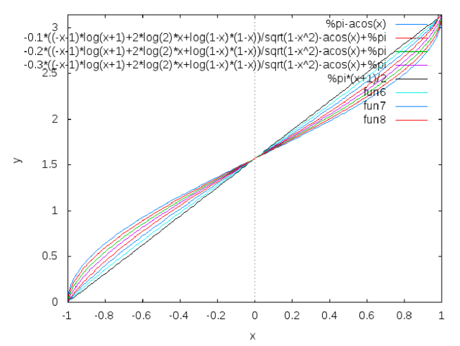
Figure 1.1. An approximate plot of the function $(-1,1)\ni\sigma\mapsto\theta(s,\sigma)$ for some values of $s$. Notice that “the arccosine linearizes” as $s$ goes from $1$ to $0$. The approximate picture is obtained by plotting with Maxima formulas (1.11) (disregarding $o(1-s)$) and (1.12) (disregarding $o(s)$) for some values of $s$. Also, to approximatively plot the function $\Xi$ in (1.13), a high order Taylor expansion of the function $t/\tan t$ at $t=\frac{\pi}{2}$ has been used.

which is also included with the aim of facilitating the interpretation of the mathematical results in (1.11) and (1.12), suggests that this should be the case for every $s\in(0,1)$.

Acknowledgments: It is a pleasure to thank Matteo Cozzi for his very interesting comments on a preliminary version of this paper.

FM was supported by NSF-DMS Grant 1265910 and NSF-DMS FRG Grant 1361122. EV was supported by ERC grant 277749 “E.P.S.I.L.O.N. Elliptic PDE’s and Symmetry of Interfaces and Layers for Odd Nonlinearities” and PRIN grant 201274FYK7 “Critical Point Theory and Perturbative Methods for Nonlinear Differential Equations”.

2. Proof of Theorem 1.1

We start with the following lemma.

Lemma 2.1.

If $\alpha\in\left(0,\frac{\pi}{2}\right)$, then

$$\int_{0}^{\alpha}\left[\int_{0}^{+\infty}\frac{\log\left({r}^{2}+2\,r\,\cos t+1\right)}{{\left({r}^{2}+2\,r\,\cos t+1\right)}^{\frac{3}{2}}}\,r\,dr\right]\,dt=\frac{4(1-\cos\alpha)+2\big{(}\log(\cos\alpha+1)-\log 2\big{)}}{\sin\alpha}\,.$$ (2.1)

Proof.

To show this, given $a$, $r>0$, we let

$$\rho(a,r):=\sqrt{{r}^{2}+2\,a\,r+1}$$

and $$g(a,r):=\frac{2\left(a\,r+1\right)\,\log\rho(a,r)-2\,a\,\rho(a,r)\,\log\left(a+r+\rho(a,r)\right)+2\,a\,r+2}{({a}^{2}-1)\,\rho(a,r)}.$$

By a direct computation, we see that

$$\partial_{r}g(a,r)=\frac{r\,\log\left({r}^{2}+2\,a\,r+1\right)}{{\left({r}^{2}+2\,a\,r+1\right)}^{\frac{3}{2}}}.$$

Also,

$$g(a,0)=\frac{-2a\log(a+1)+2}{a^{2}-1}.$$

In addition, as $r\to+\infty$,

$$\rho(a,r)=r\left(1+\frac{a}{r}+O\left(\frac{1}{r^{2}}\right)\right),$$

and so

$$g(a,r)$$

$$= \frac{1}{({a}^{2}-1)\,r\,\left(1+\frac{a}{r}+O\left(\frac{1}{r^{2}}\right)\right)}\,\left[2\left(a\,r+1\right)\,\log\left(r\left(1+\frac{a}{r}+O\left(\frac{1}{r^{2}}\right)\right)\right)\right.$$

$$\qquad\left.-2\,a\,r\,\left(1+\frac{a}{r}+O\left(\frac{1}{r^{2}}\right)\right)\,\log\left(a+r+r\left(1+\frac{a}{r}+O\left(\frac{1}{r^{2}}\right)\right)\right)+2\,a\,r+2\right]$$

$$= \frac{1}{({a}^{2}-1)\,r\,\left(1+\frac{a}{r}+O\left(\frac{1}{r^{2}}\right)\right)}\,\left[2\left(a\,r+1\right)\,\left[\log r+\log\left(1+\frac{a}{r}+O\left(\frac{1}{r^{2}}\right)\right)\right]\right.$$

$$\qquad\left.-2\,a\,r\,\left(1+\frac{a}{r}+O\left(\frac{1}{r^{2}}\right)\right)\,\left[\log r+\log\left(2+\frac{2a}{r}+O\left(\frac{1}{r^{2}}\right)\right)\right]+2\,a\,r+2\right]$$

$$= \frac{1}{({a}^{2}-1)\,\left(1+o(1)\right)}\,\left[o(1)-2\,a\,\log(2+o(1))+2\,a\right]$$

$$\longrightarrow\frac{2a(1-\log 2)}{a^{2}-1}\qquad{\mbox{ as }}r\to+\infty.$$

As a consequence,

$$\begin{split}&\int_{0}^{+\infty}\frac{\log\left({r}^{2}+2\,a\,r+1\right)}{{\left({r}^{2}+2\,a\,r+1\right)}^{\frac{3}{2}}}\,r\,dr=\int_{0}^{+\infty}\partial_{r}g(a,r)\,dr=g(a,+\infty)-g(a,0)\\ &\qquad\qquad=\frac{2a\big{(}1-\log 2+\log(a+1)\big{)}-2}{a^{2}-1}=:h(a).\end{split}$$ (2.2)

Now, for any $\alpha\in\left(0,\frac{\pi}{2}\right)$, we set

$$H(\alpha):=\frac{4(1-\cos\alpha)+2\big{(}\log(\cos\alpha+1)-\log 2\big{)}}{\sin\alpha}.$$

Notice that

$$\lim_{\alpha\to 0^{+}}H(\alpha)=0.$$

Also, we compute that

$$\partial_{\alpha}H(\alpha)=h(\cos\alpha).$$

Therefore

$$\int_{0}^{\alpha}h(\cos t)\,dt=H(\alpha)-H(0)=\frac{4(1-\cos\alpha)+2\big{(}\log(\cos\alpha+1)-\log 2\big{)}}{\sin\alpha}.$$

Using this and (2.2) with $a:=\cos t$, we obtain (2.1). ∎

Proof of Theorem 1.1.

Since (1.11) and (1.12) (as well as the monotonicity property in $\sigma$ claimed in Theorem 1.1) are invariant for the symmetry

$$\theta(s,-\sigma)=\pi-\theta(s,\sigma),$$

we can assume that $\sigma\in(-1,0)$, and thus (see [MV16]) $\theta(s,\sigma)\in\left(0,\frac{\pi}{2}\right)$. Also, whenever clear from the context, we use the short notation $\theta(s):=\theta(s,\sigma)$. For any $\alpha\in\left(0,\frac{\pi}{2}\right]$ we define the cone of opening $2\alpha$

$$\Gamma_{\alpha}:=\{x=(x_{1},x_{2})\in\mathbb{R}^{2}{\mbox{ s.t. }}x_{2}<-|x|\,\cos\alpha\}.$$

Then, for any $s\in(0,1]$ and $\eta\in[0,+\infty)$, we set

$$I(\eta,\alpha,s):=\int_{\Gamma_{\alpha}}\frac{dz}{|\eta e_{2}-z|^{2+s}}.$$ (2.3)

We know that, see [MV16, Proof of Theorem 1.4, step three],

$$I(1,\alpha,s)=2\,\int_{0}^{\alpha}\left[\int_{0}^{+\infty}\frac{r\,dr}{{\left({r}^{2}+2\,r\,\cos t+1\right)}^{\frac{2+s}{2}}}\right]\,dt$$ (2.4)

and that the optimal angle $\theta=\theta(s)$ in the Young’s law satisfies

$$1+\sigma=\frac{I(1,\theta,s)}{I\left(\sin\theta,\frac{\pi}{2},s\right)}.$$

Also, by scaling (2.3), one sees that

$$I\left(\sin\theta,\frac{\pi}{2},s\right)=\frac{I\left(1,\frac{\pi}{2},s\right)}{(\sin\theta)^{s}}$$

and thus setting

$$f(s,\alpha):=\frac{(\sin\alpha)^{s}\,I(1,\alpha,s)}{I\left(1,\frac{\pi}{2},s\right)}$$

we have

$$f(s,\theta(s))=1+\sigma.$$ (2.5)

Accordingly, recalling that $\theta=\theta(s)$ and differentiating with respect to $s$, we find that

$$\partial_{s}f(s,\theta(s))+\partial_{\alpha}f(s,\theta(s))\,\partial_{s}\theta(s)=0,$$

and so (being, evidently, $\partial_{\alpha}f>0$ for $\alpha\in(0,\pi/2)$)

$$\partial_{s}\theta(s)=-\frac{\partial_{s}f(s,\theta(s))}{\partial_{\alpha}f(s,\theta(s))}\,.$$ (2.6)

Now, to compute $\partial_{s}\theta(1)$ and prove (1.11), we evaluate $\partial_{s}f(1,\theta(1))$ and $\partial_{\alpha}f(1,\theta(1))$ and we substitute these expressions into (2.6) (evaluated at $s=1$). For this, we recall (see [MV16, end of section 4]) that

$$I(1,\alpha,1)=\frac{2\sin\alpha}{1+\cos\alpha}$$ (2.7)

and therefore

$$\partial_{\alpha}I(1,\alpha,1)=\frac{2}{1+\cos\alpha}.$$ (2.8)

In addition,

$$\partial_{\alpha}f(s,\alpha)=\frac{s(\sin\alpha)^{s-1}\cos\alpha\,I(1,\alpha,s)+(\sin\alpha)^{s}\,\partial_{\alpha}I(1,\alpha,s)}{I\left(1,\frac{\pi}{2},s\right)}$$ (2.9)

so that, by (2.8),

$$\partial_{\alpha}f(1,\alpha)=\frac{\frac{2\sin\alpha\,\cos\alpha}{1+\cos\alpha}+\frac{2\sin\alpha}{1+\cos\alpha}}{2}=\sin\alpha\,.$$ (2.10)

On the other hand,

$$\partial_{s}f(s,\alpha)=\frac{(\sin\alpha)^{s}\,\log(\sin\alpha)\,I(1,\alpha,s)}{I\left(1,\frac{\pi}{2},s\right)}+\frac{(\sin\alpha)^{s}\,\partial_{s}I(1,\alpha,s)}{I\left(1,\frac{\pi}{2},s\right)}-\frac{(\sin\alpha)^{s}\,I(1,\alpha,s)\,\partial_{s}I\left(1,\frac{\pi}{2},s\right)}{\left(I\left(1,\frac{\pi}{2},s\right)\right)^{2}},$$ (2.11)

and so, recalling (2.7),

$$\partial_{s}f(1,\alpha)=\frac{\log(\sin\alpha)\sin^{2}\alpha}{1+\cos\alpha}+\frac{\sin\alpha}{2}\,\partial_{s}I(1,\alpha,1)-\frac{\sin^{2}\alpha}{2\,(1+\cos\alpha)}\,\partial_{s}I\left(1,\frac{\pi}{2},1\right).$$ (2.12)

Furthermore, by (2.4),

$$\partial_{s}I(1,\alpha,s)=-\int_{0}^{\alpha}\left[\int_{0}^{+\infty}\frac{\log\left({r}^{2}+2\,r\,\cos t+1\right)r\,dr}{{\left({r}^{2}+2\,r\,\cos t+1\right)}^{\frac{2+s}{2}}}\right]\,dt.$$ (2.13)

Hence, by (2.1),

$$\partial_{s}I(1,\alpha,1)=-\frac{4(1-\cos\alpha)+2\big{(}\log(\cos\alpha+1)-\log 2\big{)}}{\sin\alpha}\,.$$

Now we insert this identity into (2.12) and we conclude that

$$\begin{split}\partial_{s}f(1,\alpha)\,&=\frac{\log(\sin\alpha)\,\sin^{2}\alpha}{\cos\alpha+1}-2(1-\cos\alpha)-\big{(}\log(\cos\alpha+1)-\log 2\big{)}+\frac{(2-\log 2)\sin^{2}\alpha}{\cos\alpha+1}\\ &=(1-\cos\alpha)\big{(}\log(\sin\alpha)-\log 2\big{)}-\log(\cos\alpha+1)+\log 2\,.\end{split}$$ (2.14)

Hence, we insert (2.10) and (2.14) into (2.6) and we find that

$$\partial_{s}\theta(1)=\frac{(\cos\theta(1)-1)\big{(}\log(\sin\theta(1))-\log 2\big{)}+\log(\cos\theta(1)+1)-\log 2}{\sin\theta(1)}\,.$$

Since we have $\cos\theta(1)=-\sigma$ and so $\sin\theta(1)=\sqrt{1-\sigma^{2}}$, we finally conclude that

$$\partial_{s}\theta(1) = \frac{(\sigma+1)\big{(}\log 2-\log(\sqrt{1-\sigma^{2}})\big{)}+\log(1-\sigma)-\log 2}{\sqrt{1-\sigma^{2}}}$$

$$= \frac{2\sigma\log 2+2\log(1-\sigma)-(\sigma+1)\log(1-\sigma^{2})}{2\sqrt{1-\sigma^{2}}}\,.$$

Accordingly, as $s\to 1^{-}$,

$$\theta(s) = \theta(1)+\partial_{s}\theta(1)\,(s-1)+o(1-s)$$

$$= \arccos(-\sigma)-\frac{2\sigma\log 2+(1-\sigma)\log(1-\sigma)-(1+\sigma)\log(1+\sigma)}{2\sqrt{1-\sigma^{2}}}\,(1-s)+o(1-s),$$

which establishes (1.11).

Now we prove (1.12). To this aim, we observe that

$$\left({r}^{2}+2\,r\,\cos t+1\right)^{-\frac{2+s}{2}}=r^{-2-s}+\frac{\kappa}{r^{3+s}},$$ (2.15)

where

$$\kappa=\kappa(r,t,s):=r^{3+s}\left({r}^{2}+2\,r\,\cos t+1\right)^{-\frac{2+s}{2}}-r=r\left(1+\frac{2\,\cos t}{r}+\frac{1}{r^{2}}\right)^{-\frac{2+s}{2}}-r.$$

As a consequence,

$$\int_{1}^{+\infty}\frac{r\,dr}{{\left({r}^{2}+2\,r\,\cos t+1\right)}^{\frac{2+s}{2}}}=\int_{1}^{+\infty}\left[r^{-1-s}+\frac{\kappa}{r^{2+s}}\right]\,dr=\frac{1}{s}+\kappa_{0},$$

where

$$\kappa_{0}=\kappa_{0}(t,s):=\int_{1}^{+\infty}\frac{\kappa}{r^{2+s}}\,dr=\int_{1}^{+\infty}\frac{\left(1+\frac{2\,\cos t}{r}+\frac{1}{r^{2}}\right)^{-\frac{2+s}{2}}-1}{r^{1+s}}\,dr.$$ (2.16)

By a first order expansion, we notice that $\kappa_{0}$ is a function which is bounded uniformly in $t\in\left[0,\frac{\pi}{2}\right]$ and $s\in(0,1)$.

Therefore

$$\int_{0}^{+\infty}\frac{r\,dr}{{\left({r}^{2}+2\,r\,\cos t+1\right)}^{\frac{2+s}{2}}}=\frac{1}{s}+\kappa_{1},$$ (2.17)

where

$$\kappa_{1}=\kappa_{1}(t,s):=\int_{0}^{1}\frac{r\,dr}{{\left({r}^{2}+2\,r\,\cos t+1\right)}^{\frac{2+s}{2}}}+\kappa_{0}(t,s).$$ (2.18)

By construction, we have that $\kappa_{1}$ is bounded uniformly in $t\in\left[0,\frac{\pi}{2}\right]$ and $s\in(0,1)$.

Hence, from (2.4),

$$I(1,\alpha,s)=2\,\int_{0}^{\alpha}\left[\frac{1}{s}+\kappa_{1}\right]\,dt=\frac{2\alpha}{s}+\kappa_{2},$$ (2.19)

where

$$\kappa_{2}=\kappa_{2}(\alpha,s):=2\,\int_{0}^{\alpha}\kappa_{1}\,dt.$$ (2.20)

We remark that $\kappa_{2}$ is bounded uniformly in $\alpha\in\left[0,\frac{\pi}{2}\right]$ and $s\in(0,1)$.

Now, we observe that

$$\liminf_{s\to 0^{+}}\theta(s)>0.$$ (2.21)

Indeed, if, by contradiction, it holds that

$$\lim_{k\to+\infty}\theta(s_{k})=0,$$

for some infinitesimal sequence $s_{k}$, then we deduce from (2.5) that

$$1+\sigma=f(s_{k},\theta(s_{k}))=\lim_{k\to+\infty}\frac{\big{(}\sin(\theta(s_{k})\big{)}^{s_{k}}\,I(1,\theta(s_{k}),s_{k})}{I\left(1,\frac{\pi}{2},s_{k}\right)}\leqslant\lim_{k\to+\infty}\frac{I(1,\theta(s_{k}),s_{k})}{I\left(1,\frac{\pi}{2},s_{k}\right)}.$$

Therefore, by (2.19),

$$0<1+\sigma\leqslant\lim_{k\to+\infty}\frac{\frac{2\theta(s_{k})}{s_{k}}+\kappa_{2}(\theta(s_{k}),s_{k})}{\frac{\pi}{s_{k}}+\kappa_{2}\left(\frac{\pi}{2},s_{k}\right)}=\lim_{k\to+\infty}\frac{2\theta(s_{k})+s_{k}\kappa_{2}(\theta(s_{k}),s_{k})}{\pi+s_{k}\kappa_{2}\left(\frac{\pi}{2},s_{k}\right)}=0,$$

which is a contradiction, thus proving (2.21).

From (2.21), we deduce that

$$\lim_{s\to 0^{+}}\big{(}\sin\theta(s)\big{)}^{s}=1.$$ (2.22)

Therefore, in light of (2.5) and (2.19),

$$1+\sigma=\lim_{s\to 0^{+}}f(s,\theta(s))=\lim_{s\to 0^{+}}\frac{\big{(}\sin(\theta(s)\big{)}^{s}\,I(1,\theta(s),s)}{I\left(1,\frac{\pi}{2},s\right)}$$

$$\qquad=\lim_{s\to 0^{+}}\frac{I(1,\theta(s),s)}{I\left(1,\frac{\pi}{2},s\right)}=\lim_{s\to 0^{+}}\frac{\frac{2\theta(s)}{s}+\kappa_{2}(\theta(s),s)}{\frac{\pi}{s}+\kappa_{2}\left(\frac{\pi}{2},s\right)}$$

$$\qquad=\lim_{s\to 0^{+}}\frac{2\theta(s)+s\kappa_{2}(\theta(s),s)}{\pi+s\kappa_{2}\left(\frac{\pi}{2},s\right)}=\frac{2\lim_{s\to 0^{+}}\theta(s)}{\pi},$$

which proves that

$$\theta(0)=\frac{\pi}{2}(1+\sigma).$$ (2.23)

Now, by (2.16),

$$\kappa_{0}(t,0)=\int_{1}^{+\infty}\frac{\left(1+\frac{2\,\cos t}{r}+\frac{1}{r^{2}}\right)^{-1}-1}{r}\,dr=-\int_{1}^{+\infty}\frac{2\cos t+\frac{1}{r}}{r^{2}+2\,r\cos t+1}\,dr.$$ (2.24)

We also set

$$\varphi(r,t):=\frac{\arctan\left(\frac{\cos t+r}{\sin t}\right)}{\tan t}-\frac{1}{2}\log\frac{r^{2}+2\,r\cos t+1}{r^{2}}$$

and $$\psi(r,t):=\log r-\varphi(r,t)=\frac{1}{2}\log(r^{2}+2\,r\cos t+1)-\frac{\arctan\left(\frac{\cos t+r}{\sin t}\right)}{\tan t}$$

and we compute that

$$\frac{\partial}{\partial r}\varphi(r,t)=\frac{2\cos t+\frac{1}{r}}{r^{2}+2\,r\cos t+1}.$$

From this and (2.24), we conclude that

$$\kappa_{0}(t,0)=\varphi(1,t)-\varphi(+\infty,t)\,.$$ (2.25)

We also remark that

$$\frac{\partial}{\partial r}\psi(r,t)=\frac{\partial}{\partial r}\big{[}\log r-\varphi(r,t)\big{]}=\frac{r}{r^{2}+2\,r\,\cos t+1}$$

and thus

$$\int_{0}^{1}\frac{r\,dr}{{{r}^{2}+2\,r\,\cos t+1}}=\psi(1,t)-\psi(0,t)=-\varphi(1,t)+\frac{\arctan\left(\frac{\cos t}{\sin t}\right)}{\tan t}.$$

Hence, from (2.18) and (2.25),

$$\begin{split}&\kappa_{1}(t,0)=\int_{0}^{1}\frac{r\,dr}{{{r}^{2}+2\,r\,\cos t+1}}+\kappa_{0}(t,0)\\ &\qquad\qquad=\frac{\arctan\left(\frac{\cos t}{\sin t}\right)}{\tan t}-\varphi(+\infty,t)=\frac{\arctan\left(\frac{1}{\tan t}\right)}{\tan t}-\frac{\pi}{2\tan t}.\end{split}$$ (2.26)

Now we point out that, for any $x\in\mathbb{R}$,

$$\frac{1}{2}-\frac{1}{\pi}\arctan\left(\frac{1}{\tan(\pi x)}\right)=\{x\},$$

where $\{\cdot\}$ denotes here the fractional part. As a consequence, for any $t\in\left[0,\frac{\pi}{2}\right]$ (or, more generally, for any $t\in[0,\pi]$) we have

$$\arctan\left(\frac{1}{\tan t}\right)-\frac{\pi}{2}=-\pi\left\{\frac{t}{\pi}\right\}=-t.$$

This and (2.26) say that

$$\kappa_{1}(t,0)=-\frac{t}{\tan t}.$$

Therefore, in the light of (2.20) and recalling the definition in (1.13), we conclude that

$$\kappa_{2}(\alpha,0)=-2\,\int_{0}^{\alpha}\frac{t}{\tan t}\,dt=-2\Xi(\alpha).$$ (2.27)

Now we remark that

$$\log\left({r}^{2}+2\,r\,\cos t+1\right)=\log\left({r}^{2}\left(1+\frac{2\,\cos t}{r}+\frac{1}{r^{2}}\right)\right)$$

$$\qquad\qquad=\log r^{2}+\log\left(1+\frac{2\,\cos t}{r}+\frac{1}{r^{2}}\right)=2\log r+\frac{\chi_{0}}{r},$$

where $\chi_{0}=\chi_{0}(r,t)$ is bounded uniformly in $r\in[1,+\infty)$ and $t\in\left[0,\frac{\pi}{2}\right]$. Then, by (2.15), we obtain

$$\frac{\log\left({r}^{2}+2\,r\,\cos t+1\right)}{{\left({r}^{2}+2\,r\,\cos t+1\right)}^{\frac{2+s}{2}}}\,r=\frac{\left(2\,r\log r+\chi_{0}\right)\left(1+\frac{\kappa}{r}\right)}{r^{2+s}}=\frac{2\,r\log r+2\kappa\log r+\frac{\chi_{0}\kappa}{r}+\chi_{0}}{r^{2+s}}.$$ (2.28)

Furthermore,

$$\frac{\partial}{\partial r}\frac{1+s\,\log r}{s^{2}\,r^{s}}=-\frac{\log r}{r^{1+s}}.$$

This and (2.28) imply that

$$\int_{1}^{+\infty}\frac{\log\left({r}^{2}+2\,r\,\cos t+1\right)}{{\left({r}^{2}+2\,r\,\cos t+1\right)}^{\frac{2+s}{2}}}\,r\,dr=2\int_{1}^{+\infty}\frac{\log r}{r^{1+s}}\,dr+\chi_{1}=\frac{2}{s^{2}}+\chi_{1},$$

with $\chi_{1}=\chi_{1}(t,s)$, which is bounded uniformly in $t\in\left[0,\frac{\pi}{2}\right]$ and $s\in(0,1)$.

Consequently,

$$\int_{0}^{+\infty}\frac{\log\left({r}^{2}+2\,r\,\cos t+1\right)}{{\left({r}^{2}+2\,r\,\cos t+1\right)}^{\frac{2+s}{2}}}\,r\,dr=\frac{2}{s^{2}}+\chi_{2},$$

with $\chi_{2}=\chi_{2}(t,s)$, which is bounded uniformly in $t\in\left[0,\frac{\pi}{2}\right]$ and $s\in(0,1)$. From this identity and (2.13), we obtain

$$\partial_{s}I(1,\alpha,s)=-\int_{0}^{\alpha}\left[\frac{2}{s^{2}}+\chi_{2}\right]\,dt=-\frac{2\alpha}{s^{2}}+\chi_{3},$$

with $\chi_{3}=\chi_{3}(\alpha,s)$ bounded uniformly in $\alpha\in\left[0,\frac{\pi}{2}\right]$ and $s\in(0,1)$.

Using this and (2.19), we have

$$\begin{split}&\frac{(\sin\alpha)^{s}\,\partial_{s}I(1,\alpha,s)}{I\left(1,\frac{\pi}{2},s\right)}-\frac{(\sin\alpha)^{s}\,I(1,\alpha,s)\,\partial_{s}I\left(1,\frac{\pi}{2},s\right)}{\left(I\left(1,\frac{\pi}{2},s\right)\right)^{2}}\\ =\;&\frac{(\sin\alpha)^{s}\,\left(-\frac{2\alpha}{s^{2}}+\chi_{3}\right)}{\frac{\pi}{s}+\bar{\kappa}_{2}}-\frac{(\sin\alpha)^{s}\,\left(\frac{2\alpha}{s}+\kappa_{2}\right)\,\left(-\frac{\pi}{s^{2}}+\chi_{3}\right)}{\left(\frac{\pi}{s}+\bar{\kappa}_{2}\right)^{2}}\\ =\;&\frac{(\sin\alpha)^{s}}{\left(\frac{\pi}{s}+\bar{\kappa}_{2}\right)^{2}}\left[\left(-\frac{2\alpha}{s^{2}}+\chi_{3}\right)\left(\frac{\pi}{s}+\bar{\kappa}_{2}\right)-\left(\frac{2\alpha}{s}+\kappa_{2}\right)\,\left(-\frac{\pi}{s^{2}}+\chi_{3}\right)\right]\\ =\;&\frac{(\sin\alpha)^{s}\,\eta}{\left(\pi+s\bar{\kappa}_{2}\right)^{2}},\end{split}$$ (2.29)

where we used the short notations $\kappa_{2}=\kappa_{2}(\alpha,s)$, $\bar{\kappa}_{2}:=\kappa_{2}\left(\frac{\pi}{2},s\right)$ and

$$\eta=\eta(\alpha,s):=s\chi_{3}\,(\pi-2\alpha+s\bar{\kappa}_{2}-s\kappa_{2})+\pi\kappa_{2}-2\alpha\bar{\kappa}_{2}.$$

We stress that an important simplification occurred in the last step of (2.29).

Notice also that

$$\eta(\alpha,0)=\pi\kappa_{2}(\alpha,0)-2\alpha\kappa_{2}\left(\frac{\pi}{2},0\right).$$ (2.30)

Furthermore, recalling (2.19),

$$\frac{(\sin\alpha)^{s}\,\log(\sin\alpha)\,I(1,\alpha,s)}{I\left(1,\frac{\pi}{2},s\right)}=\frac{(\sin\alpha)^{s}\,\log(\sin\alpha)\,\left(\frac{2\alpha}{s}+\kappa_{2}\right)}{\frac{\pi}{s}+\bar{\kappa}_{2}}=\frac{(\sin\alpha)^{s}\,\log(\sin\alpha)\,\left(2\alpha+s\kappa_{2}\right)}{\pi+s\bar{\kappa}_{2}}.$$

Using this, (2.11) and (2.29), we conclude that

$$\partial_{s}f(s,\alpha)=\frac{(\sin\alpha)^{s}\,\log(\sin\alpha)\,\left(2\alpha+s\kappa_{2}\right)}{\pi+s\bar{\kappa}_{2}}+\frac{(\sin\alpha)^{s}\,\eta}{\left(\pi+s\bar{\kappa}_{2}\right)^{2}}.$$

Thus, recalling also (2.22) and (2.27),

$$\partial_{s}f(0,\theta(0))=\frac{2\theta(0)\,\log\big{(}\sin\theta(0)\big{)}}{\pi}-\frac{2\pi\Xi\big{(}\theta(0)\big{)}-4\theta(0)\,\Xi\left(\frac{\pi}{2}\right)}{\pi^{2}}.$$ (2.31)

Now we observe that, in view of (2.4) and (2.17),

$$\partial_{\alpha}I(1,\alpha,s)=2\,\int_{0}^{+\infty}\frac{r\,dr}{{\left({r}^{2}+2\,r\,\cos\alpha+1\right)}^{\frac{2+s}{2}}}=\frac{2}{s}+\tilde{\kappa}_{1},$$

where $\tilde{\kappa}_{1}=\tilde{\kappa}_{1}(\alpha,s)$ is a function which is bounded uniformly in $\alpha\in\left[0,\frac{\pi}{2}\right]$ and $s\in(0,1)$. Consequently, recalling (2.9) and (2.19),

$$\partial_{\alpha}f(s,\alpha) = \frac{s(\sin\alpha)^{s-1}\cos\alpha\,\left(\frac{2\alpha}{s}+\kappa_{2}\right)+(\sin\alpha)^{s}\,\left(\frac{2}{s}+\tilde{\kappa}_{1}\right)}{\frac{\pi}{s}+\bar{\kappa}_{2}}$$

$$= \frac{s(\sin\alpha)^{s-1}\cos\alpha\,\left({2\alpha}+s\kappa_{2}\right)+(\sin\alpha)^{s}\,\left(2+s\tilde{\kappa}_{1}\right)}{\pi+s\bar{\kappa}_{2}}.$$

Therefore, exploiting (2.22) once again,

$$\partial_{\alpha}f(0,\theta(0))=\frac{2}{\pi}.$$

Making use of this, (2.6) and (2.31), we find

$$\partial_{s}\theta(0)=-\,\theta(0)\,\log\big{(}\sin\theta(0)\big{)}+\frac{\pi\Xi\big{(}\theta(0)\big{)}-2\theta(0)\,\Xi\left(\frac{\pi}{2}\right)}{\pi}.$$

Accordingly, by (2.23),

$$\partial_{s}\theta(0)=-\frac{\pi\,(1+\sigma)}{2}\,\log\left(\cos\frac{\pi\sigma}{2}\right)+\,\Xi\left(\frac{\pi(1+\sigma)}{2}\right)-(1+\sigma)\,\Xi\left(\frac{\pi}{2}\right).$$

From this and (2.23), the desired result in (1.12) plainly follows.

Now we check the monotonicity of the function $\theta(s,\sigma)$ with respect to $\sigma$. For this, we differentiate (2.5) (recall that now $\theta=\theta(s,\sigma)$) and see that

$$f_{\alpha}(s,\theta(s,\sigma))\,\partial_{\sigma}\theta(s,\sigma)=1.$$ (2.32)

Also, from (2.4), we have that $\partial_{\alpha}I(1,\alpha,s)>0$. Accordingly, by (2.9), we obtain that $\partial_{\alpha}f(s,\alpha)>0$. This and (2.32) give that $\partial_{\sigma}\theta(s,\sigma)>0$, as desired. ∎

Appendix A Remarks on the shape of the minimizers

It is interesting to remark that minimizers of capillarity problems with $\sigma=0$, $g=0$, $n=2$ and $\Omega=H=\{x_{2}>0\}$ are not half-balls, differently to what happens in the classical case.

To check this statement, suppose, by contradiction, that $B=HB_{\rho}(0)$ is a critical point (here and in the sequel, for typographical convenience, we use the short notation for intersection of sets $AB:=A\cap B$). Let $x\in H\,\partial B$ and denote by $R$ the reflected half-ball with respect to the tangent line to $\partial B$ at $x$. We observe that $R\subset H$ and $B^{c}\supset H^{c}$. Then, by formula (1.23) in [MV16], the Euler-Lagrange equation at any point $x\in H\,\partial B$ reads as

$$\begin{split}0\,&=\int_{\mathbb{R}^{2}}\frac{1_{B^{c}}(y)-1_{B}(y)}{|x-y|^{2+s}}\,dy-\int_{H^{c}}\frac{dy}{|x-y|^{2+s}}\\ &=\int_{B^{c}H}\frac{dy}{|x-y|^{2+s}}-\int_{B}\frac{dy}{|x-y|^{2+s}}\\ &=\int_{R}\frac{dy}{|x-y|^{2+s}}+\int_{B^{c}R^{c}H}\frac{dy}{|x-y|^{2+s}}-\int_{B}\frac{dy}{|x-y|^{2+s}}\\ &=\int_{B^{c}R^{c}H}\frac{dy}{|x-y|^{2+s}}=:{\mathcal{F}}(x),\end{split}$$ (A.1)

where a cancellation due to the symmetry between $B$ and $R$ was used in the last step of this identity.

Now we evaluate (A.1) at $p=(-\rho,0)$ (see Figure A.1) and at $q=(0,\rho)$ (see Figure A.2), we use some geometric argument exploiting isometric regions of $B^{c}R^{c}H$ and we obtain the desired contradiction.

Figure A.1. Formula (A.1) evaluated at $p=(-\rho,0)$.

Figure A.2. Formula (A.1) evaluated at $q=(0,\rho)$.

To this aim, we observe that, by (A.1),

$${\mathcal{F}}(p)=0={\mathcal{F}}(q).$$ (A.2)

On the other hand, we claim that

$${\mathcal{F}}(p)<{\mathcal{F}}(q).$$ (A.3)

For this, we partition $B^{c}R^{c}H$ into the regions $L$, $M$, $S$, $T$, $W$ and $X$ in Figure A.1 and into the regions $L$, $M$, $S$, $T$, $S^{\prime}$, $T^{\prime}$, $X$, $Y$ and $W$ in Figure A.2.

We observe that the contributions coming from $L$, $M$, $S$, $T$, $X$ and $W$ in Figure A.1 are, by isometry, exactly the same as the ones coming from $L$, $M$, $S$, $T$, $X$ and $W$ in Figure A.2.

Also, Figure A.2 possesses the additional contributions from $S^{\prime}$, $T^{\prime}$ and $Y$ that are not present in Figure A.1. Therefore, the total contributions in Figure A.2 are larger than the ones in Figure A.1, and this proves (A.3).

Then, a contradiction arises by comparing (A.2) and (A.3), thus proving that half-balls are not critical (and, in particular, not minimal).

Appendix B Proof of the asymptotics in (1.3)

.

Up to scaling, we may assume that $\Omega\subseteq B_{1}$. Then, from formula (3.9) in [DFPV13], we have that

$$\lim_{s\to 0^{+}}s\,I_{s}(E,E^{c}\cap\Omega)\leqslant\lim_{s\to 0^{+}}s\,\int_{E}\,dx\,\int_{B_{1}\setminus E}\frac{dy}{|x-y|^{n+s}}=0.$$ (B.1)

Similarly, for any $R\geqslant 1$,

$$\lim_{s\to 0^{+}}s\,\int_{E}\,dx\,\int_{B_{R}\cap\Omega^{c}}\frac{dy}{|x-y|^{n+s}}\leqslant\lim_{s\to 0^{+}}s\,\int_{\Omega}\,dx\,\int_{B_{R}\cap\Omega^{c}}\frac{dy}{|x-y|^{n+s}}=0.$$ (B.2)

Also, from (2.2) in [DFPV13],

$$\alpha(\Omega^{c}):=\lim_{s\to 0^{+}}s\,\int_{\Omega^{c}\cap B_{1}^{c}}\frac{dy}{|y|^{n+s}}=\lim_{s\to 0^{+}}s\,\int_{B_{1}^{c}}\frac{dy}{|y|^{n+s}}=:\bar{c}(n).$$

This and formula (3.8) in [DFPV13] give that

$$0 = \lim_{R\to+\infty}\lim_{s\to 0^{+}}\left|\alpha(\Omega^{c})\,|E|-s\,\int_{E}\,dx\,\int_{\Omega^{c}\cap B_{R}^{c}}\frac{dy}{|x-y|^{n+s}}\right|$$

$$= \lim_{R\to+\infty}\lim_{s\to 0^{+}}\left|\bar{c}(n)\,|E|-s\,\int_{E}\,dx\,\int_{\Omega^{c}\cap B_{R}^{c}}\frac{dy}{|x-y|^{n+s}}\right|.$$

From this and (B.2) we obtain that

$$\lim_{s\to 0^{+}}\left|\bar{c}(n)\,|E|-s\,\int_{E}\,dx\,\int_{\Omega^{c}}\frac{dy}{|x-y|^{n+s}}\right|$$

$$\qquad\leqslant\lim_{R\to+\infty}\lim_{s\to 0^{+}}\left|\bar{c}(n)\,|E|-s\,\int_{E}\,dx\,\int_{\Omega^{c}\cap B_{R}^{c}}\frac{dy}{|x-y|^{n+s}}\right|$$

$$\qquad\qquad+s\,\int_{E}\,dx\,\int_{\Omega^{c}\cap B_{R}}\frac{dy}{|x-y|^{n+s}}=0,$$

that is

$$\lim_{s\to 0^{+}}s\,I_{s}(E,\Omega^{c})=\bar{c}(n)\,|E|.$$

This and (B.1) imply (1.3).

References

• [ADPM11] Luigi Ambrosio, Guido De Philippis, and Luca Martinazzi. Gamma-convergence of nonlocal perimeter functionals. Manuscripta Math., 134(3-4):377–403, 2011. CODEN MSMHB2. ISSN 0025-2611. URL http://dx.doi.org/10.1007/s00229-010-0399-4.
• [BBM01] Jean Bourgain, Haim Brezis, and Petru Mironescu. Another look at sobolev spaces. In in Optimal Control and Partial Differential Equations, pages 439–455, 2001.
• [CRS10] L. Caffarelli, J.-M. Roquejoffre, and O. Savin. Nonlocal minimal surfaces. Comm. Pure Appl. Math., 63(9):1111–1144, 2010. CODEN CPAMA. ISSN 0010-3640. URL http://dx.doi.org/10.1002/cpa.20331.
• [CV11] Luis Caffarelli and Enrico Valdinoci. Uniform estimates and limiting arguments for nonlocal minimal surfaces. Calc. Var. Partial Differential Equations, 41(1-2):203–240, 2011. ISSN 0944-2669. URL http://dx.doi.org.ezproxy.lib.utexas.edu/10.1007/s00526-010-0359-6.
• [CV13] Luis Caffarelli and Enrico Valdinoci. Regularity properties of nonlocal minimal surfaces via limiting arguments. Adv. Math., 248:843–871, 2013. ISSN 0001-8708. URL http://dx.doi.org.pros.lib.unimi.it/10.1016/j.aim.2013.08.007.
• [Dáv02] J. Dávila. On an open question about functions of bounded variation. Calc. Var. Partial Differential Equations, 15(4):519–527, 2002. ISSN 0944-2669. URL http://dx.doi.org/10.1007/s005260100135.
• [DdPW13] Juan Davila, Manuel del Pino, and Juncheng Wei. Nonlocal minimal Lawson cones, 2013. Preprint arXiv:1303.0593.
• [DFPV13] Serena Dipierro, Alessio Figalli, Giampiero Palatucci, and Enrico Valdinoci. Asymptotics of the $s$-perimeter as $s\searrow 0$. Discrete Contin. Dyn. Syst., 33(7):2777–2790, 2013. ISSN 1078-0947. URL http://dx.doi.org.pros.lib.unimi.it/10.3934/dcds.2013.33.2777.
• [DSV15] Serena Dipierro, Ovidiu Savin, and Enrico Valdinoci. Boundary behavior of nonlocal minimal surfaces. ArXiv e-prints, June 2015.
• [DV16] S. Dipierro and E. Valdinoci. Nonlocal minimal surfaces: interior regularity, quantitative estimates and boundary stickiness. ArXiv e-prints, July 2016.
• [Fin86] R. Finn. Equilibrium Capillary Surfaces, volume 284 of Die Grundlehren der mathematischen Wissenschaften. Springer-Verlag New York Inc., New York, 1986.
• [MS02] V. Mazya and T. Shaposhnikova. On the Bourgain, Brezis, and Mironescu theorem concerning limiting embeddings of fractional Sobolev spaces. J. Funct. Anal., 195(2):230–238, 2002. CODEN JFUAAW. ISSN 0022-1236. URL http://dx.doi.org.pros.lib.unimi.it/10.1006/jfan.2002.3955.
• [MV16] F. Maggi and E. Valdinoci. Capillarity problems with nonlocal surface tension energies. ArXiv e-prints, June 2016.
• [XWW16] X. Xu, D. Wang, and X. Wang. An efficient threshold dynamics method for wetting on rough surfaces. ArXiv e-prints, February 2016.