Two-body wave functions and compositeness from scattering amplitudes.
I. General properties with schematic models

Abstract

For a general two-body bound state in quantum mechanics, both in the stable and decaying cases, we establish a way to extract its two-body wave function in momentum space from the scattering amplitude of the constituent two particles. For this purpose, we first show that the two-body wave function of the bound state corresponds to the residue of the off-shell scattering amplitude at the bound state pole. Then, we examine our scheme to extract the two-body wave function from the scattering amplitude in several schematic models. As a result, the two-body wave functions from the Lippmann–Schwinger equation coincides with that from the Schrödinger equation for an energy-independent interaction. Of special interest is that the two-body wave function from the scattering amplitude is automatically scaled; the norm of the two-body wave function, to which we refer as the compositeness, is unity for an energy-independent interaction, while the compositeness deviates from unity for an energy-dependent interaction, which can be interpreted to implement missing channel contributions. We also discuss general properties of the two-body wave function and compositeness for bound states with the schematic models.

I Introduction

The wave function is one of the most fundamental quantities in quantum mechanics, and to determine the wave function is the most important subject in understanding the character of a quantum system. This fact can be seen especially in a bound state of two particles in a quantum system. In the nonrelativistic condition, such a system is governed by the Schrödinger equation, and the wave function of the bound state is evaluated as an eigenfunction of the Hamiltonian in the Schrödinger equation, bringing a discrete eigenvalue, which is nothing but the eigenenergy of the bound state. The wave function of the bound state represents the behavior of the two constituents inside the bound system in coordinate or momentum space. Namely, the squared value of the wave function corresponds to the “probability” of the amplitude of the quantum fluctuation by the constituent two particles in coordinate or momentum space. Moreover, the wave function can be utilized for, e.g., the calculation of the transition amplitude from the bound state to other states and vice versa.

Besides, the properties of the quantum system are reflected also in the scattering amplitude of the two particles, which is the solution of the Lippmann–Schwinger equation. Interestingly, if there exists a bound state in the quantum system, the bound state must be accompanied by a pole in the complex energy plane of the scattering amplitude for the constituent two particles. The pole position coincides with the eigenvalue of the Hamiltonian in the Schrödinger equation associated with the bound state wave function, and hence determining the pole position of the bound state is equivalent to evaluating the discrete eigenvalue of the Hamiltonian.

Then, we can naïvely expect that we may extract properties of the bound state from the scattering amplitude of two constituents, especially from the residue of the scattering amplitude at the pole. In this line, a famous study was done by Weinberg Weinberg:1965zz . In his study, by using the Schrödinger equation and Lippmann–Schwinger equation and taking the weak binding limit of a bound state, he expressed the scattering length and effective range model independently in terms of the so-called field renormalization constant, which equals unity minus norm of the two-body wave function for the bound state. Then, from the experimental values of the scattering length and effective range for the proton–neutron scattering, he concluded that the deuteron is indeed a proton–neutron bound state. An essential point in this discussion is that, since the deuteron pole position exists very close to the lower limit of the physically accessible energy, i.e., the proton–neutron threshold, we can relate the residue of the scattering amplitude at the deuteron pole with the observable threshold parameters in a model independent manner. After several decades from the work by Weinberg, studies on the structure of near threshold bound and resonance states have been recently done in, e.g., Refs. Baru:2003qq ; Hyodo:2013iga ; Hyodo:2014bda ; Hanhart:2014ssa ; Kamiya:2015aea ; Kamiya:2016oao .

In general cases, however, the pole position is not located near the two-body threshold but largely below the threshold or has negatively large imaginary part. In such a case, we have to employ a model to investigate the structure of the bound/resonance state. In this line, a well-known result from decades ago is that, for a given interaction which generates a stable bound state, one can relate the residue of the scattering amplitude at the pole with the wave function of the bound state Gottfried:2003 . The discussion was extended in Ref. Hernandez:1984zzb especially to resonance states, where the authors proved that, with a general energy-independent interaction, a resonance wave function in momentum space can be obtained from the residue of the scattering amplitude of the constituent two particles at the pole position and is correctly normalized as unity. Then, the structure of the bound state from the coupled-channels scattering amplitude is investigated with a separable interaction in Refs. Gamermann:2009uq ; YamagataSekihara:2010pj , where the two-body wave function was found to be proportional to the residue of the scattering amplitude at the resonance pole. Recently, the norm of the two-body wave function, which is called compositeness Hyodo:2011qc ; Hyodo:2013nka , has been extracted from the hadron–hadron scattering amplitude with the separable interaction for candidates of hadronic molecules in, e.g., Refs. Hyodo:2013nka ; Aceti:2012dd ; Sekihara:2012xp ; Xiao:2012vv ; Aceti:2014ala ; Aceti:2014wka ; Nagahiro:2014mba ; Sekihara:2014kya ; Garcia-Recio:2015jsa ; Guo:2016wpy ; Sekihara:2015gvw ; Guo:2015daa .

In the present study, from a more general point of view, we investigate the relation between the wave function of the two-body bound state in momentum space, including the case of an unstable state, and the scattering amplitude of the two particles. Compared to the works in the literature, we further introduce the energy dependence for a general two-body interaction, consider the semirelativistic formulation and the coupled-channels problems, and take into account self-energy effect for an unstable constituent. We show that solving the Lippmann–Schwinger equation at the pole position of the bound state is equivalent to evaluating the two-body wave function of the bound state in momentum space which is automatically scaled. An interesting finding is that the compositeness from the scattering amplitude deviates from unity for energy dependent interactions, which can be interpreted as missing channel contributions. A basic idea of our approach was partly given in Ref. Sekihara:2015gvw , and we extend this to resonances in practical problems, for which we employ the complex scaling method Aoyama:2006 .

This paper is organized as follows. In Sec. II, we formulate the two-body wave functions and compositeness for bound states in general quantum systems in the nonrelativistic and semirelativistic conditions. In the formulation, we show that the two-body wave function of the bound state, both in the stable and decaying cases, appears in the residue of the off-shell scattering amplitude at its pole. Next, in Sec. III, we give numerical calculations of the two-body wave functions and compositeness in several schematic models for bound states. Section IV is devoted to the summary of this study. This is the first paper of a series for the two-body wave function and compositeness in general quantum systems; our scheme constructed here will be applied to the physical $N^{\ast}$ and $\Delta^{\ast}$ resonances in a precise scattering amplitude Sekihara:2016 .

II Formulation

In this section, we formulate the two-body wave function for a bound state, regardless of whether the bound state is stable or not. For this purpose, we first give a setup of the quantum system in Sec. II.1. Next, we formulate the Schrödinger equation for the bound state in Sec. II.2. In this section we also define the so-called compositeness as the norm of the two-body wave function for the bound state. Then, in Sec. II.3, we clarify how the two-body wave function appears in the scattering amplitude, which is a solution of the Lippmann–Schwinger equation, and propose a way to extract the two-body wave function for the bound state from the scattering amplitude. The model dependence of the compositeness is discussed in Sec. II.4. Finally, in order to investigate numerically the structure of a resonance state, we show our formulae of the wave function, compositeness, and so on, in the complex scaling method in Sec. II.5.

II.1 Setup of the system

In this paper we consider a two-body to two-body coupled-channels scattering system. The system is governed by the full Hamiltonian $\hat{H}$, which can be decomposed into the free Hamiltonian $\hat{H}_{0}$ and the interaction part $\hat{V}$:

$$\hat{H}=\hat{H}_{0}+\hat{V}(E).$$ (1)

Here, we assume that we have only the two-body states in the practical model space, i.e., we do not treat one-body bare states nor states composed of more than two particles acted by $\hat{H}$, $\hat{H}_{0}$, and $\hat{V}$. In addition, we assume that the scattering process with the interaction $\hat{V}$ is time-reversal invariant and, for the later applications, we allow the interaction to depend intrinsically on the energy of the system $E$, which corresponds to the eigenenergy of the full Hamiltonian. We neglect the spin of the scattering particles for simplicity.

As an eigenstate of the free Hamiltonian $\hat{H}_{0}$, we introduce the $j$th channel two-body scattering state with relative three-momentum $\bm{q}$ as $|\bm{q}_{j}\rangle$:

$$\hat{H}_{0}|\bm{q}_{j}\rangle=\mathcal{E}_{j}(q)|\bm{q}_{j}\rangle,\quad\langle\bm{q}_{j}|\hat{H}_{0}=\mathcal{E}_{j}(q)\langle\bm{q}_{j}|,$$ (2)

where $q\equiv|\bm{q}|$ is the magnitude of the momentum $\bm{q}$. For the eigenenergy $\mathcal{E}_{j}(q)$, we employ two options. One is the nonrelativistic form containing the threshold energy

$$\mathcal{E}_{j}(q)\equiv m_{j}+M_{j}+\frac{q^{2}}{2\mu_{j}},\quad\mu_{j}\equiv\frac{m_{j}M_{j}}{m_{j}+M_{j}},$$ (3)

and the other is the semirelativistic form

$$\mathcal{E}_{j}(q)\equiv\sqrt{q^{2}+m_{j}^{2}}+\sqrt{q^{2}+M_{j}^{2}}.$$ (4)

Here, $m_{j}$ and $M_{j}$ are masses of scattering particles in the channel $j$ and $\mu_{j}$ is the reduced mass for them. In the present study, the scattering state is normalized as

$$\langle\bm{q}_{j}^{\prime}|\bm{q}_{k}\rangle=(2\pi)^{3}\delta_{jk}\delta(\bm{q}^{\prime}-\bm{q}).$$ (5)

In terms of the eigenstates $|\bm{q}_{j}\rangle$, the free Hamiltonian can be expressed as

$$\hat{H}_{0}=\sum_{j}\int\frac{d^{3}q}{(2\pi)^{3}}\mathcal{E}_{j}(q)|\bm{q}_{j}\rangle\langle\bm{q}_{j}|.$$ (6)

For the interaction $\hat{V}$, on the other hand, we employ a general form in the following coupled-channels expression with the two-body scattering states in coordinate space $|\bm{r}_{j}\rangle$:

$$\langle\bm{r}_{j}^{\prime}|\hat{V}(E)|\bm{r}_{k}\rangle=V_{jk}(E;\,\bm{r}^{\prime},\,\bm{r}).$$ (7)

Here, $\bm{r}$ is the relative distance between two particles in the considering channel, $r$ is its magnitude, $r\equiv|\bm{r}|$, and the $j$th channel scattering state $|\bm{r}_{j}\rangle$ is normalized as

$$\langle\bm{r}_{j}^{\prime}|\bm{r}_{k}\rangle=\delta_{jk}\delta(\bm{r}^{\prime}-\bm{r}).$$ (8)

The interaction term in coordinate space $V_{jk}(E;\,\bm{r}^{\prime},\,\bm{r})$ may, as we have mentioned, depend intrinsically on the energy of the system $E$. Since we assume the time-reversal invariance of the scattering process, the interaction term satisfies a relation

$$V_{jk}(E;\,\bm{r}^{\prime},\,\bm{r})=V_{kj}(E;\,\bm{r},\,\bm{r}^{\prime}),$$ (9)

with an appropriate choice of phases of the states.

We also consider the matrix element of the interaction with the scattering states in momentum space:

$$\langle\bm{q}_{j}^{\prime}|\hat{V}(E)|\bm{q}_{k}\rangle=\tilde{V}_{jk}(E;\,\bm{q}^{\prime},\,\bm{q}).$$ (10)

This is related to the matrix element in coordinate space (7) via the Fourier transformation as

$$\tilde{V}_{jk}(E;\,\bm{q}^{\prime},\,\bm{q}) =\int d^{3}r^{\prime}\int d^{3}r\,\langle\bm{q}_{j}^{\prime}|\bm{r}_{j}^{\prime}\rangle\langle\bm{r}_{j}^{\prime}|\hat{V}(E)|\bm{r}_{k}\rangle\langle\bm{r}_{k}|\bm{q}_{k}\rangle$$

$$=\int d^{3}r^{\prime}\int d^{3}r\,V_{jk}(E;\,\bm{r}^{\prime},\,\bm{r})e^{-i\bm{q}^{\prime}\cdot\bm{r}^{\prime}+i\bm{q}\cdot\bm{r}},$$ (11)

where we have used $\langle\bm{q}_{j}|\bm{r}_{k}\rangle=\delta_{jk}e^{-i\bm{q}\cdot\bm{r}}$. We note that the time-reversal invariance of the scattering process brings a relation

$$\hat{V}_{jk}(E;\,\bm{q}^{\prime},\,\bm{q})=\hat{V}_{kj}(E;\,\bm{q},\,\bm{q}^{\prime}),$$ (12)

with an appropriate choice of phases of the states.

II.2 Schrödinger equation

Let us now suppose that the full Hamiltonian has a discrete eigenstate $|\psi_{LM}\rangle$ in the partial wave $L$ with its azimuthal component $M$, in addition to the ordinary scattering states. We formulate the Schrödinger equation and wave function for this discrete eigenstate. If its eigenvalue $E_{\rm pole}$ is a real number, we can treat the $|\psi_{LM}\rangle$ state as a usual stable bound state. On the other hand, if $E_{\rm pole}$ has an imaginary part, the eigenstate $|\psi_{LM}\rangle$ is a resonance state; $\text{Re}\,E_{\rm pole}$ and $-2\,\text{Im}\,E_{\rm pole}$ are the mass and width of the resonance state, respectively. Since we treat both bound and resonance states on the same footing in the following discussions, we formulate the Schrödinger equation and wave function in a manner applicable to both cases. In any case, the state $|\psi_{LM}\rangle$ is a solution of the Schrödinger equation

$$\hat{H}|\psi_{LM}\rangle=\left[\hat{H}_{0}+\hat{V}(E_{\rm pole})\right]|\psi_{LM}\rangle=E_{\rm pole}|\psi_{LM}\rangle.$$ (13)

Then, to establish the normalization of the resonance state, we should employ the Gamow vector Hernandez:1984zzb ; Gamow:1928zz ; Hokkyo:1965zz ; Berggren:1968zz ; Romo:1968zz , where we take $\langle\tilde{\psi}_{LM}|\equiv\langle\psi_{LM}^{\ast}|$ instead of $\langle\psi_{LM}|$ for the bra vector of the resonance. In this notation, we can normalize the resonance wave function in the following manner:

$$\langle\tilde{\psi}_{LM^{\prime}}|\psi_{LM}\rangle=\delta_{M^{\prime}M}.$$ (14)

The Schrödinger equation for the resonance bra state is expressed with the same eigenenergy as

$$\langle\tilde{\psi}_{LM}|\hat{H}=\langle\tilde{\psi}_{LM}|\left[\hat{H}_{0}+\hat{V}(E_{\rm pole})\right]=\langle\tilde{\psi}_{LM}|E_{\rm pole}.$$ (15)

From the Schrödinger equation in the operator form (13), we can formulate the usual Schrödinger equation with the c-number wave function. Since in this study we formulate the Schrödinger equation in momentum space and solve it, we employ the $j$th channel wave function in momentum space $\tilde{\psi}_{j}(\bm{q})\equiv\langle\bm{q}_{j}|\psi_{LM}\rangle$. By using the expressions of $\hat{H}_{0}$ and $\hat{V}$ in Eqs. (6) and (10), we can express the Schrödinger equation (13) as

$$\mathcal{E}_{j}(q)\tilde{\psi}_{j}(\bm{q})+\sum_{k}\int\frac{d^{3}q^{\prime}}{(2\pi)^{3}}\tilde{V}_{jk}(E_{\rm pole};\,\bm{q},\,\bm{q}^{\prime})\tilde{\psi}_{k}(\bm{q}^{\prime})$$

$$=E_{\rm pole}\tilde{\psi}_{j}(\bm{q}),$$ (16)

where we have inserted a relation

$$\mbox{1}\mbox{l}_{\rm model}=\sum_{k}\int\frac{d^{3}q^{\prime}}{(2\pi)^{3}}|\bm{q}_{k}^{\prime}\rangle\langle\bm{q}_{k}^{\prime}|,$$ (17)

which is valid in the practical model space, between $\hat{V}$ and $|\psi_{LM}\rangle$. This Schrödinger equation can be simplified with the partial wave decomposition. Namely, on the one hand, the interaction term can be decomposed as

$$\tilde{V}_{jk}(E;\,\bm{q}^{\prime},\,\bm{q})=\sum_{L=0}^{\infty}(2L+1)V_{L,jk}(E;\,q^{\prime},\,q)P_{L}(\hat{q}^{\prime}\cdot\hat{q}),$$ (18)

with $\hat{q}\equiv\bm{q}/q$ being the direction of the vector $\bm{q}$, and each partial wave component can be calculated as

$$V_{L,jk}(E;\,q^{\prime},\,q)=\frac{1}{2}\int_{-1}^{1}d(\hat{q}^{\prime}\cdot\hat{q})P_{L}(\hat{q}^{\prime}\cdot\hat{q})\tilde{V}_{jk}(E;\,\bm{q}^{\prime},\,\bm{q}),$$ (19)

thanks to the relation for the Legendre polynomials $P_{L}(x)$

$$\int_{-1}^{1}dxP_{L}(x)P_{L^{\prime}}(x)=\frac{2}{2L+1}\delta_{LL^{\prime}}.$$ (20)

On the other hand, the wave function $\tilde{\psi}_{j}(\bm{q})$ consists of the radial part $R_{j}(q)$ and the spherical harmonics $Y_{LM}(\hat{q})$ as

$$\tilde{\psi}_{j}(\bm{q})=R_{j}(q)Y_{LM}(\hat{q}).$$ (21)

We fix the normalization of the spherical harmonics $Y_{LM}(\hat{q})$ as

$$\int d\Omega_{\bm{q}}Y_{LM}(\hat{q})Y_{L^{\prime}M^{\prime}}^{\ast}(\hat{q})=4\pi\delta_{LL^{\prime}}\delta_{MM^{\prime}},$$ (22)

with the solid angle $\Omega_{\bm{q}}$ for $\bm{q}$. By using the above expressions in the partial wave decomposition, we can rewrite the Schrödinger equation (16) as

$$\mathcal{E}_{j}(q)R_{j}(q)+\sum_{k}\int_{0}^{\infty}\frac{dq^{\prime}}{2\pi^{2}}q^{\prime 2}V_{L,jk}(E_{\rm pole};\,q,\,q^{\prime})R_{k}(q^{\prime})$$

$$=E_{\rm pole}R_{j}(q),$$ (23)

where we have used the relation in Eq. (22) and

$$P_{L}(\hat{q}^{\prime}\cdot\hat{q})=\frac{1}{2L+1}\sum_{M=-L}^{L}Y_{LM}(\hat{q}^{\prime})Y_{LM}^{\ast}(\hat{q}).$$ (24)

The Schrödinger equation (23) is the final form to evaluate the radial part of the two-body wave function $R_{j}(q)$ for stable bound states. For resonance states, we employ the complex scaling method, which is explained in Sec. II.5. We note that we solve the integral equation (23) numerically by discretizing the momentum and replacing the integral with respect to the momentum with a summation.

Before going to the formulation of the Lippmann–Schwinger equation, we here comment on the norm of the two-body wave function for the resonance state. Namely, while the wave function in momentum space can be written as in Eq. (21) from the ket state $|\psi_{LM}\rangle$, the two-body wave function from the bra state $\langle\tilde{\psi}_{LM}|$, $\langle\tilde{\psi}_{LM}|\bm{q}_{j}\rangle$, can be evaluated as

$$\langle\tilde{\psi}_{LM}|\bm{q}_{j}\rangle=\langle\psi_{LM}^{\ast}|\bm{q}_{j}\rangle=R_{j}(q)Y_{LM}^{\ast}(\hat{q}).$$ (25)

Here we emphasize that, while we take the complex conjugate for the spherical harmonics, we do not take for the radial part. This is because, while the spherical part can be calculated and normalized in a usual sense, the radial part should be treated so as to remove the divergence of the wave function at $r\to\infty$ when we calculate the norm (see discussions in Refs. Hernandez:1984zzb ; Hyodo:2013nka ; Hokkyo:1965zz ; Berggren:1968zz ; Romo:1968zz ). From the above wave function, we can calculate the norm with respect to the $j$th channel two-body wave function, $X_{j}$, in the following manner:

$$X_{j}\equiv\int\frac{d^{3}q}{(2\pi)^{3}}\langle\tilde{\psi}_{LM}|\bm{q}_{j}\rangle\langle\bm{q}_{j}|\psi_{LM}\rangle=\int_{0}^{\infty}dq\,\text{P}_{j}(q),$$ (26)

where we have introduced a density distribution $\text{P}_{j}(q)$:

$$\text{P}_{j}(q)\equiv\frac{q^{2}}{2\pi^{2}}\left[R_{j}(q)\right]^{2}.$$ (27)

The quantity $X_{j}$ is referred to as the compositeness. We note that the compositeness $X_{j}$ as well as the wave function $\tilde{\psi}_{j}(\bm{q})$ is not observable and hence in general a model dependent quantity (see the discussion in Sec. II.4). As we can see from the construction, for the resonance state, the compositeness $X_{j}$ is given by the complex number squared of the radial part $R_{j}(q)$ rather than by the absolute value squared, which is essential to normalize the resonance wave function. Therefore, in general the compositeness becomes complex for resonance states.

We also note that the sum of the norm $X_{j}$ should be unity if there is no missing (or implicit) channels, which would be an eigenstate of the free Hamiltonian, to describe the bound state. However, in actual calculations we may have contributions from missing channels, which can be implemented into the interaction and be origin of the intrinsic energy dependence of the interaction. In such a case, denoting the missing channels representatively as $|\psi_{0}\rangle$, we can decompose unity in terms of the eigenstates of the free Hamiltonian:

$$\mbox{1}\mbox{l}=|\psi_{0}\rangle\langle\psi_{0}|+\sum_{j}\int\frac{d^{3}q}{(2\pi)^{3}}|\bm{q}_{j}\rangle\langle\bm{q}_{j}|,$$ (28)

instead of Eq. (17). Therefore, introducing the missing channel contribution $Z$ defined as

$$Z\equiv\langle\tilde{\psi}_{LM}|\psi_{0}\rangle\langle\psi_{0}|\psi_{LM}\rangle,$$ (29)

which is a model dependent quantity and becomes complex for resonance states as well, we can express the normalization of the wave function $|\psi_{LM}\rangle$ as

$$\langle\tilde{\psi}_{LM}|\psi_{LM}\rangle=Z+\sum_{j}X_{j}=1.$$ (30)

Thus, in contrast to the naïve manner in quantum mechanics, in the present study we do not make the sum of the compositeness $X_{j}$ coincide with unity by hand. Instead, as we will discuss in Sec. II.3, the value of the norm, $X_{j}$, is automatically fixed without any artificial factor when we calculate the residue of the scattering amplitude.

II.3 Lippmann–Schwinger equation

In this subsection we consider the same problem as in the previous subsection with the scattering amplitude. In particular, we show how we can extract the two-body wave function of the bound state from the scattering amplitude. Although the relation between the bound-state wave function and the residue of the scattering amplitude at the pole position is already discussed in the literature, in this study we treat a more general case with an energy dependent interaction in a coupled-channels problem. We note that some of the formulation presented here is already given in Ref. Sekihara:2015gvw , but for completeness we give it in detail.

In general, the scattering amplitude can be formally obtained with the Lippmann–Schwinger equation in an operator form:

$$\hat{T}(E)= \hat{V}(E)+\hat{V}(E)\frac{1}{E-\hat{H}_{0}}\hat{T}(E)$$

$$= \hat{V}(E)+\hat{V}(E)\frac{1}{E-\hat{H}}\hat{V}(E),$$ (31)

with the $T$-matrix operator $\hat{T}$, the free Hamiltonian $\hat{H}_{0}$, and the full Hamiltonian $\hat{H}\equiv\hat{H}_{0}+\hat{V}(E)$. We use the same $\hat{H}$, $\hat{H}_{0}$ and $\hat{V}$ as in the previous subsection. From the $T$-matrix operator $\hat{T}$, we can evaluate scattering amplitude of the $k(\bm{q})\to j(\bm{q}^{\prime})$ scattering, where $\bm{q}^{(\prime)}$ is the relative three-momentum in the initial (final) state, as

$$T_{jk}(E;\,\bm{q}^{\prime},\,\bm{q})\equiv\langle\bm{q}_{j}^{\prime}|\hat{T}(E)|\bm{q}_{k}\rangle.$$ (32)

The scattering state $|\bm{q}_{j}\rangle$ is again the same as in the previous subsection. Due to the time-reversal invariance, the scattering amplitude satisfies

$$T_{jk}(E;\,\bm{q}^{\prime},\,\bm{q})=T_{kj}(E;\,\bm{q},\,\bm{q}^{\prime}),$$ (33)

with an appropriate choice of phases of the states. The scattering amplitude $T_{jk}(E;\,\bm{q}^{\prime},\,\bm{q})$ is a solution of the Lippmann–Schwinger equation in the following form:

$$T_{jk}(E;\,\bm{q}^{\prime},\,\bm{q})=\tilde{V}_{jk}(E;\,\bm{q}^{\prime},\,\bm{q})$$

$$+\sum_{l}\int\frac{d^{3}k}{(2\pi)^{3}}\frac{\tilde{V}_{jl}(E;\,\bm{q}^{\prime},\,\bm{k})T_{lk}(E;\,\bm{k},\,\bm{q})}{E-\mathcal{E}_{l}(k)},$$ (34)

where the interaction term $\tilde{V}_{jk}$ has been introduced in Eq. (10).

Next, let us decompose the scattering amplitude into partial wave amplitudes, as in Eq. (18):

$$T_{jk}(E;\,\bm{q}^{\prime},\,\bm{q})=\sum_{L=0}^{\infty}(2L+1)T_{L,jk}(E;\,q^{\prime},\,q)P_{L}(\hat{q}^{\prime}\cdot\hat{q}),$$ (35)

$$T_{L,jk}(E;\,q^{\prime},\,q)=\frac{1}{2}\int_{-1}^{1}d(\hat{q}^{\prime}\cdot\hat{q})P_{L}(\hat{q}^{\prime}\cdot\hat{q})T_{jk}(E;\,\bm{q}^{\prime},\,\bm{q}).$$ (36)

Since the Legendre polynomials satisfy the following relation

$$\int d\Omega_{\bm{k}}P_{L}(\hat{q}^{\prime}\cdot\hat{k})P_{L^{\prime}}(\hat{k}\cdot\hat{q})=\frac{4\pi}{2L+1}\delta_{LL^{\prime}}P_{L}(\hat{q}^{\prime}\cdot\hat{q}),$$ (37)

we can rewrite the Lippmann–Schwinger equation (34) as

$$T_{L,jk}(E;\,q^{\prime},\,q)=V_{L,jk}(E;\,q^{\prime},\,q)$$

$$+\sum_{l}\int_{0}^{\infty}\frac{dk}{2\pi^{2}}k^{2}\frac{V_{L,jl}(E;\,q^{\prime},\,k)T_{L,lk}(E;\,k,\,q)}{E-\mathcal{E}_{l}(k)}.$$ (38)

This is the final form of the scattering amplitude to be solved for stable bound states. For resonance states we employ the complex scaling method explained in Sec. II.5 to calculate the scattering amplitude. In the numerical calculations of the integral equation (38), we discretize the momentum so as to replace the integral with a summation.

Here we comment on the relation between the energy $E$ and momenta $q$ and $q^{\prime}$. In the physical scattering, the initial and final states should be on their mass shell and their energy should be fixed as $E=\mathcal{E}_{j}(q^{\prime})=\mathcal{E}_{k}(q)$. We call the scattering amplitude in this condition as the on-shell amplitude. An important feature is that, for open channels, the on-shell scattering amplitude is in general observable and can be determined model independently in a partial wave analysis. The on-shell scattering amplitude in each partial wave satisfies the optical theorem from the unitarity of the $S$-matrix, and in our formulation its expression is:

$$\text{Im}\,T_{L,jj}(E)^{\text{on-shell}}=-\sum_{k}\frac{\rho_{k}(E)}{2}\left|T_{L,jk}(E)^{\text{on-shell}}\right|^{2},$$ (39)

where the sum runs over the open channels and $\rho_{j}(E)$ is the phase space in channel $j$, whose expression is

$$\rho_{j}(E)\equiv\frac{\mu_{j}k_{j}(E)}{\pi},\quad k_{j}(E)\equiv\sqrt{2\mu_{j}(E-m_{j}-M_{j})},$$ (40)

for the nonrelativistic case (3), and

$$\rho_{j}(E)\equiv\sqrt{k_{j}(E)^{2}+m_{j}^{2}}\sqrt{k_{j}(E)^{2}+M_{j}^{2}}\frac{k_{j}(E)}{\pi E},$$ (41)

$$k_{j}(E)\equiv\frac{\lambda^{1/2}(E^{2},\,m_{j}^{2},\,M_{j}^{2})}{2E},$$ (42)

for the semirelativistic case (4) with the Källen function $\lambda(x,\,y,\,z)=x^{2}+y^{2}+z^{2}-2xy-2yz-2zx$.

Furthermore, one can perform the analytic continuation of the on-shell amplitude to the complex energy and to the pole position for the bound state, keeping the relation $E=\mathcal{E}_{j}(q^{\prime})=\mathcal{E}_{k}(q)$ with complex momenta $q$ and $q^{\prime}$. Therefore, the pole position $E_{\rm pole}$ and residue of the on-shell amplitude at this pole are in principle determined only with the experimental quantities in a model independent manner.

However, in contrast to the on-shell amplitude, we can mathematically treat the scattering amplitude $T_{L,jk}(E;\,q^{\prime},\,q)$ as a function of three independent variables $E$, $q^{\prime}$, and $q$ as an off-shell amplitude. In particular, we can perform the analytic continuation of the scattering amplitude by taking complex value of the energy $E$ but keeping the momenta $q$ and $q^{\prime}$ real and positive, with which the relation $E=\mathcal{E}_{j}(q^{\prime})=\mathcal{E}_{k}(q)$ is no longer satisfied. This condition of the complex energy $E$ but real and positive momenta $q$ and $q^{\prime}$ will be essential to extract the wave function from the scattering amplitude at the pole position of the bound state in the complex energy plane.

We now explain the way to extract the two-body wave function and compositeness from the off-shell scattering amplitude obtained by the analytic continuation for the energy. The key is the factor $1/(E-\hat{H})$ in the Lippmann–Schwinger equation (31). We start with the fact that the off-shell scattering amplitude as well as the on-shell one has the bound state pole at $E=E_{\rm pole}$. Actually, near the pole, the off-shell scattering amplitude is dominated by the pole term in the expansion by the eigenstates of the full Hamiltonian, and hence we have

$$\hat{T}(E)\approx\sum_{M=-L}^{L}\hat{V}(E_{\rm pole})|\psi_{LM}\rangle\frac{1}{E-E_{\rm pole}}\langle\tilde{\psi}_{LM}|\hat{V}(E_{\rm pole}),$$ (43)

where we have summed up the possible azimuthal component $M$. In this expression, the operator $|\psi_{LM}\rangle\langle\tilde{\psi}_{LM}|$ coincides with a projector of rank $1$ attached to the resonance pole in Ref. Guo:2015daa . This fact indicates the proper normalization of the bound-state wave function $\langle\tilde{\psi}_{LM}|\psi_{LM}\rangle=1$. Then, it is important that the wave function $|\psi_{LM}\rangle$ appears in the residue of the scattering amplitude at the pole. Evaluating the matrix element of this $T$-matrix operator, we obtain

$$T_{jk}(E;\,\bm{q}^{\prime},\,\bm{q})$$

$$\approx\sum_{M=-L}^{L}\frac{\langle\bm{q}_{j}^{\prime}|\hat{V}(E_{\rm pole})|\psi_{LM}\rangle\langle\tilde{\psi}_{LM}|\hat{V}(E_{\rm pole})|\bm{q}_{k}\rangle}{E-E_{\rm pole}}.$$ (45)

The matrix elements in the numerator of the above expression, $\langle\bm{q}_{j}^{\prime}|\hat{V}(E_{\rm pole})|\psi_{LM}\rangle$ and $\langle\tilde{\psi}_{LM}|\hat{V}(E_{\rm pole})|\bm{q}_{k}\rangle$, can be calculated as follows. By using the Schrödinger equation (13), the former matrix element is calculated as

$$\langle\bm{q}_{j}|\hat{V}(E_{\rm pole})|\psi_{LM}\rangle= \langle\bm{q}_{j}|\left(\hat{H}-\hat{H}_{0}\right)|\psi_{LM}\rangle$$

$$= \left[E_{\rm pole}-\mathcal{E}_{j}(q)\right]\langle\bm{q}_{j}|\psi_{LM}\rangle,$$ (46)

and from Eq. (21) we obtain

$$\langle\bm{q}_{j}|\hat{V}(E_{\rm pole})|\psi_{LM}\rangle=\gamma_{j}(q)Y_{LM}(\hat{q}),$$ (47)

where we have defined $\gamma_{j}(q)$ as

$$\gamma_{j}(q)\equiv\left[E_{\rm pole}-\mathcal{E}_{j}(q)\right]R_{j}(q).$$ (48)

In a similar manner we can calculate the latter matrix element as

$$\langle\tilde{\psi}_{LM}|\hat{V}(E_{\rm pole})|\bm{q}_{j}\rangle=\gamma_{j}(q)Y_{LM}^{\ast}(\hat{q}).$$ (49)

Therefore, by using the above matrix elements, we can rewrite the scattering amplitude near the pole as

$$T_{jk}(E;\,\bm{q}^{\prime},\,\bm{q}) \approx\frac{\gamma_{j}(q^{\prime})\gamma_{k}(q)}{E-E_{\rm pole}}\sum_{M=-L}^{L}Y_{LM}(\hat{q}^{\prime})Y_{LM}^{\ast}(\hat{q})$$

$$=(2L+1)\frac{\gamma_{j}(q^{\prime})\gamma_{k}(q)}{E-E_{\rm pole}}P_{L}(\hat{q}^{\prime}\cdot\hat{q}),$$ (50)

where we have used the formula in Eq. (24). Since the amplitude in Eq. (50) is nothing but the $L$-wave component, we can show that indeed the $L$-wave partial wave amplitude contains the pole:

$$T_{L,jk}(E;\,q^{\prime},\,q)=\frac{\gamma_{j}(q^{\prime})\gamma_{k}(q)}{E-E_{\rm pole}}+(\text{regular at }E=E_{\rm pole}).$$ (51)

Then, interestingly, the residue of the partial wave amplitude $\gamma_{j}(q)$ contains information on the two-body wave function as in Eq. (48). Actually, we can calculate the $j$th channel compositeness, $X_{j}$, by using the residue $\gamma_{j}(q)$ as

$$X_{j}=\int_{0}^{\infty}dq\,\text{P}_{j}(q),\quad\text{P}_{j}(q)\equiv\frac{q^{2}}{2\pi^{2}}\left[\frac{\gamma_{j}(q)}{E_{\rm pole}-\mathcal{E}_{j}(q)}\right]^{2}.$$ (52)

This is the formula to evaluate the $j$th channel compositeness $X_{j}$ from the residue of the partial wave amplitude $T_{L}$ at the pole. The residue $\gamma_{j}(q)$ is extracted as a function of the real and positive momentum $q$ from the off-shell amplitude with complex energy $E\to E_{\rm pole}$.

We emphasize that the scattering amplitude, and hence its residue $\gamma_{j}(q)$, is obtained from the Lippmann–Schwinger equation without introducing any extra factor to scale the value of the compositeness $X_{j}$, since the Lippmann–Schwinger equation is an inhomogeneous integral equation. This means that the value of the compositeness in Eq. (52) as well as that of the two-body wave function is automatically fixed without any scaling factor when we calculate it from the residue of the scattering amplitude. In other words, the compositeness from the scattering amplitude is uniquely determined once we fix the model space, form of the kinetic energy $\mathcal{E}_{j}(q)$, and interaction.

The fact that the value of the compositeness in Eq. (52) is automatically fixed leads to the question on the normalization of the compositeness. Actually, a single-channel problem with an energy-independent interaction in a general form was discussed in Ref. Hernandez:1984zzb and the authors found that the norm of the two-body wave function from the scattering amplitude is exactly unity in this case. However, in general the sum of the compositeness from the scattering amplitude may deviate from unity. Therefore, we can define the rest part of the normalization of the total wave function (14) $Z$ as

$$Z\equiv 1-\sum_{j}X_{j}.$$ (53)

Since the compositeness $X_{j}$ is defined as the norm of the two-body wave function, $Z$ can be interpreted as the missing-channel contribution. In Sec. III we will see that the missing-channel contribution $Z$ is exactly zero for the energy-independent interaction, but $Z$ becomes nonzero if we switch on the energy dependence of the interaction.

Finally we comment on the probabilistic interpretation of the compositeness for resonances. As we have discussed, for resonances the compositeness from each channel is in general complex. This means that, strictly speaking, we cannot interpret them as the probability to find each channel component inside the resonance state. In order to cure this point, we would like to introduce quantities $\tilde{X}_{j}$ and $\tilde{Z}$ by following the discussion in Ref. Sekihara:2015gvw as

$$\tilde{X}_{j}\equiv\frac{|X_{j}|}{1+U},\quad\tilde{Z}\equiv\frac{|Z|}{1+U},$$ (54)

with

$$U\equiv\sum_{j}|X_{j}|+|Z|-1.$$ (55)

The quantities $\tilde{X}_{j}$ and $\tilde{Z}$ are real, bound in the range $[0,\,1]$, and automatically satisfy the sum rule:

$$\sum_{j}\tilde{X}_{j}+\tilde{Z}=1.$$ (56)

The quantity $U$ measures how much the imaginary part of the compositeness $X_{j}$ or missing-channel contribution $Z$ is nonnegligible and/or their real part is largely negative. In particular, with $U\ll 1$ one can expect a similarity between the resonance state considered and a wave function of a stable bound state. In this sense, if and only if $U\ll 1$, we can interpret $\tilde{X}_{j}$ ($\tilde{Z}$) as the probability of finding the composite (missing) part.

Besides, there are several ways to interpret the complex compositeness such as taking $\text{Re}\,X$ Aceti:2014ala , $|X|$ Aceti:2012dd ; Guo:2016wpy ; Guo:2015daa , and $(1+|X|-|Z|)/2$ Kamiya:2015aea ; Kamiya:2016oao . In principle these quantities may deviate from $\tilde{X}$, but, in practice, when we treat narrow resonances, one can expect $U\ll 1$, with which we will obtain similar results in any approaches: $\text{Re}\,X\simeq|X|\simeq(1+|X|-|Z|)/2\simeq\tilde{X}$.

II.4 Model dependence of the compositeness

Here we discuss the model dependence of the compositeness.

First, as we know, the wave function $\tilde{\psi}_{j}(q)$ and two-body interaction are not observable and hence model dependent quantities. In the present approach, the model dependence of the wave function can be understood with the property of the residue $\gamma_{j}(q)$, which becomes a factor of the wave function as in Eq. (48). Namely, while the on-shell scattering amplitude, including its analytic property for the complex energy, is in principle determined in a model independent manner, the off-shell amplitude is not observable. Therefore, in order to evaluate the residue $\gamma_{j}(q)$ of the off-shell amplitude with real momentum $q$ and complex energy $E=E_{\rm pole}$, some model which fixes $\tilde{V}_{jk}(E;\,\bm{q}^{\prime},\,\bm{q})$ as a function of three independent variables $E$, $\bm{q}^{\prime}$, and $\bm{q}$ is in general necessary.

One may expect that the integrated quantity of the wave function, i.e., the compositeness, is model independent. However, as demonstrated in Ref. Nagahiro:2014mba , the compositeness $X$ is also not observable even for stable bound states because the field renormalization constant for the bound state $Z=1-X$ is not a physical observable. This situation is similar to that of the deuteron $d$-wave probability $P_{D}$, which is known as not observable Machleidt:2000ge .

However, when the pole exists very close to the threshold of interest, one can express the compositeness only with the observable quantities in a model independent manner, as done in Refs. Weinberg:1965zz ; Baru:2003qq ; Hyodo:2013iga ; Hanhart:2014ssa ; Hyodo:2014bda ; Kamiya:2015aea ; Kamiya:2016oao . In this case, we can expand quantities in powers of $(E-E_{\rm pole})/E_{\rm typ}$, where $E_{\rm typ}$ is a typical energy scale of the system, around $E=E_{\rm pole}$. In particular, assuming that the pole position of an $s$-wave bound state of $j$th channel is very close to its threshold, we have Weinberg:1965zz

$$\langle\bm{q}_{j}|\hat{V}(E)|\psi_{00}\rangle=\langle\tilde{\psi}_{00}|\hat{V}(E)|\bm{q}_{j}\rangle=g_{0}+\mathcal{O}\left(\frac{E-E_{\rm pole}}{E_{\rm typ}}\right),$$ (57)

where $g_{0}$ is a constant. Then, through the constant $g_{0}$, one can directly relate the compositeness and threshold parameters in the scattering amplitude such as the scattering length and effective range regardless of the details of the interaction Weinberg:1965zz .

Besides, in a certain model the wave function and compositeness can be determined only with quantities of the on-shell amplitude. Actually, we may consider a separable interaction that is a function only of the energy $E$ in momentum space,

$$\langle\bm{q}_{j}^{\prime}|\hat{V}(E)|\bm{q}_{k}\rangle=\mathcal{V}_{jk}(E),$$ (58)

which is valid, e.g., if the interaction range is negligible compared to the typical length of the system. For this interaction, the scattering amplitude can be evaluated in an algebraic equation as

$$T(E)=\left[\mathcal{V}(E)^{-1}-\mathcal{G}(E)\right]^{-1},$$ (59)

with the two-body loop function

$$\mathcal{G}_{j}(E)=\int\frac{d^{3}k}{(2\pi)^{3}}\frac{1}{E-\mathcal{E}_{j}(k)}.$$ (60)

An important feature in this prescription is that the off-shell scattering amplitude coincides with the on-shell one. Therefore, one can evaluate the residue of the off-shell scattering amplitude at the pole position from the analytic continuation of the on-shell scattering amplitude. This fact indicates that with the interaction (58) one can describe compositeness only with empirical quantities of the on-shell amplitude. However, we should emphasize that, although the compositeness is expressed only with model-independent quantities, this does not mean that the compositeness is a model independent quantity. Indeed, employing the separable interaction (58) is nothing but choosing one model for the interaction.

II.5 Formulae in the complex scaling method for resonances

In numerical calculations of the two-body wave function for resonance states, we have to treat the complex eigenvalue $E_{\rm pole}$ both in the Schrödinger equation and Lippmann–Schwinger equation. In particular, the complex eigenvalue $E_{\rm pole}$ exists in the second (unphysical) Riemann sheet of the complex energy plane. In order to perform the numerical calculation in this condition, we employ the complex scaling method in this study. The details of the complex scaling method are given in, e.g., Ref. Aoyama:2006 . In this subsection, we briefly show the formulae of the wave function, compositeness, and so on in the complex scaling method.

In the complex scaling method, we transform the relative coordinate $\bm{r}$ and relative momenta $\bm{q}$ into the complex-scaled value in the following manner:

$$\bm{r}\to\bm{r}e^{i\theta},\quad\bm{q}\to\bm{q}e^{-i\theta},$$ (62)

with a certain positive angle $\theta$. An important fact is that, with the complex scaling for the momentum, we can reach the second Riemann sheet of the complex energy plane. In this sense, the angle $\theta$ should be large enough to go to the resonance pole position $E_{\rm pole}$. We also note that the angle $\theta$ has an upper limit in order to maintain the convergence of integrals with a complex variable.

With this transformation, the scattering state $|\bm{q}_{j}\rangle$ becomes $|\bm{q}_{j}e^{-i\theta}\rangle$, and hence the eigenvalue of the free Hamiltonian $\hat{H}_{0}$ and the wave function $\langle\bm{q}_{j}|\psi_{LM}\rangle$ respectively become

$$\begin{split}&\hat{H}_{0}|\bm{q}_{j}e^{-i\theta}\rangle=\mathcal{E}_{j}(qe^{-i\theta})|\bm{q}_{j}e^{-i\theta}\rangle,\\ &\langle\bm{q}_{j}e^{-i\theta}|\hat{H}_{0}=\mathcal{E}_{j}(qe^{-i\theta})\langle\bm{q}_{j}e^{-i\theta}|,\end{split}$$ (63)

and

$$\begin{split}&\langle\bm{q}_{j}e^{-i\theta}|\psi_{LM}\rangle=R_{j}(qe^{-i\theta})Y_{LM}(\hat{q}),\\ &\langle\tilde{\psi}_{LM}|\bm{q}_{j}e^{-i\theta}\rangle=R_{j}(qe^{-i\theta})Y_{LM}^{\ast}(\hat{q}),\end{split}$$ (64)

where we note that the spherical harmonics stays unchanged, since only the behavior of the radial part is relevant to the convergence of the resonance wave function.

Then the complex-scaled Schrödinger equation (23) can be expressed as

$$\mathcal{E}_{j}(qe^{-i\theta})R_{j}(qe^{-i\theta})$$

$$+e^{-3i\theta}\sum_{k}\int_{0}^{\infty}\frac{dq^{\prime}}{2\pi^{2}}q^{\prime 2}V_{L,jk}(E;\,qe^{-i\theta},\,q^{\prime}e^{-i\theta})R_{k}(q^{\prime}e^{-i\theta})$$

$$=E_{\rm pole}R_{j}(qe^{-i\theta}).$$ (65)

Here we emphasize that the eigenenergy $E_{\rm pole}$ is stable with respect to the change of the angle $\theta$, which is in contrast to the scattering state, which scales with the $qe^{-i\theta}$ dependence for the momentum $q$. The norm of the wave function can be calculated by

$$X_{j}=\int_{0}^{\infty}dq\,\text{P}_{j}(q),$$ (66)

with the complex-scaled density distribution

$$\text{P}_{j}(q)\equiv e^{-3i\theta}\frac{q^{2}}{2\pi^{2}}\left[R_{j}(qe^{-i\theta})\right]^{2},$$ (67)

where the factor $e^{-3i\theta}$ has been introduced to the density distribution $\text{P}_{j}(q)$ so as to reproduce the original formula in Eq. (27) when we change the integral variable as $q^{\prime}\equiv qe^{-i\theta}$.

In a similar manner, the Lippmann–Schwinger equation (38) becomes

$$T_{L,jk}(E;\,q^{\prime}e^{-i\theta},\,qe^{-i\theta})=V_{L,jk}(E;\,q^{\prime}e^{-i\theta},\,qe^{-i\theta})$$

$$+e^{-3i\theta}\sum_{l}\int_{0}^{\infty}\frac{dk}{2\pi^{2}}k^{2}\frac{V_{L,jl}(E;\,q^{\prime}e^{-i\theta},\,ke^{-i\theta})}{E-\mathcal{E}_{l}(ke^{-i\theta})}$$

$$\quad\quad\quad\quad\quad\quad\quad\times T_{L,lk}(E;\,ke^{-i\theta},\,qe^{-i\theta}),$$ (68)

where we have taken the matrix element of the $T$-matrix operator as $\langle\bm{q}_{j}^{\prime}e^{-i\theta}|\hat{T}(E)|\bm{q}_{k}e^{-i\theta}\rangle$. The scattering amplitude $T_{L,jk}(E;\,q^{\prime}e^{-i\theta},\,qe^{-i\theta})$ has a resonance pole at $E=E_{\rm pole}$, whose position is again stable with respect to the change of the angle $\theta$. Around the resonance pole, the scattering amplitude is represented as

$$T_{L,jk}(E;\,q^{\prime}e^{-i\theta},\,qe^{-i\theta})$$

$$=\frac{\gamma_{j}(q^{\prime}e^{-i\theta})\gamma_{k}(qe^{-i\theta})}{E-E_{\rm pole}}+(\text{regular at }E=E_{\rm pole}).$$ (69)

The residue $\gamma_{j}(qe^{-i\theta})$ can be evaluated in the same manner to the previous subsection as

$$\gamma_{j}(qe^{-i\theta})\equiv\left[E_{\rm pole}-\mathcal{E}_{j}(qe^{-i\theta})\right]R_{j}(qe^{-i\theta}),$$ (70)

where we have used the following formulae in the complex scaling method

$$\langle\bm{q}_{j}e^{-i\theta}|\hat{V}(E_{\rm pole})|\psi_{LM}\rangle= \langle\bm{q}_{j}e^{-i\theta}|\left(\hat{H}-\hat{H}_{0}\right)|\psi_{LM}\rangle$$

$$= \gamma_{j}(qe^{-i\theta})Y_{LM}(\hat{q}),$$ (71)

$$\langle\tilde{\psi}_{LM}|\hat{V}(E_{\rm pole})|\bm{q}_{j}e^{-i\theta}\rangle=\gamma_{j}(qe^{-i\theta})Y_{LM}^{\ast}(\hat{q}).$$ (72)

Now we can calculate the compositeness from the residue of the scattering amplitude at the resonance pole $E_{\rm pole}$. Actually, taking into account the complex-scaled quantities above, we have the density distribution as

$$\text{P}_{j}(q)\equiv e^{-3i\theta}\frac{q^{2}}{2\pi^{2}}\left[\frac{\gamma_{j}(qe^{-i\theta})}{E_{\rm pole}-\mathcal{E}_{j}(qe^{-i\theta})}\right]^{2},$$ (73)

where the factor $e^{-3i\theta}$ has been introduced to the density distribution $\text{P}_{j}(q)$ again as in Eq. (67).

III Two-body wave functions and compositeness in schematic models

Let us now give the numerical results on the two-body wave functions and compositeness, i.e., the norm of the two-body wave function, extracted from the scattering amplitude. For this purpose, we employ four schematic models. The first one is a single-channel problem to generate stable bound states in Sec. III.1. With this model we examine our scheme and check the normalization of the wave functions of the bound states from the scattering amplitude. We also discuss how the energy dependence of the interaction affects the wave functions and compositeness. Then, the second model is a single-channel problem to generate a resonance state in Sec. III.2, where we check that our scheme is valid even for the resonance state. As the third model, in Sec. III.3 we consider a two-channels problem to generate a bound state in the higher channel which decays into the lower channel. Finally we employ a model of an unstable “bound state” composed of an unstable particle and a stable particle in Sec. III.4 and show the properties of the “bound state” in terms of the wave function and compositeness extracted from the scattering amplitude.

III.1 Bound states in a single-channel case

In this subsection we consider bound states in a single-channel case. The masses of two particles are fixed as $m=1115.7\text{ MeV}$ and $M=35m$, and the interaction is taken to be a local one:

$$V(E;\,r)=\frac{v(E)}{1+\exp[(r-R)/a]},$$ (74)

where $a$ and $R$ are parameters to fix the range of the interaction and $v(E)$ controls the strength of the interaction. In this study we fix the parameters as $a=0.5\text{ fm}$ and $R=3.6\text{ fm}$, and employ the following expression of the energy dependent part as

$$v(E)=v_{0}+v_{1}(E-E_{0}).$$ (75)

with constants $v_{0}$ and $v_{1}$ and a certain energy scale $E_{0}$ to be determined later. In this study we fix $v_{0}=-35\text{ MeV}$ and $v_{1}$ is allowed to shift in a certain range so as to produce the energy dependence of the interaction. We note that in this construction the difference between the nonrelativistic and semirelativistic cases are tiny. In this subsection we only consider the nonrelativistic case.

Figure 1: Interaction (74) as a function of the radial coordinate $r$ with its strength $v_{0}=-35\text{ MeV}$ and $v_{1}=0$. We also show the binding energies of the bound states $B_{\rm E}\equiv m+M-E_{\rm pole}$: $B_{\rm E}(0s)=23.2\text{ MeV}$, $B_{\rm E}(0p)=13.1\text{ MeV}$, $B_{\rm E}(0d)=2.6\text{ MeV}$, and $B_{\rm E}(1s)=2.1\text{ MeV}$.

Figure 2: Density distributions $\text{P}(q)$ obtained from the Schrödinger equation (Schr) and from the Lippmann–Schwinger equation (LS) with the interaction strength $v_{0}=-35\text{ MeV}$ and $v_{1}=0$. The solutions of the Schrödinger equation are normalized by hand, while those of the Lippmann–Schwinger equation are automatically scaled.

We first fix $v_{1}=0$ and solve the Schrödinger equation (23) and Lippmann–Schwinger equation (38). The interaction $V(r)$ is plotted as a function of the radial coordinate $r$ in Fig. 1. With this interaction, we obtain four bound states $0s$, $0p$, $0d$, and $1s$ as discrete eigenstates, whose binding energies, $B_{\rm E}\equiv m+M-E_{\rm pole}$, are $B_{E}(0s)=23.2\text{ MeV}$, $B_{\rm E}(0p)=13.1\text{ MeV}$, $B_{\rm E}(0d)=2.6\text{ MeV}$, and $B_{\rm E}(1s)=2.1\text{ MeV}$. These levels are shown in Fig. 1 as well. For these four states, we compare the wave functions from the Schrödinger equation in a usual manner and from the Lippmann–Schwinger equation in our scheme developed in Sec. II.3. The density distributions from the wave functions are shown in Fig. 2. Here we note that, while the wave functions from the Schrödinger equation are normalized by hand so that their compositeness is exactly unity, those from the Lippmann–Schwinger equation are automatically scaled when solving the equation. As one can see from Fig. 2, the wave function from the Lippmann–Schwinger equation coincides with the normalized one from the Schrödinger equation in all values of $q$ for each bound state. Therefore, the compositeness $X$ evaluated from the residue of scattering amplitude is automatically unity for every bound state. Here we mention that the normalization of the wave function from the residue of the scattering amplitude was already discussed in Ref. Hernandez:1984zzb , in which it was proved that an energy-independent interaction exactly gives $X=1$.

Figure 3: Density distributions $\text{P}(q)$ obtained from the Lippmann–Schwinger equation (LS) with several values of $v_{1}$.

Next we change the value of $v_{1}$ and observe the response of the wave function. In the calculation of each bound state, we take $E_{0}=E_{\rm pole}$ so that the eigenenergy does not change [see Eq. (75)]. In Fig. 3 we show the density distributions $\text{P}(q)$ obtained from the Lippmann–Schwinger equation for energy-dependent interactions with several values of $v_{1}$. From the figure, we find that, although the shape is the same for the density distributions with various values of $v_{1}$, their peak heights become larger as $v_{1}$ increases. Since the compositeness of the wave function with $v_{1}=0$ is unity, when the interaction depends on the energy, the compositeness from the scattering amplitude, which is automatically scaled, deviates from unity. From the figure, we can see that the compositeness from the scattering amplitude becomes more (less) than unity for $v_{1}>0$ ($v_{1}<0$).

We can interpret the behavior that the compositeness is smaller than unity for $v_{1}<0$ as the effect of the missing channel contributions. In order to see this, we here consider a one-body bare state as the missing channel for simplicity; an extension to more than one-body systems will be similar. On the one hand, if there exists a missing channel, its contribution $Z$ in Eq. (29) should be positive, $Z>0$, and hence we should have $X<1$ according to Eq. (30). On the other hand, since the practical model space is a single two-body state only, this missing channel should be implemented into the interaction, which inevitably introduces the energy dependence to the interaction (see Ref. Sekihara:2014kya ). Actually, for the one-body bare state, its energy dependence is of the form of

$$\tilde{V}_{\rm bare}(E;\,\bm{q}^{\prime},\,\bm{q})=\frac{g_{0}^{2}}{E-M_{0}},$$ (76)

in momentum space, with a real coupling constant $g_{0}$ and the mass $M_{0}$ for the one-body bare state. This $\tilde{V}_{\rm bare}$ is added to the usual energy-independent interaction. As a result, since we have $d\tilde{V}_{\rm bare}/dE(E_{\rm pole})<0$ regardless of the values of $E_{\rm pole}$, $g_{0}$, and $M_{0}$, we have $dv/dE(E_{\rm pole})<0$ for the interaction into which the missing channel is implemented. This explains why we obtain compositeness smaller than unity, $X<1$, for $v_{1}<0$.

Figure 4: Compositeness $X$ as a function of $v_{1}$. Lines and points are obtained from the formulae in Eqs. (52) and (79), respectively, with the wave function from the scattering amplitude.

We can discuss the relation between the compositeness from the scattering amplitude and the energy-dependent interaction in a different way by evaluating the compositeness $X$ as a function of $v_{1}$. First, in Fig. 4 we show the behavior for the compositeness from the scattering amplitude as lines. The compositeness $X$ decreases when $v_{1}$ takes negatively larger values, which can be interpreted as a larger missing-channel contribution. Next, we calculate the compositeness by the method developed for an energy-dependent interaction. Actually, according to a discussion on an energy-dependent interaction in, e.g., Refs. Formanek:2003 ; Miyahara:2015bya , the norm for the total wave function, as a integral of the density with respect to the whole coordinate space, should be modified as Miyahara:2015bya

$$N=\int d^{3}r\psi^{\ast}(\bm{r})\left[1-\frac{\partial V}{\partial E}(E_{\rm pole};\,r)\right]\psi(\bm{r}),$$ (77)

where $\psi(\bm{r})$ is the two-body wave function. In the right-hand side of the above equation, the first term is the norm of the two-body wave function, which is nothing but the compositeness. We express this first term as $X_{\partial V/\partial E}$. The second term containing the derivative $\partial V/\partial E$ is an additional term so that the continuity equation from the wave function can be hold. Since the present model space is only a single two-body channel, the second term can be interpreted as the missing channel contribution, which is not explicit degrees of freedom. Then, taking the norm for the total wave function as $N=1$, we can calculate $X_{\partial V/\partial E}$ as

$$X_{\partial V/\partial E}=1+\int d^{3}r\psi^{\ast}(\bm{r})\frac{\partial V}{\partial E}(E_{\rm pole};\,r)\psi(\bm{r}).$$ (78)

In terms of the wave function in momentum space, we can rewrite this as

$$X_{\partial V/\partial E}$$

$$=1+\int\frac{d^{3}q}{(2\pi)^{3}}R(q)Y_{LM}^{\ast}(\hat{q})\int\frac{d^{3}q^{\prime}}{(2\pi)^{3}}R(q^{\prime})Y_{LM}(\hat{q}^{\prime})$$

$$\phantom{=1+}\times\sum_{L^{\prime}=0}^{\infty}\frac{\partial V_{L^{\prime}}}{\partial E}(E_{\rm pole};\,q,\,q^{\prime})(2L^{\prime}+1)P_{L^{\prime}}(\hat{q}^{\prime}\cdot\hat{q})$$

$$=1+\int_{0}^{\infty}dq\frac{q^{2}}{2\pi^{2}}R(q)\int_{0}^{\infty}dq^{\prime}\frac{q^{\prime\,2}}{2\pi^{2}}R(q^{\prime})$$

$$\phantom{=1+}\times\frac{\partial V_{L}}{\partial E}(E_{\rm pole};\,q,\,q^{\prime}),$$ (79)

where we have performed the integral with respect to the solid angles by using the relations in Eqs. (22) and (24). We evaluate $X_{\partial V/\partial E}$ by using the wave function from the scattering amplitude, and show in Fig. 4 the behavior for the compositeness from the formula (79) as points. As one can see, the points exactly lies on the line for each bound state. Therefore, the two-body wave function from the scattering amplitude correctly takes into account the effect of the additional term in (79), which can be interpreted as the missing channel contribution for the system.

Here we emphasize that we will not obtain such an automatically scaled wave function when we solve the Schrödinger equation with an energy dependent interaction and normalize the wave function naïvely within the explicit model space. In this sense, solving the Lippmann–Schwinger equation at the bound state pole is equivalent to evaluating the two-body wave function of the bound state, where the effect of an energy-dependent interaction is also taken into account.

The above results are obtained with the nonrelativistic form for the energy of the two-body state (3). Here we note that with the semirelativistic form (4) we obtain the almost same results for the wave functions and compositeness compared to the nonrelativistic case above. In particular, the compositeness is unity for $v_{1}=0$ but becomes less than unity for $v_{1}<0$ also in the semirelativistic case.

In summary, we can extract the two-body wave function from the scattering amplitude as the residue of the amplitude at the pole position of the bound state. The scattering amplitude is a solution of the Lippmann–Schwinger equation, and the two-body wave function from the amplitude is automatically scaled. In particular, for the two-body wave functions from the amplitude, the compositeness deviates from unity when the interaction depends on the energy, which can be interpreted as the missing-channel contributions. The present results indicate that we can elucidate the hadron structure in terms of the hadronic molecules from the hadron–hadron scattering amplitude, assuming that the energy dependence of the hadron–hadron interaction originates from missing channels which are not taken into account as explicit degrees of freedom. However, almost all of the interesting hadrons are unstable in strong interaction. Therefore we have to consider cases of resonance states in detail and have to clarify the relation between the wave functions from the Schrödinger equation and from the Lippmann–Schwinger equation, which is the subject in the following subsections.

III.2 A resonance state in a single-channel case

Next we consider a resonance state in a single-channel problem. We fix the masses of two particles as $m=M=938.9\text{ MeV}$, and construct the interaction between them in the form:

$$V(r;\,E)=v(E)\left(2e^{-r^{2}/b_{1}^{2}}-e^{-r^{2}/b_{2}^{2}}\right),$$ (80)

where $b_{1}$ and $b_{2}$ are parameters to fix the interaction range and $v(E)$ controls the strength of the interaction. This interaction has an attractive core and a penetration barrier if $0<b_{1}<b_{2}$ and $v(E)<0$. In this study we fix the interaction range as $b_{1}=2.5\text{ fm}$ and $b_{2}=5.0\text{ fm}$, and employ the interaction strength $v(E)$ in Eq. (75). The constants $v_{0}$ and $v_{1}$ and a certain energy scale $E_{0}$ in $v(E)$ are determined later. In this subsection we consider only the nonrelativistic case. The calculation for a resonance state is done in the complex scaling method. We take the angle of the complex scaling as $\theta=20^{\circ}$ unless explicitly mentioned, but the resonance pole position and compositeness from the scattering amplitude do not depend on $\theta$.

Figure 5: Interaction $V$ (80) as a function of the radial coordinate $r$ with its parameters $v_{0}=-50\text{ MeV}$, $v_{1}=0$, $b_{1}=2.5\text{ fm}$ and $b_{2}=5.0\text{ fm}$. We also show the eigenenergy of the discrete resonance state measured from the threshold, $m+M-\text{Re}\,E_{\rm pole}$.

First we consider the case of an energy-independent interaction with $v_{1}=0$. If the interaction strength $v_{0}$ is negatively large enough, the interaction generates a stable bound state. However, if $v_{0}$ is not so negatively large, this could generate an unstable resonance state. Actually, when we fix $v_{0}=-50\text{ MeV}$, we obtain a resonance state at the pole position $E_{\rm pole}=1884.0-0.1i\text{ MeV}$ in the second Riemann sheet, $6.2\text{ MeV}$ above the threshold $m+M=1877.8\text{ MeV}$. The behavior of the interaction in coordinate space is shown in Fig. 5 together with the eigenenergy of the resonance state.

Figure 6: (a) Real and (b) imaginary parts of the density distributions $\text{P}(q)$ obtained from the Schrödinger equation (Schr) and Lippmann–Schwinger equation (LS). The scaling angle is $\theta=10^{\circ}$, $20^{\circ}$, and $30^{\circ}$.

For this resonance state, we calculate the wave function in two approaches; one is solving the Schrödinger equation (65) with its normalization by hand to be unity in terms of Eqs. (66) and (67), and the other one is solving the Lippmann–Schwinger equation (68) at the resonance pole position, which cannot require any artificial scaling of the wave function. We numerically calculate the wave function in both approaches with the complex-scaling angles $\theta=10^{\circ}$, $20^{\circ}$, and $30^{\circ}$, and show the density distribution $\text{P}(q)$ (73) for the resonance in Fig. 6. Since the density distribution for the resonance inevitably has an imaginary part, we plot both the real and imaginary parts in Fig. 6. Interestingly, the density distributions for the resonance in two approaches coincide with each other for every value of the angle $\theta$. This means that we can obtain the correctly normalized two-body wave function from the scattering amplitude even for a resonance state, as discussed in Ref. Hernandez:1984zzb .

Here we note that, in general, the density distribution as well as the wave function depends on the angle of the complex scaling $\theta$, as shown in Fig. 6. In particular, for smaller $\theta$ the density distribution shows a peak structure at $q\sim 75\text{ MeV}$. This can be understood with the expression in Eq. (73). Namely, for smaller $\theta$, the denominator of the density distribution, $[E_{\rm pole}-\mathcal{E}(qe^{-i\theta})]^{2}$, becomes almost zero at $q\sim 75\text{ MeV}$, which is nothing but the relative momentum of two daughter particles from the decay of the resonance. This almost-zero denominator $[E_{\rm pole}-\mathcal{E}(qe^{-i\theta})]^{2}$ brings the peak structure in the density distribution.

We emphasize that, although the wave function depends on the angle $\theta$, the compositeness as the integral of the density distribution does not depend on $\theta$. In the present case, the compositeness is exactly unity for every value of $\theta$. We can explain this fact by interpreting the complex-scaled momentum $qe^{-i\theta}$ as the change of the contour for the momentum integral of the range $[0,\,\infty)$ to the rotated one with the angle $-\theta$. In this sense, when we calculate a matrix element of a certain operator with the resonance wave function in the complex scaling method, the matrix element does not depend on the angle $\theta$ as long as the operator is properly complex scaled.

Figure 7: Compositeness $X$ as a function of $v_{1}$. Lines and points are obtained from the formulae in Eqs. (73) and (81), respectively, with the wave function from the scattering amplitude.

Finally we introduce the energy dependence to the interaction. As in the previous subsection, we take $E_{0}=E_{\rm pole}$ so that the pole position does not change. Then, we expect that the compositeness from the scattering amplitude will deviate from unity, as discussed in the previous subsection. Actually, as shown in Fig. 7, where we plot the compositeness from the scattering amplitude (73) for $v_{1}<0$ as lines, the compositeness behaves similarly to the case of stable bound states in Fig. 4. The behavior implies that missing states rather than the explicit two-body state compose the resonance state more dominantly for larger $v_{1}$. We also note that, since the present state is an unstable resonance, the compositeness in Fig. 7 has an imaginary part, although the imaginary part is negligible compared to the real part.

We then compare the compositeness in Eq. (73) in Fig. 7 with that from the continuity equation in the energy-dependent interaction Formanek:2003 ; Miyahara:2015bya . The extension of Eq. (77) to a resonance state has been done in Ref. Miyahara:2015bya , and the compositeness from the continuity equation, $X_{\partial V/\partial E}$, for the resonance becomes

$$X_{\partial V/\partial E}$$

$$=1+e^{-6i\theta}\int_{0}^{\infty}dq\frac{q^{2}}{2\pi^{2}}R(qe^{-i\theta})\int_{0}^{\infty}dq^{\prime}\frac{q^{\prime\,2}}{2\pi^{2}}R(q^{\prime}e^{-i\theta})$$

$$\phantom{=1+}\times\frac{\partial V_{L}}{\partial E}(E_{\rm pole};\,qe^{-i\theta},\,q^{\prime}e^{-i\theta}),$$ (81)

where we have performed the complex scaling. The result of $X_{\partial V/\partial E}$ with the wave function from the scattering amplitude is shown in Fig. 7 as points. As one can see, the points exactly lies on the lines both in the real and imaginary parts. Therefore, the present result indeed indicates that the wave function from the scattering amplitude correctly takes into account the effect of the energy-dependent interaction as the additional term containing the derivative in (81).

In summary, even for a resonance state in a single-channel problem, its automatically scaled two-body wave function is obtained from the residue of the scattering amplitude at the pole position. Although the wave function itself depends on the scaling angle $\theta$ in the complex scaling method, the compositeness as the integral of the wave function squared does not depend on $\theta$. The compositeness for the resonance state from the scattering amplitude deviates from unity when we take into account the energy dependence of the interaction, which can be interpreted as the implementation of missing-channel contributions, as in the case of stable bound states.

III.3 A resonance state in a coupled-channels case

In this subsection we extend our discussion to a resonance state in a two-channels case. The masses of the system are fixed as $m_{1}=495.7\text{ MeV}$, $M_{1}=938.9\text{ MeV}$, $m_{2}=138.0\text{ MeV}$, and $M_{2}=1193.1\text{ MeV}$. The interaction is fixed in the form:

$$V_{jk}(r;\,E)=v(E)C_{jk}e^{-r^{2}/b^{2}},$$ (82)

where $b$ is the range parameter of the interaction and $v(E)$ and $C_{jk}$ respectively control the strength of the interaction and transition between different channels. The expression of $v(E)$ is given in Eq. (75) and $C_{jk}$ is

$$C_{jk}=\left(\begin{array}[]{@{\,}cc@{\,}}1&x\\ x&0\end{array}\right),$$ (83)

with a parameter $x$. In this study we fix $b=0.5\text{ fm}$ and $v_{0}=-650\text{ MeV}$ in $v(E)$, while $x$ is allowed to shift in a certain range. Throughout this subsection we take the angle of the complex scaling as $\theta=20^{\circ}$ in treating the resonance state. In this subsection we consider only the semirelativistic case; we have checked that the nonrelativistic case gives similar behavior for the wave function from the Lippmann–Schwinger equation.

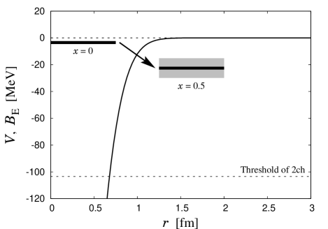
Figure 8: Interaction $V_{11}$ (82) as a function of the radial coordinate $r$ with its strength $v_{0}=-650\text{ MeV}$ and $v_{1}=0$. We also show the binding energies of the discrete bound states $B_{\rm E}\equiv m_{1}+M_{1}-\text{Re}\,E_{\rm pole}$ with $x=0$ and $x=0.5$. The shaded band for $x=0.5$ indicates the range of $B_{\rm E}\pm\text{Im}\,E_{\rm pole}$.

We first fix $v_{1}=0$ and $x=0$, and solve the Lippmann–Schwinger equation (38) by taking into account only the channel $1$. The interaction $V_{11}(r)$ is plotted as a function of the radial coordinate $r$ in Fig. 8. In this condition we have a $0s$ bound state at the eigenvalue $E_{\rm pole}=1431.1\text{ MeV}$ with the binding energy $B_{\rm E}\equiv m_{1}+M_{1}-E_{\rm pole}=3.5\text{ MeV}$. For this bound state, we have checked that we can extract the two-body wave function as the residue of the scattering amplitude at the pole of the bound state, with the compositeness exactly unity.

Table 1: Properties of the resonance state in the coupled-channels interaction (82). The parameters are fixed as $b=0.5\text{ fm}$, $v_{0}=-650\text{ MeV}$, $v_{1}=0$, $x=0.5$, and $\theta=20^{\circ}$. The binding energy $B_{\rm E}$ and width $\Gamma$ are defined as $B_{\rm E}\equiv m_{1}+M_{1}-\text{Re}\,E_{\rm pole}$ and $\Gamma\equiv-2\,\text{Im}\,E_{\rm pole}$, respectively.

$B_{\rm E}$ [MeV]	$22.6$
$\Gamma$ [MeV]	$14.7$
$X_{1}$	$0.99-0.08i$
$X_{2}$	$0.01+0.08i$
$X_{1}+X_{2}$	$1.00+0.00i$
$U$	$0.07$
$\tilde{X}_{1}$	$0.93$
$\tilde{X}_{2}$	$0.07$

Figure 9: Density distributions $\text{P}(q)$ obtained from the Schrödinger equation (Schr) and Lippmann–Schwinger equation (LS) with the interaction parameters $v_{0}=-650\text{ MeV}$, $v_{1}=0$ and $x=0.5$. The scaling angle is $\theta=20^{\circ}$.

Now let us switch on the coupling with nonzero $x$. We here take $x=0.5$, with which the $0s$ bound state in the channel $1$ becomes a resonance state. The eigenenergy $E_{\rm pole}$ is $1412.0-7.3\text{ MeV}$, which is also shown in Fig. 8. The properties of this resonance state is listed in Table 1. In Fig. 9, we show the density distributions from the Schrödinger equation (65) and Lippmann–Schwinger equation (68). We note that, while the wave function from the Schrödinger equation is normalized by hand so that the sum of the compositeness in two channels is exactly unity, that from the Lippmann–Schwinger equation is automatically scaled. Amazingly, the wave functions from two equations coincide with each other. In particular, since the wave function from the Schrödinger equation is normalized, we can see that the wave function from the Lippmann–Schwinger equation is also correctly normalized. This result indicates that even for a resonance state in a coupled-channels problem we can extract the wave function from the scattering amplitude at the pole position. In Table 1, we also list the value of the compositeness from the Lippmann–Schwinger equation. From the result, the compositeness in the channel $1$, $X_{1}$, dominates the normalization $X_{1}+X_{2}=1$, which implies that this resonance state is a bound state of two particles in the channel $1$ with a coupling to the decaying channel $2$. We have checked that the normalization $X_{1}+X_{2}=1$ is obtained for resonance wave functions from the scattering amplitude with any different value of the parameter $x$.

In order to interpret the complex compositeness of each channel $X_{1,2}$, we calculate $\tilde{X}_{1,2}$ together with $U$ in Eqs. (54) and (55). The values of these quantities for the present resonance state are listed in Table 1. Because the present state gives $U=0.07\ll 1$, according to the discussion given after Eq. (56) we can safely interpret $\tilde{X}_{1}$ ($\tilde{X}_{2}$) as the probability to find the two-body component of channel $1$ ($2$). From the numerical result, we can conclude that this resonance is indeed a bound state of two particles in channel $1$.

Figure 10: Compositeness $X$ as a function of $v_{1}$. Lines and points are obtained from the formulae in Eqs. (73) and (84), respectively, with the wave function from the scattering amplitude.

Next we change the value of $v_{1}$ so as to introduce the energy dependence of the interaction. We take $E_{0}=E_{\rm pole}$ so that the pole position does not change. The wave function is calculated from the scattering amplitude. The behavior of the compositeness in channel $1$ and the sum $X_{1}+X_{2}$ are shown in Fig. 10. As one can see, the real part of $X_{1}+X_{2}$ as well as that of $X_{1}$ decreases when $v_{1}$ takes negatively larger values, which implies that the contribution form missing states becomes important in this condition. This result is consistent with that in the previous subsections. In addition, we note that, while sum $X_{1}+X_{2}$ becomes unity for $v_{1}=0$, it becomes complex for $v_{1}\neq 0$.

The value of the compositeness is compared with that from the continuity equation in the energy-dependent interaction. Actually, for a resonance state in a coupled-channels problem, one can straightforwardly extend the formula (81), which result in

$$X_{\partial V/\partial E}=1+e^{-6i\theta}\sum_{j,k}\int_{0}^{\infty}dq\frac{q^{2}}{2\pi^{2}}R_{j}(qe^{-i\theta})$$

$$\times\int_{0}^{\infty}dq^{\prime}\frac{q^{\prime\,2}}{2\pi^{2}}R_{k}(q^{\prime}e^{-i\theta})\frac{\partial V_{L,jk}}{\partial E}(E_{\rm pole};\,qe^{-i\theta},\,q^{\prime}e^{-i\theta}).$$ (84)

The result of $X_{\partial V/\partial E}$ with the wave function from the scattering amplitude is shown in Fig. 10 as points. From the figure, the points exactly lies on the lines of $X_{1}+X_{2}$, which means that the sum $X_{1}+X_{2}$ correctly reproduces the effect of the energy-dependent interaction in (84).

In summary, even for an unstable resonance state in a coupled-channels case, we can extract its two-body wave function from the scattering amplitude as the residue of the scattering amplitude at the resonance pole. The wave function from the scattering amplitude is automatically scaled in calculating the Lippmann–Schwinger equation at the resonance pole. In particular, we find that the sum of the compositeness is exactly unity for the energy-independent interaction, but it deviates from unity for the energy-dependent interaction, which can be interpreted as the missing-channel contribution. This result indicates that our scheme is valid even for an unstable resonance state in a coupled-channels problem, which will be essential when we investigate the hadronic molecular components for hadronic resonances in a coupled-channels approach.

III.4 A “bound state” of an unstable constituent

Finally we consider a “bound state” which contains an unstable constituent. This bound state is intrinsically unstable due to the decay of the unstable constituent particle. An example is a bound state of the $\sigma$ meson and nucleon, if it existed, since the $\sigma$ meson decays into $\pi\pi$ in the $\sigma N$ bound state as well as in free space. We evaluate the scattering amplitude of the unstable particle $A$ and stable particle $B$ by introducing the self-energy for $A$ in a method developed in Ref. Kamano:2008gr . Then, we extract the two-body wave function of the $AB$ bound state from the scattering amplitude. In this subsection we take the semirelativistic formulation.

In order to calculate the two-body wave function of the $AB$ bound state, we first describe the unstable constituent $A$. In this study we consider a case that a bare particle of mass $m_{\rm bare}$ couples to a two-body decay channel in $s$ wave to be a physical $A$. We assume that the two particles in the decay channel have the same mass $m_{d}$, which should satisfy $2m_{d}<m_{\rm bare}$ so that $A$ decays.

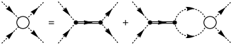
Figure 11: Diagram for the description of the physical unstable particle $A$. Double and dashed lines represent the bare particle and decay channel for $A$, respectively.

Suppose that the coupling of the bare particle for $A$ and the decay channel is controlled by

$$f(q)=\frac{\alpha\lambda^{2}}{q^{2}+\lambda^{2}}$$ (85)

with the magnitude of the relative momentum in the decay channel $q$, a coupling constant $\alpha$, and a cutoff $\lambda$. Because of this coupling, the bare particle becomes an unstable physical state $A$ in the two-body system of the decay channel. Actually, the physical state $A$ appears as the pole of the scattering amplitude for the decay channel, which can be described by the Lippmann–Schwinger equation (see Fig. 11):

$$\mathcal{T}(E_{2};\,q^{\prime},\,q)=\mathcal{V}(E_{2};\,q^{\prime},\,q)$$

$$+\int\frac{d^{3}k}{(2\pi)^{3}}\frac{\mathcal{V}(E_{2};\,q^{\prime},\,k)\mathcal{T}(E_{2};\,k,\,q)}{E_{2}-\mathcal{E}_{d}(k)},$$ (86)

with the total energy of the bare particle-decay channel system $E_{2}$, the energy of the on-shell particles in the decay channel $\mathcal{E}_{d}(q)\equiv 2\sqrt{q^{2}+m_{d}^{2}}$, and the “interaction” between two particles in the decay channel via the bare particle, $\mathcal{V}$:

$$\mathcal{V}(E_{2};\,q^{\prime},\,q)\equiv\frac{f(q^{\prime})f(q)}{E_{2}-m_{\rm bare}}.$$ (87)

After a simple algebra with ansatz $\mathcal{T}\propto f(q^{\prime})f(q)$, we can solve the Lippmann–Schwinger equation (86) and obtain the equation for the physical mass of the unstable particle $A$, $m_{\rm phys}$, from its bare mass $m_{\rm bare}$:

$$m_{\rm phys}=m_{\rm bare}+\int\frac{d^{3}k}{(2\pi)^{3}}\frac{f(k)^{2}}{m_{\rm phys}-\mathcal{E}_{d}(k)}.$$ (88)

We note that $m_{\rm phys}$ has an imaginary part when $2m_{d}<m_{\rm bare}$.

Let us fix the parameters $m_{\rm bare}=600\text{ MeV}$, $m_{d}=138.0\text{ MeV}$, $\alpha=0.15\text{ MeV}^{-1/2}$ and $\lambda=600\text{ MeV}$. In this condition we obtain the physical mass (88) as $m_{\rm phys}=422.7-52.0i\text{ MeV}$. Interestingly, we can calculate the compositeness of the decay channel for this physical unstable particle $A$ from the scattering amplitude (86) in our scheme, which results in $X_{d}=0.10+0.29i$. This indicates that we see only subdominant component of the decay channel inside $A$ since its absolute value, $|X_{d}|=0.31$, is negligible compared to unity.

Figure 12: Diagram for the self-energy of an unstable particle $A$ in the $AB$ propagator. Dashed lines represent the decay channel for $A$.

Now we consider the Schrödinger equation and Lippmann–Schwinger equation for the two-body system of this unstable particle $A$ and the stable particle $B$ of mass $M$. Since the unstable particle $A$ decays and its physical mass $m_{\rm phys}$ has an imaginary part, we should rewrite both the equations in an appropriate way. This can be done by introducing the self-energy for the unstable particle $\Sigma(E_{3};\,q)$, where $E_{3}$ is the eigenenergy of the whole system and $q$ is the magnitude of the relative momenta between $A$ and $B$ (see a diagram for the self-energy in Fig. 12). We employ the approach developed in Ref. Kamano:2008gr and formulate the self-energy as

$$\Sigma(E_{3};\,q)= \frac{m_{\rm bare}}{\sqrt{q^{2}+m_{\rm bare}^{2}}}\int\frac{d^{3}k}{(2\pi)^{3}}\frac{\mathcal{E}_{d}(k)}{\sqrt{\mathcal{E}_{d}(k)^{2}+q^{2}}}$$

$$\times\frac{f(k)^{2}}{E_{3}-\sqrt{q^{2}+M^{2}}-\sqrt{\mathcal{E}_{d}(k)^{2}+q^{2}}}.$$ (89)

By using this self-energy, we have to replace the two-body energy $\mathcal{E}(q)$ in the left-hand side of Schrödinger equation (23) with

$$\mathcal{E}_{\Sigma}(E_{3};\,q)=\sqrt{q^{2}+m_{\rm bare}^{2}}+\Sigma(E_{3};\,q)+\sqrt{q^{2}+M_{\phantom{j}}^{2}}.$$ (90)

In a similar manner, the two-body energy $\mathcal{E}(q)$ in the Lippmann–Schwinger equation (38) and in the compositeness formulation (52) should be replaced with the above $\mathcal{E}_{\Sigma}(E_{3};\,q)$. Then, momenta in every equation are transformed into the complex-scaled values in the complex scaling method so as to solve these equations for a resonance state.

For the interaction between $A$ and $B$, we employ the Yukawa function:

$$V(r)=\beta\frac{e^{-\mu r}}{r},$$ (91)

with the coupling constant $\beta$ and the interaction range $\mu$. The Fourier transformation of this interaction is

$$\tilde{V}(q)=\int d^{3}r\,V(r)e^{-i\bm{q}\cdot\bm{r}}=\frac{4\pi\beta}{q^{2}+\mu^{2}},$$ (92)

However, in the semirelativistic case the Yukawa interaction leads to an ultraviolet divergence for integrals. In order to tame the divergence, we introduce a form factor $\Lambda^{2}/(q^{2}+\Lambda^{2})$ with a cutoff $\Lambda$ as

$$\tilde{V}(q)=\frac{4\pi\beta}{q^{2}+\mu^{2}}\frac{\Lambda^{2}}{q^{2}+\Lambda^{2}}$$ (93)

Then, we consider a bound state of the unstable $A$ and stable $B$. We fix the parameters as $M=938.9\text{ MeV}$, $\beta=-2.0$, $\mu=450\text{ MeV}$, and $\Lambda=1.0\text{ GeV}$. The parameters for the unstable $A$ are the same: $m_{\rm bare}=600\text{ MeV}$, $m_{d}=138.0\text{ MeV}$, $\alpha=0.15\text{ MeV}^{-1/2}$ and $\lambda=600\text{ MeV}$. As a result, we obtain an $s$-wave bound state of the unstable $A$ and stable $B$ at its pole position $1363.8-32.2i\text{ MeV}$.

Figure 13: Density distribution $\text{P}(q)$ obtained from the Schrödinger equation (Schr) and Lippmann–Schwinger equation (LS) for the bound state of unstable and stable particles. The scaling angle is $\theta=20^{\circ}$.

We now solve the Schrödinger and Lippmann–Schwinger equations to obtain the two-body wave function of the $AB$ bound state. We show in Fig. 13 the density distribution $\text{P}(q)$ calculated from the wave function in two equations. The one in the Schrödinger equation is normalized to be unity by hand, while the one in the Lippmann–Schwinger equation is extracted from the residue of the scattering amplitude without scaling factor. We note that the density distribution as well as the wave function becomes complex since the bound state is intrinsically resonance due to the unstable constituent.

As one can see, the density distributions from two equations do not coincide with each other. Both the real and imaginary parts from the Lippmann–Schwinger equation are smaller than those from the Schrödinger equation. Actually, the compositeness from the scattering amplitude is evaluated as $X=0.90-0.21i$, which is unity for the wave function from the Schrödinger equation. This fact can be interpreted as the effect of missing-channel contributions, in this case the decay channel of the unstable constituent $A$. In the present condition, this missing-channel contribution is implemented as the energy dependence of the self-energy $\Sigma$ for the unstable $A$ rather than the interaction.

Here we note that the compositeness $X=0.90-0.21i$ is slightly different from the value which satisfies the sum rule with $X_{d}$, i.e., we have $X+X_{d}=1.00+0.08i\neq 1$. This is because, in the present formulation, if $A$ is inside the bound state, the field renormalization constant for $A$ may change from the value in free space, which is nothing but $1-X_{d}$. This is caused by the fact that the self-energy for the particle $A$ inside the bound state depends on the whole energy $E_{3}$ and the relative momentum between $A$ and $B$, $q$. Indeed, in free space the self-energy for $A$ is $\Sigma(m_{\rm phys}+M;\,q=0)$, but this becomes $\Sigma(E_{\rm pole};\,q)$ inside the bound state, which can change the field renormalization constant for $A$ inside the bound state. Actually, we find that, when we neglect $q$ dependence of the self-energy $\Sigma$ and fix parameters so that $E_{\rm pole}\approx m_{\rm phys}+M$, the sum rule $X+X_{d}=1$ returns to be satisfied.

In summary, from the scattering amplitude we can extract the resonance wave function for a bound state which contains an unstable constituent. We have observed that the compositeness deviates from unity due to the decay channel for the unstable constituent as a missing contribution, although the sum rule of the compositeness is broken slightly by the shift of the field renormalization constant for the unstable constituent from the value in free space. This discussion will help us investigate, e.g., the $\sigma N$ and $\rho N$ components inside the $N^{\ast}$ and $\Delta^{\ast}$ resonances in a forthcoming paper Sekihara:2016 .

IV Summary

In this study we have established a way to evaluate the two-body wave functions of bound states, both in the stable and decaying cases, from the residue of the scattering amplitude at the pole position. An important finding is that the two-body wave functions of the bound states are automatically scaled when evaluated from the scattering amplitude. In particular, while the compositeness, defined as the norm of the two-body wave function, is unity for energy-independent interactions, it deviates from unity for energy-dependent interactions, which can be interpreted as missing-channel contributions. We have checked that our scheme works correctly by considering bound states in a single-channel problem and resonances in three cases: single-channel, coupled-channels, and unstable constituent cases.

We emphasize that the compositeness $X_{j}$ is not observable and hence in general a model dependent quantity. However, we can uniquely determine it from the scattering amplitude once we fix the model space, form of the kinetic energy $\mathcal{E}_{j}(q)$, and interaction. We also note that, while the resonance wave function depends on the scaling angle $\theta$ in the complex scaling method, the compositeness, or in general quantities as the integral of the wave function squared, is independent of the scaling angle since the complex-scaled momentum $qe^{-i\theta}$ can be interpreted as the change of the contour for the momentum integral of the range $[0,\,\infty)$ to the rotated one with the angle $-\theta$.

An important application of the scheme developed here is to investigate the internal structure of candidates of hadronic molecules. Actually, we can discuss the hadronic molecular component of hadronic resonances in terms of the compositeness, by constructing hadron–hadron scattering amplitudes in an effective model and extracting the two-body wave function from the amplitudes. In a forthcoming paper Sekihara:2016 , we will apply our present scheme to the physical $N^{\ast}$ and $\Delta^{\ast}$ resonances in a precise $\pi N$ scattering amplitude, and discuss the meson–baryon components for these resonances by the compositeness from the scattering amplitude. Finally we emphasize that, in general, the present scheme can be applied to resonances in any other models, such as $N^{\ast}$ and $\Delta^{\ast}$ resonances in the dynamical approaches of ANL–Osaka Kamano:2013iva and Jülich Ronchen:2012eg , as long as they fully solve the Lippmann–Schwinger equation.

- (1) S. Weinberg, Phys. Rev. 137, B672 (1965).
- (2) V. Baru, J. Haidenbauer, C. Hanhart, Y. Kalashnikova and A. E. Kudryavtsev, Phys. Lett. B 586, 53 (2004).
- (3) T. Hyodo, Phys. Rev. Lett. 111, 132002 (2013).
- (4) T. Hyodo, Phys. Rev. C 90, 055208 (2014).
- (5) C. Hanhart, J. R. Pelaez and G. Rios, Phys. Lett. B 739, 375 (2014).
- (6) Y. Kamiya and T. Hyodo, Phys. Rev. C 93, 035203 (2016).
- (7) Y. Kamiya and T. Hyodo, PTEP 2017, in press [arXiv:1607.01899 [hep-ph]].
- (8) See, e.g., K. Gottfried and T. M. Yan, Quantum Mechanics: Fundamentals (Springer, New York, 2003), 2nd ed., Sec. 8.2 (c).
- (9) E. Hernandez and A. Mondragon, Phys. Rev. C 29, 722 (1984).
- (10) D. Gamermann, J. Nieves, E. Oset and E. Ruiz Arriola, Phys. Rev. D 81, 014029 (2010).
- (11) J. Yamagata-Sekihara, J. Nieves and E. Oset, Phys. Rev. D 83, 014003 (2011).
- (12) T. Hyodo, D. Jido and A. Hosaka, Phys. Rev. C 85, 015201 (2012).
- (13) T. Hyodo, Int. J. Mod. Phys. A 28, 1330045 (2013).
- (14) F. Aceti and E. Oset, Phys. Rev. D 86, 014012 (2012).
- (15) T. Sekihara and T. Hyodo, Phys. Rev. C 87, 045202 (2013).
- (16) C. W. Xiao, F. Aceti and M. Bayar, Eur. Phys. J. A 49, 22 (2013).
- (17) F. Aceti, L. R. Dai, L. S. Geng, E. Oset and Y. Zhang, Eur. Phys. J. A 50, 57 (2014).
- (18) F. Aceti, E. Oset and L. Roca, Phys. Rev. C 90, 025208 (2014).
- (19) H. Nagahiro and A. Hosaka, Phys. Rev. C 90, 065201 (2014).
- (20) T. Sekihara, T. Hyodo, and D. Jido, PTEP 2015, 063D04 (2015).
- (21) C. Garcia-Recio, C. Hidalgo-Duque, J. Nieves, L. L. Salcedo and L. Tolos, Phys. Rev. D 92, 034011 (2015).
- (22) T. Sekihara, T. Arai, J. Yamagata-Sekihara and S. Yasui, Phys. Rev. C 93, 035204 (2016).
- (23) Z. H. Guo and J. A. Oller, Phys. Rev. D 93, 054014 (2016).
- (24) Z. H. Guo and J. A. Oller, Phys. Rev. D 93, 096001 (2016).
- (25) S. Aoyama, T. Myo, K. Kato and K. Ikeda, Prog. Theor. Phys. 116, 1 (2006).
- (26) T. Sekihara, in preparation.
- (27) G. Gamow, Z. Phys. 51, 204 (1928).
- (28) N. Hokkyo, Prog. Theor. Phys. 33, 1116 (1965).
- (29) T. Berggren, Nucl. Phys. A 109, 265 (1968).
- (30) W. Romo, Nucl. Phys. A 116, 618 (1968).
- (31) R. Machleidt, Phys. Rev. C 63, 024001 (2001).
- (32) J. Formánek, R. J. Lombard, J. Mareš Czech. J. Phys. 54, 289 (2004).
- (33) K. Miyahara and T. Hyodo, Phys. Rev. C 93, 015201 (2016).
- (34) T. Sekihara, T. Hyodo and D. Jido, Phys. Rev. C 83, 055202 (2011).
- (35) H. Kamano, B. Julia-Diaz, T.-S. H. Lee, A. Matsuyama and T. Sato, Phys. Rev. C 79, 025206 (2009).
- (36) H. Kamano, S. X. Nakamura, T.-S. H. Lee and T. Sato, Phys. Rev. C 88, 035209 (2013).
- (37) D. Ronchen et al., Eur. Phys. J. A 49, 44 (2013).