Energy dynamics in a generalized compass chain

Abstract

We investigate the energy dynamics in a generalized compass chain under an external magnetic field. We show that the energy current operators act on three contiguous sites in the absence of the magnetic field, and they are incorporated with inhomogenous Dzyaloshinskii-Moriya interactions in the presence of the magnetic field. These complex interactions remain the Hamiltonian be an exactly solvable spin model. We study the effects of the three-site interactions and the Dzyaloshinskii-Moriya interactions on the energy spectra and phase diagram. The results have revealed that the energy current of the pristine quantum compass model is conserved due to the associated intermediate symmetries, and for other general cases such characteristic does not exist.

I Introduction

Һ The compass model has been coined as a minimal model to describe orbital-orbital interactions in strongly correlated electron systems three decades ago, and it regained people’s interest in much wider fields recently Nus15 . Part of the reason for this revival is that the communities connected this mathematical model with potential application in quantum computing. A milestone in this context was Kitaev’s honeycomb model Kit06 , which has the virtue of being exactly solvable. This quintessential model was proven to host gapped and gapless quantum spin liquids with emergent Majorana fermion excitations obeying non-Abelian statistics, topological order and topological entanglement. Further, quantum compass model on a two-dimensional (2D) square lattice was found to be dual to toric code model in transverse magnetic field Vid09 and to Xu-Moore model Xu04 . The common structure of the compass model and the Kitaev model is their building blocks are the bond-directional interactions. In parallel a family of layered iridates A₂IrO₃, where relativistic spin-orbit coupling plays an important role, have been suggested as promising candidates of solid-state systems for Kitaev’s model Jac09 ; Cha10 .

A variation of 2D quantum compass model is an extension to one dimension, in which antiferromagnetic exchange interactions alternate between even and odd bonds Brzezicki07 . It can be treated as a zigzag edge limit of Kitaev’s honeycomb model along one of the three crystalline directions Feng07 . A one-dimensional (1D) generalized compass model (GCM) was proposed to capture more insight along zigzag chains You1 ; You2 ; You3 . For instance, the model is anticipated to describe frustrated spin exchanges in perovskites transition metal (TM) oxides rendered by the Peierls-type spin-phonon coupling along distorted TM-oxygen-TM bonds Mochizuki11 . The GCM includes a tunable angle $\theta$ to control the distortion relative to the chain direction $\mathbf{e}_{x}$. The Ising model appears at angles of zero and this situation changes fundamentally when the TM-oxygen-TM bond is $180^{\circ}$. Such a model was recently introduced for a 1D zigzag chain in an $(a,b)$ plane You1 , and may be realized in either layered structures of transition metal oxides Xiao11 , or optical lattices Simon11 ; Sun12 , as well as Co zigzag chains Dupe15 .

The GCM is advantageous for the analytical solvability for arbitrary angles, rather than only extreme cases of some models can be handled. Hence, a kaleidoscope of equilibrium properties has been scrutinized. An exact analytical solution for various thermodynamic quantities, such as the Helmholtz free energy, the entropy, and the specific heat, can be straightforwardly retrieved You2 . Recently possible observations of Majorana zero modes in 1D topological superconductors have stimulated the interest to study the transport dynamics of spin chains Mourik12 ; Sun16 . The finite-temperature conductivity of a few 1D integrable quantum many-body systems, including the Heisenberg spin-1/2 chain, the Hubbard model, and the supersymmetric t-J model, was shown to be dissipationless. The integrity inherits from a macroscopic number of conserved quantities in these systems Zotos97 . The effects of either magnetization currents or energy currents in the 1D transverse Ising model Antal97 , 1D transverse XX model Antal98 , 1D XY model with three-spin interactions Men15 , 1D XXZ model Ste15 ; Biella16 were investigated. Also, the entanglement entropy was adopted to study nonequilibrium dynamics of integrable system by a quantum quench in the presence of an energy current Das11 . In this paper, we study nonequilibrium steady states of the GCM by imposing a current on the system and the properties of the ground state thus generated.

II The Hamiltonian and energy current

The 1D GCM considered below is given by

$$H_{\rm GCM} = \sum_{i=1}^{N^{\prime}}J_{o}\tilde{\sigma}_{2i-1}(\theta)\tilde{\sigma}_{2i}(\theta)+J_{e}\tilde{\sigma}_{2i}(-\theta)\tilde{\sigma}_{2i+1}(-\theta).$$

Here we assume the 1D chain has $N$ sites with periodic boundary conditions, and $i=1,2,\cdots,N^{\prime}$ ($N^{\prime}$ $\equiv$ $N$/2) specifies the index of two-site unit cells. $J_{o}$ and $J_{e}$ denote the coupling strengths on odd and even bonds, respectively. The operator with a tilde sign is defined as linear combinations of $\{\sigma_{l}^{x},\sigma_{l}^{y}\}$ pseudospin components (Pauli matrices),

$$\tilde{\sigma}_{l}(\theta) \equiv \cos(\theta/2)\,\sigma_{l}^{x}+\sin(\theta/2)\,\sigma_{l}^{y}.$$ (2)

In Eq.(LABEL:Hamiltonian1) an arbitrary angle $\pm\theta/2$ relative to $\sigma_{l}^{x}$ is introduced to characterize the preferential easy axes of Ising-like interactions on an odd/even bond. With increasing the angle $\theta$, the frustration increases gradually when the model Eq.(LABEL:Hamiltonian1) interpolates between the Ising model at $\theta=0$ to the quantum compass model (QCM) at $\theta=\pi/2$ Cincio10 .

The model Eq.(LABEL:Hamiltonian1) was solved rigorously and the ground state is ordered along the easy axis as long as $\theta\neq\pi/2$. The case of the compass limit of the GCM (also called the 1D Kitaev chain in some literatures), i.e., $\theta=\pi/2$, is rather special, where the model allows for $N/2$ mutually commuting Z₂ invariants $\sigma_{2i-1}^{y}\sigma_{2i}^{y}$ ($\sigma_{2i}^{x}\sigma_{2i+1}^{x}$). These so called intermediate symmetries conduce to a macroscopic degeneracy of $2^{N/2-1}$ in the structure of the spin Hilbert space away from the isotropic point, and the degeneracy of $2^{N/2}$ due to the closure at energy band edges when the spin interactions are isotropic, i.e., $J_{\rm e}=J_{\rm o}$ You2 . In the thermodynamic limit we recover the degeneracy of $2\times 2^{N/2}$ for isotropic spin interactionsBrzezicki07 . We will unearth these intermediate symmetries not only lead to above ground-state degeneracies, but also admit a dissipationless energy current.

For a 1D compass chain, spin magnetizations are not conserved due to the intrinsic frustration in the compass model, and the only conserved quantity is the energy. We can decompose Eq.(LABEL:Hamiltonian1) into:

$$H_{\rm GCM} = \sum_{l=1}^{N^{\prime}}h_{l},$$ (3)

where

$$h_{l}=J_{o}\tilde{\sigma}_{2l-1}(\theta)\tilde{\sigma}_{2l}(\theta)+J_{e}\tilde{\sigma}_{2l}(-\theta)\tilde{\sigma}_{2l+1}(-\theta).$$ (4)

A local energy operator $h_{l}$ contains interactions on two bonds. Further we can obtain the commutation relations:

$$[\tilde{\sigma}_{i}(\theta),\tilde{\sigma}_{j}(\theta)]=0,[\tilde{\sigma}_{i}(\theta),\tilde{\sigma}_{j}(-\theta)]=-2i\sin\theta\sigma_{i}^{z}\delta_{ij},$$

$$[\tilde{\sigma}_{i}(-\theta),\tilde{\sigma}_{j}(\theta)]=2i\sin\theta\sigma_{i}^{z}\delta_{ij},[\tilde{\sigma}_{i}(-\theta),\tilde{\sigma}_{j}(-\theta)]=0.$$

The energy current $\hat{J}_{l}$ of a compass chain in the nonequilibrium steady states is calculated by taking a time derivative of the energy density and follows from the continuity equationAntal97 :

$$\frac{dh_{l}}{dt}=i[{\cal H},h_{l}]=-\frac{\hat{j}_{2l+1}-\hat{j}_{2l-1}}{2}=-{\rm div}\hat{j}_{l}.$$ (5)

Immediately it arrives

$$\hat{j}_{2l-1}=-4J_{o}J_{e}\sin\theta\tilde{\sigma}_{2l-2}(-\theta)\sigma_{2l-1}^{z}\tilde{\sigma}_{2l}(\theta).$$ (6)

This energy current operator acts on three adjacent sites and has the $z$ component of spin-1/2 operators between two odd sites. Of course the odevity of operators is artificial. In order to maintain translational invariance of local energy densities, we set

$$h_{l}^{{}^{\prime}}=J_{e}\tilde{\sigma}_{2l}(-\theta)\tilde{\sigma}_{2l+1}(-\theta)+J_{o}\tilde{\sigma}_{2l+1}(\theta)\tilde{\sigma}_{2l+2}(\theta).$$ (7)

Then we can derive

$$\hat{j}_{2l}=4J_{o}J_{e}\sin\theta\tilde{\sigma}_{2l-1}(\theta)\sigma_{2l}^{z}\tilde{\sigma}_{2l+1}(-\theta).$$ (8)

Therefore, a linear combination gives rise to

$$\hat{J}_{l} = \frac{1}{2}(\hat{j}_{2l}+\hat{j}_{2l+1})$$ (9)

$$= 2J_{o}J_{e}\sin\theta\Big{[}\tilde{\sigma}_{2l-1}(\theta)\sigma_{2l}^{z}\tilde{\sigma}_{2l+1}(-\theta)$$

$$- \tilde{\sigma}_{2l}(-\theta)\sigma_{2l+1}^{z}\tilde{\sigma}_{2l+2}(\theta)\Big{]}.$$

The local energy operator in the Hamiltonian Eq.(LABEL:Hamiltonian1) involves two sites ($i$, $i$+1), while the local energy current operator embraces three sites ($i$-1, $i$, $i$+1). The form of energy current operator Eq.(9) is generally angle dependent. For $\theta$=0, the operator will present an XZX type although the front factor will vanish. While it exhibits an XZY$-$YZX type in the compass limit.

The macroscopic current $\hat{J}_{E}=\sum_{l}\hat{J}_{l}$ sums over all sites of the local currents. The presence of an effective energy flow will manifest itself in the effective Hamiltonian ${\cal H}$ followed by a Lagrange multiplier $\lambda$:

$${\cal H} = H_{\rm GCM}-\lambda\sum_{i}\hat{J}_{i},$$ (10)

In the following we set $J^{*}$ $\equiv$ $-2\lambda J_{o}J_{e}\sin\theta$ to make the formulas concise. Finding the ground state of ${\cal H}$ gives us the minimum energy state of $H_{\rm GCM}$ which carries an energy current $\hat{J}_{E}$, and thus provide us with the properties of the nonequilibrium steady states.The Hamiltonian of the 1D GCM with three-site interactions is given by

$${\cal H} = H_{\rm GCM}+H_{\rm 3-site}.$$ (11)

The GCM is driven out of equilibrium by a quantum quench in the presence of an energy current. The current term reads

$$H_{\rm 3-site} = J^{*}\sum_{i}\Big{[}\tilde{\sigma}_{2i-1}(\theta)\sigma_{2i}^{z}\tilde{\sigma}_{2i+1}(-\theta)$$ (12)

$$- \tilde{\sigma}_{2i}(-\theta)\sigma_{2i+1}^{z}\tilde{\sigma}_{2i+2}(\theta)\Big{]}.$$

To better understand the current-carrying term, one can define new annihilation and creation operators for Majorana fermions: $\gamma_{i,1}$=$e^{-i\theta/2}c_{i}^{\dagger}$+$e^{i\theta/2}c_{i}$,$\gamma_{i,2}$=$i(e^{i\theta/2}c_{i}^{\dagger}$-$e^{-i\theta/2}c_{i})$ Kitaev01 . In this respect, we can verify $\gamma_{i,n}^{\dagger}$= $\gamma_{i,n}$, $\gamma_{i,n}^{2}$=1 ($n$=1,2), but $\gamma_{i,1}$$\gamma_{i,2}$$\neq$$-\gamma_{i,2}$ $\gamma_{i,1}$, $H_{\rm 3-site}$= $J^{*}$$\sum_{i}-i\gamma_{2i-1,2}\gamma_{2i+1,1}+i\gamma_{2i,2}\gamma_{2i+2,1}$. Here the Majorana operators $\gamma_{i,2}$, $\gamma_{i+2,1}$ from different sites are paired together and especially the whole chain can be seen as two separate chains.

Both the bare GCM and the energy current can be expressed into a Majorana fermions representation using the Jordan-Wigner transformation. We employ the standard Jordan-Wigner transformation which maps explicitly between quasispin operators and spinless fermion operators through the following relations Bar70 :

$$\sigma_{j}^{z} = 1-2c_{j}^{\dagger}c_{j},\quad\sigma_{j}^{y}=i\sigma_{j}^{x}\sigma_{j}^{z},$$

$$\sigma_{j}^{x} = \prod_{i<j}\,(1-2c_{i}^{\dagger}c_{i})(c_{j}+c_{j}^{\dagger}),$$ (13)

where $c_{j}$ and $c_{j}^{\dagger}$ are annihilation and creation operators of spinless fermions at site $j$ which obey the standard anticommutation relations, $\{c_{i},c_{j}\}=0$ and $\{c_{i}^{\dagger},c_{j}\}=\delta_{ij}$. To diagonalize the Hamiltonian Eq. (11), a Fourier transformation for plural spin sites is followed:

$$c_{2j-1}=\frac{1}{\sqrt{N^{\prime}}}\sum_{k}e^{-ikj}a_{k},\text{ \ \ }c_{2j}=\frac{1}{\sqrt{N^{\prime}}}\sum_{k}e^{-ikj}b_{k}.$$ (14)

Then we write it in a symmetrized matrix form with respect to the $k\leftrightarrow-k$ transformation within the Bogoliubov-de Gennes (BdG) representation,

$${\cal H} = \sum_{k}\,\Gamma_{k}^{\dagger}\,\hat{M}_{k}\,\Gamma_{k},$$ (15)

where

$$\hat{M}_{k}=\frac{1}{2}\left(\begin{array}[]{cccc}B_{k+}&-iJ^{*}\sin k&A_{k}&P_{k}+Q_{k}\\ iJ^{*}\sin k&B_{k-}&P_{k}-Q_{k}&-A_{k}\\ A_{k}^{*}&P_{k}^{*}-Q_{k}^{*}&B_{k-}&iJ^{*}\sin k\\ P_{k}^{*}+Q_{k}^{*}&-A_{k}^{*}&-iJ^{*}\sin k&B_{k+}\end{array}\right),$$ (20)

(21)

and $\Gamma_{k}^{\dagger}=(a_{k}^{\dagger},a_{-k},b_{k}^{\dagger},b_{-k}{})$. Here the discrete momentums are given by

$$k=\frac{n\pi}{N^{\prime}},\quad n=-(N^{\prime}-1),-(N^{\prime}-3),\ldots,N^{\prime}-1,$$ (22)

and the compact notations in Eq.(21) read

$$A_{k} = J_{o}+J_{e}e^{ik},B_{ks}=sJ^{*}\cos(\theta-sk),$$

$$P_{k} = i\sin\theta(J_{e}e^{ik}+J_{o}),Q_{k}=-\cos\theta(J_{e}e^{ik}-J_{o}).$$

The diagonalization of the Hamiltonian matrix Eq.(21) yields the energy spectra $\varepsilon_{k,j}$, ($j$=1, $\cdots$, 4). We plot the energy spectra for a few typical parameters in Figs. 1 and 2. We note due to the lack of parity ($P$) and time reversal ($T$) symmetries in three-site interactions, the spectra are nonsymmetric with respect to $k=0$. However, the BdG Hamiltonian (15) has been enlarged in an artificially particle-hole space and it still respects the particle-hole symmetry (PHS) ${\cal C}$, i.e., ${\cal C}\hat{M}_{k}{\cal C}=-\hat{M}_{-k}$, with ${\cal C}^{2}=1$. The PHS implies $\varepsilon_{k,j}$, ($j$=1, $\cdots$, 4) actually are two copies of the original excitation spectrum. To be specific, $\varepsilon_{k,4}$=-$\varepsilon_{-k,1}$, $\varepsilon_{k,3}$=-$\varepsilon_{-k,2}$, as is evidenced in Figs. 1 and 2. The bands with positive energies correspond to the electron excitations while the negative ones are the corresponding hole excitations. When all quasiparticles above the Fermi surface are absent the ground-state energy for the particle-hole excitation spectrum may be expressed as:

$$E_{0}=-\frac{1}{2}\sum_{k}\sum_{j=1}^{4}|\varepsilon_{k,j}|.$$ (23)

Accordingly, the gap is determined by the absolute value of the difference between the second and third energy branches,

$$\Delta=\min_{k}|\varepsilon_{k,2}-\varepsilon_{-k,3}|.$$ (24)

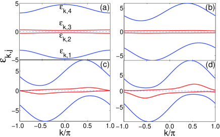
Figure 1: (Color online) The energy spectra $\varepsilon_{k,j}$ ($j=1,\cdots,4$) for increasing $J^{*}$: (a) $J^{*}$ = 0, (b) $J^{*}$ = 2, (c) $J^{*}$ = 4, and (d) $J^{*}$ = 6. Parameters are as follows: $J_{o}=1$, $J_{e}=4$, $\theta=\pi/3$.

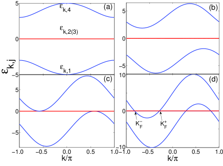
Figure 2: (Color online) The energy spectra $\varepsilon_{k,j}$ ($j=1,\cdots,4$) for increasing $J^{*}$: (a) $J^{*}$ = 0, (b) $J^{*}$ = 2, (c) $J^{*}$ = 4, and (d) $J^{*}$ = 6. $\varepsilon_{k,2}$ and $\varepsilon_{k,3}$ are degenerate at zero energies. Parameters are as follows: $J_{o}=1$, $J_{e}=4$, $\theta=\pi/2$.

III Three-site interactions

It is worth mentioning that three-spin interactions arise naturally in the Hubbard model as higher-order corrections and in the presence of a magnetic flux. Recently three-site interactions have received considerable attention from both theoretical side Got99 ; Tit03 ; Lou04 ; Kro08 ; Cheng10 ; Der11 ; Li11 ; Top12 ; Zhang15 ; Lei15 ; Ste15 ; Lah15 ; Brz14 and experimental side Tseng99 ; Peng09 ; Pachos04 . In the following we shall figure out effects of the emergent three-site interactions in the GCM.

Figure 3 show the gap $\Delta$ by adjusting the angle $\theta$ and the strength of three-site interactions $J^{*}$. We find $\theta_{c}=\pi/2$ and $J^{*}_{c}=2\sqrt{J_{o}J_{e}}$ are the critical lines. To understand various phases and the quantum phase transitions, we consider $\theta=\pi/3$ and $\theta=\pi/2$ separately, without losing generality. The eigenenergies for various $J^{*}$ are labeled sequentially from the bottom to the top as $\varepsilon_{k,1},\cdots,\varepsilon_{k,4}$ in Fig. 1 and Fig. 2. For $\theta=\pi/3$, the gap closes at $k=0$ at $J^{*}_{c}$ and reopens as $J^{*}$ increases. When $J^{*}$ is below $J^{*}_{c}$, a canted antiferromagnetic phase was identified. In the large $J^{*}$ limit, the spectra $\varepsilon_{k,3}$ and $\varepsilon_{k,4}$ will converge to $\epsilon_{+}(k)$ =$J^{*}(\sin\theta\sin k+\sqrt{\cos^{2}\theta+\sin^{2}\theta\sin^{2}k})$$>0$, while $\varepsilon_{k,1}$ and $\varepsilon_{k,2}$ will merge to $\epsilon_{-}(k)$ =$J^{*}(\sin\theta\sin k-\sqrt{\cos^{2}\theta+\sin^{2}\theta\sin^{2}k})$$<0$. A spiral phase is anticipated at large $J^{*}$ for $\theta$ $\neq$ $\pi/2$. Such criticality belongs to a second-order quantum phase transition. However, the quantum phase transition by varying $\theta$ is found to be within Berezinskii-Kosterlitz-Thouless scenario.

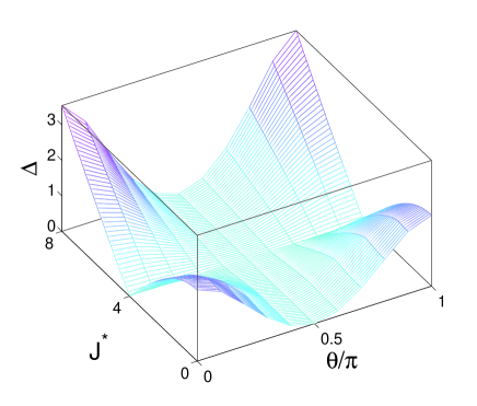
Figure 3: (Color online) The gap $\Delta$ as a function of $\theta$ and $J^{*}$. Parameters are as follows: $J_{o}$=1, $J_{e}$=4.

Note that

$$[\hat{J}_{E},H_{\rm GCM}]=4iJ_{o}J_{e}\sin\theta$$

$$\times \sum_{i}\Big{\{}J_{o}\Big{(}\tilde{\sigma}_{2i}(-\theta)\tilde{\sigma}_{2i+1}(\theta-\pi)-\tilde{\sigma}_{2i}(\theta-\pi)\tilde{\sigma}_{2i+1}(-\theta)\Big{)}$$

$$+ J_{e}\Big{(}\tilde{\sigma}_{2i-1}(-\theta-\pi)\tilde{\sigma}_{2i}(\theta)-\tilde{\sigma}_{2i-1}(\theta)\tilde{\sigma}_{2i}(-\theta-\pi)\Big{)}\Big{\}}.$$

We find that the global energy current operator $\hat{J}_{E}$ does not commute with the Hamiltonian for arbitrary $\theta$ except for the compass limit. In this special case ($\theta=\pi/2$), the energy current $\hat{J}_{E}$ is conserved, and thus the energy current time correlations should be independent of time. Such conclusion is a bit different from the finding in Ref.[Robin16, ], where the translation invariance of local energy densities is violated. The ground state of ${\cal H}$ can be considered as a current-carrying steady state of $H_{\rm GCM}$ at zero temperature, and the ground-state expectation value of current operator $J_{E}\equiv\langle\hat{J}_{E}\rangle$ acts as an order parameter indicating the presence of an energy current, as shown in Fig. 4. One can see the conservation of the current operator is crucial to the validity of being an order parameter.

Figure 4: (Color online) The energy current verse $J^{*}$ for $\theta=\pi/3$ and $\theta=\pi/2$. Parameters are as follows: $J_{o}=1$, $J_{e}=4$.

When $\theta=\pi/2$, the system is maximally frustrated. We can actually rotate the original $(\sigma^{x},\sigma^{y})$ plane clockwise by $\pi/4$ around $z$-axis, and then the transformed Hamiltonian in the new axis $(\bar{\sigma}^{x},\bar{\sigma}^{y})$ reads

$${\cal H} = \sum_{i=1}^{N^{\prime}}J_{o}\bar{\sigma}_{2i-1}^{x}\bar{\sigma}_{2i}^{x}+J_{e}\bar{\sigma}_{2i}^{y}\bar{\sigma}_{2i+1}^{y}$$ (26)

$$- J^{*}(\bar{\sigma}_{2i-1}^{x}\sigma_{2i}^{z}\bar{\sigma}_{2i+1}^{y}-\bar{\sigma}_{2i}^{y}\sigma_{2i+1}^{z}\bar{\sigma}_{2i+2}^{x}).$$

In this circumstance, the diagonlization of Hamiltonian matrix (21) yields the eigenspectra:

$$\varepsilon_{k,1}=J^{*}\sin k-|J_{o}+J_{e}e^{ik}|,\quad\varepsilon_{k,2(3)}=0,$$

$$\varepsilon_{k,4}=J^{*}\sin k+|J_{o}+J_{e}e^{ik}|.$$ (27)

One can easily find that three-site interactions commute with bare compass model. That is to say, the compass model and the three-site interactions have the same ground state for $J^{*}<J^{*}_{c}\equiv\max(J_{o},J_{e})$. As shown in Fig. 2, the compass model with three-site interactions (12) is gapless irrespective of the values of $J_{o}$, $J_{e}$ and $J^{*}$ for $\theta=\pi/2$. Nevertheless, the Fermi-surface topology and also the ground-state degeneracy undergo changes upon increase $J^{*}$. For $J^{*}<J^{*}_{c}$, $\varepsilon_{k,2}$ and $\varepsilon_{k,3}$ dwell on zero energies, and thus gives rise to a macroscopic degeneracy originating from the intermediate symmetriesBrzezicki07 ; You07 . We can sum over the eigeneneries below the Fermi surface and obtain the ground-state energy:

$$E_{0}=-\frac{|J_{e}-J_{o}|}{\pi}E\left[\frac{-4J_{o}J_{e}}{(J_{e}-J_{o})^{2}}\right],$$ (28)

where $E[\cdot]$ gives the complete elliptic integral. One discovers that $E_{0}$ is independent of $J^{*}$, implying three-site correlations are vanishing in this highly disordered spin-liquid phase, in which only short-range correlations $|\langle\tilde{\sigma}_{2i}^{y}\tilde{\sigma}_{2i+1}^{y}\rangle|$ and $|\langle\tilde{\sigma}_{2i-1}^{x}\tilde{\sigma}_{2i}^{x}\rangle|$ survive.

With the increase of $J^{*}$, the minimum of $\varepsilon_{k,4}$ bends down until it touches $\varepsilon=0$ at an incommensurate mode when $J^{*}$ reaches a threshold value; cf. Fig. 2(c). Further increase of $J^{*}$ leads to the bands inversion between $\varepsilon_{k,1}$ and $\varepsilon_{k,4}$. There is a negative-energy region of $\varepsilon_{k,4}$ in $k$ space shown in Fig. 2(d) between $k_{F}^{-}$ and $k_{F}^{+}$, depicted by $\cos k_{F}^{\pm}=-\mu\mp\sqrt{1+\mu^{2}-\nu}$ with $\mu=J_{o}J_{e}/{J^{*}}^{2}$ and $\nu=(J_{o}^{2}+J_{e}^{2})/{J^{*}}^{2}$. Therefore, beyond $J^{*}_{c}$, the Fermi sea starts to be populated by the modes in between the zeros of the single-particle spectrum $\varepsilon_{k,4}$ [i.e., between $k_{F}^{-}$, and $k_{F}^{+}$ in Fig. 2(d)], implying that the ground state is no longer that of $H_{\rm GCM}$. We plot the ground-state energy density $e_{0}=E_{0}/N$ and the generalized stiffness $\eta(J^{*})$=$-\partial^{2}e_{0}/\partial{J^{*}}^{2}$ versus $J^{*}$ in Fig.5. It is obvious the generalized stiffness is singular at $J^{*}_{c}$, suggesting a quantum phase transition induced by frustrated three-spin interactions.

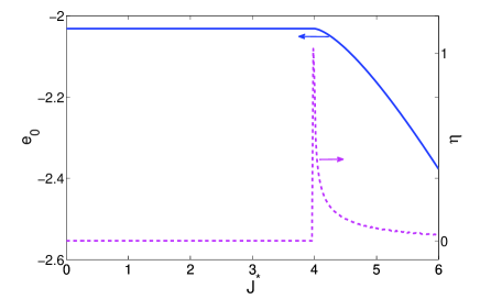
Figure 5: (Color online) The ground-state energy density $e_{0}$ and the generalized stiffness $\eta$ as a function of $J^{*}$. Parameters are as follows: $J_{o}$=1, $J_{e}$=4, $\theta=\pi/2$.

IV Effect of transverse field

We now consider the case where a magnetic field is oriented perpendicular to the easy plane of the spins, i.e., $\vec{h}$ = $h\hat{z}$. Here $h$ denotes the magnitude of the transverse external field. In this case, the Zeeman term is given by

$$H_{h}=h\hat{z}\cdot\sum_{i}^{N^{\prime}}(\vec{\sigma}_{2i-1}+\vec{\sigma}_{2i}).$$ (29)

Following a parallel procedure as above, we can derive the energy density using local energy operators

$$h_{l}^{{}^{\prime\prime}} = J_{o}\tilde{\sigma}_{2l-1}(\theta)\tilde{\sigma}_{2l}(\theta)+J_{e}\tilde{\sigma}_{2l}(-\theta)\tilde{\sigma}_{2l+1}(-\theta)$$ (30)

$$+ h(\sigma_{2l-1}^{z}+\sigma_{2l}^{z})$$

and commutation relation

$$[\tilde{\sigma}_{i}(\theta),\sigma_{j}^{z}]=2i\delta_{ij}\tilde{\sigma}_{i}(\theta-\pi).$$ (31)

One can find the transverse field will induce an extra term of energy current operator in comparison with the case when the magnetic field is absent:

$$\hat{J}_{l}^{h} = hJ_{o}\Big{[}\tilde{\sigma}_{2l-1}(\theta-\pi)\tilde{\sigma}_{2l}(\theta)-\tilde{\sigma}_{2l-1}(\theta)\tilde{\sigma}_{2l}(\theta-\pi)\Big{]}$$

$$+ hJ_{e}\Big{[}\tilde{\sigma}_{2l}(-\theta-\pi)\tilde{\sigma}_{2l+1}(-\theta)-\tilde{\sigma}_{2l}(-\theta)\tilde{\sigma}_{2l+1}(-\theta-\pi)\Big{]}.$$

We can easily observe that spin components in Eq.(LABEL:Jl23) are always perpendicular to each others on adjacent sites. Surprisedly, summing up all the local operators and the field-induced current term can be simplified into a $\theta$-independent form:

$$H_{\rm DM} = E\sum_{i}\Big{[}J_{o}({\sigma}_{2i-1}^{x}{\sigma}_{2i}^{y}-{\sigma}_{2i-1}^{y}\sigma_{2i}^{x})$$ (33)

$$+ J_{e}({\sigma}_{2i}^{x}{\sigma}_{2i+1}^{y}-{\sigma}_{2i}^{y}{\sigma}_{2i+1}^{x})\Big{]}.$$

In Eq.(33) we have set $E$ $\equiv$ $h\lambda^{{}^{\prime}}$ as an independent parameter describing the strength of field-induced current, where $\lambda^{{}^{\prime}}$ is the second Lagrange multiplier.

One can recognize $H_{\rm DM}$ describes well-known antisymmetric Dzyaloshinskii-Moriya exchange interactions Dzyaloshinskii , which have been incorporated to contribute to the ferroelectricity in the Katsura-Nagaosa-Balatsky (KNB) mechanism of the magnetoelectric effect Kat05 . To this end, the complete Hamiltonian with both two-site and three-site interactions takes the form:

$${\cal H}^{\prime} = H_{\rm GCM}+H_{\rm h}+H_{\rm DM}+H_{\rm 3-site}.$$ (34)

The ground state of ${\cal H}^{\prime}$ can be considered as a current-carrying steady state of $H_{\rm GCM}$ under external magnetic field at zero temperature. Subsequently, in Nambu representation, the Hamiltonian matrix $\hat{M}^{\prime}_{k}$ is modified in the following way,

$$\hat{M}_{k}\to\hat{M}^{\prime}_{k}=\hat{M}_{k}-h{\mathbb{I}}_{2}\otimes\sigma^{z}+\mathbb{R}_{k}e^{i\phi_{k}}\left(\begin{array}[]{cc }0&1\\ e^{-2i\phi_{k}}&0\\ \end{array}\right)\otimes\sigma^{x}.\\$$

Here ${\mathbb{I}}_{2}$ is a $(2\times 2)$ unity matrix, $\mathbb{R}_{k}=2E\sqrt{J_{o}^{2}+J_{e}^{2}-2J_{o}J_{e}\cos k}$ and $\phi_{k}=\tan^{-1}[(J_{o}-J_{e}\cos k)/J_{e}\sin k]$.

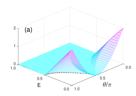
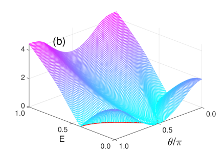
Figure 6: (Color online) The gap $\Delta$ as a function of $E$ and $\theta$ for (a) $J_{e}$=1 and (b) $J_{e}$=4. The dotted lines are given by Eq. (35). Parameters are as follows: $J_{o}$=1, $J^{*}=0$ and $h=0$.

The effect of an antisymmetric Dzyaloshinskii-Moriya interaction (DMI) and an external magnetic field has been studied in Ref.[You2, ]. The frustrated quantum spin can not simultaneously satisfy local energetic constraints of both interaction. The external magnetic field will spoil the Néel phase into the paramagnetic phase You1 . The homogeneous DMI will induce a gapless chiral phase with a nonlocal string order and a finite electrical polarization as long as $E>E_{c}\equiv\frac{1}{2}\sqrt{J_{o}J_{e}}\cos\theta$. As seen in Fig. 6(a), a gapless chiral phase arises accompanied by nonlocal string orders and finite electrical polarization for $E>E_{c}$ when $J_{o}$=$J_{e}$ You2 . Especially the chiral phase exists at infinitesimal $E$ for $\theta=\pi/2$. Interestingly enough, the effect of the inhomogeneous DMI [see Eq. (33)] plays a significantly different role from homogeneous one and it thus provides the system with a richer phase diagram. As is presented in Fig. 6(b), the induced phase has a dimerized gap when $E$ above the critical value

$$E_{c}\equiv\sqrt{J_{o}J_{e}}\cos\theta/(J_{o}+J_{e}).$$ (35)

The DMI leads to a spin-polarized current flowing through chiral magnetic structures and then may exert a spin-torque on the magnetic structure Bode07 . Specially in the compass limit, either a weak magnetic field or DMI can destroy the local order. In a similar way, the ground-state expectation of field-induced current operator $J^{h}_{E}\equiv\langle H_{\rm DM}\rangle/E$ is suitable for an order parameter exhibited in Fig.7 and it is independent of $h$.

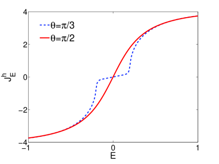
Figure 7: (Color online) The field-induced energy current verse $E$ for $\theta=\pi/3$ and $\theta=\pi/2$. Parameters are as follows: $J_{o}=1$, $J_{e}=4$.

V Summary and discussion

In this paper we have considered the energy transport in the one-dimensional generalized compass model, which interpolates between two qualitatively different well-known models in one dimension. It represents the Ising model for $\theta=0$ and the pristine quantum compass model for $\theta=\pi$/2. Although the system is highly frustrated, we have shown that exact solutions of the corresponding model may be obtained through Jordan-Wigner transformation. The longitudinal spin magnetization is not conserved due to the intrinsic frustration in the compass model, while the energy is nevertheless conserved, so the energy current operators $\hat{J}_{E}$ are well defined. We find the energy current operators $\hat{J}_{E}$ from the generalized compass model involve three contiguous sites, which can be diagonlized with the usual Jordan-Wigner and Bogoliubov transformations. Such multispin interactions break both the parity symmetry and the time-reversal symmetry and cause a reshuffling of the energy spectra. Our results show that the total energy current commutes with the Hamiltonian only in the compass limit, which means that the existence of conserved quantities is crucial for the presence of a persistent energy current. In this regard, the current operator can act as a natural order parameter in detecting the quantum phase transition from a non-current-carrying phase to a current-carrying phase.

We also investigated the general compass model in the presence of an external magnetic field. Consequently the current operators $\hat{J}_{E}$ will include additional Dzyaloshinskii-Moriya interactions. We find such homogeneous Dzyaloshinskii-Moriya interactions induce a chiral phase while inhomogeneous counterpart will conduce to a gapped phase.

To conclude, low dimensional quantum magnets with general exchange interactions cover a vast number of materials and theoretical models. The merit of the model considered here is its exact solvability that implies in particular the possibility to calculate accurately various static and dynamic quantities. The reported results may serve as a benchmark for more realistic cases which are not exactly solvable.

- (1) Z. Nussinov and J. van den Brink, Rev. Mod. Phys. 87, 1 (2015).
- (2) A. Kitaev, Annals of Physics 321, 2 (2006).
- (3) J. Vidal, R. Thomale, K. P. Schmidt, and S. Dusuel, Phys. Rev. B 80, 081104(R) (2009).
- (4) C. Xu and J. E. Moore, Phys. Rev. Lett. 93, 047003 (2004).
- (5) G. Jackeli and G. Khaliullin, Phys. Rev. Lett. 102, 017205 (2009).
- (6) J. Chaloupka, G. Jackeli, and G. Khaliullin, Phys. Rev. Lett. 105, 027204 (2010); 110, 097204 (2013); J. Chaloupka and G. Khaliullin, Phys. Rev. B 92, 043032 (2015).
- (7) W. Brzezicki, J. Dziarmaga, and A. M. Oleś, Phys. Rev. B 75, 134415 (2007).
- (8) X.-Y. Feng, G.-M. Zhang, and T. Xiang, Phys. Rev. Lett. 98, 087204 (2007).
- (9) W.-L. You, P. Horsch, and A. M. Oleś, Phys. Rev. B 89, 104425 (2014).
- (10) W.-L. You, G.-H. Liu, P. Horsch, and A. M. Oleś, Phys. Rev. B 90, 094413 (2014).
- (11) W.-L. You, Y.-C. Qiu, and A. M. Oleś, Phys. Rev. B 93, 214417 (2016).
- (12) Masahito Mochizuki, Nobuo Furukawa, and Naoto Nagaosa, Phys. Rev. Lett. 105, 037205 (2010); Phys. Rev. B 84, 144409 (2011).
- (13) D. Xiao, W. Zhu, Y. Ran, N. Nagaosa, and S. Okamoto, Nat. Commun. 2, 596 (2011).
- (14) J. Simon, W. S. Bakr, R. Ma, M. Eric Tai, P. M. Preiss, and M. Greiner, Nature (London) 472, 307 (2011).
- (15) G. Sun, G. Jackeli, L. Santos, and T. Vekua, Phys. Rev. B 86, 155159 (2012).
- (16) B. Dupé, J. E. Bickel, Y. Mokrousov, F. Otte, K. von Bergmann, A. Kubetzka, S. Heinze, and R. Wiesendanger, New J. Phys. 17, 023014 (2015).
- (17) V. Mourik, K. Zuo, S. M. Frolov, S. R. Plissard, E. P. A. M. Bakkers, L. P. Kouwenhoven, Science 336, 1003 (2012).
- (18) Hao-Hua Sun, Kai-Wen Zhang, Lun-Hui Hu, Chuang Li, Guan-Yong Wang, Hai-Yang Ma, Zhu-An Xu, Chun-Lei Gao, Dan-Dan Guan, Yao-Yi Li, Canhua Liu, Dong Qian, Yi Zhou, Liang Fu, Shao-Chun Li, Fu-Chun Zhang, and Jin-Feng Jia, Phys. Rev. Lett. 116, 257003 (2016).
- (19) X. Zotos and F. Naef, P. Prelovšek, Phys. Rev. B 55, 11029 (1997).
- (20) Tibor Antal, Zoltán Rácz and László Sasvári, Phys. Rev. Lett. 78, 167 (1997).
- (21) T. Antal, Z. Rácz, A. Rákos, and G. M. Schütz, Phys. Rev. E 57, 5184 (1998).
- (22) O. Menchyshyn, V. Ohanyan, T. Verkholyak, T. Krokhmalskii, and O. Derzhko, Phys. Rev. B 92, 184427 (2015).
- (23) Alberto Biella, Andrea De Luca, Jacopo Viti, Davide Rossini, Leonardo Mazza, and Rosario Fazio, Phys. Rev. B 93, 205121 (2016).
- (24) R. Steinigeweg, J. Gemmer, and W. Brenig, Phys. Rev. B 91, 104404 (2015).
- (25) Anirban Das, Silvano Garnerone, and Stephan Haas, Phys. Rev. A 84, 052317 (2011).
- (26) L. Cincio, J. Dziarmaga, and A. M. Oleś, Phys. Rev. B 82, 104416 (2010).
- (27) A. Kitaev, Physics-Uspekhi 44, 131 (2001).
- (28) E. Barouch and B. M. McCoy, Phys. Rev. A 2, 1075 (1970); 3, 786 (1971).
- (29) D. Gottlieb and J. Rössler, Phys. Rev. B 60, 9232 (1999).
- (30) I. Titvinidze and G. I. Japaridze, Eur. Phys. J. B 32, 383 (2003).
- (31) P. Lou, W.-C. Wu, and M.-C. Chang, Phys. Rev. B 70, 064405 (2004).
- (32) T. Krokhmalskii, O. Derzhko, J. Stolze, and T. Verkholyak, Phys. Rev. B 77, 174404 (2008).
- (33) V. Derzhko, O. Derzhko, and J. Richter, Phys. Rev. B 83, 174428 (2011).
- (34) M. Topilko, T. Krokhmalskii, O. Derzhko, and V. Ohanyan, Eur. Phys. J. B 85, 278 (2012).
- (35) W. W. Cheng and J.-M. Liu, Phys. Rev. A 81, 044304 (2010).
- (36) Yan-Chao Li and Hai-Qing Lin, Phys. Rev. A 83, 052323 (2011).
- (37) G. Zhang and Z. Song, Phys. Rev. Lett. 115, 177204 (2015).
- (38) S. Lei and P. Tong, Physica B 463, 1 (2015).
- (39) V. Lahtinen and E. Ardonne, Phys. Rev. Lett. 115, 237203 (2015).
- (40) W. Brzezicki and A. M. Oleś, Phys. Rev. B 90, 024433 (2014).
- (41) C. H. Tseng, S. Somaroo, Y. Sharf, E. Knill, R. Laflamme, T. F. Havel, and D. G. Cory, Phys. Rev. A 61, 012302 (1999).
- (42) X. Peng, J. Zhang, J. Du, and D. Suter, Phys. Rev. Lett. 103, 140501 (2009).
- (43) J. K. Pachos and M. B. Plenio, Phys. Rev. Lett. 93, 056402 (2004).
- (44) Robin Steinigeweg, and Wolfram Brenig, Phys. Rev. B 93, 214425 (2016).
- (45) W.-L. You, G.-S. Tian, and H.-Q. Lin, Phys. Rev. B 75, 195118 (2007).
- (46) I. Dzyaloshinskii, Phys. Chem. Solids 4, 241 (1958); T. Moriya, Phys. Rev. 120, 91 (1960).
- (47) H. Katsura, N. Nagaosa, and A. V. Balatsky, Phys. Rev. Lett. 95, 057205 (2005); M. Mostovoy, ibid. 96, 067601 (2006).
- (48) M. Bode, M. Heide, K. von Bergmann, P. Ferriani, S. Heinze, G. Bihlmayer, A. Kubetzka, O. Pietzsch, S. Blügel and R. Wiesendange, Nature 447, 190 (2007).