Implicit monotone difference methods for scalar conservation laws with source terms

Abstract

In this article, a concept of implicit methods for scalar conservation laws in one or more spatial dimensions allowing also for source terms of various types is presented. This material is a significant extension of previous work of the first author [3]. Implicit notions are developed that are centered around a monotonicity criterion. We demonstrate a connection between a numerical scheme and a discrete entropy inequality, which is based on a classical approach by Crandall and Majda. Additionally, three implicit methods are investigated using the developed notions. Next, we conduct a convergence proof which is not based on a classical compactness argument. Finally, the theoretical results are confirmed by various numerical tests.

1 Introduction

This article deals with the entropy solution of hyperbolic conservation laws in the sense of Kružkov. Specifically, we allow the numerical methods to act within the two most general settings, that is (i) smooth fluxes together with non-linear sources and (ii) continuous fluxes and sources depending both on space and time. The corresponding analytical existence and uniqueness results for these cases are given within a number of papers of Kružkov and his co-workers, see for example [1, 11, 12] and the references therein.

This paper represents a significant extension of the work by Breuß [3], where implicit methods are considered for homogeneous scalar equations in one dimension. To our knowledge, the combination of the developed concept of implicit methods for both mentioned general problems together with the application of corresponding schemes on problems belonging to both classes is new. Accordingly, the main contribution of this paper is the extension of the rigorously validated range of applicability of finite difference methods.

The encountered difficulties for the described task have already been discussed in the introduction of Breuß [3]. Summarizing, information that is propagated with infinite speed may take place provided that a flux function of a nonlinear conservation law is not Lipschitz continuous as it is accepted in setting (ii). A detailed one-dimensional example is given by Kružkov and Panov in [12] (see also [3]), where the exact solution is known. This example shows that a rarefaction wave extending to infinity after arbitrarily small time takes place. Additionally, this example has a pole for $u=0$ and the solution domain is infinite although an initial condition with compact support is given.

Two direct conclusions emerge from this example. At first, the Courant-Friedrichs-Lewy (CFL) number would be effectively zero provided an explicit scheme is used. Additionally, the Kuznetsov approach for convergence [13] is not employable, because it relies on a suitable error estimation which explicitly uses the Lipschitz continuity of the flux and the boundedness of the domain of the solution. At second, a variety of other well-established approaches for the convergence of numerical methods are not applicable. For instance, one approach is based on Helly’s theorem which uses the compactness of the function space of bounded variations (BV). This is employed in the convergence proofs of Total Variation Diminishing (TVD) methods. But using the BV concept, this function space is only compact (see LeVeque [14]) provided a fixed compact space-time-domain containing the solution is used. Hence, the compactness property of this function space is unfortunately not applicable in the discussed case. The same is true for explicit monotone methods as it is the case in the fundamental work of Crandall and Majda [5]. They used the properties of this function space to obtain a compactness argument. Especially, in that work the sources are also assumed to be essentially bounded and BV-stable integrable functions depending on space and time. In another important approach introduced by DiPerna [6] measure valued solutions are used, where the compactness of the domain of the solution both in space and time is assumed which has already been discussed in [4].

From this discussion it should be clear that we need to employ implicit schemes such that the convergence strategy is different from the before mentioned ones. Therefore, we use the monotonicity of implicit methods to obtain a discrete comparison principle. This suffices to guarantee the convergence of such methods to the entropy solution in the sense of Kružkov.

Therefore, in this paper the monotonicity property of an implicit scheme is investigated (see [7, 14] for the discussion for explicit schemes). Hence, it is indispensable to avoid any derivative of the flux. As we will show, we construct a monotonicity notion that is based on a comparison of data sets using an induction principle.

The application of this monotonicity notion on three implicit variations of well-known monotone explicit schemes is investigated. One would expect, that implicit schemes are generally capable to capture all effects described by a conservation law even for continuous fluxes and general sources, because in the implicit case the numerical characteristics include all the characteristics of the differential equation. However, while our monotonicity investigations of an implicit upwind scheme and an implicit Godunov-type method yield the expected results, the investigation of the implicit variation of the traditional Lax-Friedrichs scheme shows, that the scheme is only monotone even in the full implicit case if the flux is Lipschitz continuous. Furthermore, the restriction on the admissible Lipschitz constant of the flux is not depending on the number of spatial dimensions. This interesting result which is new to our knowledge is explored via a simple experiment using a two-dimensional linear advection equation.

This article consists of five additional sections. In Section 2, we briefly review the two most general theoretical results on solutions of conservation laws available to our knowledge, namely the existence and uniqueness results established in [1] and [10]. In the next section, we introduce the notions for implicit methods that are centered around monotonicity. The given detailed convergence proof is an extension of the strategy given in Breuß [3]. Section 4 presents the investigation of three numerical methods with respect to their monotonicity. Additionally, for these methods the proofs of convergence towards the entropy solution are given. Finally, we present the results of various numerical tests in Section 5 followed by a short summary and conclusive remarks in Section 6.

2 The setting

Within this section, we define the two mathematical scenarios of interest, i.e. we briefly review the type of problems considered in [1] and [10].

Scenario 1

The Cauchy problem under consideration is

$$\frac{\partial}{\partial t}u\left(\mathbf{x},t\right)+\sum_{l=1}^{d}\frac{\partial}{\partial x_{l}}f_{l}\left(u\left(\mathbf{x},t\right)\right)\,=\,q \mathbb{R}^{d}\times\left(0,T\right)\,,$$ on (1)

$$u\left(\mathbf{x},0\right)\,=\,u_{0}\left(\mathbf{x}\right) \mathbb{R}^{d}\,,$$ on (2)

where $T$ is a fixed positive number. Concerning the flux functions we generally assume

$$f_{l}(u)\in C\left(\mathbb{R};\,\mathbb{R}\right)\,,\quad l=1,\,\ldots,\,d\,.$$ (3)

In order to apply the uniqueness theorem given in [1], the fluxes are additionally supposed to satisfy the growth conditions

$$\left|f_{l}(u)-f_{l}(\hat{u})\right|\leq\omega_{l}(u-\hat{u})\;\textrm{ a.e. for }\;u\geq\hat{u}\;\textrm{ and for }\;l=1,\ldots,d\,,$$

with the moduli of continuity $\omega_{l}$ featuring

$$\omega_{1}(0)=\ldots=\omega_{d}(0)=0\quad\textrm{and}\quad\liminf_{r\to 0}r^{1-d}\prod_{l=1}^{d}\omega_{l}(r)<\infty\,.$$

Note that these conditions on the fluxes are more general than the usually assumed Lipschitz continuity. The initial condition shall satisfy

$$u_{0}\in L^{\infty}_{loc}\left(\mathbb{R}^{d};\,\mathbb{R}\right)\,,$$ (4)

and for the source term we consider

$$q\equiv q\left(\mathbf{x},t\right)\in L^{1}_{loc}\left(\mathbb{R}^{d}\times(0,T);\,\mathbb{R}\right)\,,$$ (5)

$$q(\cdot,t)\in L^{\infty}\left(\mathbb{R}^{d};\,\mathbb{R}\right)\;\textrm{ for a.e. }\;t\in(0,T)\;\textrm{ and }\;\int_{0}^{T}\|q(\cdot,t)\|_{\infty}\,\mathrm{d}t<\infty\,.$$ (6)

Under the conditions (3) – (6), Bénilan and Kružkov [1] proved uniqueness of the entropy solution of (1) – (2).

Because the solution of the Cauchy problem generally develops discontinuities even if $u_{0}$ is smooth, it is often considered in its weak form, i.e.

$$\int_{0}^{\infty}\int_{\mathbb{R}^{d}}\left[u\left(\mathbf{x},t\right)\phi_{t}\left(\mathbf{x},t\right)+\sum_{l=1}^{d}f_{l}(u\left(\mathbf{x},t\right))\frac{\partial}{\partial x_{l}}\phi\left(\mathbf{x},t\right)\right]\,\mathrm{d}\mathbf{x}\,\mathrm{d}t$$

$$= -\int_{\mathbb{R}^{d}}u_{0}\left(\mathbf{x}\right)\phi_{0}\left(\mathbf{x}\right)\,\mathrm{d}\mathbf{x}-\int_{0}^{\infty}\int_{\mathbb{R}^{d}}q\left(\mathbf{x},t\right)\phi\left(\mathbf{x},t\right)\,\mathrm{d}\mathbf{x}\,\mathrm{d}t\;\;\;\forall\phi\in C_{0}^{\infty}\left(\mathbb{R}^{d+1};\,\mathbb{R}\right)\,.$$ (7)

It is well-known that weak solutions are in general not unique, see for example [14] and the references therein. In order to ensure uniqueness, a so-called entropy condition has to be introduced. The already mentioned entropy condition due to Kružkov [1] which guarantees the uniqueness of a solution of (1) – (2) takes the form

$$\int_{0}^{\infty}\int_{\mathbb{R}^{d}}\Biggl{[}\mathopen{|}u\left(\mathbf{x},t\right)-k\mathclose{|}\phi_{t}\left(\mathbf{x},t\right)\Biggr{.}$$

$$\quad\quad\Biggl{.}+\sum_{l=1}^{d}\mathrm{sgn}\left(u\left(\mathbf{x},t\right)-k\right)\left[f_{l}(u\left(\mathbf{x},t\right))-f_{l}(k)\right]\frac{\partial}{\partial x_{l}}\phi\left(\mathbf{x},t\right)\Biggr{]}\,\mathrm{d}\mathbf{x}\,\mathrm{d}t$$

$$\geq -\int_{\mathbb{R}^{d}}\mathopen{|}u_{0}\left(\mathbf{x}\right)-k\mathclose{|}\phi_{0}\left(\mathbf{x}\right)\,\mathrm{d}\mathbf{x}$$

$$\quad-\int_{0}^{\infty}\int_{\mathbb{R}^{d}}\mathrm{sgn}\left[u\left(\mathbf{x},t\right)-k\right]q\left(\mathbf{x},t\right)\phi\left(\mathbf{x},t\right)\,\mathrm{d}\mathbf{x}\,\mathrm{d}t$$

$$\textrm{for all }\phi\in C_{0}^{\infty}\left(\mathbb{R}^{d+1};\,\mathbb{R}\right)\textrm{ with }\phi\geq 0\textrm{ and for all }k\in\mathbb{R}\,.$$

Scenario 2

The Scenario 2 deals with the Cauchy problem

$$\frac{\partial}{\partial t}u\left(\mathbf{x},t\right)+\sum_{l=1}^{d}\frac{d}{dx_{l}}f_{l}\left(\mathbf{x},t,u\left(\mathbf{x},t\right)\right)\,=\,q \mathbb{R}^{d}\times\left(0,T\right)\,,$$ on (9)

$$u\left(\mathbf{x},0\right)\,=\,u_{0}\left(\mathbf{x}\right) \mathbb{R}^{d}\,,$$ on (10)

where $T$ is a fixed positive number and with

$$\frac{d}{dx_{l}}f_{l}\equiv f_{l_{x_{l}}}+f_{l_{u}}u_{x_{l}}\,.$$

In comparison to Scenario 1, we impose different assumptions on the fluxes and the source terms. As in (4), there is no particular condition imposed on the initial data. The flux functions are now assumed to satisfy

$$f_{l}(\mathbf{x},t,u)\in C^{1}\left(\mathbb{R}^{d}\times\mathbb{R}_{+}\times\mathbb{R};\,\mathbb{R}\right)\,,\quad l=1,\,\ldots,\,d\,.$$ (11)

As source terms we consider functions

$$q\equiv q\left(\mathbf{x},t,u(\mathbf{x},t)\right)\in C^{1}\left(\mathbb{R}^{d}\times\mathbb{R}_{+}\times\mathbb{R};\,\mathbb{R}\right)\,.$$ (12)

Under the conditions (11) and (12), Kružkov [10] proved the uniqueness of the entropy solution of (9) – (10). Comparing the weak formulation of this problem with the weak formulation (7), we have to substitute

$$\int_{0}^{\infty}\int_{\mathbb{R}^{d}}q\left(\mathbf{x},t,u(\mathbf{x},t)\right)\phi\left(\mathbf{x},t\right)\,\mathrm{d}\mathbf{x}\,\mathrm{d}t\quad\textrm{for}\quad\int_{0}^{\infty}\int_{\mathbb{R}^{d}}q\left(\mathbf{x},t\right)\phi\left(\mathbf{x},t\right)\,\mathrm{d}\mathbf{x}\,\mathrm{d}t\,.$$ (13)

The assumptions (11) and (12) yield the form of the Kružkov entropy condition as

$$\int_{0}^{\infty}\int_{\mathbb{R}^{d}}\Biggl{[}\mathopen{|}u\left(\mathbf{x},t\right)-k\mathclose{|}\phi_{t}\left(\mathbf{x},t\right)\Biggr{.}$$

$$\quad\Biggl{.}+\sum_{l=1}^{d}\mathrm{sgn}\left(u\left(\mathbf{x},t\right)-k\right)\left[f_{l}(\mathbf{x},t,u\left(\mathbf{x},t\right))-f_{l}(\mathbf{x},t,k)\right]\frac{\partial}{\partial x_{l}}\phi\left(\mathbf{x},t\right)\Biggr{]}\,\mathrm{d}\mathbf{x}\,\mathrm{d}t$$

$$\quad\quad\geq -\int_{\mathbb{R}^{d}}\mathopen{|}u_{0}\left(\mathbf{x}\right)-k\mathclose{|}\phi_{0}\left(\mathbf{x}\right)\,\mathrm{d}\mathbf{x}$$

$$\quad-\int_{0}^{\infty}\int_{\mathbb{R}^{d}}\sum_{l=1}^{d}\mathrm{sgn}\left[u\left(\mathbf{x},t\right)-k\right]\left[q\left(\mathbf{x},t,u(\mathbf{x},t)\right)-f_{l_{x_{l}}}\left(\mathbf{x},t,k\right)\right]\phi\left(\mathbf{x},t\right)\,\mathrm{d}\mathbf{x}\,\mathrm{d}t$$

$$\textrm{for all }\phi\in C_{0}^{\infty}\left(\mathbb{R}^{d+1};\,\mathbb{R}\right)\textrm{ with }\phi\geq 0\textrm{ and for all }k\in\mathbb{R}\,.$$

3 Numerical methods

We first describe the implicit notions, followed by the proofs of the involved Lemmas and Theorems in a separate section. For the sake of brevity, we discuss only Scenario 1 in detail, since the techniques which have to be used with respect to Scenario 2 are identical. The proper conceptual extension to Scenario 2 is described within additional remarks.

3.1 A concept of implicit methods

Since we want to describe numerical methods in $d$ spatial dimensions, we spend some effort on a general notation.

Because we investigate finite difference methods, we have to introduce grid points. For simplicity, we consider grids which are equidistant with respect to the individual $d$ spatial dimensions as well as to time, i.e. we employ grid spacings $\Delta x_{l}$ corresponding to the space dimensions $l=1,\ldots,d$, and $\Delta t$ corresponding to time.

Since this results in a countable number of grid points, we introduce a linear numbering $J$ of the spatial grid points

$$J=\left\{0,1,2,\ldots\right\}\,.$$

We also define a bijective mapping

$$\tilde{J}\quad:\quad J \longrightarrow \mathbb{R}^{d}$$

$$i \longrightarrow \left(i_{1}\Delta x_{1},\,i_{2}\Delta x_{2},\,\ldots,\,i_{d}\Delta x_{d}\right)^{\mathrm{T}}\quad\textrm{with}\quad\left(i_{1},\,i_{2},\,\ldots,\,i_{d}\right)^{\mathrm{T}}\in\mathbb{Z}^{d}\,.$$

In order to describe the indices within the stencil of a numerical method, we define the index $i\pm\delta l$ via

$$i\pm\delta l\;\stackrel{{\scriptstyle\displaystyle{\tilde{J}}}}{{\longrightarrow}}\;\left(i_{1}\Delta x_{1},\,i_{2}\Delta x_{2},\,\ldots,\,\left(i_{l}\pm 1\right)\Delta x_{l},\,\ldots,\,i_{d}\Delta x_{d}\right)^{\mathrm{T}}\,.$$

Let $u_{j}^{k}$ and $q_{j}^{k}$ denote the value of the numerical solution and the value of the source term at the point with the index $j\in J$ at the time level $k\Delta t$, respectively. With these notations, we consider conservative implicit methods in the form

$$u_{j}^{n+1}=u_{j}^{n}-\sum_{l=1}^{d}\frac{\Delta t}{\Delta x_{l}}\left\{g_{l}\left(u_{j}^{n+1},\,u_{j+\delta l}^{n+1}\right)-g_{l}\left(u_{j-\delta l}^{n+1},\,u_{j}^{n+1}\right)\right\}+\Delta tq_{j}^{n+1}\,.$$ (15)

We assume that the numerical flux functions $g_{l}$ introduced in (15) are consistent, i.e.

$$g_{l}(v,\,v)=f_{l}(v)\textrm{ holds for all }v\in\mathbb{R}\textrm{ and for all }l=1,\,\ldots,\,d\,.$$

In the case of Scenario 2, we simply add arguments $(\mathbf{x}_{j},t^{n+1})$ within the fluxes; we will not do this explicitly in the following.

The key to nonlinear stability is the notion of monotonicity.

Definition 3.1 (Monotonicity).

Let two data sequences

$$v^{n}=\left\{v_{j}^{n}\right\}_{j\in J}\quad\textrm{and}\quad w^{n}=\left\{w_{j}^{n}\right\}_{j\in J}$$

be given. Let the investigated consistent and conservative numerical method produce new sequences of data $v^{n+1}$ and $w^{n+1}$ from the given data $v^{n}$ and $w^{n}$, respectively. Then the numerical method is monotone iff the implication

$$v^{n}\geq w^{n}\quad\Rightarrow\quad v^{n+1}\geq w^{n+1}$$ (16)

holds in the sense of the comparison of components.

It is useful to define $H$ and $\tilde{H}_{l}$ using $\underline{d}=\left\{1,\,\ldots,\,d\right\}$ via

$$u_{j}^{n+1} = H\left(l\in\underline{d},\,u_{j-\delta l}^{n+1},\,u_{j}^{n+1},\,u_{j+\delta l}^{n+1},\,u_{j}^{n}\right)$$ (17)

$$= u_{j}^{n}-\sum_{l=1}^{d}\frac{\Delta t}{\Delta x_{l}}\left\{g_{l}\left(u_{j}^{n+1},\,u_{j+\delta l}^{n+1}\right)-g_{l}\left(u_{j-\delta l}^{n+1},\,u_{j}^{n+1}\right)\right\}+\Delta tq_{j}^{n+1}$$

$$= u_{j}^{n}+\sum_{l=1}^{d}\tilde{H}_{l}\left(u_{j-\delta l}^{n+1},\,u_{j}^{n+1},\,u_{j+\delta l}^{n+1}\right)+\Delta tq_{j}^{n+1}\,.$$

Theorem 3.1 (Monotonicity of implicit methods).

Let $a$, $b$ and $c$ be arbitrarily chosen but fixed real numbers. A consistent and conservative implicit method of type (15) is monotone iff for all spatial dimensions $l\in\left\{1,\,\ldots,\,d\right\}$ holds

$$\tilde{H}_{l}\left(a+\Delta a,b,c\right)\quad\geq\quad\tilde{H}_{l}\left(a,b,c\right)\quad\forall\,\Delta a\geq 0\,,$$ (18)

$$\tilde{H}_{l}\left(a,b,c+\Delta c\right)\quad\geq\quad\tilde{H}_{l}\left(a,b,c\right)\quad\forall\,\Delta c\geq 0\,.$$ (19)

Note that we have omitted the condition

$$H\left(l\in\underline{d},\,u_{j-\delta l}^{n+1},\,u_{j}^{n+1},\,u_{j+\delta l}^{n+1},\,s+\Delta s\right)\geq H\left(l\in\underline{d},\,u_{j-\delta l}^{n+1},\,u_{j}^{n+1},\,u_{j+\delta l}^{n+1},\,s\right)$$

for all $j\in J$ and all $\Delta s\geq 0$, since this condition is redundant. This is due to the form of the method (15). Additionally, note that the monotonicity property does not depend on the exact nature of the source terms, i.e. both Scenario 1 and Scenario 2 are included within the range of applicability of Theorem 3.1.

Theorem 3.2 ($L_{\infty}$-Stability).

Let an implicit method of the form (15) be given, which is also conservative and monotone. Then the numerical solution is $L_{\infty}$-stable over any finite time interval $[0,T]$.

The following Definition is useful for proving convergence towards the entropy solution.

Definition 3.2 (Consistency with the entropy condition).

An implicit numerical scheme of type (15) is consistent with the entropy condition of Kružkov, if there exist for all $l=1,\,\ldots,\,d$ numerical entropy fluxes $G_{l}$ which satisfy for all $k\in\mathbb{R}$ the following assertions:

1. Consistency with the entropy flux of Kružkov

   $$G_{l}(v,v;k)=F_{l}(v;k)\textrm{ }\forall v\;\textrm{with}\;F_{l}(v;k)=\mathrm{sgn}(v-k)\left[f_{l}(v)-f_{l}(k)\right]\,.$$ (20)

2. Validity of a discrete entropy inequality

   $$\frac{U\left(u_{j}^{n+1};k\right)-U\left(u_{j}^{n};k\right)}{\Delta t}$$ (21)

   $$\leq -\sum_{l=1}^{d}\frac{G_{l}\left(u_{j}^{n+1},u_{j+\delta l}^{n+1};k\right)-G_{l}\left(u_{j-\delta l}^{n+1},u_{j}^{n+1};k\right)}{\Delta x_{l}}$$

   $$+\mathrm{sgn}\left[u_{j}^{n+1}-k\right]q_{j}^{n+1}\,,$$

   where $U(v;k)=\left|v-k\right|$ is chosen due to Kružkov.
   

In the sequel, we define

$$a\vee b:=\max(a,b)\quad\textrm{and}\quad a\wedge b:=\min(a,b)\,.$$ (22)

The important connection between the numerical entropy fluxes $G_{l}$ and the numerical flux functions $g_{l}$ is now established which are based on a variation of a procedure employed by Crandall and Majda [5].

Lemma 3.1.

Let a consistent and conservative numerical scheme of type (15) be given with numerical flux functions $g_{l}$, $l=1,\,\ldots,\,d$. Then the numerical entropy fluxes defined by

$$G_{l}(v,w;k)\;:=\;g_{l}(v\vee k,w\vee k)-g_{l}(v\wedge k,w\wedge k)$$ (23)

are consistent with the entropy fluxes of Kružkov.

One can now prove the following result, partly by a variation of the procedure given in [5]. We introduce the source term within the proof.

Theorem 3.3.

Let an implicit scheme of the form (15) be given, which is also consistent, conservative, and monotone. Then the scheme is also consistent with the entropy condition of Kružkov.

Under the same assumptions, we prove convergence of the corresponding numerical approximation to the entropy solution. We want to do this later when we concretely investigate numerical schemes.

3.2 Proofs

We first want to prove Theorem 3.1. The idea of the proof can be sketched as follows. Let two sequences $w^{n}$ and $w^{n+1}$ be given, where $w^{n+1}$ results from an application of a considered method on $w^{n}$. Then, a positive change in a given value $w_{j}^{n}$ inspires a positive change in $w_{j}^{n+1}$. Secondly, a positive change in $w_{j}^{n+1}$ inspires positive changes in $w_{j\pm\delta l}^{n+1}$ for all $l$, thus creating no oscillations. Thirdly, concerning an arbitrary index $i$, positive changes in $w_{i\pm\delta l}^{n+1}$ result in positive changes in $w_{i}^{n+1}$. Since the index $j$ used in the second argument is chosen arbitrarily, this is the same argument as the third one for $j\in\left\{i\pm\delta l;\,l=1,\,\ldots,\,d\right\}$. If and only if these conditions are fulfilled by a considered method, the method is monotone.

In order to give the proof of Theorem 3.1 a convenient structure, we first give the following Lemma.

Lemma 3.2.

Let a consistent and conservative implicit method of the form (15) be given, which satisfies the conditions (18) and (19). Furthermore, let two sequences $v^{n}=\left\{v_{j}^{n}\right\}_{j\in J}$ and $w^{n}=\left\{w_{j}^{n}\right\}_{j\in J}$ be given. Then from

$$\exists\,i\in J:\;v^{n}_{i}>w^{n}_{i}\quad\textrm{and}\quad\forall\,j\in\mathbf{J}\>(j\neq i):\;v^{n}_{j}=w^{n}_{j}$$

follows $v^{n+1}\geq w^{n+1}$ in the sense of the comparison of components.

Proof.

(of Lemma 3.2)
By the assumption of the Lemma there exists an index $i\in J$ so that $v_{i}^{n}>w_{i}^{n}$ holds. Without restriction of generality we choose $i=0$. The proof of the assertion follows by induction over suitable subsets of $J$.
Let us introduce these subsets. Therefore, let $J_{m}$ denote a subset of $J$ containing $m$ elements with

$$\forall\,m_{0}\in J_{m}\,\exists\,m_{1}\in J_{m}\,(m_{0}\neq m_{1}):\;\Bigl{[}\left\{m_{0}\right\}\cap\left\{p\in J_{m}\;;\;p=m_{1}\pm\delta l\textrm{, }l=1,\,\ldots,\,d\right\}\Bigr{]}\neq\emptyset$$

for $m\geq 2$, thus the elements of $J_{m}$ are indices of neighboring points.
Beginning of the induction: $m=1$
As indicated, we choose without restriction of generality $J_{1}=\left\{0\right\}$. The statement is true because of the form of the method (15), so that

$$H\left(l\in\underline{d},\,w_{-\delta l}^{n+1},\,w_{0}^{n+1},\,w_{\delta l}^{n+1},\,s+\Delta s\right)$$

$$\geq H\left(l\in\underline{d},\,w_{-\delta l}^{n+1},\,w_{0}^{n+1},\,w_{\delta l}^{n+1},\,s\right)\quad\forall\,\Delta s\geq 0\quad\textrm{holds.}$$

Assumption:
The statement is true for arbitrary but fixed $m>1$.
Induction step: $m\mapsto m+1$
Let the statement be true for the subsets $\left\{v_{i}^{n+1}\right\}_{i\in J_{m}}$ and $\left\{w_{i}^{n+1}\right\}_{i\in J_{m}}$ of the sequences $v^{n+1}$ and $w^{n+1}$. In particular, it holds

$$v_{\tilde{m}}^{n+1}\geq w_{\tilde{m}}^{n+1}\quad\textrm{for an index}\quad\tilde{m}\in J_{m}$$

with $$\Bigl{[}\left\{i\in J;\,i=\tilde{m}\pm\delta l\textrm{, }l=1,\,\ldots,\,d\right\}\cap\left(J\setminus J_{m}\right)\Bigr{]}\;\neq\;\emptyset$$

which is otherwise chosen arbitrarily, i.e. we consider an index $\tilde{m}$ corresponding to a grid point with at least one neighbor having an index not in $J_{m}$.

Without restriction on generality, let us choose a particular index $l_{m}$ corresponding to the situation

$$\tilde{m}\in J_{m}\quad\textrm{and}\quad\tilde{m}+\delta l_{m}\notin J_{m}\,.$$

Since by construction the sequences $v^{n+1}$ and $w^{n+1}$ are identical outside the considered subsets, it holds

$$\tilde{H}_{l_{m}}\left(v_{\tilde{m}}^{n+1},\,w_{\tilde{m}+\delta l_{m}}^{n+1},\,w_{\tilde{m}+2\delta l_{m}}^{n+1}\right)\;\geq\;\tilde{H}_{l_{m}}\left(w_{\tilde{m}}^{n+1},\,w_{\tilde{m}+\delta l_{m}}^{n+1},\,w_{\tilde{m}+2\delta l_{m}}^{n+1}\right)$$

by (18). If the index $\tilde{m}+2\delta l_{m}$ is already in $J_{m}$, we estimate

$$\tilde{H}_{l_{m}}\left(v_{\tilde{m}}^{n+1},\,w_{\tilde{m}+\delta l_{m}}^{n+1},\,v_{\tilde{m}+2\delta l_{m}}^{n+1}\right)\geq\tilde{H}_{l_{m}}\left(w_{\tilde{m}}^{n+1},\,w_{\tilde{m}+\delta l_{m}}^{n+1},\,w_{\tilde{m}+2\delta l_{m}}^{n+1}\right)$$

by also using (19). The case $\tilde{m}\in J_{m}$ and $\tilde{m}-\delta l_{m}\notin J_{m}$ can be handled analogously.

By defining

$$J_{m+1}:=J_{m}\cup\left\{\tilde{m}+\delta l_{m}\right\}\quad\textrm{or}\quad J_{m+1}:=J_{m}\cup\left\{\tilde{m}-\delta l_{m}\right\}$$

corresponding to the situation under consideration, it follows $v_{i}^{n+1}\geq w_{i}^{n+1}$ for all $i\in J_{m+1}$. Since $\tilde{m}$ and $l_{m}$ were chosen arbitrarily within the framework of the construction, the procedure is well-defined and the proof is finished. ∎

Proof.

(of Theorem 3.1)
Let again two sequences $v^{n},w^{n}$ be given, which are mapped on sequences $v^{n+1}$ and $w^{n+1}$ by application of the considered consistent and conservative numerical method, respectively.
"$\Rightarrow$":
Let the method be monotone in the sense of Definition 3.1. Let $v^{n}\geq w^{n}$ hold in the sense of comparison of components. By the assumed monotonicity of the scheme follows $v^{n+1}\geq w^{n+1}$. It remains to verify the validity of the conditions (18) and (19).
To condition (18):
Let $l\in\left\{1,\,\ldots,\,d\right\}$ be chosen arbitrarily but fixed. Accordingly, let an arbitrarily chosen but fixed index $i$ and a corresponding set of values

$$\left\{a,b,c\right\}\subset w^{n+1}\quad\textrm{be given with}\quad\left(w_{i-\delta l}^{n+1},\,w_{i}^{n+1},\,w_{i+\delta l}^{n+1}\right)=\left(a,b,c\right)\,.$$

Assume that for $\Delta a\geq 0$ it does not hold in general

$$\tilde{H}_{l}\left(a+\Delta a,b,c\right)\quad\geq\quad\tilde{H}_{l}\left(a,b,c\right)\,.$$

Then there exist two tuples $(a_{1},b_{1},c)$ and $(a_{2},b_{2},c)$ with $a_{1}>a_{2}$ and

$$\tilde{H}_{l}\left(a_{1},b_{1},c\right)<\tilde{H}_{l}\left(a_{2},b_{2},c\right)\,.$$ (24)

Since we investigate the general situation, we may well assume equality of the remainder of the sequences under consideration, thus the only resulting change by application of the method originates from (24). By (15) it follows that $b_{1}<b_{2}$ has in general to be valid. On the other hand there is $(a_{1},b_{1})\geq(a_{2},b_{2})$ in the sense of comparison of components by the assumed monotonicity of the method, and so the assumption is wrong and the validity of (18) is verified.
To condition (19):
The proof can be done analogously.
"$\Leftarrow$":
Next, the validity of the monotonicity condition (16) under the assumptions (18) and (19) is proven. Therefore, we define the set

$$\hat{J}^{n}:=\left\{i\in J\;;\;v_{i}^{n}>w_{i}^{n},\,v_{i}^{n}\in v^{n},\,w_{i}^{n}\in w^{n}\right\}\,.$$

There are only a few possibilities for the composition of $\hat{J}^{n}$: It may consist of the empty set or a finite or infinite subset of the index set $J$ containing the indices of all spatial grid points. Since we have to take into account all these cases, we define

$$\hat{J}_{m}^{n}:=\left\{\hat{J}^{n}\;;\;\sharp\left(\hat{J}^{n}\right)=m\right\}\,.$$

The proof of the assertion follows by induction over $m\geq 1$ concerning these sets. Note that the case $m=0$ is trivial.
Beginning of the induction: $\hat{J}^{n}=\hat{J}^{n}_{1}$.
Let $i$ be the index in the arbitrarily chosen but fixed index set $\hat{J}^{n}_{1}$. Then the validity of the monotonicity condition follows by application of Lemma 3.2.
Assumption: The assertion holds for all subsets of $\hat{J}^{n}=\hat{J}^{n}_{m}$ for an arbitrarily chosen but fixed number $m>1$.
Induction step: $m\mapsto m+1$
Now we consider $\hat{J}^{n}_{m+1}$ with $\hat{J}_{m}^{n}\subset\hat{J}^{n}_{m+1}$. We define two particular indices $m_{1}$, $m_{2}$ with

$$m_{1}\in\hat{J}_{m}^{n}\quad\textrm{and}\quad m_{2}\in\left(\hat{J}^{n}_{m+1}\setminus\hat{J}^{n}_{m}\right)\,.$$

Thereby, the index $m_{1}$ is chosen arbitrarily but fixed. By the assumption of the induction, the scheme is monotone with respect to positive changes in values corresponding to the index set $\hat{J}^{n}_{m}$. This means in particular that a positive change in $v_{m_{1}}^{n}$ together with positive changes in other values corresponding to $\hat{J}^{n}_{m}$ leads to non-negative changes in the sequence $v^{n+1}$.

Now a simultaneous positive change in in $v_{m_{1}}^{n}$ and $v_{m_{2}}^{n}$ is considered while in the background there are arbitrary but fixed positive changes in the values corresponding to $\hat{J}^{n}_{m+1}\setminus\left\{m_{1},\,m_{2}\right\}$.

Let the data resulting from positive changes in $v_{i}^{n}$, $i\in\hat{J}^{n}_{m}\setminus\left\{m_{1},\,m_{2}\right\}$, be denoted by $\bar{v}^{n+1}$, i.e. $\bar{v}^{n+1}\geq w^{n+1}$ holds by the assumption of the induction step.

Moreover, let $\Delta_{j}^{1}$ be a change in $\bar{v}_{j}^{n+1}$ induced by a positive change in $v_{m_{1}}^{n}$. Thus $\Delta_{j}^{1}$ is always non-negative by the assumption of the induction. Analogously, let $\Delta_{j}^{2}$ a change in $\bar{v}_{j}^{n+1}$ induced by a positive change in $v_{m_{2}}^{n}$. The change $\Delta_{j}^{2}$ is also non-negative which follows analogously to the proof of Lemma 3.2.

There are two possibilities to investigate for the mutual effects of such changes in data corresponding to an arbitrary but fixed index $\tilde{i}$ and an accordingly arranged index $l_{i}\in\left\{1,\,\ldots,\,d\right\}$:

$$\tilde{H}_{l_{i}}\left(\bar{v}_{\tilde{i}-\delta l_{i}}^{n+1}+\Delta_{\tilde{i}-\delta l_{i}}^{1},\,\bar{v}_{\tilde{i}}^{n+1},\,\bar{v}_{\tilde{i}+\delta l_{i}}^{n+1}+\Delta_{\tilde{i}+\delta l_{i}}^{2}\right)\stackrel{{\scriptstyle(\ref{breuss-18}),(\ref{breuss-19})}}{{\geq}}\tilde{H}_{l_{i}}\left(\bar{v}_{\tilde{i}-\delta l_{i}}^{n+1},\,\bar{v}_{\tilde{i}}^{n+1},\,\bar{v}_{\tilde{i}+\delta l_{i}}^{n+1}\right)$$

and

$$\tilde{H}_{l_{i}}\left(\bar{v}_{\tilde{i}-\delta l_{i}}^{n+1}+\Delta_{\tilde{i}-\delta l_{i}}^{2},\,\bar{v}_{\tilde{i}}^{n+1},\,\bar{v}_{\tilde{i}+\delta l_{i}}^{n+1}+\Delta_{\tilde{i}+\delta l_{i}}^{1}\right)\stackrel{{\scriptstyle(\ref{breuss-18}),(\ref{breuss-19})}}{{\geq}}\tilde{H}_{l_{i}}\left(\bar{v}_{\tilde{i}-\delta l_{i}}^{n+1},\,\bar{v}_{\tilde{i}}^{n+1},\,\bar{v}_{\tilde{i}+\delta l_{i}}^{n+1}\right)\,.$$

Note the arbitrary choice of $m_{1}$ and $m_{2}$ by a simultaneous change in the data corresponding to the index set $\hat{J}^{n}_{m}\setminus\left\{m_{1},\,m_{2}\right\}$. Since there are also no limitations concerning the choices of $\hat{J}^{n}_{m}$ and $l_{i}$, the procedure is well defined and the proof is finished. ∎

Proof.

(of Theorem 3.2)
Let a sequence $u^{0}\in L_{\infty}$ be given. We then identify the finite values

$$a:=\inf_{j\in J}u_{j}^{0}\quad\textrm{and}\quad b:=\sup_{j\in J}u_{j}^{0}\,.$$

Since the source terms are pointwise bounded over the time interval $(0,T)$ — see assumptions (6) and (12), respectively — they are in both scenarios of interest especially bounded by a finite number $M$ with

$$\int_{0}^{T}\|q\|_{\infty}\,\mathrm{d}t\,<\,M\,.$$

Consequently, by the assumed monotonicity follows that the numerical solution obtained via given data $u_{0}$ is bounded for all $n$ with $n\Delta t<T$ by $a^{n}\leq u^{n}\leq b^{n}$ with

$$a^{n}_{j}:=a-M\,(>-\infty)\;\forall j\in J\quad\textrm{and}\quad b^{n}_{j}:=b+M\,(<\infty)\;\forall j\in J\,.$$

∎

Proof.

(of Lemma 3.1)
Because the numerical scheme is consistent and conservative, the statement

$$G_{l}(v,v;k)=g_{l}(v\vee k,v\vee k)-g_{l}(v\wedge k,v\wedge k)=\mathrm{sgn}(v-k)[f_{l}(v)-f_{l}(k)]$$

holds by (22) for all $l=1,\,\ldots,\,d$ and all $k\in\mathbb{R}$. ∎

Proof.

(of Theorem 3.3)
Since the method is assumed to be consistent and conservative, there exist numerical flux functions $g_{l}$, $l=1,\,\ldots,\,d$, so that one can construct numerical entropy fluxes $G_{l}$ by applying Lemma 3.1. Thereby, the consistency with the entropy fluxes due to Kružkov is given. It is left to show the validity of a discrete entropy inequality. Therefore, let $k\in\mathbb{R}$ be chosen arbitrarily but fixed. By using the definition of $G_{l}$, we derive

$$-\sum_{l=1}^{d}\frac{\Delta t}{\Delta x_{l}}\biggl{\{}G_{l}\left(u_{j}^{n+1},\,u_{j+\delta l}^{n+1};k\right)-G_{l}\left(u_{j-\delta l}^{n+1},\,u_{j}^{n+1};k\right)\biggr{\}}$$ (25)

$$= H\left(l\in\underline{d},\,u_{j-\delta l}^{n+1}\vee k,\,u_{j}^{n+1}\vee k,\,u_{j+\delta l}^{n+1}\vee k,\,u_{j}^{n}\vee k\right)$$

$$-H\left(l\in\underline{d},\,u_{j-\delta l}^{n+1}\wedge k,\,u_{j}^{n+1}\wedge k,\,u_{j+\delta l}^{n+1}\wedge k,\,u_{j}^{n}\wedge k\right)-\left|u_{j}^{n}-k\right|\,.$$

Now we estimate the terms involving $H$ by using the monotonicity properties of the method. It is necessary to employ a diversion of the cases $u_{j}^{n+1}\geq k$ and $u_{j}^{n+1}<k$.
(a) Case $u_{j}^{n+1}\geq k$:

$$H\left(l\in\underline{d},\,u_{j-\delta l}^{n+1}\vee k,\,u_{j}^{n+1}\vee k,\,u_{j+\delta l}^{n+1}\vee k,\,u_{j}^{n}\vee k\right)$$

$$\stackrel{{\scriptstyle\textrm{(a)}}}{{=}} u_{j}^{n}\vee k-\sum_{l=1}^{d}\frac{\Delta t}{\Delta x_{l}}\left\{g_{l}\left(u_{j}^{n+1},\,u_{j+\delta l}^{n+1}\vee k\right)-g_{l}\left(u_{j-\delta l}^{n+1}\vee k,\,u_{j}^{n+1}\right)\right\}+\Delta tq_{j}^{n+1}$$

$$\geq u_{j}^{n}-\sum_{l=1}^{d}\frac{\Delta t}{\Delta x_{l}}\left\{g_{l}\left(u_{j}^{n+1},\,u_{j+\delta l}^{n+1}\right)-g_{l}\left(u_{j-\delta l}^{n+1},\,u_{j}^{n+1}\right)\right\}+\Delta tq_{j}^{n+1}$$

$$= u_{j}^{n+1}\quad\stackrel{{\scriptstyle\textrm{(a)}}}{{=}}\quad u_{j}^{n+1}\vee k\,.$$

(b) Case $u_{j}^{n+1}<k$:

$$H\left(l\in\underline{d},\,u_{j-\delta l}^{n+1}\vee k,\,u_{j}^{n+1}\vee k,\,u_{j+\delta l}^{n+1}\vee k,\,u_{j}^{n}\vee k\right)$$

$$\stackrel{{\scriptstyle\textrm{(b)}}}{{=}} u_{j}^{n}\vee k-\sum_{l=1}^{d}\frac{\Delta t}{\Delta x_{l}}\left\{g_{l}\left(k,\,u_{j+\delta l}^{n+1}\vee k\right)-g_{l}\left(u_{j-\delta l}^{n+1}\vee k,\,k\right)\right\}+\Delta tq_{j}^{n+1}$$

$$\geq k-\sum_{l=1}^{d}\frac{\Delta t}{\Delta x_{l}}\left\{g_{l}\left(k,\,k\right)-g_{l}\left(k,\,k\right)\right\}+\Delta tq_{j}^{n+1}$$

$$= k+\Delta tq_{j}^{n+1}\quad\stackrel{{\scriptstyle\textrm{(b)}}}{{=}}\quad u_{j}^{n+1}\vee k+\Delta tq_{j}^{n+1}\,.$$

(c) Case $u_{j}^{n+1}\geq k$:

$$H\left(l\in\underline{d},\,u_{j-\delta l}^{n+1}\wedge k,\,u_{j}^{n+1}\wedge k,\,u_{j+\delta l}^{n+1}\wedge k,\,u_{j}^{n}\wedge k\right)$$

$$\stackrel{{\scriptstyle\textrm{(c)}}}{{=}} u_{j}^{n}\wedge k-\sum_{l=1}^{d}\frac{\Delta t}{\Delta x_{l}}\left\{g_{l}\left(k,\,u_{j+\delta l}^{n+1}\wedge k\right)-g_{l}\left(u_{j-\delta l}^{n+1}\wedge k,\,k\right)\right\}+\Delta tq_{j}^{n+1}$$

$$\leq k-\sum_{l=1}^{d}\frac{\Delta t}{\Delta x_{l}}\left\{g_{l}\left(k,\,k\right)-g_{l}\left(k,\,k\right)\right\}+\Delta tq_{j}^{n+1}$$

$$= k+\Delta tq_{j}^{n+1}\quad\stackrel{{\scriptstyle\textrm{(c)}}}{{=}}\quad u_{j}^{n+1}\wedge k+\Delta tq_{j}^{n+1}\,.$$

(d) Case $u_{j}^{n+1}<k$:

$$H\left(l\in\underline{d},\,u_{j-\delta l}^{n+1}\wedge k,\,u_{j}^{n+1}\wedge k,\,u_{j+\delta l}^{n+1}\wedge k,\,u_{j}^{n}\wedge k\right)$$

$$\stackrel{{\scriptstyle\textrm{(d)}}}{{=}} u_{j}^{n}\wedge k-\sum_{l=1}^{d}\frac{\Delta t}{\Delta x_{l}}\left\{g_{l}\left(u_{j}^{n+1},\,u_{j+\delta l}^{n+1}\wedge k\right)-g_{l}\left(u_{j-\delta l}^{n+1}\wedge k,\,u_{j}^{n+1}\right)\right\}+\Delta tq_{j}^{n+1}$$

$$\leq u_{j}^{n}-\sum_{l=1}^{d}\frac{\Delta t}{\Delta x_{l}}\left\{g_{l}\left(u_{j}^{n+1},\,u_{j+\delta l}^{n+1}\right)-g_{l}\left(u_{j-\delta l}^{n+1},\,u_{j}^{n+1}\right)\right\}+\Delta tq_{j}^{n+1}$$

$$= u_{j}^{n+1}\quad\stackrel{{\scriptstyle\textrm{(d)}}}{{=}}\quad u_{j}^{n+1}\wedge k\,.$$

By combining all these cases, we obtain from (25) the inequality

$$-\sum_{l=1}^{d}\frac{\Delta t}{\Delta x_{l}}\biggl{\{}G_{l}\left(u_{j}^{n+1},\,u_{j+\delta l}^{n+1};k\right)-G_{l}\left(u_{j-\delta l}^{n+1},\,u_{j}^{n+1};k\right)\biggr{\}}+\mathrm{sgn}\left[u_{j}^{n+1}-k\right]\Delta tq_{j}^{n+1}$$

$$\geq u_{j}^{n+1}\vee k-u_{j}^{n+1}\wedge k-\mathrm{sgn}\left[u_{j}^{n+1}-k\right]\Delta tq_{j}^{n+1}$$

$$+\mathrm{sgn}\left[u_{j}^{n+1}-k\right]\Delta tq_{j}^{n+1}-\left|u_{j}^{n}-k\right|$$

$$= \left|u_{j}^{n+1}-k\right|-\left|u_{j}^{n}-k\right|\,.$$

By construction, the procedure is well defined. Division by $\Delta t$ gives the desired discrete entropy inequality. ∎

In the case of Scenario 2, the validity of the corresponding discrete entropy inequality can be proven in the same way, resulting essentially from the monotonicity of the method. The difference between Scenario 1 and Scenario 2 is made up by substituting

$$\sum_{l=1}^{d}\mathrm{sgn}\left[u_{j}^{n+1}-k\right]\left[q_{j}^{n+1}-f_{l_{x_{l}}}(j,n+1)\right]\quad\textrm{for }\quad\mathrm{sgn}\left[u_{j}^{n+1}-k\right]q_{j}^{n+1}$$

$$\textrm{with}\quad f_{l_{x_{l}}}(j,n+1):=f_{l_{x_{l}}}\left(\tilde{J}(j),(n+1)\Delta t,u_{j}^{n+1}\right)\,.$$

4 Implicit numerical methods

This section contains the theoretical investigation of a few selected implicit methods. These are: (1) An implicit upwind scheme, (2) an implicit version of the Lax-Friedrichs scheme and (3) an implicit Godunov-type method.

4.1 An implicit upwind method

The implicit formulation of the upwind method reads

$$u_{j}^{n+1}=u_{j}^{n}-\sum_{l=1}^{d}\frac{\Delta t}{\Delta x_{l}}\left\{f_{l}\left(u_{j}^{n+1}\right)-f_{l}\left(u_{j-\delta l}^{n+1}\right)\right\}+\Delta tq_{j}^{n+1}\,.$$ (26)

We now employ the developed implicit notion of monotonicity.
To condition (18):

$$\tilde{H}_{l}\left(a+\Delta a,\,b,\,c\right)-\tilde{H}_{l}\left(a,\,b,\,c\right)$$

$$= \left[-\frac{\Delta t}{\Delta x_{l}}\left[f_{l}(b)-f_{l}(a+\Delta a)\right]\right]-\left[-\frac{\Delta t}{\Delta x_{l}}\left[f_{l}(b)-f_{l}(a)\right]\right]$$

$$= \frac{\Delta t}{\Delta x_{l}}\left[f_{l}(a+\Delta a)-f_{l}(a)\right]\,.$$

The condition (18) is fulfilled if $f_{l}$ grows monotonically for all $l=1,\,\ldots,\,d$.
To condition (19):

$$\tilde{H}_{l}\left(a,b,c+\Delta c\right)-\tilde{H}_{l}\left(a,b,c\right)$$

$$= \left[-\frac{\Delta t}{\Delta x_{l}}\left[f_{l}(b)-f_{l}(a)\right]\right]-\left[-\frac{\Delta t}{\Delta x_{l}}\left[f_{l}(b)-f_{l}(a)\right]\right]=0\;\left(\geq 0\right)\,.$$

Thus, the condition (19) is always fulfilled and the implicit upwind scheme is monotone if all the fluxes $f_{l}$ grow monotonically. This is a nice property of the developed notions, since also the implicit scheme respects the direction of the flow. Note that the $f_{l}$ do not need to be Lipschitz continuous to ensure the monotonicity of the scheme.

4.2 The implicit Lax-Friedrichs method

We investigate the implicit Lax-Friedrichs scheme

$$u_{j}^{n+1}=u_{j}^{n}+\sum_{l=1}^{d}\left\{\frac{1}{2}\left[u_{j-\delta l}^{n+1}-2u_{j}^{n+1}+u_{j+\delta l}^{n+1}\right]-\frac{\Delta t}{2\Delta x_{l}}\left[f_{l}(u_{j+\delta l}^{n+1})-f_{l}(u_{j-\delta l}^{n+1})\right]\right\}\,.$$

To condition (18):

$$\tilde{H}_{l}(a+\Delta a,b,c)-\tilde{H}_{l}(a,b,c)=\frac{1}{2}\Delta a+\frac{\Delta t}{2\Delta x_{l}}\left[f_{l}(a+\Delta a)-f_{l}(a)\right]\,.$$ (27)

This expression is not positive or equal to zero without additional requirements.
To condition (19):

$$\tilde{H}_{l}(a,b,c+\Delta c)-\tilde{H}_{l}(a,b,c)=\frac{1}{2}\Delta c-\frac{\Delta t}{2\Delta x_{l}}\left[f_{l}(c+\Delta c)-f_{l}(c)\right]\,.$$ (28)

Again this expression is not automatically positive or equal to zero. The requirements (27) and (28) can be combined to

$$\frac{\left|f_{l}(x+\Delta x)-f_{l}(x)\right|}{\Delta x_{l}}\;\leq\;\frac{\Delta x_{l}}{\Delta t}\quad\forall\,l=1,\,\ldots,\,d\textrm{ and }\forall\,\Delta x\geq 0\,.$$

Therefore, the implicit Lax-Friedrichs scheme is monotone only for Lipschitz-continuous flux functions with Lipschitz constants $L_{l}\leq(\Delta x_{l}/\Delta t)$. Note that this can also be read as a condition on the time step size which does not depend on the dimension, since each single one of the $2l$ conditions (18) and (19) has to be satisfied and no coupling is involved. This is quite surprising (a) because it is normally suggested that the numerical characteristics include the whole domain in the case of implicit methods, and (b) since no dimensional influence on the monotonicity property is obtained. In order to illuminate point (a), we briefly review the discussion of the situation for the case of the linear advection equation without sources in one dimension which is done in [3] in much more detail. With respect to point (b), we demonstrate numerically a similar behavior in two dimensions in order to illustrate the noted missing dimensional dependence of the implicit monotonicity criterion.

In the case of a linear flux $f(u)=vu$, the nonlinear system defined by the implicit Lax-Friedrichs scheme degenerates to a linear system with $\lambda=\Delta t/\Delta x$ given through

$$\left[-\frac{1}{2}-v\frac{\lambda}{2}\right]u_{j-1}^{n+1}+2u_{j}^{n+1}+\left[-\frac{1}{2}+v\frac{\lambda}{2}\right]u_{j+1}^{n+1}=u_{j}^{n}\,.$$ (29)

We investigate the structure of the tridiagonal matrix $A=\left(a_{ij}\right)$ defined by (29). Therefore, let $v$ be positive with $v>(1/\lambda)$ so that the formal monotonicity property of the scheme is lost. Then the entries in the lower diagonal $a_{i+1,i}$ always take on negative values while the entries in the upper diagonal $a_{i,i+1}$ are always positive.

We at first eliminate the entries in the lower diagonal $a_{i+1,i}$. The diagonal entries of the matrix have to be modified accordingly, i.e. the diagonal entry in the $i$-th row is modified via

$$a_{ii}^{new}=a_{ii}^{old}-\frac{a_{i,i-1}}{a_{i-1,i-1}}a_{i-1,i}\,.$$

Thereby, note that we always have the situation

$$a_{i,i-1}<0\textrm{, }a_{i-1,i-1}>0\;,\textrm{ and }\;a_{i-1,i}>0\,,$$

so that $a_{ii}^{new}>a_{ii}^{old}$ is always satisfied. Since the right hand side $(b_{i})$ of the investigated system incorporating the given data is modified via

$$b_{i}=u_{i}^{n}-\frac{a_{i,i-1}}{a_{i-1,i-1}}b_{i-1}\,,$$

data sets with $u_{k}^{n}\geq 0$ $\forall k$ imply only positive possible changes in the values $b_{i}$. In particular, the values in the upper diagonal $a_{i,i+1}$ remain unchanged and positive.

We now investigate what happens at a jump in given data $u_{k}^{n}$ from values $0$ to $1$ when backward elimination is applied in order to solve the system. Therefore, we fix $u_{j}^{n}:=0\,\forall j<i$ and $u_{j}^{n}:=1\,\forall j\geq i$. By the described procedure, it is clear that the corresponding entries on the right hand side also show a jump from $0$ to $1$ after the modification due to elimination of the lower diagonal since $b_{i-1}=u_{i-1}^{n}=0$, so that no positive update in $b_{i}$ takes place. Backward elimination results in

$$u_{i-1}^{n+1}=\underbrace{\frac{1}{a_{i-1,i-1}^{new}}}_{>0}\bigl{(}\underbrace{u_{i-1}^{n}}_{=0}-\underbrace{a_{i-1,i}}_{>0}\underbrace{u_{i}^{n}}_{=1}\bigr{)}\,<0\,,$$

so that the monotonicity is violated, as expected. The violation of the monotonicity property can also be observed at jumps from high to lower values within given data.

Concerning the two-dimensional situation, we consider the linear advection equation

$$\frac{\partial}{\partial t}u(x,y,t)+\frac{\partial}{\partial x}\left(vu(x,y,t)\right)+\frac{\partial}{\partial y}\left(vu(x,y,t)\right)=0$$

with grid parameters $\Delta x=\Delta y=0.1$ and the initial condition

$$u(x,y,0)=\left\{\begin{array}[]{ccc}1&\textrm{for}&(x,y)\in\left[0,1\right]\times\left[0,1\right]\,,\\ 0&\textrm{else.}\end{array}\right.$$

The monotonicity condition yields that the chosen time step size $\Delta t=0.1$ is the largest one allowed for $v=1.0$ in order to preserve the monotonicity of the scheme, the same as would be in the one-dimensional case. See Figure 1 for a visualization of the monotone and monotonicity-violating property of the method. Figure 2 gives a more detailed picture of the latter case.

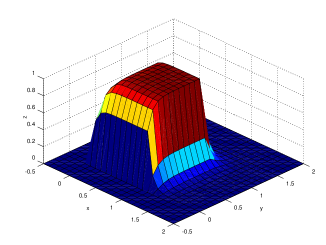
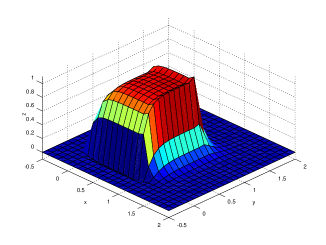
Figure 1: Numerical solutions of the linear two-dimensional problem after one time step with $v=1$ (left) satisfying the monotonicity condition and with $v=1.5$ (right), resulting in a monotonicity violation as in the one-dimensional case. The same behavior also occurs for velocities $1<v<1.5$, resulting in much less amplitudes of the violations.

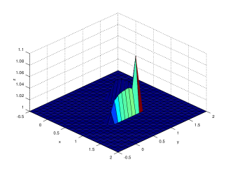
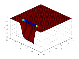
Figure 2: Plots showing in detail the monotonicity violation in the case $\Delta t=\Delta x=\Delta y=0.1$ and $v=1.5$, obtained after one time step with the implicit Lax-Friedrichs scheme: The maximum of $1.0$ and the numerical solution (left) and the minimum of $0.0$ and the numerical solution (right).

4.3 An implicit Godunov-type method

In the scalar case, a closed form of the exact solution of a Riemann-problem was described by Osher [16]. Using this, a numerical scheme can be defined via the $d$ numerical flux functions

$$g^{G}_{l}(v,w)\;=\;\left\{\begin{array}[]{ccc}\min_{v\leq u\leq w}f_{l}(u)&:&v\leq w\,,\\ \max_{w\leq u\leq v}f_{l}(u)&:&v>w\,.\end{array}\right.$$

Since the relative values of the test variables have to be compared within the scheme, diversions by cases have to be employed.
To condition (18):
Generally, for $l=1,\,\ldots,\,d$,

$$\tilde{H}_{l}(a+\Delta a,b,c)-\tilde{H}_{l}(a,b,c)=\frac{\Delta t}{\Delta x_{l}}\bigl{[}g_{l}^{G}(a+\Delta a,b)-g_{l}^{G}(a,b)\bigr{]}$$

holds. Since only the values $b,\,a$ and $a+\Delta a$ are of importance, it is necessary to investigate three cases for each $l\in\underline{d}$.

1. Case: $b\leq a\leq a+\Delta a$

   $$\frac{\Delta t}{\Delta x_{l}}\bigl{[}g_{l}^{G}(a+\Delta a,b)-g_{l}^{G}(a,b)\bigr{]}=\frac{\Delta t}{\Delta x_{l}}\left[\,\max_{b\leq u\leq a+\Delta a}f_{l}(u)-\max_{b\leq u\leq a}f_{l}(u)\,\right]\;\geq 0\,.$$

2. Case: $a\leq b\leq a+\Delta a$

   $$\frac{\Delta t}{\Delta x_{l}}\bigl{[}g_{l}^{G}(a+\Delta a,b)-g_{l}^{G}(a,b)\bigr{]}=\frac{\Delta t}{\Delta x_{l}}\left[\,\max_{b\leq u\leq a+\Delta a}f_{l}(u)-\min_{a\leq u\leq b}f_{l}(u)\,\right]\;\geq 0\,.$$

3. Case: $a\leq a+\Delta a\leq b$

   $$\frac{\Delta t}{\Delta x_{l}}\bigl{[}g_{l}^{G}(a+\Delta a,b)-g_{l}^{G}(a,b)\bigr{]}=\frac{\Delta t}{\Delta x_{l}}\left[\,\min_{a+\Delta a\leq u\leq b}f_{l}(u)-\min_{a\leq u\leq b}f_{l}(u)\,\right]\;\geq 0\,.$$

Thus, the validity of the condition (18) is guaranteed without any additional condition on the flux function. This can be verified analogously for condition (19), so that the investigated Godunov-type scheme is monotone for general continuous flux functions.

4.4 Convergence

Within this section, we prove convergence of the mentioned schemes under the assumption that the conditions for monotonicity are fulfilled. We do this in some detail for the implicit upwind method, since this is demonstrated in the easiest fashion, and we refer to the differences concerning the proofs of convergence with respect to the other methods afterwards. The same holds true with respect to the type of sources employed in Scenario 2. Since part of the convergence proof is technically identical to the proofs in the one-dimensional case without sources described in [3], we refer to that work for more details.

The basic idea of the convergence proofs is the following. Corresponding to sequences $\Delta x_{l}^{k}\downarrow 0$ for $k\to\infty$, $l\in\underline{d}$, we construct a monotonically growing sequence of discrete initial data. Then by the monotonicity of the method we get a monotonically growing sequence of numerical solutions. Since we multiply the initial function $u_{0}$ with an arbitrarily chosen but fixed test function with compact support, we only have to consider $u_{0}$ over a finite domain. Because of the assumption $u_{0}\in L_{\infty}$ and since we have $L_{\infty}$-Stability, the corresponding function sequence is integrable and bounded from above. Then we can use the well-known theorem of monotone convergence of Beppo Levi to show convergence (almost everywhere) to a limit function. More formally, we state the following

Theorem 4.1.

Let $u_{0}(\mathbf{x})$ be in $L^{loc}_{\infty}\left(\mathbb{R}^{d};\,\mathbb{R}\right)$. Consider a sequence of nested grids indexed by $k=1,2,\ldots$, with mesh parameters $\Delta t_{k}\downarrow 0$ and $\Delta x_{l}^{k}\downarrow 0$, $l=1,\,\ldots,\,d$, as $k\to\infty$, and let $u_{k}(\mathbf{x},t)$ denote the step function obtained via the numerical approximation by a consistent, conservative and monotone scheme in the form of the discussed methods. Then $u_{k}(\mathbf{x},t)$ converges to the unique entropy solution of the given conservation law as $k\to\infty$.

Proof.

At first, the convergence to a weak solution of the conservation law is established, followed by the verification that this weak solution is the entropy solution. For brevity of the notation, we omit the arguments $(\mathbf{x},t)$ when appropriate.

We employ sequences $\Delta t_{k}\downarrow 0$ and $\Delta x_{l}^{k}\downarrow 0$, assuming that the resulting grids are nested in order to compare data sets of values, i.e. refined grids always inherit cell borders.

The most important technical detail is the special discretization of the initial condition $u_{0}\in L^{loc}_{\infty}\left(\mathbb{R}^{d};\,\mathbb{R}\right)$. After a suitable modification on a set of Lebesgue measure zero, the initial condition is discretized on cell $j\in J$, i.e. for

$$\mathbf{x}\in\left((j_{1}-1)\Delta x_{1}^{0},j_{1}\Delta x_{1}^{0}\right]\times\ldots\times\left((j_{d}-1)\Delta x_{d}^{0},j_{d}\Delta x_{d}^{0}\right]\,,$$

by

$$u_{j}^{0}\;:=\;\inf_{\mathbf{x}\textrm{ in cell }j}u_{0}(\mathbf{x})\,.$$ (30)

Corresponding to the initial data we also define a piecewise continuous function

$$u_{k}(\mathbf{x},0):=u_{j}^{0}\textrm{, }\mathbf{x}\textrm{ in cell }j\,.$$ (31)

It is a simple matter of classical analysis to verify that the discretization (30) together with (31) gives on any compact spatial domain a monotonically growing function sequence with

$$\lim_{k\to\infty}u_{k}(\mathbf{x},0)\;=\;u_{0}(\mathbf{x})\textrm{ almost everywhere}$$ (32)

by application of the theorem of monotone convergence. In the classical fashion using point values, we extract discrete test elements $\phi_{j}^{0}$ out of a given test function $\phi\in C_{0}^{\infty}\left(\mathbb{R}^{d+1};\,\mathbb{R}\right)$. Additionally, we define for $n\geq 1$ the step function

$$u_{k}(x,t)=u_{j}^{n}\textrm{, }\mathbf{x}\textrm{ in cell }j\textrm{, }t^{n-1}<t\leq t^{n}\,.$$

In the following, let the test function $\phi$ be chosen arbitrarily but fixed.

Multiplication of the implicit upwind scheme (26) with $\Delta t^{k}\prod_{l=1}^{d}\Delta x_{l}^{k}$ as well as with the discrete test element $\phi_{j}^{n+1}$, summation over the spatial indices $j\in J$ and the temporal indices $n\geq 0$, and finally summation by parts yields

$$\Delta t^{k}\prod_{l=1}^{d}\Delta x_{l}^{k}\left\{\sum_{j\in J}\sum_{n\geq 0}\left[u_{j}^{n}\frac{\phi_{j}^{n+1}-\phi_{j}^{n}}{\Delta t^{k}}+\sum_{l=1}^{d}f_{l}(u_{j}^{n+1})\frac{\phi_{j+\delta l}^{n+1}-\phi_{j}^{n+1}}{\Delta x_{l}^{k}}\right]\right\}$$ (33)

$$= -\prod_{l=1}^{d}\Delta x_{l}^{k}\sum_{j\in J}u_{j}^{0}\phi_{j}^{0}+\Delta t^{k}\prod_{l=1}^{d}\Delta x_{l}^{k}\sum_{j\in J}q_{j}^{n+1}\phi_{j}^{n+1}\,.$$

By the definition of the introduced step functions, (33) is equivalent to

$$\int_{\mathbb{R}_{+}}\int_{\mathbb{R}^{d}}\left[u_{k}(\mathbf{x},t)\frac{\phi_{k}(\mathbf{x},t+\Delta t^{k})-\phi_{k}(\mathbf{x},t)}{\Delta t^{k}}\right.$$ (34)

$$+\left.\sum_{l=1}^{d}f_{l}(u_{k}(\mathbf{x},t+\Delta t^{k}))\frac{\phi_{k}(\mathbf{x}+\Delta x_{l}^{k},t+\Delta t^{k})-\phi_{k}(\mathbf{x},t+\Delta t^{k})}{\Delta x_{l}^{k}}\right]\,\mathrm{d}\mathbf{x}\,\mathrm{d}t$$

$$= -\int_{\mathbb{R}^{d}}u_{k}(\mathbf{x},0)\phi_{k}(\mathbf{x},0)\,\mathrm{d}\mathbf{x}+\int_{\mathbb{R}_{+}}\int_{\mathbb{R}^{d}}q_{k}(\mathbf{x},t+\Delta t^{k})\phi_{k}(\mathbf{x},t+\Delta t^{k})\,\mathrm{d}\mathbf{x}\,\mathrm{d}t\,.$$

We now prove convergence of (34) to the form which implies that $u$ is a weak solution of the original problem, see (7).

We first investigate the right hand side of (34). Set $\tilde{\Delta}:=\max_{l\in\underline{d}}\Delta x_{l}^{0}$ and let

$$K:=\left\{\,(\mathbf{x},t)\,|\,\exists(\mathbf{y},t)\in\mathrm{supp}(\phi):\,t=0\textrm{ and }y_{l}-\tilde{\Delta}\leq x_{l}\leq y_{l}+\tilde{\Delta}\textrm{ for all }l\in\underline{d}\,\right\}\,.$$

By construction, $K$ is compact and gives the largest possible spatial domain where non-zero discrete initial data may occur. Adding zeroes, we now cast the problem into a more suitable form, namely

$$\int_{\mathbb{R}^{d}}u_{k}(\mathbf{x},0)\phi_{k}(\mathbf{x},0)\,\mathrm{d}\mathbf{x}=\int_{K}u_{0}(\mathbf{x})\phi(\mathbf{x},0)\,\mathrm{d}\mathbf{x}$$ (35)

$$\quad+\int_{K}u_{k}(\mathbf{x},0)\left[\phi_{k}(\mathbf{x},0)-\phi(\mathbf{x},0)\right]\,\mathrm{d}\mathbf{x}+\int_{K}\left[u_{k}(\mathbf{x},0)-u_{0}(\mathbf{x})\right]\phi(\mathbf{x},0)\,\mathrm{d}\mathbf{x}\,.$$

Because of $u_{0}\in L^{\infty}(\mathbb{R}^{d};\,\mathbb{R})$ and by our construction, we can estimate the absolute value of the second right hand side term in (35) by the help of a constant $M_{u}<\infty$:

$$\left|\int_{K}u_{k}(\mathbf{x},0)\left[\phi_{k}(\mathbf{x},0)-\phi(\mathbf{x},0)\right]\,\mathrm{d}\mathbf{x}\right|\leq M_{u}\mathopen{|}K\mathclose{|}\sup_{x\in K}\left|\phi_{k}(\mathbf{x},0)-\phi(\mathbf{x},0)\right|\,.$$ (36)

Since $\phi$ is a smooth test function, it is a simple but technical exercise to show

$$\|\phi_{k}(\mathbf{x},0)-\phi(\mathbf{x},0)\|_{\infty}\to 0\quad\textrm{for}\quad k\to\infty\,.$$ (37)

By (36) and (37), the investigated term tends to zero with $k\to\infty$. Since $\phi$ is continuous and since $u_{k}(\mathbf{x},0)$ approaches $u_{0}(\mathbf{x})$ from below by construction, we can estimate the absolute of the third right hand side term in (35) with the help of a constant $M_{\phi}<\infty$ by

$$\left|\int_{K}\left[u_{k}(\mathbf{x},0)-u_{0}(\mathbf{x})\right]\phi(\mathbf{x},0)\,\mathrm{d}\mathbf{x}\right|\leq M_{\phi}\int_{K}u_{0}(\mathbf{x})-u_{k}(\mathbf{x},0)\,\mathrm{d}\mathbf{x}\,.$$

The theorem of monotone convergence implies that

$$\int_{K}u_{0}(\mathbf{x})-u_{k}(\mathbf{x},0)\,\mathrm{d}\mathbf{x}$$

vanishes in the limit for $k\to\infty$, i.e. the corresponding term in (35) goes to zero for $k\to\infty$. To condense these results, we obtain

$$\lim_{k\to\infty}\int_{\mathbb{R}^{d}}u_{k}(\mathbf{x},0)\phi_{k}(\mathbf{x},0)\,\mathrm{d}\mathbf{x}=\int_{\mathbb{R}^{d}}u_{0}(\mathbf{x})\phi(\mathbf{x},0)\,\mathrm{d}\mathbf{x}\,.$$

It remains to show

$$\int_{\mathbb{R}_{+}}\int_{\mathbb{R}^{d}}q_{k}(\mathbf{x},t+\Delta t^{k})\phi_{k}(\mathbf{x},t+\Delta t^{k})\,\mathrm{d}\mathbf{x}\,\mathrm{d}t\stackrel{{\scriptstyle k\to\infty}}{{\longrightarrow}}\int_{\mathbb{R}_{+}}\int_{\mathbb{R}^{d}}q(\mathbf{x},t)\phi(\mathbf{x},t)\,\mathrm{d}\mathbf{x}\,\mathrm{d}t\,.$$

This result can easily be achieved by analogously introducing a compact domain $S\subset\mathbb{R}^{d}$ including the support of $\phi$ in space and time, setting for $n\geq 1$ ($n=0$ is not relevant since $q(\cdot,0)\equiv 0$)

$$q_{j}^{n}\;:=\;\inf_{(\mathbf{x},t)\textrm{ with }\mathbf{x}\textrm{ in cell }j\textrm{ and $t$ in }\left(t^{n}-\Delta t^{0},t^{n}\right]}q(\mathbf{x},t)$$

and using a similar manipulation as for the terms involving $u_{0}$.

Concerning the left hand side of (35), adding zeroes and using the attributes of test functions together with the $L_{\infty}$-stability of $u_{k}$ yields that we finally have to show

$$\lim_{k\to\infty}\int_{S}\bigl{|}u(\mathbf{x},t)-u_{k}(\mathbf{x},t)\bigr{|}\left|\phi_{t}(\mathbf{x},t)\right|\,\mathrm{d}\mathbf{x}\,\mathrm{d}t\stackrel{{\scriptstyle k\to\infty}}{{\longrightarrow}}0$$ (38)

and also for all $l\in\underline{d}$

$$\lim_{k\to\infty}\int_{S}\bigl{|}f_{l}(u(\mathbf{x},t))-f_{l}(u_{k}(\mathbf{x},t+\Delta t^{k}))\bigr{|}\left|\frac{\partial}{\partial x_{l}}\phi(\mathbf{x},t)\right|\,\mathrm{d}\mathbf{x}\mathrm{d}t\stackrel{{\scriptstyle k\to\infty}}{{\longrightarrow}}0$$ (39)

in order to prove convergence to a weak solution. Since $\phi_{t}$ is continuous on $S$, we can estimate $\left|\phi_{t}\right|$ in (38) by a constant $M_{t}<\infty$. Since $u_{k}(\mathbf{x},t)$ grows monotonically with $k\to\infty$ in the sense of pointwise comparison, and since it is positive and bounded from above because of $u_{0}\in L_{\infty}(S)$ and the monotonicity of the method, the function sequence $\left(u_{k}(\mathbf{x},t)\right)_{k\in\mathbf{N}}$ converges almost everywhere to an integrable limit function on $S$ by the theorem of monotone convergence due to Levi. We set

$$u(\mathbf{x},t)\,:=\,\lim_{k\to\infty}u_{k}(\mathbf{x},t)\,.$$

Introducing exactly this limit function as the function $u(\mathbf{x},t)$ used up to now, the corresponding term in (38) becomes zero in the limit:

$$\lim_{k\to\infty}\int_{S}\bigl{|}u(\mathbf{x},t)-u_{k}(\mathbf{x},t)\bigr{|}\left|\phi_{t}(\mathbf{x},t)\right|\,\mathrm{d}\mathbf{x}\,\mathrm{d}t\leq M_{t}\int_{S}u(\mathbf{x},t)-\lim_{k\to\infty}u_{k}(\mathbf{x},t)\,\mathrm{d}\mathbf{x}\,\mathrm{d}t=0\,.$$

Note that the pointwise convergence $u_{k}\to u$ almost everywhere is now established and can be used in the following proofs. For proving (39), we need some further simple manipulations. We use again the continuity of the derivatives of $\phi$ to introduce constants $M^{l}_{x}<\infty$ to obtain

$$\int_{S}\bigl{|}f_{l}(u(\mathbf{x},t))-f_{l}(u_{k}(\mathbf{x},t+\Delta t^{k}))\bigr{|}\left|\frac{\partial}{\partial x_{l}}\phi(\mathbf{x},t)\right|\,\mathrm{d}\mathbf{x}\,\mathrm{d}t\leq$$ (40)

$$M^{l}_{x}\int_{S}\left|f_{l}(u_{k}(\mathbf{x},t))-f_{l}(u(\mathbf{x},t))\right|\,\mathrm{d}\mathbf{x}\,\mathrm{d}t$$

$$\;+M^{l}_{x}\int_{S}\left|f_{l}(u_{k}(\mathbf{x},t+\Delta t^{k}))-f_{l}(u_{k}(\mathbf{x},t))\right|\,\mathrm{d}\mathbf{x}\,\mathrm{d}t$$

for all $l\in\underline{d}$. We now discuss the first right hand side term in (40). Since by construction $u_{k}$ and $u$ are in $L_{\infty}(S)$, we can estimate every $\left|f_{l}(u_{k}(\mathbf{x},t+\Delta t^{k}))-f_{l}(u_{k}(\mathbf{x},t))\right|$ over $S$ from above by a constant $M^{l}_{f}<\infty$ because of the continuity of the $f_{l}$ on the compact set of possible values. Then the functions

$$M^{l}_{f}(\mathbf{x},t):=\left\{\begin{array}[]{ccc}M^{l}_{f}&,&(\mathbf{x},t)\in S\\ 0&,&\textrm{otherwise}\end{array}\right.\,,$$

are in $L_{1}(\mathbb{R}^{d}\times\mathbf{R_{+}};\,\mathbb{R})$ and dominate $\left|f_{l}(u_{k}(\mathbf{x},t))-f_{l}(u(\mathbf{x},t))\right|$ for all $l\in\underline{d}$ and all $k$. Because of the established pointwise convergence $u_{k}\to u$ a.e., we can apply the theorem of dominated convergence by Lebesgue to obtain for all $l$

$$\lim_{k\to\infty}M_{x}\int_{S}\left|f_{l}(u_{k}(\mathbf{x},t))-f_{l}(u(\mathbf{x},t))\right|\,\mathrm{d}\mathbf{x}\,\mathrm{d}t=0\,.$$ (41)

Now we discuss the second right hand side term in (40). Since by construction $u_{k}$ is a step function with finite values on the compact domain $S$, $u_{k}$ is in $L_{1}(S)$. Since the $f_{l}$ are continuous, also $f_{l}\circ u_{k}$ are in $L_{1}(S)$. By the continuity in the mean of $L_{1}$-functions, there exist $\delta_{l}(\epsilon)$ for all $\epsilon>0$ with

$$\int_{S}\left|f_{l}(u_{k}(\mathbf{x},t+\Delta t^{k}))-f_{l}(u_{k}(\mathbf{x},t))\right|\,\mathrm{d}\mathbf{x}\,\mathrm{d}t\,<\,\epsilon\,,$$

if $\Delta t^{k}<\delta_{l}(\epsilon)$. Since $\Delta t^{k}\downarrow 0$ for $k\to\infty$, $\epsilon$ can be chosen arbitrarily small, i.e.

$$M_{x}\int_{S}\left|f_{l}(u_{k}(\mathbf{x},t+\Delta t^{k}))-f_{l}(u_{k}(\mathbf{x},t))\right|\,\mathrm{d}\mathbf{x}\,\mathrm{d}t\,\to\,0\;\textrm{ for }\;k\to\infty$$ (42)

holds for all $l\in\underline{d}$. By (41) and (42) the assertion in (39) is proven. Since the test element $\phi$ was chosen arbitrarily, convergence to a weak solution is established.

We have now to show that exactly this weak solution is the unique entropy solution in the sense of Kružkov. Therefore, we derive in a similar fashion as in the derivation of (33) the weak form of the discrete entropy condition (21) connected with the implicit upwind scheme using Lemma 3.1 and Theorem 3.2. It reads

$$-\Delta t^{k}\prod_{l=1}^{d}\Delta x_{l}^{k}\sum_{j\in J}\mathopen{|}u_{j}^{0}-k\mathclose{|}\phi_{j}^{0}-\Delta t^{k}\prod_{l=1}^{d}\Delta x_{l}^{k}\sum_{j\in J}\sum_{n\geq 0}\mathrm{sgn}\left(u_{j}^{n+1}-k\right)q_{j}^{n+1}\phi_{j}^{n+1}$$ (43)

$$\leq \Delta t^{k}\prod_{l=1}^{d}\Delta x_{l}^{k}\sum_{j\in J}\sum_{n\geq 0}\left[\mathopen{|}u_{j}^{n}-k\mathclose{|}\frac{\phi_{j}^{n+1}-\phi_{j}^{n}}{\Delta t^{k}}\right.$$

$$\qquad+\mathrm{sgn}\left(u_{j}^{n+1}-k\right)\sum_{l=1}^{d}\left\{\left[f_{l}(u_{j}^{n+1})-f_{l}(k)\right]\frac{\phi_{j+1}^{n+1}-\phi_{j}^{n+1}}{\Delta x_{l}^{k}}\right\}\Biggr{]}\,.$$

Using the established convergence $u_{k}\to u$ a.e. of the function sequence generated by the numerical method for $\Delta t^{k}\downarrow 0$ and $\Delta x_{l}^{k}\downarrow 0$ for all $l\in\underline{d}$, we now prove convergence of (43) towards the form of the entropy condition due to Kružkov (2). Therefore, we have to consider arbitrarily chosen but fixed test elements composed of a test function $\phi$ with $\phi\geq 0$, $\phi\in C_{0}^{\infty}(\mathbb{R}^{d+1};\,\mathbb{R})$, and a test number $k\in\mathbb{R}$.

Using the same notation and applying a similar procedure as in the case of the convergence proof to a weak solution, we first want to prove

$$\lim_{k\to\infty}M_{\phi}\int_{K}\bigl{|}\left|u_{k}(\mathbf{x},0)-k\right|-\left|u_{0}(\mathbf{x})-k\right|\bigr{|}\,\mathrm{d}\mathbf{x}=0\,.$$ (44)

Since $k$ is fixed and $u_{k}(\mathbf{x},0)$ and $u_{0}$ bounded, one can find a constant function over the compact interval $K$ which dominates the integrand for all $k$. Then (44) follows by the use of the already established convergence $u_{k}(x,0)\to u_{0}(x)$ a.e. and the theorem of dominated convergence by Lebesgue. We also have to treat

$$\lim_{k\to\infty}\int_{\mathbb{R}_{+}}\int_{\mathbb{R}^{d}}\mathrm{sgn}\left(u_{k}(\mathbf{x},t+\Delta t^{k})-k\right)q_{k}(\mathbf{x},t+\Delta t^{k})\phi(\mathbf{x},t+\Delta t^{k})\,\mathrm{d}\mathbf{x}\,\mathrm{d}t\,.$$

Therefore, we expand the factor $\phi(\mathbf{x},t+\Delta t^{k})$ by adding zeroes in the form

$$\phi(\mathbf{x},t+\Delta t^{k})=\phi(\mathbf{x},t+\Delta t^{k})-\phi(\mathbf{x},t)+\phi(\mathbf{x},t)\,.$$

Convergence of the integrals involving the factor $\phi(\mathbf{x},t+\Delta t^{k})-\phi(\mathbf{x},t)$ tend to zero. This follows by estimating $\mathrm{sgn}$, $u_{k}$ and $q_{k}$ from above and using the usual properties of test functions. In a similar fashion, we expand the factor $\mathrm{sgn}\left(u_{k}(\mathbf{x},t+\Delta t^{k})-k\right)$, adding zero in the form $-\mathrm{sgn}\left(u_{k}(\mathbf{x},t)-k\right)+\mathrm{sgn}\left(u_{k}(\mathbf{x},t)-k\right)$. The proof that the integrals involving $\mathrm{sgn}\left(u_{k}(\mathbf{x},t+\Delta t^{k})-k\right)-\mathrm{sgn}\left(u_{k}(\mathbf{x},t)-k\right)$ vanish follows from the continuity in the mean of $L_{1}$-functions. Again similarly, we expand in the form $q_{k}(\mathbf{x},t+\Delta t^{k})=q_{k}(\mathbf{x},t+\Delta t^{k})-q(\mathbf{x},t+\Delta t^{k})+q(\mathbf{x},t+\Delta t^{k})$ and use the concept of monotone convergence due to Beppo Levi to obtain convergence to zero of the integrals involving $q_{k}(\mathbf{x},t+\Delta t^{k})-q(\mathbf{x},t+\Delta t^{k})$. Lastly, the proof of convergence of $q(\mathbf{x},t+\Delta t^{k})$ to $q(\mathbf{x},t)$ under the integral follows from the continuity in the mean of $L_{1}$-functions. The technical details only require to take all expansions obtained by taking suitable zeroes into account and eliminating all integrals which involve discrete notions. The other terms left to investigate are

$$\int_{S}\left|u_{k}(\mathbf{x},t)-k\right|\phi_{t}(\mathbf{x},t)\,\mathrm{d}\mathbf{x}\,\mathrm{d}t\quad\textrm{and}$$

$$\int_{S}\sum_{l=1}^{d}\mathrm{sgn}\left[u_{k}(\mathbf{x},t+\Delta t^{k})-k\right]\bigl{[}f_{l}(u_{k}(\mathbf{x},t+\Delta t^{k}))-f_{l}(k)\bigr{]}\frac{\partial}{\partial x_{l}}\phi(\mathbf{x},t)\,\mathrm{d}\mathbf{x}\,\mathrm{d}t\,.$$

The procedure is the same in both cases. Since the occurring derivatives of $\phi$ are continuous, we can estimate these over the compact domain $S$ by finite constants. Since $k$ is a fixed value (and so is $f_{l}(k)$ for all $l\in\underline{d}$), since $u_{k}(\mathbf{x},t)$ is bounded and because the $f_{l}$ are continuous over the bounded interval of possible values of $u_{k}$ (due to the established $L_{\infty}$-stability), we can also give constants which estimate all the expressions involving $u_{k}$ from above. Using the product of these finite constants as dominating function over $S$ as well as $u_{k}\to u$ a.e., we employ the theorem of dominated convergence to receive the desired result for the implicit upwind scheme.

In the case of the implicit Lax-Friedrichs method, we have to assume Lipschitz continuity with a Lipschitz constant $L\leq 1/\lambda$ of the flux functions so that the method is monotone. In comparison to the implicit upwind method, the difference in the corresponding weak forms are made up from

$$-\frac{\Delta t_{k}}{2}\int_{S}u_{k}(\mathbf{x},t+\Delta t^{k})\hat{\phi}\,\mathrm{d}\mathbf{x}\,\mathrm{d}t\textrm{ and }-\frac{\Delta t_{k}}{2}\int_{S}\left|u_{k}(\mathbf{x},t+\Delta t^{k})-k\right|\hat{\phi}\,\mathrm{d}\mathbf{x}\,\mathrm{d}t\,,$$

respectively. Thereby, $\hat{\phi}$ converges in the $L_{\infty}$-Norm to $\partial^{2}_{x_{l}^{2}}\phi(\mathbf{x},t)$ which is continuous since $\phi\in C_{0}^{\infty}(\mathbb{R}^{d+1};\,\mathbb{R})$. Thus, the corresponding term can be estimated from above by a constant over the compact domain $S$. Since $k$ is fixed and $u_{k}(\mathbf{x},t)$ is bounded as usual, both expressions vanish with $\Delta t^{k}\downarrow 0$.

With respect to the described implicit Godunov-type method, we use a similar procedure as in the case of the implicit Lax-Friedrichs methods, namely to write down the differences in the weak forms to the case of the implicit upwind method. These are made up from

$$\Bigl{\{}\bigl{[}g_{l}^{G}(u_{j}^{n+1}\vee k,u_{j+\delta l}^{n+1}\vee k)-g_{l}^{G}(u_{j}^{n+1}\wedge k,u_{j+\delta l}^{n+1}\wedge k)\bigr{]}\Bigr{.}$$

$$\quad\Bigl{.}-\mathrm{sgn}\left(u_{j}^{n+1}-k\right)\bigl{[}f_{l}(u_{j}^{n+1})-f_{l}(k)\bigr{]}\Bigr{\}}\frac{\phi_{j+\delta l}^{n+1}-\phi_{j}^{n+1}}{\Delta x_{l}^{k}}$$ (45)

$$\textrm{and}\quad\bigl{[}g_{l}^{G}(u_{j}^{n+1},u_{j+1}^{n+1})-f_{l}(u_{j}^{n+1})\bigr{]}\frac{\phi_{j+\delta l}^{n+1}-\phi_{j}^{n+1}}{\Delta x_{l}^{k}}\,.$$ (46)

Since $g_{G}$ is continuous in the components and $u_{k}(\mathbf{x},t)\in L_{1}(S)$, the $g_{l}^{G}\circ u_{k}$ are also in $L_{1}(S)$. After introducing step functions as usual, the expressions incorporating $g_{l}^{G}$ from (45) give values $f_{l}(\xi_{l})$ with

$$\begin{array}[]{cc}&\xi_{l}\in\left[u_{k}(\mathbf{x},t+\Delta t^{k}),u_{k}(\mathbf{x}+\Delta x_{l}^{k},t+\Delta t^{k})\right]\\ \textrm{or}&\;\xi_{l}\in\left[u_{k}(\mathbf{x}+\Delta x_{l}^{k},t+\Delta t^{k}),u_{k}(\mathbf{x},t+\Delta t^{k})\right]\,,\end{array}$$

respectively. The integrals over the terms corresponding to (45) then go to zero with $k\to\infty$ because of the continuity in the mean of $g_{l}^{G}\circ u_{k}$. The idea for proving convergence to zero concerning the integral of the expressions corresponding to (46) is the same.

Concerning Scenario 2, the described strategy is fully transferable by employing accordingly the notions developed in section 3. ∎

5 Numerical tests

In order to show the applicability of the developed notions, we investigate numerically a number of test cases which were employed within the literature in various contexts. In contrast to the cited examples from [17, 9] we do not employ any further manipulations of the problem or on the numerical side, we simply rely on the straightforward application of the implicit Godunov-type method in all cases.

We remark that the notions we developed reduce in the one-dimensional case without sources to the notions described within [2, 3]. In that works, especially the applicability of implicit schemes with respect to a conservation law given in [12] was shown where the solution features a rarefaction wave extending in an arbitrarily small time step to infinity. Thus, the applicability of the described concept is already established in the case without sources, where the flux is merely continuous and where a meaningful CFL-condition does not exist. With the numerical tests documented in this section, we focus on the theoretical extensions developed in this paper.

First, we employ a one-dimensional conservation law featuring as a particular problem a point source depending on space and time. This test case was used in [17] to show experimentally convergence to the entropy solution. In contrast to the scheme used in their work, for our scheme convergence to the entropy solution is guaranteed.

At second, we consider a couple of model problems featuring spatial dependent sources having the form of the derivative of certain functions. These model problems were used in [9] in order to show numerically convergence to steady state solutions featuring various difficulties which is in contrast to the first unsteady example. Moreover, since we use the described Godunov-type scheme, we do not rely on a CFL-like condition as in [9] which greatly restricts the time step size, an annoying aspect in steady state calculations. Note also that we simply employ the described implicit method without any further improvements as done with the explicit method employed in [9] for which convergence was not guaranteed.

While the first two examples could be identified as belonging to Scenario 1, the third test case refers to Scenario 2. It consists of a one-dimensional model problem featuring a parameter dependent source term depending also in a nonlinear way on the solution. This model problem was used by LeVeque and Yee [15] to illuminate numerical difficulties in the case of stiffness.

As fourth and last example, we show numerical results of a two-dimensional problem used in [8] which exhibits all principal difficulties encountered when dealing with hyperbolic equations. As in the second example, the implicitness of our methods is advantageous in order to calculate the steady state solution.

In all examples, nonlinear systems of equations arise which have been solved numerically with an iterative solver. Precisely, we used the MINPACK subroutine hybrd.

Example 1

The one-dimensional scalar conservation law under consideration is

$$\frac{\partial}{\partial t}u(x,t)+\frac{\partial}{\partial x}u(x,t)=\sin(\pi t)\delta(x-0.1)\,,\quad x\in(0,1)\,,\;t>0\,,$$

$$\textrm{with}\quad u_{0}(x)=u(x,0)=0\;\forall x\in(0,1)\quad\textrm{and}\quad u(0,t)=0\;\forall t\geq 0\,.$$

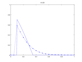
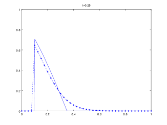
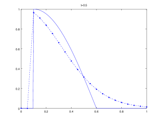
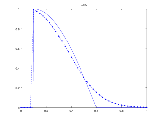
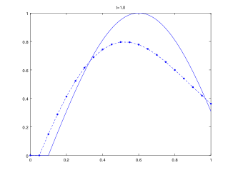
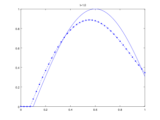
Figure 3: The columns show the numerical solutions (dashed lines) in comparison with the exact solution (continuous lines). The situations displayed in the right column are obtained using a grid twice as fine as in the left column.

The exact solution is given in [17] and reads

$$u(x,t)\;=\;\left\{\begin{array}[]{ccc}u_{0}(x-t)&:&x<0.1\textrm{ or }x\geq 0.1+t\,,\\ \sin\left(\pi(0.1+t-x)\right)+u_{0}(x-t)&:&0.1\leq x<0.1+t\,.\end{array}\right.$$

By Figure 3, we can compare the exact and numerical solutions obtained with the implicit upwind method in the same situations as displayed in [17], using also exactly the same grid parameters. They used $\Delta x=\Delta t=1/20$ and $\Delta x=\Delta t=1/40$ in the three moments $t=1/4$, $t=1/2$, and $t=1$.

Relating to the method used in [17], our scheme is overall much more viscous. This is as expected since Santos and Oliveira especially sought a good accuracy of their method. We also observe experimentally convergence to the correct solution by our method, documented by the bottom pictures within Figure 4 showing results of analogous computations with a more refined grid.

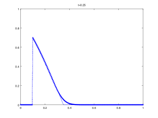
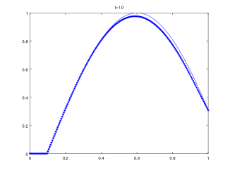
Figure 4: The first and third state from Figure 3 revisited, this time obtained via numerical approximation using a grid ten times as fine as in the left column of Figure 3.

Example 2

The conservation law generally under consideration is

$$\frac{\partial}{\partial t}u(x,t)+\frac{\partial}{\partial x}\left(\frac{1}{2}u(x,t)^{2}\right)=q_{x}(x)\,,\quad x\in\mathbb{R}\,,\;t>0\,,$$

which is used featuring different sources and initial conditions resulting in various difficulties. The source terms in use are

$$q(x)=\left\{\begin{array}[]{cc}0\,,&x<-1\,,\\ \cos^{2}\left(\pi x/2\right)\,,&-1\leq x\leq 1\,,\\ 0\,,&1<x\end{array}\right.\;\textrm{and}\;q(x)=\left\{\begin{array}[]{cc}0\,,&x<-1\,,\\ -\cos^{2}\left(\pi x/2\right)\,,&-1\leq x\leq 1\,,\\ 0\,,&1<x\,.\end{array}\right.$$

The initial conditions in use are

$$u(x,0^{+})=0,\qquad-\infty<x<\infty\,,\qquad u(x,0^{+})=\left\{\begin{array}[]{cc}0\,,&x<-1\,,\\ 1\,,&-1\leq x\leq 1\,,\\ 0\,,&1<x\,,\end{array}\right.\;\textrm{and}$$

$$u(x,0^{+})=\left\{\begin{array}[]{cc}0\,,&x<-1\,,\\ -1\,,&-1\leq x\leq 1\,,\\ 0\,,&1<x\,.\end{array}\right.$$

The following four experiments are analogous to the ones in [9], using exactly the same grid parameters as initially in [9] where later on spatial regridding was used in order to obtain sharp shock profiles. We use the implicit Lax-Friedrichs method with $\delta x=0.025$ and $\delta t=0.0125$.

In the Figures 5 and 6, we show in all test cases from top to bottom the numerical solutions obtained by using our method at times $t=0.2,\,0.5,\,1.0$ and $3.0$ (line featuring small circles) together with the stationary solution (continuous line). Thereby, different experiments correspond to different columns of pictures.

Concerning the first experiment, the numerical solution is almost identical to the exact one except at the point $x=0.0$ where a grid point is located exactly on the shock front. With respect to the other experiments, the numerical solutions exhibit slightly smeared shocks while they are otherwise quite accurate. Comparing with the numerical results shown in [9], not employing a regridding procedure results in slightly smeared shocks. Further numerical experiments have shown that we can employ much larger time steps — usually of about $20$–$30$ times the one used for the presented experiments — without degrading our numerical solution.

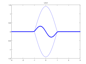
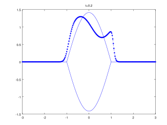
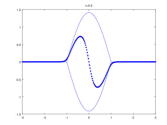
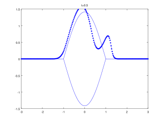
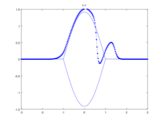
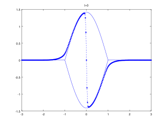
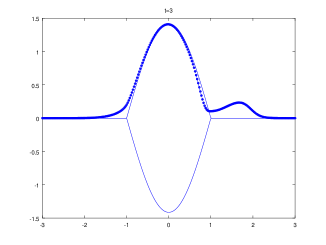
Figure 5: Experiments one (left) and two (right).

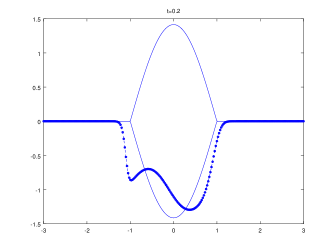
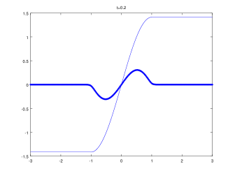
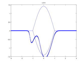
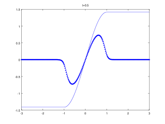
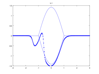
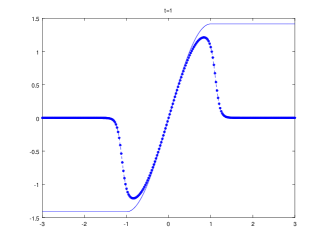
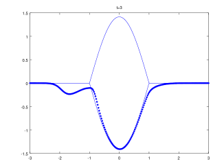
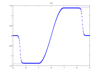
Figure 6: Experiments three (left) and four (right).

Example 3

The conservation law under consideration is

$$\frac{\partial}{\partial t}u(x,t)+\frac{\partial}{\partial x}u(x,t)=-\mu u(x,t)\bigl{(}u(x,t)-1\bigr{)}\left(u(x,t)-\frac{1}{2}\right)$$

which exhibits a nonlinear source term with an increasingly stiff behavior for $\mu$ growing large.

Our numerical investigations are completely analogous to the ones in [15]. The experiments consist of the numerical solution of a Riemann problem whose exact solution features a shock front moving from $x=0.3$ to $x=0.6$ after a couple of time steps, see Figure 7. For small and medium $\mu$, the numerical solution shows the correct behavior incorporating numerical viscosity; note the sharpening and slight translation of the shock approximation for $\mu=100$, an effect of the increasing stiffness of the source term. For $\mu=1000$ the usual problem is faced, see [15] for details. This experiment shows that although the discussed methods are generally capable to deal with non-linear sources, they are not recommended without modification for stiff problems even though they are fully implicit. Of course, grid refinement results in the approximation of the correct solution as expected.

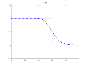
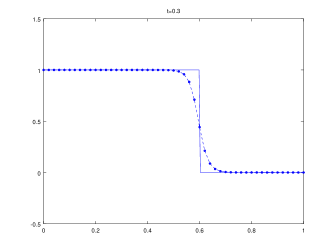
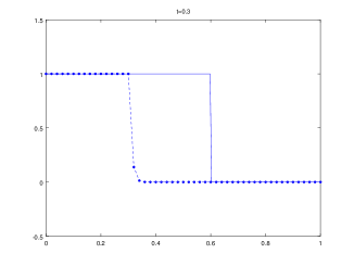
Figure 7: Numerical solutions (dashed lines) compared with the exact solution (continuous lines). The pictures correspond from left to right and top to bottom to the choices $\mu=1,10,100,1000$.

6 Summary and conclusive remarks

In this paper, we have introduced a new concept for implicit methods for scalar conservation laws in one or more spatial dimensions which may also include source terms of different type. We developed implicit notions that are centered around a monotonicity criterion and show the relation between a numerical scheme and a discrete entropy inequality. We investigate in detail three implicit methods and give a convergence proof. Hence, we extend the rigorously verified range of applicability of those three implicit numerical methods. By numerical experiments we have shown the validity and usefulness of our theoretical results.

References

• [1] P. Bénilan and S. Kružkov. Conservation laws with continuous flux functions. Nonlinear Differential Equations and Applications NoDEA, 3(4):395–419, 1996.
• [2] M. Breuß. Numerical Methods for Conservation Laws in Non-Standard-Situations. Doctoral thesis, University of Hamburg, 2001.
• [3] M. Breuß. The implicit upwind method for 1-d scalar conservation laws with continuous fluxes. SIAM J. Numer. Anal., 43(3):970–986, 2005.
• [4] F. Coquel and P. Le Floch. Convergence of finite difference schemes for conservation laws in several space dimensions: A general theory. SIAM Journal on Numerical Analysis, 30(3):675–700, 1993.
• [5] M. G. Crandall and A. Majda. Monotone difference approximations for scalar conservation laws. Mathematics of Computation, 34(149):1–21, 1980.
• [6] R. J. DiPerna. Measure-valued solutions to conservation laws. Archive for Rational Mechanics and Analysis, 88(3):223–270, 1985.
• [7] E. Godlewski and P.-A. Raviart. Hyperbolic systems of conservation laws. Collection Mathématiques et Applications de la SMAI. Ellipses, Paris, 1991.
• [8] T. Grahs, A. Meister, and T. Sonar. Image processing for numerical approximations of conservation laws: Nonlinear anisotropic artificial dissipation. SIAM Journal on Scientific Computing, 23(5):1439–1455, 2002.
• [9] J. M. Greenberg, A. Y. LeRoux, R. Baraille, and A. Noussair. Analysis and approximation of conservation laws with source terms. SIAM Journal on Numerical Analysis, 34(5):1980–2007, 1997.
• [10] S. N. Kružkov. First order quasilinear equations in several independent variables. Mathematics of the USSR-Sbornik, 10(2):217–243, 1970.
• [11] S. N. Kružkov and F. Hildebrand. The cauchy problem for quasilinear first order equations in the case the domain of dependence on initial data is infinite. Moscow Univ. Math. Bull., 29(5):75–81, 1974.
• [12] S. N. Kružkov and E. Y. Panov. Conservative quasilinear first-order laws with an infinite domain of dependence on the initial data. Soviet Math. Doklady, 42:316–321, 1991.
• [13] N. N. Kuznetsov. Accuracy of some approximate methods for computing the weak solutions of a first order quasi-linear equation. USSR Comp. Math. and Math. Phys., 16(6):105–119, 1976.
• [14] R. J. LeVeque. Numerical Methods for Conservation Laws. Lectures in Mathematics ETH Zürich, Department of Mathematics Research Institute of Mathematics. Birkhäuser Verlag, Basel, 1992.
• [15] R. J. Leveque and H. C. Yee. A study of numerical methods for hyperbolic conservation laws with stiff source terms. Journal of Computational Physics, 86(1):187–210.
• [16] S. Osher. Riemann solvers, the entropy condition, and difference approximations. SIAM Journal on Numerical Analysis, 21(2):217–235, 1984.
• [17] J. Santos and P. de Oliveira. A converging finite volume scheme for hyperbolic conservation laws with source terms. Journal of Computational and Applied Mathematics, 111(1–2):239–251, 1999.