An analytical method for error analysis of GRACE-like missions based on spectral analysis

Abstract

The aim of this paper is to present an analytical relationship between the power spectral density of GRACE-like mission measurements and the accuracies of the gravity field coefficients mainly from the point of view of theory of signal and system, which indicates the one-to-one correspondence between spherical harmonic error degree variances and frequencies of the measurement noise. In order to establish this relationship, the average power of the errors due to gravitational acceleration difference and the relationship between perturbing forces and range-rate perturbations are derived, based on the orthogonality property of associated Legendre functions and the linear orbit perturbation theory, respectively. This method provides a physical insight into the relation between mission parameters and scientific requirements. By taking GRACE-FO as the object of research, the effects of sensor noises and time variable gravity signals are analyzed. If LRI measurements are applied, a mission goal with a geoid accuracy of 7.4 cm at a spatial resolution of 101 km is reachable, whereas if the KBR measurement error model is applied, a mission goal with a geoid accuracy of 10.2 cm at a spatial resolution of 125 km is reachable. Based on the discussion of the spectral matching of instrument accuracies, an improvement in accuracy of accelerometers is necessary for the match between the range errors and accelerometer noises in the future mission. Temporal aliasing caused by the time variable gravity signals is also discussed by this method.

1 Introduction

The last dedicated gravity satellite missions like CHAMP, GRACE, GOCE and GRAIL have mapped the Earth’s and Moon’s gravity field with unprecedented high accuracy and resolution in the past decades (Reigber et al. 2002; Tapley et al. 2004; Rummel et al. 2011; Zuber et al. 2013). CHAMP and GOCE are mainly based on satellite-to-satellite tracking in the high-low mode (HL-SST) and satellite gravity gradiometry (SGG) respectively, while both GRACE and GRAIL satellite-to-satellite tracking use the low-low mode (LL-SST). Compared to HL-SST and SGG configurations, the LL-SST observations can derive the long wavelength components of the Earth’s gravity field with higher accuracy and map their variability in time in an efficient way. LL-SST missions based on intersatellite ranging may achieve significant improvements in spatial resolution and accuracy of gravity field model by using interferometric laser ranging instead of microwave ranging. Due to these advantages, the proposed future missions, like the GRACE Follow-On (GRACE-FO) (Flechtner et al. 2015), Next-Generation Gravity Mission (NGGM) (Cesare and Sechi 2013) concept and Earth System Mass Transport Mission (e.motion) proposal (Gruber et al. 2014), are all based on LL-SST configuration. Until now there exist four basic types of LL-SST satellites formations for the missions to choose from, i.e. collinear tandem (GRACE-like), pendulum, Cartwheel and LISA-type formation (c.f. Elsaka et al. 2014). Several studies were published to investigate the performance of these satellite formations, e.g. by Sharifi et al. (2007), Sneeuw et al. (2008), Wiese et al. (2009), Massotti et al. (2013), Elsaka et al. (2014) and Elsaka et al. (2015).

The upcoming GRACE-FO mission based on the collinear tandem configuration is about to be launched in 2017 and will have a nominal life-time of 7 years (Flechtner et al. 2014). By taking advantages of GRACE and GRAIL heritage, the GRACE-FO mission will continue to obtain the global models of the Earth’s time-variable gravity field, while on the other hand it will try to improve the LL-SST measurement performances. For this purpose, a 50-100 nm precise laser ranging interferometer (LRI) is included into the GRACE-FO payload as a science demonstrator instrument, which supplements the $\mu$m-level accuracy K-band ranging system (KBR). The GRACE-FO mission is expected to provide meaningful guidance to the future gravity satellite missions of LL-SST type after GRACE-FO.

The pre-mission error analysis is a key issue for the future mission design, which concerns the field where geodesy is in contact with physics and technical sciences. It allows one to determine the science requirements and parameters of missions before launch. The conventional error analysis and recovery methods of LL-SST are based on orbit perturbation theory or the principle of energy conservation in establishing the observation equations, which are generally solved by using least-squares (LS) theory (Colombo 1984; Touboul et al. 1999; Tapley et al. 2004). However, there was no one-to-one correspondence between spherical harmonics and frequencies in the measurements (Inácio et al. 2015), i.e. accelerometer data, range-rate data. That means the conventional methods estimate the individual effects of parameters and noise are too complicated to be described analytically since these methods address the effect of measurement errors mainly from a numerical point of view (Migliaccio et al. 2004; Cai et al. 2012).

By applying the theory of signal and system, this paper provides an analytical relationship between the power spectral density (PSD) of LL-SST measurements and the accuracies of gravity field coefficients, which indicates the one-to-one correspondence between spherical harmonic error degree variances and frequencies of the measurement noise. This error analysis method allows us to efficiently evaluate the science requirements and parameters of the missions. It is a helpful tool for identifying the frequency characteristics of signals in future gravity missions.

Sneeuw (2000) and Kim (2000) developed their respective semi-analytical theory on error analysis with different principles. The semi-analytical approach established by Sneeuw (2000) obtains the 2-D Fourier spectrum first by Fourier analysis and then transforms the Fourier coefficients into the spherical harmonic coefficients. In the latter step, the relationship between spherical harmonics and 2-D Fourier spectrum cannot be analytically given and must be preceded with applying least-squares. The semi-analytical method for degree error prediction established by Kim (2000) can obtain degree error variance of the gravity by a expression when that of range-rate is available. But before this step, the range-rate measurement noises due to various error sources need to be covered the entire sphere with the same latitude and longitude lengths and then mapped from the space domain into the spectral domain to obtain the degree variance of range-rate. These works made a significant contribution to the progress of efficient computation of error analysis of gravity field, however, these methods cannot lead to directly evaluate the frequency characteristics of measurement noise which affects spherical harmonic coefficient recovery due to the lack of analytical expression.

This paper, with GRACE-FO as the object of the research, discusses an analytical error analysis method of LL-SST (a collinear tandem configuration), and is organized as follows. In Sect. 2, the forces variation relationship between two satellites produced by the gravitational and non-gravitational accelerations is derived based on dynamic analysis of the satellite. The information of the range-rate is put in relation with the differential effect of the resultant forces acting on the twin satellites, which consist of gravitational terms, due to the gravity field of the Earth and third bodies, and non-gravitational terms, due to the surface forces like atmospheric drag and solar radiation. A direct analytical expression for the error analysis of LL-SST is then concluded based on the dynamic analysis and spectral analysis in Sect. 3. The transfer function between satellite perturbing forces and the range-rate are deduced in detail in Sects. 4. In Sect. 5, the effects of sensor noise and their matching together with temporal aliasing from both non-tidal and tidal sources on gravity field recovery are explicitly and quantitatively discussed by taking the advantage of this method.

2 Dynamic analysis

The fundamental relation of the LL-SST is the forces variation between two satellites produced by the gravitational and non-gravitational accelerations, which can be expressed in the inertial frame

$$\mathrm{\Delta}\mathord{\buildrel{\lower 3.0pt\hbox{$\scriptscriptstyle\rightharpoonup$}}\over{a}}=\mathrm{\Delta}\mathord{\buildrel{\lower 3.0pt\hbox{$\scriptscriptstyle\rightharpoonup$}}\over{g}}+\mathrm{\Delta}{\mathord{\buildrel{\lower 3.0pt\hbox{$\scriptscriptstyle\rightharpoonup$}}\over{a}}_{ng}},$$ (1)

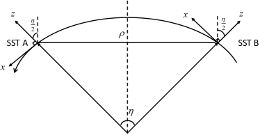
Figure 1: Configuration of two collinear tandem satellites

where $\mathrm{\Delta}\mathord{\buildrel{\lower 3.0pt\hbox{$\scriptscriptstyle\rightharpoonup$}}\over{a}}$ is the total acceleration perturbation difference between the satellites, $\mathrm{\Delta}\mathord{\buildrel{\lower 3.0pt\hbox{$\scriptscriptstyle\rightharpoonup$}}\over{g}}$ and $\mathrm{\Delta}{\mathord{\buildrel{\lower 3.0pt\hbox{$\scriptscriptstyle\rightharpoonup$}}\over{a}}_{ng}}$ are the gravitational acceleration perturbation difference and non-gravitational one, respectively. The total acceleration perturbation difference $\mathrm{\Delta}\mathord{\buildrel{\lower 3.0pt\hbox{$\scriptscriptstyle\rightharpoonup$}}\over{a}}$ can be determined from the range-rate measurements based on the perturbation theory. The gravitational accelerations are the strongest forces acting on the satellites and mainly determine the orbits, which are directly related to the distance between two satellites. In this study we focus on the effects of measurement errors on the Earth s gravity field recovery, therefore we ignore the accelerations acting on the low-flying satellite caused by the third bodies, such as the Moon, the Sun and other celestial bodies. The non-gravitational accelerations also have a significant impact on the satellite which are measured by an on-board accelerometer, although they are smaller than the gravitational ones. The acceleration perturbation difference with respect to local orbital reference frames shown in Fig. 1, which correspond to the along-track, cross-track and radial directions of each satellite (Mackenzie and Moore 1997), are provided as follows:

$$\left\{{\begin{array}[]{*{20}{c}}{\Delta{a_{x}}=\Delta{g_{x}}+\Delta{a_{x,ng}}}\\ {\Delta{a_{y}}=\Delta{g_{y}}+\Delta{a_{y,ng}}}\\ {\Delta{a_{z}}=\Delta{g_{z}}+\Delta{a_{z,ng}}}\end{array}}\right.,$$ (5)

where $\mathrm{\Delta}{a_{x}}$, $\mathrm{\Delta}{a_{y}}$ and $\mathrm{\Delta}{a_{z}}$ are the total acceleration perturbation differences in the along-track, cross-track and radial directions, respectively; $\mathrm{\Delta}{g_{x}}$, $\mathrm{\Delta}{g_{y}}$ and $\mathrm{\Delta}{g_{z}}$ are the gravitational ones; $\mathrm{\Delta}{a_{x,ng}}$, $\mathrm{\Delta}{a_{y,ng}}$ and $\mathrm{\Delta}{a_{z,ng}}$ are non-gravitational ones. In Fig. 1 $\eta$ and $\rho$ are the satellite separation and the intersatellite distance. Under the assumption of a perfect polar circular orbit in this study, the local north-oriented coordinate system is the same as the local orbital coordinate system. The range-rate perturbations come from the along-track and radial perturbation difference, while cross-track perturbation does not show up in this configuration with both satellites flying on the same nominal orbit (Sneeuw 2000). As a result, we shall deal with the along-track and radial components in this study. For the sake of clarity, Eq. (5) is rewritten as

$$\left\{{\begin{array}[]{*{20}{c}}{\Delta{g_{x}}=\Delta{a_{x}}-\Delta{a_{x,ng}}}\\ {\Delta{g_{z}}=\Delta{a_{z}}-\Delta{a_{z,ng}}}\end{array}}\right.,$$ (8)

From Eq. (8) it can be seen that the accuracy of the retrieved gravitational accelerations, which are the first order derivative of the gravitational potential, depends on the ranging system and accelerometer noises. The next section presents the relationship between measurement noises and the accuracies of gravity field coefficients based on the above acceleration equations.

3 Measurement noise and accuracies of gravity field coefficients

The disturbance gravitational potential of the Earth is a harmonic function and can be expanded into a series of spherical harmonics, depending on the spherical coordinates $r$, $\theta$ and $\lambda$ (Heiskanen and Moritz 1967)

$$T(r,\theta,\lambda) = \frac{GM}{R}\sum_{l=2}^{\infty}\left(\frac{R}{r}\right)^{l+1}\sum_{m=0}^{l}\bar{P}_{lm}\left(\cos{\theta}\right)\times$$ (9)

$${}\left(\bar{C}_{lm}\cos{m\lambda}+\bar{S}_{lm}\sin{m\lambda}\right),$$

where

$r,\theta,\lambda$ are geocentric spherical coordinates (radius, co-

latitude, longitude);

$R$ is reference length (mean semi-major axis of the Ea-

rth);

$GM$ is gravitational constant times mass of the Earth;

$l,m$ are degree, order of spherical harmonic;

$\bar{P}_{lm}\left(\cos{\theta}\right)$ are the fully normalized Legendre functi-

ons, and result in the relation $\displaystyle\frac{1}{4\pi}\int_{\sigma}\bar{P}_{lm}(\cos\theta)^{2}\times$

$\left(\begin{array}[]{c}\cos m\lambda\\ \sin m\lambda\end{array}\right)^{2}\mathrm{d}\sigma=1$, where $\displaystyle\int_{\sigma}\mathrm{d}\sigma$ means integration

on the unit sphere;

$\bar{C}_{lm},\bar{S}_{lm}$ are fully normalized potential coefficients.

The range-rate between two satellites are the main measurements of LL-SST and related to the gravitational potential difference along the orbit, which can be obtained based on Eq. (9)

$$\begin{array}[]{l}{T_{AB}}={T_{A}}({r_{A}},{\theta_{A}},{\lambda_{A}})-{T_{B}}({r_{B}},{\theta_{B}},{\lambda_{B}})\end{array},$$ (11)

where $T_{AB}$ is the difference of the disturbance gravitational potential between the satellites. The gravitational acceleration difference in the $x$ and $z$ directions are the first order derivatives of the gravitational potential difference in the corresponding directions, and can be obtained by using the polar coordinates

$$\begin{array}[]{l}T_{AB}^{\left(x\right)}=\mathrm{\Delta}{g_{x}}\\ \;\;\;\;\;\;\;=\displaystyle-\frac{1}{r}\frac{{\partial{T_{AB}}}}{{\partial\theta}},\\ \end{array}$$ (14)

$$\begin{array}[]{l}T_{AB}^{\left(z\right)}=\mathrm{\Delta}{g_{z}}\\ \;\;\;\;\;\;=\displaystyle\frac{{\partial{T_{AB}}}}{{\partial r}},\\ \end{array}$$ (17)

where

$$\bar{P}_{lm}^{(\theta)}(\cos\theta)=\frac{{d{{\bar{P}}_{lm}}(\cos\theta)}}{{d\theta}},$$

and $r=r_{A}=r_{B}$ since the two satellites are the same orbit. The average powers of the error of $T_{AB}^{\left(x\right)}$ and $T_{AB}^{\left(z\right)}$ over a sphere of radius $r$ are

$$\sigma_{T_{AB}^{\left(x\right)}}^{2}=\frac{1}{{4\pi}}\int_{\sigma}{{{\left({\delta T_{AB}^{\left(x\right)}}\right)}^{2}}d\sigma},$$ (18)

$$\sigma_{T_{AB}^{\left(z\right)}}^{2}=\frac{1}{{4\pi}}\int_{\sigma}{{{\left({\delta T_{AB}^{\left(z\right)}}\right)}^{2}}d\sigma},$$ (19)

where $\delta T_{AB}^{\left(x\right)}$ and $\delta T_{AB}^{\left(z\right)}$ are the errors of $T_{AB}^{\left(x\right)}$ and $T_{AB}^{\left(z\right)}$, respectively. As can be seen from Eq. (8) they are caused by the measurement noises of total accelerations and non-gravitational ones. Owing to the fact that $T_{AB}^{\left(z\right)}$ is also expanded into a series of spherical harmonics, we can obtain the power of the errors of gravitational acceleration difference in the $z$ direction by applying the orthogonality property of spherical harmonics and Parseval’s theorem (Colombo 1981)

$$\begin{array}[]{l}\sigma_{T_{AB}^{\left(z\right)}}^{2}=2{\left({\displaystyle\frac{{GM}}{{{R^{2}}}}}\right)^{2}}\sum\limits_{l=2}^{\infty}{{{\left({l+1}\right)}^{2}}{{\left({\displaystyle\frac{R}{r}}\right)}^{2\left({l+2}\right)}}\times}\\ \;\;\;\;\;\;\;\;\;\;\;\;\displaystyle\sum\limits_{m=0}^{l}{\left({\sigma_{{{\bar{C}}_{lm}}}^{2}+\sigma_{{{\bar{S}}_{lm}}}^{2}}\right)},\end{array}$$ (22)

where $\sigma_{{{\bar{C}}_{lm}}}^{2}$ and $\sigma_{{{\bar{S}}_{lm}}}^{2}$ are the error variances of corresponding spherical harmonics. It is indicated that the uncertainties of spherical coefficients depend on the errors of the gravitational acceleration, which are caused by the noise from ranging system and accelerometer. For a specific value of $l$, the summation over $l$ at the right-hand side of Eq. (22) is removed and $\sigma_{T_{AB}^{\left(z\right)}}^{2}$ at left-hand side is updated with error degree power of gravitational accelerations in the $z$ direction $\sigma_{T_{AB}^{\left(z\right)},l}^{2}$, which represents the error power introduced in the $l$-th degree. Thus, error degree amplitudes ${\sigma_{l}}$, namely the square root of the error power of a certain degree, is obtained as follows:

$$\begin{array}[]{l}{\sigma_{l}}=\sqrt{\sum\limits_{m=0}^{l}{\left({\sigma_{{{\bar{C}}_{lm}}}^{2}+\sigma_{{{\bar{S}}_{lm}}}^{2}}\right)}}\\ \;\;\;\;=\displaystyle\frac{{{\sigma_{T_{AB}^{\left(z\right)},l}}}}{{\sqrt{2}\displaystyle\frac{{GM}}{{{R^{2}}}}{{\left({\frac{R}{r}}\right)}^{l+2}}\left({l+1}\right)}},\end{array}$$ (25)

where

$${\sigma_{T_{AB}^{\left(z\right)}}}=\sqrt{\sum\limits_{l=2}^{\infty}{\sigma_{T_{AB}^{\left(z\right)},l}^{2}}}.$$

For the sake of legibility, the transformation coefficient from ${\sigma_{T_{AB}^{\left(z\right)},l}}$ to $\sigma_{l}$ is defined as $B(l)$

$$B\left(l\right)=\frac{1}{{\sqrt{2}\displaystyle\frac{{GM}}{{{R^{2}}}}{{\left({\displaystyle\frac{R}{r}}\right)}^{l+2}}\left({l+1}\right)}},$$ (26)

which is a function of degree $l$. Then Eq. (25) is written as follows:

$${\sigma_{l}}=B\left(l\right){\sigma_{T_{AB}^{\left(z\right)},l}}.$$ (27)

Likewise, there is a similar relationship between error degree power of gravitational accelerations in the $x$ direction $\sigma_{T_{AB}^{\left(x\right)},l}^{2}$ and error degree amplitudes ${\sigma_{l}}$

$${\sigma_{l}}=A\left(l\right){\sigma_{T_{AB}^{\left(x\right)},l}},$$ (28)

where $A(l)$ is the transform coefficient from $\sigma_{T_{AB}^{\left(x\right)},l}$ to ${\sigma_{l}}$. The along-track gravitational acceleration difference is the directional derivative in the $x$ direction which leads to a loss of orthogonality of spherical harmonics, so we cannot directly compute $A(l)$ based on the orthogonality property of spherical harmonics and Parseval’s theorem. In this study $A(l)$ is derived by utilizing the definition of spherical harmonics and the integration property of associated Legendre functions (see the Appendix for more details)

$$\begin{array}[]{l}A(l)=\displaystyle\frac{1}{{\left({\displaystyle\frac{{GM}}{{rR}}}\right){{\left({\displaystyle\frac{R}{r}}\right)}^{l+1}}}}\left[{l\left({l+1}\right)-}\right.\\ \;\;\;\;\;\;\;\;\;\;\;{\left.{l(l+1){P_{l}}(\cos\Delta\theta)+P_{l}^{2}(\cos\Delta\theta)}\right]^{-\frac{1}{2}}}.\end{array}$$ (31)

As mentioned above, the errors of gravitational acceleration difference stem from intersatellite ranging errors and non-gravitational forces errors, which are due to the ranging system intrinsic and accelerometer noise, respectively. In order to investigate how the intersatellite ranging errors degrade the accuracy of the gravity field recovery, we need to establish the relationship between the range-rate perturbations and perturbing forces. In this study, we define the transfer function from the range-rate perturbation $\delta\dot{\rho}$ to the perturbing accelerations $\delta a_{x}$ and $\delta a_{z}$ as ${H_{\delta\dot{\rho}\to\delta{a_{x}}}}$ and ${H_{\delta\dot{\rho}\to\delta{a_{z}}}}$, respectively (details will be discussed in Sect. 4). Under the hypothesis that the range-rate perturbations are stationary stochastic noise, one obtains the PSDs of the perturbing accelerations in the $x$ and $z$ directions caused by the range-rate perturbation, denoted as ${S_{\delta{a_{x}}}}(f)$ and ${S_{\delta{a_{z}}}}(f)$ (unit: $\mathrm{m/s^{2}/\sqrt{Hz}}$), respectively

$${S_{\delta{a_{x}}}}(f)={S_{\delta\dot{\rho}}}(f){H_{\delta\dot{\rho}\to\delta{a_{x}}}}(f),$$ (32)

$${S_{\delta{a_{z}}}}(f)={S_{\delta\dot{\rho}}}(f){H_{\delta\dot{\rho}\to\delta{a_{z}}}}(f),$$ (33)

where ${S_{\delta\dot{\rho}}}(f)$ (unit: $\mathrm{m/s/\sqrt{Hz}}$) is the PSD of the noise of range-rate measurements. Based on the definition of PSD and the relationship between temporal frequencies and spherical harmonics (Cai et al. 2013a), the error degree powers of the perturbing accelerations ${\sigma_{\delta{a_{x}},l}}$ and ${\sigma_{\delta{a_{z}},l}}$, which describe the error average power of the ones introduced by the range-rate errors in the $l$-th degree, can be obtained as follows:

$$\begin{array}[]{l}{\sigma_{\delta{a_{x}},l}}=\sqrt{\displaystyle\sum\limits_{j}{{{\int_{{f_{j}}-\mathrm{\Delta}f/2}^{{f_{j}}+\mathrm{\Delta}f/2}{\left[{{S_{\delta{a_{x}}}}(f)}\right]}^{2}}}df}}\\ {\rm{}}\;\;\;\;\;\;\;\;\;\;\;=\sqrt{\displaystyle\sum\limits_{j}{{{\int_{{f_{j}}-\mathrm{\Delta}f/2}^{{f_{j}}+\mathrm{\Delta}f/2}{\left[{{S_{\delta\dot{\rho}}}(f){H_{\delta\dot{\rho}\to\delta{a_{x}}}}(f)}\right]}^{2}}}df}},\end{array}$$ (36)

$$\begin{array}[]{l}{\sigma_{\delta{a_{z}},l}}=\sqrt{\displaystyle\sum\limits_{j}{{{\int_{{f_{j}}-\mathrm{\Delta}f/2}^{{f_{j}}+\mathrm{\Delta}f/2}{\left[{{S_{\delta{a_{z}}}}(f)}\right]}^{2}}}df}}\\ {\rm{}}\;\;\;\;\;\;\;\;\;\;\;=\sqrt{\displaystyle\sum\limits_{j}{{{\int_{{f_{j}}-\mathrm{\Delta}f/2}^{{f_{j}}+\mathrm{\Delta}f/2}{\left[{{S_{\delta\dot{\rho}}}(f){H_{\delta\dot{\rho}\to\delta{a_{z}}}}(f)}\right]}^{2}}}df}},\end{array}$$ (39)

where$f_{j}$ are the spectral lines belongs to the $l$-th degree, and $\mathrm{\Delta}f$ is the spectral resolution, which is determined by the spectral interval between two neighboring spectral lines (Cai et al. 2013b); e.g. when the length of a time-series is $T_{r}$, the spectral resolution is $\mathrm{\Delta}f=1/T_{r}$. Based on the 2-D Fourier method and modulation theorem, the spectral lines in each $l$-th degree spherical harmonics are summarized as follows (see Cai et al. 2013a)

$$f_{j}=\left\{\begin{array}[]{l l}{f_{l,0}},{f_{l,1}},{f_{l,2}},\cdots{f_{l,l}}&\textrm{(A)}\\[2.84526pt] {{f_{0,l-1}},{f_{2,l-1}},{f_{4,l-1}},\cdots{f_{l-2,l-1}}}&\textrm{(B)}\\[2.84526pt] {{f_{0,l}},{f_{2,l}},{f_{4,l}},\cdots{f_{l-2,l}}}&\textrm{(C)}\end{array}\right.$$

for $l$ even, and

$$f_{j}=\left\{\begin{array}[]{l l}{f_{l,0}},{f_{l,1}},{f_{l,2}},\cdots{f_{l,l}}&\textrm{(A)}\\[2.84526pt] {{f_{1,l-1}},{f_{3,l-1}},{f_{5,l-1}},\cdots{f_{l-2,l-1}}}&\textrm{(B)}\\[2.84526pt] {{f_{1,l}},{f_{3,l}},{f_{5,l}},\cdots{f_{l-2,l}}}&\textrm{(C)}\end{array}\right.$$

for $l$ odd, with

$$f_{q,p}=\displaystyle\left(q+\frac{2p}{K_{\lambda}}\right)\cdot\rm{cpr},$$

where $K_{\lambda}$ relates to the number of orbits and cpr is an abbreviation for one cycle-per-revolution. The value of $f_{q,p}$ is mostly determined by $q$ since $K_{\lambda}$ is a large number in reality. It is obvious that $f_{j}$ contains the spectral lines are close to 0, 2, 4, …, $l-2$, $l$ cpr for $l$ even and 1, 3, 5, …, $l-2$, $l$ cpr for $l$ odd, as shown in Fig 2.

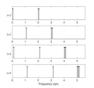
Figure 2: Spectral lines contained in $f_{j}$ for $l$=2, 3, 4, 5

On the other hand, the noise level of accelerometer on board the satellite determines the accuracies of the non-gravitational accelerations, and the error degree power of the non-gravitational acceleration ${\sigma_{\delta{a_{ng}},l}}$, which describes the error average power of the ones introduced by the satellites orbit errors in the $l$-th degree

$${\sigma_{\delta{a_{ng}},l}}=\sqrt{\sum\limits_{j}{\int_{{f_{j}}-\mathrm{\Delta}f}^{{f_{j}}+\mathrm{\Delta}f}{{{\left[{{S_{acc}}(f)}\right]}^{2}}df}}},$$ (40)

where ${S_{acc}}(f)$ is the PSD of the accelerometer measurement noise.

On the basis of Eq. (8), one can derive analytically the direct relationship between the PSD of the LL-SST measurement errors and the coefficients of the Earth’s gravity potential by using the equations derived above. The direct relationship between the PSD of range-rate errors and the coefficients of the Earth’s gravity potential can be derived analytically from Eqs. (27) and (28):

$$\begin{array}[]{*{20}{l}}{{\sigma_{l}}=A\left(l\right){\sigma_{T_{AB}^{\left(x\right)},l}}}\\ \begin{array}[]{l}\;\;\;\;=A\left(l\right)\left\{{\sum\limits_{j}{\left[{\displaystyle\int_{{f_{j}}-\mathrm{\Delta}f/2}^{{f_{j}}+\Delta f/2}{{{\left({{S_{\mathrm{\delta}\dot{\rho}}}(f){H_{\delta\dot{\rho}\to{a_{x}}}}(f)}\right)}^{2}}}df+}\right.}}\right.\\ \;\;\;\;\;\;\;{\left.{\left.{\displaystyle\int_{{f_{j}}-\mathrm{\Delta}f}^{{f_{j}}+\mathrm{\Delta}f}{{{\left({{S_{acc}}(f)}\right)}^{2}}df}}\right]}\right\}^{\frac{1}{2}}}\end{array}\end{array}$$ (45)

for the $x$ directions, and

$$\begin{array}[]{*{20}{l}}{{\sigma_{l}}=B\left(l\right){\sigma_{T_{AB}^{\left(z\right)},l}}}\\ \begin{array}[]{l}\;\;\;\;=B\left(l\right)\left\{{\sum\limits_{j}{\left[{\displaystyle\int_{{f_{j}}-\mathrm{\Delta}f/2}^{{f_{j}}+\Delta f/2}{{{\left({{S_{\mathrm{\delta}\dot{\rho}}}(f){H_{\delta\dot{\rho}\to{a_{z}}}}(f)}\right)}^{2}}}df+}\right.}}\right.\\ \;\;\;\;\;\;\;{\left.{\left.{\displaystyle\int_{{f_{j}}-\mathrm{\Delta}f}^{{f_{j}}+\mathrm{\Delta}f}{{{\left({{S_{acc}}(f)}\right)}^{2}}df}}\right]}\right\}^{\frac{1}{2}}}\end{array}\end{array}$$ (50)

for the $z$ directions. In order to obtain the optimal solution, it is usual to recover the gravity field from the combination of observations in the two directions, which is applied to the following simulations.

4 Relationship between perturbing forces and range-rate perturbations

Using the orbit perturbation theory, this section describes the transfer functions from range-rate perturbations to perturbing accelerations. Based on the assumption of the polar circular orbit, the linearized Hill s equations are adopted here (Colombo 1986; Schrama 1989)

$$\left\{{\begin{array}[]{*{20}{c}}{\ddot{x}+2\omega\dot{z}=\delta{a_{x}}}\\ {\ddot{y}+{\omega^{2}}y=\delta{a_{y}}}\\ {\ddot{z}-2\omega\dot{x}-3{\omega^{2}}z=\delta{a_{z}}}\end{array}}\right.,$$ (54)

where $\omega$ is the mean orbit rate $\omega=\sqrt{GM/{r^{3}}}$, $\delta a_{x}$, $\delta a_{y}$ and $\delta a_{z}$ are the perturbing accelerations in the along-track, cross-track and radial directions, respectively. By applying the state space representation from control system theory, the relationship between the perturbed state and the perturbing accelerations can be expressed in the following state space form (Kim 2000):

$$\left\{{\begin{array}[]{*{20}{c}}{{\bf{\dot{u}}}={\bf{Au}}+{\bf{Ba}}}\\ {{\bf{v}}={\bf{Cu}}}\end{array}}\right.,$$ (57)

where the perturbed state vector of two satellites is

$${\bf{u}}={\left[{{x_{1}},{y_{1}},{z_{1}},{{\dot{x}}_{1}},{{\dot{y}}_{1}},{{\dot{z}}_{1}},{x_{2}},{y_{2}},{z_{2}},{{\dot{x}}_{2}},{{\dot{y}}_{2}},{{\dot{z}}_{2}}}\right]^{T}},$$

the perturbing acceleration vector

$${\bf{a}}={\left[{{a_{{x_{1}}}},{a_{{y_{1}}}},{a_{{z_{1}}}},{a_{{x_{2}}}},{a_{{y_{2}}}},{a_{{z_{2}}}}}\right]^{T}},$$

and the perturbation vector of range-rate due to the perturbing forces

$${\bf{v}}={\left[{\delta\rho,\delta\dot{\rho}}\right]^{T}}.$$

Accordingly, $\bf{A}$ and $\bf{B}$ are the coefficient matrices. Based on the Fig. 1, the intersatellite range-rate satisfy the following equations (Visser 2005):

$$\delta\dot{\rho}=({\dot{z}_{2}}+{\dot{z}_{1}})\sin\frac{\eta}{2}+({\dot{x}_{2}}-{\dot{x}_{1}})\cos\frac{\eta}{2}.$$ (58)

Then $\bf{C}$ can be built in the following way:

$${\bf{C}}=\left[{\begin{array}[]{*{20}{c}}0&0&0&{-\cos\frac{\eta}{2}}&0&{\sin\frac{\eta}{2}}&0&0&0&{\cos\frac{\eta}{2}}&0&{\sin\frac{\eta}{2}}\end{array}}\right].$$

The transfer function ${\bf{G}}(s)$, which maps the PSD of perturbing accelerations into that of range-rate perturbations with zero initial conditions, can be computed analytically in the complex frequency domain (Ogata 2010)

$$\begin{array}[]{l}{\bf{G}}(s)={\bf{C}}{(s{\bf{I}}-{\bf{A}})^{-1}}{\bf{B}}\\ =\left[{\begin{array}[]{*{20}{c}}{{G_{{a_{{x_{1}}}}}}\!\!(s)}&{{G_{{a_{{y_{1}}}}}}\!\!(s)}&{{G_{{a_{{z_{1}}}}}}\!\!(s)}&{{G_{{a_{{x_{2}}}}}}\!\!(s)}&{{G_{{a_{{y_{2}}}}}}\!\!(s)}&{{G_{{a_{{z_{2}}}}}}\!\!(s)}\end{array}}\right].\end{array}$$ (62)

In order to obtain the frequency transfer function ${\bf{G}}(f)$, the complex frequency $s$ is replaced by the frequency $f$ (where $s=2\pi f$). The transfer function ${\bf{H}}(f)$ from the range-rate perturbations into perturbing accelerations is the reciprocal of ${\bf{G}}(f)$ based on their definitions (Cai et al. 2015):

$$\begin{array}[]{l}{\bf{H}}(f)\\ \!\!\!=\!\!\!\left[{\begin{array}[]{*{20}{c}}{{\!\!H_{{a_{{x_{1}}}}}}\!(f)}&{{\!H_{{a_{{y_{1}}}}}}\!(f)}&{{\!H_{{a_{{z_{1}}}}}}\!(f)}&{{\!H_{{a_{{x_{2}}}}}}\!(f)}&{{\!H_{{a_{{y_{2}}}}}}\!(f)}&{{\!H_{{a_{{z_{2}}}}}}\!(f)}\end{array}}\right]\\[5.69054pt] \!\!\!=\!\!\!\left[{\begin{array}[]{*{20}{c}}{\displaystyle\frac{1}{{{\!\!G_{{a_{{x_{1}}}}}}\!(f)}}}&{\displaystyle\!\frac{1}{{{\!G_{{a_{{y_{1}}}}}}\!(f)}}}&{\displaystyle\!\frac{1}{{{\!G_{{a_{{z_{1}}}}}}\!(f)}}}&{\displaystyle\!\frac{1}{{{\!G_{{a_{{x_{2}}}}}}\!(f)}}}&{\displaystyle\!\frac{1}{{{\!G_{{a_{{y_{2}}}}}}\!(f)}}}&{\displaystyle\!\frac{1}{{{\!G_{{a_{{z_{2}}}}}}\!(f)}}}\end{array}}\right].\end{array}$$ (68)

Under the assumption of an orbit height of 450 km, the frequency response of transfers function from the range-rate perturbations to perturbing forces can be obtained from the above results, as shown in Fig. 3.

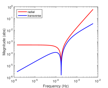
Figure 3: Transfer functions from range-rate perturbations to perturbing forces

5 Simulation and discussion

The method enables us to gain a deeper insight into the error analysis of LL-SST and is useful for mission design and error analysis. Considering the requirements of GRACE-FO, we concentrate on the effects of instrument noises and orbit parameters on the accuracy of the gravity field recovery.

5.1 Sensor noise effects and matching

5.1.1 Noise realizations

The realistic noises of onboard instruments, such as the intersatellite ranging instrument and accelerometer, are generally colored. Based on a synthesis of the requirements from Sheard et al. (2012) and Elsaka et al. (2014), it is assumed that the PSD of a laser interferometer ${S_{\dot{\rho}\_{\rm{LRI}}}}(f)$ is defined by means of the following analytical functions:

$${S_{\dot{\rho}\_{\rm{LRI}}}}(f)\!\!=\!\!2\pi f\sqrt{{{\left({{S_{0}}}\right)}^{2}}\!\!+\!\!\frac{{80}}{f}{{\left({355\!\!\times\!\!{{10}^{-12}}\cdot\frac{\rho}{{100\;{\rm{km}}}}}\right)}^{2}}}$$ (69)

where ${\left({{S_{0}}}\right)^{2}}$ and $80/f{\left({355\times{{10}^{-12}}\cdot\rho/100\;{\rm{km}}}\right)^{2}}$ are the white noise component and frequency-dependent noise component, respectively. $S_{0}$ is generally assigned a value of 50 $\text{nm}/\sqrt{\textrm{Hz}}$ for LRI (Elsaka et al. 2014). The factor $2\pi f$ relates to the conversion of ranges to range-rates.

The main error sources of KBR onboard GRACE-FO are the oscillator and system noise. The PSD of KBR noise model can be written as (Kim 2000)

$${S_{\dot{\rho}\_{\rm{KBR}}}}(f)=2\pi f\sqrt{{{\left[{{S_{{\rm{osc}}}}(f)}\right]}^{2}}+{{\left[{{S_{{\rm{sys}}}}(f)}\right]}^{2}}},$$ (70)

where ${S_{{\rm{osc}}}}(f)$ and ${S_{{\rm{sys}}}}(f)$ are the PSD of the oscillator noise and system noise, respectively. Kim (2000) describes the KBR measurement error due to the oscillator and system noise following the GRACE case. The accelerometer noise model ACC 1 is derived from the sensitive axes of a SuperSTAR-type sensor (Touboul et al. 1999), which is the accelerometer of GRACE (and expectedly also of GRACE-FO). The accelerometer noise contributes are the detector, action, measure, parasitic and thermal noise (Christophe et al. 2010).

In order to discuss the match between accelerometer and range-rate noise in spectral domain, other three accelerometer noise models are introduced in this study, as shown in Table 1.

Table 1: Four accelerometer noise models with different PSD

Model	PSD (unit: ${\rm{m/}}{{\rm{s}}^{2}}/\sqrt{\textrm{Hz}})$	Study (Ref.)
ACC 1	$1\!\!\times\!\!{10^{-10}}\sqrt{1\!\!+\!\!0.005/f}$	GRACE & GRACE–FO (Kim 2000)
ACC 2	$5\!\!\times\!\!{10^{-11}}\sqrt{1\!\!+\!\!0.005/f}$	e2.motion (Gruber et al. 2014)
ACC 3	$1.5\!\!\times\!\!{10^{-12}}\sqrt{1\!\!+\!\!0.005/f}$	NG2 (Anselmi et al. 2011)
ACC 4	$1.5\!\!\times\!\!{10^{-12}}$	—

For comparison’s sake, the analytic transfer function ${\bf{H}}(f)$ is applied in order to convert range-rate perturbations into equivalent the accelerometer noise, and then the accelerometer error is comparable to the range-rate errors. Figure 4 shows the PSD of the accelerometer error due to KBR, LRI and different accelerometer noise models. The total noise is dominated by the ACC noise at the low frequencies (with regard to GRACE-FO, $f<0.8$ mHz for KBR, $f<6$ mHz for LRI), whereas by ranging system noise at the high frequencies. Therefore, it is evident that the accuracy of the low degree gravity coefficients will be mainly affected by the accelerometer noise, whereas the high degree ones be mainly affected by the range system noise.

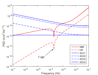
Figure 4: Comparison of the power spectra density of acceleration noises due to range-rate errors and different accelerometer noise models. The red and the dashed red lines denote the KBR noise and the LRI noise, respectively. The blue lines from top to bottom are accelerometer noises ACC 1, ACC 2, ACC 3 and ACC 4, respectively.

5.1.2 Sensor noise effects

The fundamental measurement quantity to be observed in a satellite to satellite tracking mission are the distance variation between the two satellites and the non-gravitational acceleration. This subsection, referring to GRACE-FO, discusses the differences in the recovery caused from KBR and LRI measurement errors with the accelerometer noise ACC 1. For this purpose, the following orbit parameters have been used for the simulation: orbit height 450 km; mission duration 12 months; separation distance 220 km. The PSD of instrument noise, i.e. LRI, KBR and ACC 1, are above mentioned in the last subsection. According to the results obtained in Sect. 3, the error degree amplitudes can be derived from the result of Sect. 3, as shown in Fig. 5. Based on Kaula’s rule, it can be concluded that the maximum recovery degrees of the gravity field models are 197 and 160 for the LRI plus ACC1 and KBR plus ACC1, corresponding to a half wavelength resolution of about 101 and 125 km, respectively. It is obvious from Fig. 5 that the accuracy of the gravity field recovery recovery from LRI plus ACC1 is improved about an order of magnitude better than that from KBR plus ACC1 in the higher degrees ($l>10$). But in the lower degrees ($l<10$) the accuracy can not be improved because accelerometer noise is dominant in this range. The corresponding cumulative geoid height errors are shown in Fig. 6. From Fig. 6 and Table 2, it is seen that the two scenario provide geoids with accuracies of $1.2\times 10^{-2}$ and 4.3 cm at degree 150, and 7.4 and 10.2 cm at their maximum recovery degrees. The model derived from scenario LRI plus ACC 1 is about 35 times better than that from KBR plus ACC 1 measurements except for the lower degrees. It also can be seen from Eqs. (45) and (50) that an $N$ times better range-rate accuracy yields about an $N$ times better gravity field model when other elements remain the same.

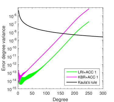
Figure 5: Error degree amplitudes under different scenarios

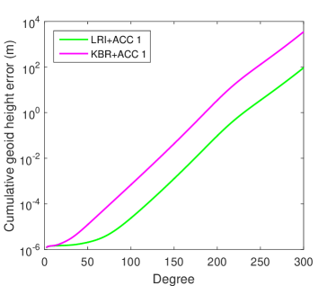
Figure 6: Cumulative geoid height errors under different scenarios

Table 2: Cumulative geoid height errors with different accuracies of range-rates

Sensor noise model	Max. degree	Cumulative geoid height errors (cm)
		@Degree 100	@Degree 150	@Max. degree
LRI+ACC 1	197	$2.4\times 10^{-3}$	$1.2\times 10^{-1}$	7.4
KBR+ACC 1	160	$6.8\times 10^{-2}$	4.3	10.2

5.1.3 Spectral matching of instrument accuracies

The above results show that the accuracies of lower degree coefficients in GRACE-FO are limited by the accelerometer noise, whether inter-satellite range-rate observations provided by KBR or LRI. This subsection discusses the matching relation between range-rate observations and accelerometer noises by taking advantage of the one-to-one correspondence between spherical harmonics and frequencies indicated in the Sect. 3. For this purpose, the following orbit parameters have been used for the simulation: orbit height 450 km; mission duration 30 days; separation distance 220 km. Under these conditions, one can derive the error degree amplitudes of the above-mentioned KBR, LRI and four accelerometer noise models, as shown in Fig. 7. For the sake of clarity, we shall deal with the observations in the $x$ direction, although the observations in the $z$ direction has a similar property.

The comparison of the PSD and error degree amplitudes of sensor noises, i.e. Figs 4 and 7, provides a valuable insight into the spectral matching of instrument accuracies. The PSD of ACC 2 is two times better than that of ACC 1, but accelerometer noise is also dominant compared to KBR error in the lower degrees ($l<8$). This is most obvious at degree 2 which contains the frequencies close to zero frequency and 2 cpr. The error degree amplitudes of ACC 1 are about two orders of magnitude higher than that of KBR error at degree 2. It is critical because the square of ACC 2 PSD is approximation of $1/f$ behavior below 5 mHz. For this reason, the PSD of ACC 2 is about four orders of magnitude higher than that of KBR error at the frequencies close to zero frequency but a mere two times higher at the frequencies close to 2 cpr. Meanwhile, the other even degrees also have this effect due to the fact that they contains the spectral lines close to zero cpr too. Certainly, the effect at lower degrees caused by the $1/f$ behavior is more obvious than higher degrees since the number of high frequencies increases with degrees. A solution to this problem depends on the sufficient suppression of the $1/f$ noise of accelerometers.

In contrast, the error degree amplitudes at odd degrees are unaffected by the frequencies close to zero frequency since they only contain the frequencies close to odd cpr. A significant phenomenon is that error degree amplitudes of the models that contain a pink noise, e.g. ACC 1, ACC 2 and ACC 3, are obviously a saw-tooth curve which fluctuates up and down depending on parity of $l$, crests for $l$ even and troughs for $l$ odd. On the other hand, thanks to the frequency trap of KBR at 1 cpr caused by ${\bf{H}}(f)$, the error degree amplitudes of that at odd degrees are hardly affected by the noise around this frequency. This is the reason why the error degree amplitudes of KBR are lower than that of ACC 2 at degree 3 even if the PSD of them are equal at 3 cpr. When applying ACC 3, which targets a factor of 33 sensitivity improvement over ACC 2, the error degree amplitudes of KBR and accelerometer noises match each other at degree 2. It means that the accuracies of spherical harmonic coefficients at all degrees are determined by KBR noise in this situation, as shown in Fig. 7. Considering the existing state-of-the-art accelerometer accuracy is at the level of around ${10^{-12}}$ ${\rm{m/}}{{\rm{s}}^{2}}/\sqrt{\textrm{Hz}}$ (Drinkwater et al. 2007), it is necessary to make the accuracies of coefficients at lower degrees match each other by removing or suppressing the $1/f$ noise of accelerometers if LR is applied instead of KBR. Compared with the colored noise ACC 3, the white noise ACC 4 gets better match to LR at lower degrees, as shown in Fig. 7. Based on the benefit of the elimination of $1/f$ noise, the error degree amplitudes of ACC 4 are lower than that of ACC 3 at all degrees, although this phenomenon decreases with degrees. For the same reason the saw-tooth behaviour of the error degree amplitude curve disappears and then the accuracies of spherical harmonic coefficients become more homogeneous between even and odd degrees. It is worth studying on the improvement of the accuracy of accelerometers for the match between the range errors and accelerometer noises in the future mission.

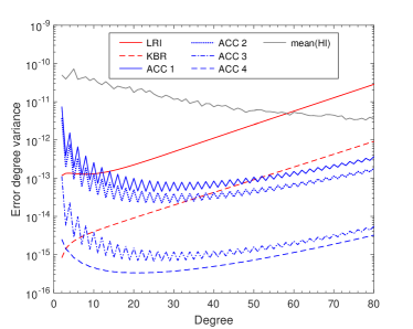
Figure 7: Comparison of error degree amplitudes of different sensor noises. The red and the dashed red lines denote error degree amplitudes derived from the KBR and LRI noise, respectively. The blue lines from top to bottom are error degree amplitudes derived from accelerometer noises ACC 1, ACC 2, ACC 3 and ACC 4, respectively.

5.2 Time variable gravity signal effects

The LL-SST missions can be effectively used for obtaining information on the temporal changes of the Earth s gravity field on a global scale, which has been accompanied by temporal aliasing due to undersampling of unmodeled mass variations (Murböck et al. 2014). The method proposed in this study can also be applied in the analysis of time variable gravity signal effects. To investigate temporal aliasing caused by the time variable gravity signals, the SST-ll observations are computed in terms of range-rate differences along the line-of-sight of two satellites. The parameters of orbit are the same as stated already in the last subsection except for the duration which is 30 days. There are two input time variable gravity signals. The first signal is computed from the the residual AO signal (AO – mean(AO)) from the ESA-AOHIS model (Gruber et al. 2011) and the second signal is computed from the difference of the ocean tide models EOT08a (Savcenko and Bosch 2008) and FES2004 (Lyard et al. 2006).

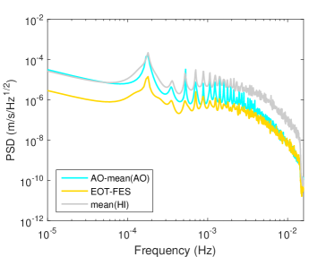
Figure 8: PSD of the difference of the non-tidal oceanic and atmospheric signals and the corresponding mean signal and the difference of the ocean tide models EOT08a and FES2004 together with the mean hydrology plus ice signal. They are computed in terms of range-rate along the line-of-sight of two satellites

Figure 8 shows the PSD of the two signals together with the mean hydrology plus ice signal (mean(HI)) in terms of range-rate differences. It is found that time variable gravity signal effects from the two sources acts on multiples of cpr. As previously mentioned in Sect. 3, the spectral lines contained in $f_{j}$ are close to the multiples of cpr so that the error degree amplitudes derived from the time variable gravity signals are mainly determined by the peaks of their PSD. Figure 9 shows the error degree amplitudes of temporal aliasing from both non-tidal and tidal sources including two types of sensor noise together with the mean hydrology plus ice signal. From fig. 9, it can be seen that error degree amplitudes of the residual AO signals intersect that of mean hydrology plus ice signal at degree 70, corresponding to a half wavelength resolution of about 286 km. The error degree amplitudes of the difference of the ocean tide models EOT08a and FES2004 are about one order of magnitude lower than that of the residual AO signals. If KBR and ACC 1 are adopted as the sensor noises then the maximum recovery degree of hydrology plus ice signal models is 58. In this case, the temporal aliasing mainly determines the model accuracy at the degrees lower than 45, whereas sensor noise mainly determines that at degrees from 45 to 58. If LRI and ACC 1 are adopted as the sensor noises then the model accuracy are almost totally determined by the temporal aliasing. As a result, temporal aliasing due to undersampling of unmodelled high frequency mass variations will be one of the most serious problems for future gravity missions which use high quality sensors (Gruber et al. 2014).

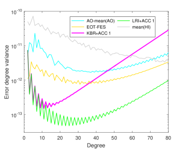
Figure 9: Error degree amplitudes of temporal aliasing from both non-tidal and tidal sources including two types of sensor noise together with the mean hydrology plus ice signal.

6 Conclusion

Based on the spectral analysis and orbit perturbation theory, an analytical relationship between the PSD of LL-SST measurements and the accuracies of gravity field coefficients is presented mainly from the point of view of theory of signal and system, which indicates the one-to-one correspondence between spherical harmonic error degree variances and frequencies of the measurement noise. This relationship provides a physical insight into how the measurement noises affect the accuracy of the gravity field recovery. The method is an efficient and convenient tool for the design of future mission, especially for high accuracy and resolution gravity field models. By taking GRACE-FO as the object of research, the effects of sensor noises and time variable gravity signals are analyzed. If LRI measurements are applied, a mission goal with a geoid accuracy of 7.4 cm at a spatial resolution of 101 km is reachable, whereas if the KBR measurement error model is applied, a mission goal with a geoid accuracy of 10.2 cm at a spatial resolution of 125 km is reachable. The spectral matching of instrument accuracies is also investigated by taking the advantage of the analytical relationship. It is necessary to improve the accuracy of accelerometers for the match between the range errors and accelerometer noises in the future mission, especially for removing or suppressing the 1/f noise. Temporal aliasing caused by the time variable gravity signals is also discussed by this method. The one-to-one correspondence in the spectral domain may provide a way for reducing the aliasing effects, but this still needs further study based on the actual data.

This study is based on the hypothesis that the satellite orbit is a polar circular orbit, while the realistic orbit with an inhomogeneous data distribution should cause a lower accuracy and resolution model. It should be noted that the gravity signal can not exactly recovered according to the Nyquist theorem if polar gaps occurs with a non-polar inclination. In this case the results of error propagation computed by least-square methods are fitted values, unless the gaps are filled with other data. Furthermore, the linear orbit perturbation theory is adopted, which means that we have ignored the higher-order effect terms. Notwithstanding its limits, the essential relationship is clearly indicated. Further improvements in all these problems need to be further analyzed.

Appendix: Average power of the error of gravitational acceleration difference in the $x$ direction

The expression for the average power of gravitational acceleration difference errors is the key element for obtaining the analytical relationship between the PSD of LL-SST measurements and the accuracies of gravity field coefficients. Since the derivatives of the gravitational potential in the $z$ direction keep the orthogonality property of spherical harmonics, it is easy to deduce the power of the errors of gravitational acceleration difference by applying Parseval’s theorem, as shown in Eq. (22). On the contrary, the derivatives of the gravitational potential in the $x$ direction relate to the derivatives with respect to co-latitude and loose the orthogonality property of spherical harmonics, so Parseval’s theorem cannot be applied directly in this situation. In this section, the average power of gravitational acceleration difference errors in the $x$ direction is obtained based on the definition of spherical harmonics and the integration property of associated Legendre functions.

According to Eq. (18), the average power of gravitational acceleration difference error in the $x$ direction can be expanded as

$$\begin{array}[]{l}\sigma_{T_{AB}^{\left(x\right)}}^{2}\!\!=\!\!\displaystyle\frac{1}{{4\pi}}\int_{\sigma}{{{\left({T_{AB}^{\left(x\right)}}\right)}^{2}}d\sigma}\\ \;\;\;\;\;\;\;\;\;\!\!=\!\!\displaystyle\frac{1}{{4\pi}}\!\!\iint_{S}{\left[{{{\left({\frac{{\partial{T_{A}}}}{{\partial x}}}\right)}^{2}}\!\!+\!\!{{\left({\frac{{\partial{T_{B}}}}{{\partial x}}}\right)}^{2}}\!\!-\!\!2\frac{{\partial{T_{A}}}}{{\partial x}}\frac{{\partial{T_{B}}}}{{\partial x}}}\right]}\times\\[11.38109pt] \;\;\;\;\;\;\;\;\;\;\;\sin\theta d\theta d\lambda.\end{array}$$ (74)

Substitution of Eq. (9) into above equation yields

$$\begin{array}[]{*{20}{l}}{\sigma_{T_{AB}^{\left(x\right)}}^{2}\!\!=\!\!\displaystyle\frac{1}{{4\pi}}{{\left({\frac{{GM}}{{rR}}}\right)}^{2}}\!\!\iint_{S}\!\!{\left\{{\left[{{{\sum\limits_{l=2}^{\infty}{\left({\frac{R}{r}}\right)}}^{2\left({l+1}\right)}}\!\!\sum\limits_{m=0}^{l}\!\!{\left({{{\bar{C}}_{lm}}}\right.\times}}\right.}\right.}}\\ {\;\;\;\;\;\;\;\;\;{{\left.{\left.{\cos m{\lambda_{A}}+{{\bar{S}}_{lm}}\sin m{\lambda_{A}}}\right)\displaystyle\frac{{d{{\bar{P}}_{lm}}(\cos{\theta_{A}})}}{{d\theta}}}\right]}^{2}}\times}\\ \begin{array}[]{l}\;\;\;\;\;\;\;\;\;\sin\theta d\theta d\lambda+\left[{{{\sum\limits_{l=2}^{\infty}{\left({\displaystyle\frac{R}{r}}\right)}}^{2\left({l+1}\right)}}\sum\limits_{m=0}^{l}{\left({{{\bar{C}}_{lm}}}\right.\times}}\right.\\ \;\;\;\;\;\;\;\;\;{\left.{\left.{\cos m{\lambda_{B}}+{{\bar{S}}_{lm}}\sin m{\lambda_{B}}}\right)\displaystyle\frac{{d{{\bar{P}}_{lm}}(\cos{\theta_{B}})}}{{d\theta}}}\right]^{2}}\times\\ \;\;\;\;\;\;\;\;\;\sin\theta d\theta d\lambda-2\sum\limits_{l=2}^{\infty}{{{\left({\displaystyle\frac{R}{r}}\right)}^{2\left({l+1}\right)}}\sum\limits_{m=0}^{l}{\left[{\left({{{\bar{C}}_{lm}}\times}\right.}\right.}}\\ \;\;\;\;\;\;\;\;\;\left.{\left.{\cos m{\lambda_{A}}+{{\bar{S}}_{lm}}\sin m{\lambda_{A}}}\right)\displaystyle\frac{{d{{\bar{P}}_{lm}}(\cos{\theta_{A}})}}{{d\theta}}}\right]\times\end{array}\\ \begin{array}[]{l}\;\;\;\;\;\;\;\;\;\sum\limits_{l=2}^{\infty}{{{\left({\displaystyle\frac{R}{r}}\right)}^{2\left({l+1}\right)}}\sum\limits_{m=0}^{l}{\left[{\left({{{\bar{C}}_{lm}}\cos m{\lambda_{B}}+{{\bar{S}}_{lm}}\times}\right.}\right.}}\\ \;\;\;\;\;\;\;\;\;\left.{\left.{\sin m{\lambda_{B}}}\right)\displaystyle\frac{{d{{\bar{P}}_{lm}}(\cos{\theta_{B}})}}{{d\theta}}}\right]\times\;\sin\theta d\theta d\lambda\Bigg{\}}.\end{array}\\ \end{array}$$ (85)

For a specific value of $l$, the summation over $l$ at the right-hand side of Eq. (85) should be removed, and the error average power $\sigma_{T_{AB}^{\left(x\right)}}^{2}$ at the left-hand side replaced with the error degree power $\sigma_{T_{AB}^{\left(x\right)},l}^{2}$ , can be obtained as follows:

$$\begin{array}[]{*{20}{l}}\begin{array}[]{l}\sigma_{T_{AB}^{\left(x\right)},l}^{2}={\left({\displaystyle\frac{{GM}}{{rR}}}\right)^{2}}{\left({\displaystyle\frac{R}{r}}\right)^{2\left({l+1}\right)}}\left\{{\displaystyle\frac{1}{{4\pi}}\iint\limits_{S}{\left[{\sum\limits_{m=0}^{l}{\left({{{\bar{C}}_{lm}}\times}\right.}}\right.}}\right.\\ \;\;\;\;\;\;\;\;\;\;\;\;{\left.{\left.{\cos m{\lambda_{A}}+{{\bar{S}}_{lm}}\sin m{\lambda_{A}}}\right)\displaystyle\frac{{d{{\bar{P}}_{lm}}(\cos{\theta_{A}})}}{{d\theta}}}\right]^{2}}\times\\ \;\;\;\;\;\;\;\;\;\;\;\;\sin\theta d\theta d\lambda+\displaystyle\frac{1}{{4\pi}}\iint\limits_{S}{\left[{\sum\limits_{m=0}^{l}{\left({{{\bar{C}}_{lm}}\cos m{\lambda_{B}}+}\right.}}\right.}\\ \;\;\;\;\;\;\;\;\;\;\;\;{\left.{\left.{{{\bar{S}}_{lm}}\sin m{\lambda_{B}}}\right)\displaystyle\frac{{d{{\bar{P}}_{lm}}(\cos{\theta_{B}})}}{{d\theta}}}\right]^{2}}\sin\theta d\theta d\lambda-\end{array}\\ {\;\;\;\;\;\;\;\;\;\;\;\;\displaystyle\frac{2}{{4\pi}}\iint\limits_{S}{\sum\limits_{m=0}^{l}{\bigg{[}\left({{{\bar{C}}_{lm}}\cos m{\lambda_{A}}+{{\bar{S}}_{lm}}\sin m{\lambda_{A}}}\right)\times}}}\\ {\;\;\;\;\;\;\;\;\;\;\;\;\displaystyle\frac{{d{{\bar{P}}_{lm}}(\cos{\theta_{A}})}}{{d\theta}}\cdot\sum\limits_{m=0}^{l}{\left({{{\bar{C}}_{lm}}\cos m{\lambda_{B}}+{{\bar{S}}_{lm}}\times}\right.}}\\ {\;\;\;\;\;\;\;\;\;\;\;\;\left.{\left.{\sin m{\lambda_{B}}}\right)\displaystyle\frac{{d{{\bar{P}}_{lm}}(\cos{\theta_{B}})}}{{d\theta}}}\right]\sin\theta d\theta d\lambda\Bigg{\}}.}\end{array}$$ (94)

Owing to the orthogonality of trigonometric functions, the summations over $l$ can be moved outside of the square brackets, then one obtains

$$\begin{array}[]{*{20}{l}}\begin{array}[]{l}\sigma_{T_{AB}^{\left(x\right)},l}^{2}={\left({\displaystyle\frac{{GM}}{{rR}}}\right)^{2}}{\left({\displaystyle\frac{R}{r}}\right)^{2\left({l+1}\right)}}\left\{{\displaystyle\frac{1}{{4\pi}}\sum\limits_{m=0}^{l}{\displaystyle\iint\limits_{S}{\bigg{[}\left({{{\bar{C}}_{lm}}\times}\right.}}}\right.\\ {\left.{\left.{\;\;\;\;\;\;\;\;\cos m{\lambda_{A}}+{{\bar{S}}_{lm}}\sin m{\lambda_{A}}}\right)\displaystyle\frac{{d{{\bar{P}}_{lm}}(\cos{\theta_{A}})}}{{d\theta}}}\right]^{2}}\times\end{array}\\ \begin{array}[]{l}\;\;\;\;\;\;\;\;\sin\theta d\theta d\lambda+\displaystyle\frac{1}{{4\pi}}\displaystyle\sum\limits_{m=0}^{l}{\iint\limits_{S}{\bigg{[}\left({{{\bar{C}}_{lm}}\cos m{\lambda_{B}}+}\right.}}\\ \;\;\;\;\;\;\;\;{\left.{\left.{{{\bar{S}}_{lm}}\sin m{\lambda_{B}}}\right)\displaystyle\frac{{d{{\bar{P}}_{lm}}(\cos{\theta_{B}})}}{{d\theta}}}\right]^{2}}\sin\theta d\theta d\lambda-\end{array}\\ {\;\;\;\;\;\;\;\;\displaystyle\frac{2}{{4\pi}}\sum\limits_{m=0}^{l}{\iint\limits_{S}{\bigg{[}\left({{{\bar{C}}_{lm}}\cos m{\lambda_{A}}+{{\bar{S}}_{lm}}\sin m{\lambda_{A}}}\right)\times}}}\\ {\;\;\;\;\;\;\;\;\displaystyle\frac{{d{{\bar{P}}_{lm}}(\cos{\theta_{A}})}}{{d\theta}}\left({{{\bar{C}}_{lm}}\cos m{\lambda_{B}}+{{\bar{S}}_{lm}}\times}\right.}\\ {\;\;\;\;\;\;\;\;\left.{\left.{\sin m{\lambda_{B}}}\right)\displaystyle\frac{{d{{\bar{P}}_{lm}}(\cos{\theta_{B}})}}{{d\theta}}}\right]\sin\theta d\theta d\lambda\}}.\end{array}$$ (104)

The part between the brace in Eq. (104) consists of three integrals:

the first integral I1

$$\begin{array}[]{l}{\rm{I}}1=\displaystyle\frac{1}{{4\pi}}\sum\limits_{m=0}^{l}{\iint_{S}{\left.\bigg{[}{\left({{{\bar{C}}_{lm}}\cos m{\lambda_{A}}+{{\bar{S}}_{lm}}\sin m{\lambda_{A}}}\right)\times}\right.}}\\ \;\;\;\;\;\;{\left.{\displaystyle\frac{{d{{\bar{P}}_{lm}}(\cos{\theta_{A}})}}{{d\theta}}}\right]^{2}}\sin\theta d\theta d\lambda,\end{array}$$ (107)

the second integral I2

$$\begin{array}[]{l}{\rm{I}}2=\displaystyle\frac{1}{{4\pi}}\sum\limits_{m=0}^{l}{\iint_{S}{\left.\bigg{[}{\left({{{\bar{C}}_{lm}}\cos m{\lambda_{B}}+{{\bar{S}}_{lm}}\sin m{\lambda_{B}}}\right)\times}\right.}}\\ \;\;\;\;\;\;{\left.{\displaystyle\frac{{d{{\bar{P}}_{lm}}(\cos{\theta_{B}})}}{{d\theta}}}\right]^{2}}\sin\theta d\theta d\lambda,\end{array}$$ (110)

and the third integral I3

$$\begin{array}[]{*{20}{l}}\begin{array}[]{l}{\rm{I}}3=\displaystyle\frac{1}{{4\pi}}\sum\limits_{m=0}^{l}{\iint\limits_{S}{\left.\bigg{[}{\left({{{\bar{C}}_{lm}}\cos m{\lambda_{A}}+{{\bar{S}}_{lm}}\sin m{\lambda_{A}}}\right)\times}\right.}}\\ \;\;\;\;\left({{{\bar{C}}_{lm}}\cos m{\lambda_{B}}+{{\bar{S}}_{lm}}\sin m{\lambda_{B}}}\right)\displaystyle\frac{{d{{\bar{P}}_{lm}}(\cos{\theta_{A}})}}{{d\theta}}\times\end{array}\\ {\left.{\;\;\;\;\displaystyle\frac{{d{{\bar{P}}_{lm}}(\cos{\theta_{B}})}}{{d\theta}}}\right]\sin\theta d\theta d\lambda}.\end{array}$$ (115)

We only need to deal with two integrals since the first and second integrals are the same in nature.

1.1 Computation of the first and second integrals I1 & I2

In order to obtain of the first and second integral, we first compute it for a specific value of $m$:

$$\begin{array}[]{l}{\rm{I}}{1_{m}}=\displaystyle\frac{1}{{4\pi}}\iint_{S}{\left[{\left({{{\bar{C}}_{lm}}\cos m\lambda+{{\bar{S}}_{lm}}\sin m\lambda}\right)}\right.}\\ \;\;\;\;\;\;\;{\left.{\displaystyle\frac{{d{{\bar{P}}_{lm}}(\cos\theta)}}{{d\theta}}}\right]^{2}}\sin\theta d\theta d\lambda,\end{array}$$ (118)

Considering the relationship between fully normalized Legendre polynomials and unnormalized ones

$${\bar{P}_{lm}}(\cos\theta)=\sqrt{k(2l+1)\frac{{(l-m)!}}{{(l+m)!}}}{P_{lm}}(\cos\theta),$$ (119)

where

$$k=\left\{{\begin{array}[]{*{20}{c}}{1\;\;\;{\rm{for}}\;m=0}\\ {2\;\;\;{\rm{for}}\;m\neq 0}\end{array}}\right.,$$

${\rm{I}}{1_{m}}$ becomes

$$\begin{array}[]{l}{\rm{I}}{1_{m}}=\displaystyle\frac{1}{{4\pi}}{\left({\sqrt{k(2l+1)\frac{{(l-m)!}}{{(l+m)!}}}}\right)^{2}}\times\\ \;\;\;\;\;\;\;\;\displaystyle\int\limits_{0}^{\pi}{{{\left({\displaystyle\frac{{d{P_{lm}}(\cos\theta)}}{{d\theta}}}\right)}^{2}}\sin\theta d\theta\displaystyle\int\limits_{0}^{2\pi}{\left({\bar{C}_{lm}^{2}\times}\right.}}\\ \;\;\;\;\;\;\;\;\left.{{{\cos}^{2}}m\lambda+\bar{S}_{lm}^{2}{{\sin}^{2}}m\lambda}\right)d\lambda.\end{array}$$ (123)

Substituting

$$\int_{0}^{2\pi}{{{\sin}^{2}}m\lambda d\lambda}=\left\{{\begin{array}[]{*{20}{c}}{0\;(m=0)}\\ {\pi\;(m\neq 0)}\end{array}}\right.$$ (126)

and

$$\int_{0}^{2\pi}{{{\cos}^{2}}m\lambda d\lambda}=\left\{{\begin{array}[]{*{20}{c}}{\pi\;\;\;(m\neq 0)}\\ {2\pi\;(m=0)}\end{array}}\right.$$ (129)

into Eq. (123) yields

$$\begin{array}[]{l}{\rm{I}}{1_{m}}=\displaystyle\frac{1}{2}(2l\!+\!1)\displaystyle\frac{{(l\!-\!m)!}}{{(l\!+\!m)!}}\sigma_{lm}^{2}\int_{0}^{2\pi}\!\!{{{\left({\displaystyle\frac{{d{P_{lm}}(\cos\theta)}}{{d\theta}}}\right)}^{2}}\times}\\ \;\;\;\;\;\;\;\;\;\;\;\sin\theta d\theta,\end{array}$$ (132)

where

$$\sigma_{lm}^{2}=\left({\sigma_{{{\bar{C}}_{lm}}}^{2}+\sigma_{{{\bar{S}}_{lm}}}^{2}}\right).$$

is the error degree-order variance. Since the first derivative of Legendre polynomials has a recurrence property in the following form

$$\begin{array}[]{l}\displaystyle\frac{{d{P_{lm}}(\cos\theta)}}{{d\theta}}=\frac{1}{2}\left[{(l+m)(l-m+1)\times}\right.\\ \;\;\;\;\;\;\;\;\;\;\;\;\;\;\;\;\;\;\;\;\;\;\;\left.{P_{l(m-1)}(\cos\theta)-P_{l(m+1)}(\cos\theta)}\right].\end{array}$$ (135)

Eq. (132) becomes

$$\begin{array}[]{*{20}{l}}\begin{array}[]{l}{\rm{I}}{1_{m}}=\left({\displaystyle\frac{{\left({2l+1}\right)}}{2}\displaystyle\frac{{\left({l-m}\right)!}}{{\left({l+m}\right)!}}}\right)\sigma_{lm}^{2}\displaystyle\int\limits_{0}^{\pi}{\displaystyle\frac{1}{4}\left\{{\left[{{{\left({l+m}\right)}^{2}}\times}\right.}\right.}\\ \;\;\;\;\;\;\;{\left.{{{\left({l-m+1}\right)}^{2}}P_{l(m-1)}\left({\cos\theta}\right)}\right]^{2}}-2\left({l+m}\right)\times\end{array}\\ {\;\;\;\;\;\;\;\;\left({l-m+1}\right)P_{l(m-1)}\left({\cos\theta}\right)P_{l(m+1)}\left({\cos\theta}\right)+}\\ {\;\;\;\;\;\;\;\;{{\left[{P_{l(m+1)}\left({\cos\theta}\right)}\right]}^{2}}\bigg{\}}\sin\theta d\theta.}\end{array}$$ (141)

Letting $x=\cos\theta$, then

$$\begin{array}[]{*{20}{l}}\begin{array}[]{l}{\rm{I}}{1_{m}}=-\displaystyle\frac{1}{4}\left({\displaystyle\frac{{\left({2l+1}\right)}}{2}\displaystyle\frac{{\left({l-m}\right)!}}{{\left({l+m}\right)!}}}\right)\sigma_{lm}^{2}\displaystyle\int\limits_{-1}^{1}{\left\{{\left[{{{\left({l+m}\right)}^{2}}\times}\right.}\right.}\\ \;\;\;\;\;\;\;{\left.{{{\left({l-m+1}\right)}^{2}}P_{l(m-1)}\left(x\right)}\right]^{2}}-2\left({l+m}\right)\times\\ \;\;\;\;\;\;\;\left({l-m+1}\right)P_{l(m-1)}\left(x\right)P_{l(m+1)}\left(x\right)+\end{array}\\ {\left.{\;\;\;\;\;\;\;{{\left[{P_{l(m+1)}\left(x\right)}\right]}^{2}}}\right\}{\rm{d}}x.}\end{array}$$ (147)

Eq. (147) has three basic integrals:

$$\textrm{(A)}\;\;\int_{-1}^{1}{{{\left[{P_{l(m-1)}\left(x\right)}\right]}^{2}}dx},$$

$$\textrm{(B)}\;\;\int_{-1}^{1}{{{\left[{P_{l(m+1)}\left(x\right)}\right]}^{2}}dx},$$

$$\textrm{(C)}\;\;\int_{-1}^{1}{P_{l(m+1)}\left(x\right)P_{l(m-1)}\left(x\right)dx}.$$

Based on the formula for computing the modulus of associated Legendre functions, one can obtain the results of integrals A and B as follows:

$$\int_{-1}^{1}{{{\left({P_{l(m-1)}\left(x\right)}\right)}^{2}}dx}=\frac{2}{{2l+1}}\frac{{(l+m-1)!}}{{\left({l-m+1}\right)!}},$$ (148)

$$\int_{-1}^{1}{{{\left({P_{l(m+1)}\left(x\right)}\right)}^{2}}dx}=\frac{2}{{2l+1}}\frac{{(l+m+1)!}}{{\left({l-m-1}\right)!}}.$$ (149)

We resolve integral C with the definition of associated Legendre function. Substitution the Rodrigues’ formula

$$P_{lm}(x)=\frac{{{{(1-{x^{2}})}^{\frac{m}{2}}}}}{{{2^{l}}l!}}\frac{{{d^{l+m}}}}{{d{x^{l+m}}}}{\left({{x^{2}}-1}\right)^{l}}$$ (150)

into integral C yields

$$\begin{array}[]{l}\begin{array}[]{*{20}{l}}{\displaystyle\int\limits_{-1}^{1}{{P_{l(m+1)}}(x){P_{l(m-1)}}(x)dx}}\\ {\;=\displaystyle\frac{1}{{{2^{2l}}l!l!}}\displaystyle\int\limits_{-1}^{1}{{{\left({1-{x^{2}}}\right)}^{\frac{{m-1}}{2}+\frac{{m+1}}{2}}}\displaystyle\frac{{{d^{l+m-1}}}}{{{d^{l+m-1}}}}{{\left({{x^{2}}-1}\right)}^{l}}\times}}\end{array}\\ \;\;\;\;\displaystyle\frac{{{d^{l+m+1}}}}{{{d^{l+m+1}}}}{\left({{x^{2}}-1}\right)^{l}}dx.\end{array}$$ (155)

Letting $X={x^{2}}-1$, then

$$\begin{array}[]{l}\displaystyle\int_{-1}^{1}{{P_{l(m+1)}}(x){P_{l(m-1)}}(x)dx}\\ \;{\rm{=}}\displaystyle\frac{{{{\left({-1}\right)}^{m}}}}{{{2^{2l}}l!l!}}\displaystyle\int_{-1}^{1}{{X^{m}}\displaystyle\frac{{{d^{l+m-1}}{X^{l}}}}{{d{x^{l+m-1}}}}\displaystyle\frac{{{d^{l+m+1}}{X^{l}}}}{{d{x^{l+m+1}}}}}dx.\end{array}$$ (158)

Before doing the integration, it is noted that all derivatives of the function ${X^{m}}$ up to the $(m-1)$-th derivative have (${x^{2}}-1$) as a factor, and are therefore zero at $x=\pm 1$ . If we integrate Eq. (158) by parts we get

$$\begin{array}[]{l}\displaystyle\int\limits_{-1}^{1}{{P_{l(m+1)}}(x){P_{l(m-1)}}(x)dx}\\ \;\;\;\;{\rm{=}}\displaystyle\frac{{{{\left({-1}\right)}^{m}}}}{{{2^{2l}}l!l!}}\displaystyle\int\limits_{-1}^{1}{{X^{m}}\displaystyle\frac{{{d^{l+m+1}}{X^{l}}}}{{d{x^{l+m+1}}}}\displaystyle\frac{{{d^{l+m-1}}{X^{l}}}}{{d{x^{l+m-1}}}}}dx\\ \;\;\;\;=\displaystyle\frac{{{{\left({-1}\right)}^{m}}}}{{{2^{2l}}l!l!}}\left[{\left.{{X^{m}}\displaystyle\frac{{{d^{l+m+1}}{X^{l}}}}{{d{x^{l+m+1}}}}\cdot\displaystyle\frac{{{d^{l+m-2}}{X^{l}}}}{{d{x^{l+m-2}}}}}\right|_{-1}^{1}}\right.\times\\ \;\;\;\;\;\;\;\left.{-\displaystyle\int\limits_{-1}^{1}{\displaystyle\frac{{{d^{l+m-2}}{X^{l}}}}{{d{x^{l+m-2}}}}\displaystyle\frac{d}{{dx}}\left({{X^{m}}\frac{{{d^{l+m+1}}{X^{l}}}}{{d{x^{l+m+1}}}}}\right)}dx}\right].\end{array}$$ (163)

Owing to the condition just stated, the boundary term at the start is zero. We can continue by integrating the remaining integral by parts with throwing away the boundary term until we have done $(l+m-1)$ integrations. At this point one can obtain

$$\begin{array}[]{l}\begin{array}[]{*{20}{l}}\begin{array}[]{l}\displaystyle\int\limits_{-1}^{1}{{P_{lm}}(x){P_{l(m-1)}}(x)dx}\\ \;\;=\displaystyle\frac{{{{\left({-1}\right)}^{m}}{{(-1)}^{l+m-1}}}}{{{2^{2l}}l!l!}}\displaystyle\int\limits_{-1}^{1}{X^{l}}\displaystyle\frac{{{d^{l+m-1}}}}{{d{x^{l+m-1}}}}\end{array}\\ {\;\;\;\;\;\left({{X^{m}}\displaystyle\frac{{{d^{l+m+1}}{X^{l}}}}{{d{x^{l+m+1}}}}}\right)dx}.\end{array}\end{array}$$ (169)

Because that the largest power of $x$ in ${X^{l}}$ and ${X^{m}}$ is ${x^{2l}}$ and ${x^{2m}}$, respectively, one can deduce that the item with the largest power of ${X^{m}}\frac{{{d^{l+m+1}}{X^{l}}}}{{d{x^{l+m+1}}}}$ is $\frac{{\left({2l}\right)!}}{{\left({l-m-1}\right)!}}{x^{l+m-1}}$, and

$$\begin{array}[]{l}\displaystyle\frac{{{d^{l+m-1}}}}{{d{x^{l+m-1}}}}\left({{X^{m}}\displaystyle\frac{{{d^{l+m+1}}{X^{l}}}}{{d{x^{l+m+1}}}}}\right)\\[11.38109pt] \;\;=\displaystyle\frac{{\left({2l}\right)!}}{{\left({l-m-1}\right)!}}\left({l+m-1}\right)!.\end{array}$$ (172)

Then Eq. (169) can be written as

$$\begin{array}[]{*{20}{l}}\begin{array}[]{l}\displaystyle\int\limits_{-1}^{1}{P_{l(m+1)}}(x){P_{l(m-1)}}(x)dx\\ \;\;\;=\displaystyle\frac{{{{\left({-1}\right)}^{m}}{{(-1)}^{l+m-1}}}}{{{2^{2l}}l!l!}}\displaystyle\frac{{\left({2l}\right)!}}{{\left({l-m-1}\right)!}}\left({l+m-1}\right)!\times\end{array}\\ {\;\;\;\;\;\;\displaystyle\int\limits_{-1}^{1}{{X^{l}}dx}}.\end{array}$$ (177)

The integral in Eq. (177) can be solved in the following form

$$\int_{-1}^{1}{{X^{l}}dx}=\int_{-1}^{1}{{{\left({{x^{2}}{\rm{-}}1}\right)}^{l}}dx}={\left({-1}\right)^{l}}\frac{{{{\left({l!}\right)}^{2}}{2^{2l+1}}}}{{\left({2l+1}\right)!}},$$ (178)

so plugging this into Eq. (177) we find that

$$\begin{array}[]{*{20}{l}}\begin{array}[]{l}\displaystyle\int\limits_{-1}^{1}{{P_{l(m+1)}}(x){P_{l(m-1)}}(x)dx(x)dx}\\ \;\;=\displaystyle\frac{{{{\left({-1}\right)}^{m}}{{(-1)}^{l+m-1}}}}{{{2^{2l}}l!l!}}\displaystyle\frac{{\left({2l}\right)!}}{{\left({l-m-1}\right)!}}\times\end{array}\\[28.45274pt] {\;\;\;\;\;\;\left({l+m-1}\right)!{{\left({-1}\right)}^{l}}\displaystyle\frac{{{{\left({l!}\right)}^{2}}{2^{2l+1}}}}{{\left({2l+1}\right)!}}}\\[5.69054pt] {\;\;=-\displaystyle\frac{{\left({l+m-1}\right)!}}{{\left({l-m-1}\right)!}}\displaystyle\frac{2}{{\left({2l+1}\right)}}}\end{array}$$ (184)

Substitution of Eqs. (148), (149) and (184) into Eq. (147) yields

$$\begin{array}[]{*{20}{l}}{{\rm{I}}{1_{m}}=\displaystyle\frac{1}{4}\left({\displaystyle\frac{{\left({2l+1}\right)}}{2}\displaystyle\frac{{\left({l-m}\right)!}}{{\left({l+m}\right)!}}}\right)\sigma_{lm}^{2}\left\{{{{\left({l+m}\right)}^{2}}\times}\right.}\\[11.38109pt] {\;\;\;\;\;\;{{\left({l-m+1}\right)}^{2}}\displaystyle\frac{2}{{2l+1}}\displaystyle\frac{{(l+m-1)!}}{{\left({l-m+1}\right)!}}-2\times}\\[11.38109pt] \begin{array}[]{l}\;\;\;\;\;\;\left({l+m}\right)\left({l-m+1}\right)\left[{-\displaystyle\frac{{\left({l+m-1}\right)!}}{{\left({l-m-1}\right)!}}\displaystyle\frac{2}{{\left({2l+1}\right)}}}\right]+\\[11.38109pt] \;\;\;\;\;\;\left.{\displaystyle\frac{2}{{2l+1}}\displaystyle\frac{{(l+m+1)!}}{{\left({l-m-1}\right)!}}}\right\}\end{array}\\[28.45274pt] {\;\;\;\;\;\;=\sigma_{lm}^{2}\left({{l^{2}}+l-lm-\displaystyle\frac{m}{2}}\right)}.\end{array}$$ (191)

Owing to the following relationship

$${\rm{I}}1=\sum\limits_{m}{{\rm{I}}{1_{m}}}$$ (192)

and the fact that there are $(2l+1)$ linearly independent spherical harmonics in the $l$-th degree, which relates to only one spherical harmonic ${P_{l}}\left({\cos\theta}\right)$ for $m=0$, and two spherical harmonics, i.e. ${P_{lm}}(\cos\theta)sin\left({m\lambda}\right)$ and ${P_{lm}}(\cos\theta)\cos\left({m\lambda}\right)$, for $m=1,2,...,l$, one can compute the integral I1 as follows:

$$\begin{array}[]{l}{\rm{I}}1={\left.{\sigma_{lm}^{2}\left({{l^{2}}+l-lm-\displaystyle\frac{m}{2}}\right)}\right|_{m=0}}+\\ \;\;\;\;\;\;\;\;2\sum\limits_{m=1}^{l}{\sigma_{lm}^{2}\left({{l^{2}}+l-lm-\displaystyle\frac{m}{2}}\right)}.\end{array}$$ (195)

We assume that the error powers of these $(2l+1)$ spherical harmonics $\sigma_{lm}^{2}$ are equal. This is reasonable because the temporal spectral lines of spherical harmonics of the same degree are in close proximity and ones of different degrees are farther apart (Cai et al. 2013a). Therefore, the effects of instrument noise on the error powers of spherical harmonics in the same degree are nearly equal, especially for the white noise. Then, Eq. (195) can be computed as

$${\rm{I}}1=\frac{1}{2}l\left({1+l}\right)\left({2l+1}\right)\sigma_{lm}^{2}.$$ (196)

Noticing that (Rummel et al. 1993)

$$\sigma_{l}^{2}=\left({2l+1}\right)\sigma_{lm}^{2},$$ (197)

then

$${\rm{I}}1=\frac{1}{2}l\left({1+l}\right)\sigma_{l}^{2}.$$ (198)

In the same way,

$${\rm{I}}2=\frac{1}{2}l\left({1+l}\right)\sigma_{l}^{2}.$$ (199)

1.2 Computation of the third integral

The integral I3 can be dealt with by applying the properties of the covariance function of spherical function. First, we define a square integrable and analytical function $f(\theta,\lambda)$ which is expanded in a series of spherical harmonics on the unit sphere

$$\begin{array}[]{l}f(\theta,\lambda)=\sum\limits_{l=0}^{\infty}{\sum\limits_{m=0}^{l}{{{\bar{P}}_{lm}}(\cos\theta)\left({{{\bar{C}}_{lm}}\cos m\lambda+}\right.}}\\[11.38109pt] \;\;\;\;\;\;\;\;\;\;\;\;\;\;\left.{{{\bar{S}}_{lm}}\sin m\lambda}\right).\end{array}$$ (202)

The covariance function of $f(\theta,\lambda)$ at points A and B can be presented as follows:

$$\begin{array}[]{*{20}{l}}\begin{array}[]{l}{\rm{Cov}}\left({f(A),f(B)}\right)\\ \;\;=\displaystyle\frac{1}{{4\pi}}\!\!\displaystyle\iint\limits_{S}{\sum\limits_{l=0}^{\infty}{\sum\limits_{m=0}^{l}{\left({{{\bar{C}}_{lm}}\cos m{\lambda_{A}}\!\!+\!\!{{\bar{S}}_{lm}}\sin m{\lambda_{A}}}\right)\times}}}\end{array}\\ {\;\;\;\;\;\left({{{\bar{C}}_{lm}}\cos m{\lambda_{B}}+{{\bar{S}}_{lm}}\sin m{\lambda_{B}}}\right){{\bar{P}}_{lm}}(\cos{\theta_{A}})\times}\\[5.69054pt] {\;\;\;\;\;{{\bar{P}}_{lm}}(\cos{\theta_{B}})\sin\theta d\theta d\lambda}.\end{array}$$ (208)

Swapping integration and summation order leads to

$$\begin{array}[]{*{20}{l}}\begin{array}[]{l}{\rm{Cov}}\left({f(A),f(B)}\right)\\ \;\;=\displaystyle\frac{1}{{4\pi}}\!\!\sum\limits_{l=0}^{\infty}{\sum\limits_{m=0}^{l}{\displaystyle\iint\limits_{S}{\left({{{\bar{C}}_{lm}}\cos m{\lambda_{A}}\!\!+\!\!{{\bar{S}}_{lm}}\sin m{\lambda_{A}}}\right)\times}}}\end{array}\\ {\;\;\;\;\;\;\left({{{\bar{C}}_{lm}}\cos m{\lambda_{B}}+{{\bar{S}}_{lm}}\sin m{\lambda_{B}}}\right){{\bar{P}}_{lm}}(\cos{\theta_{A}})\times}\\[5.69054pt] {\;\;\;\;\;\;{{\bar{P}}_{lm}}(\cos{\theta_{B}})\sin\theta d\theta d\lambda}.\end{array}$$ (214)

The covariance function of $f(\theta,\lambda)$ can be also expanded in a series of Legendre polynomials (Colombo 1981)

$${\rm{Cov}}\left({f(A),f(B)}\right)=\sum\limits_{l=0}^{\infty}{\sigma_{l}^{2}{P_{l}}\left({\cos\psi}\right)},$$ (215)

where $\psi$ is the spherical distance between the two points. On the other hand, the derivative with respect to $\theta$ can be moved outside of the summation in Eq. (115)

$$\begin{array}[]{*{20}{l}}{{\rm{I}}3=\displaystyle\frac{{{\partial^{2}}}}{{\partial{\theta^{2}}}}\left\{{\displaystyle\frac{1}{{4\pi}}\sum\limits_{m=0}^{l}{\left[{\displaystyle\iint\limits_{S}{\left({{{\bar{C}}_{lm}}\cos m{\lambda_{A}}+{{\bar{S}}_{lm}}\times}\right.}}\right.}}\right.}\\ {\;\;\;\;\;\;\left.{\sin m{\lambda_{A}}}\right){{\left({{{\bar{C}}_{lm}}\cos m{\lambda_{B}}+{{\bar{S}}_{lm}}\sin m{\lambda_{B}}}\right)}_{lm}}\times}\\ {\left.{\left.{\;\;\;\;\;\;{{\bar{P}}_{lm}}(\cos{\theta_{A}}){{\bar{P}}_{lm}}(\cos{\theta_{B}})\sin\theta d\theta d\lambda}\right.\Bigg{]}}\Bigg{\}}\right.}.\end{array}$$ (219)

It is concluded that the value within the brace of Eq. (219) is $\sigma_{l}^{2}{P_{l}}\left({\cos\psi}\right)$ by comparing Eqs. (214) and (215). The integral I3 can be represented as

$${\rm{I}}3=\frac{{{\partial^{2}}\left({\sigma_{l}^{2}{P_{l}}\left({\cos\psi}\right)}\right)}}{{\partial{\theta^{2}}}}.$$ (220)

The spherical distance $\psi$ can be computed as follows (Moritz 1972):

$$\cos\psi=\cos{\theta_{A}}\cos{\theta_{B}}+\sin{\theta_{A}}\sin{\theta_{B}}\cos\left({{\lambda_{B}}-{\lambda_{A}}}\right).$$ (221)

Since the satellite orbit is a polar circular orbit, i.e. $\lambda_{A}=\lambda_{B}$, one can obtain

$$\cos\psi=\cos\left({{\theta_{A}}-{\theta_{B}}}\right)=\cos\eta,$$ (222)

which means $\psi=\eta$, and

$$\begin{array}[]{*{20}{l}}{\displaystyle\frac{{\partial f\left({\theta,\lambda}\right)}}{{\partial\theta}}=\displaystyle\frac{{\partial f\left({\theta,\lambda}\right)}}{{\partial\psi}}\displaystyle\frac{{\partial\psi}}{{\partial\theta}}}\\ \begin{array}[]{l}\;\;\;\;\;\;\;\;\;\;\;\;\;=\displaystyle\frac{1}{{\sin\psi}}\displaystyle\frac{{\partial f\left({\theta,\lambda}\right)}}{{\partial\psi}}\left[{\sin{\theta_{A}}\cos{\theta_{B}}-}\right.\\ \;\;\;\;\;\;\;\;\;\;\;\;\;\;\;\;\left.{\cos{\theta_{A}}\sin{\theta_{B}}\cos\left({{\lambda_{A}}-{\lambda_{B}}}\right)}\right]\end{array}\\ {\;\;\;\;\;\;\;\;\;\;\;\;\;=\displaystyle\frac{{\partial f\left({\theta,\lambda}\right)}}{{\partial\psi}},}\end{array}$$ (228)

which means the partial derivatives with respect to $\psi$ and the ones to $\theta$ are equal. Then one can obtain

$${\rm{I}}3=\frac{{{d^{2}}\left({\sigma_{l}^{2}{P_{l}}\left({\cos\psi}\right)}\right)}}{{d{\psi^{2}}}}.$$ (229)

By applying the relationships

$$\begin{array}[]{l}\displaystyle\frac{{d{P_{l}}\left({\cos\theta}\right)}}{{d\theta}}=P_{l1}\left({\cos\theta}\right),\\ \displaystyle\frac{{dP_{l1}\left({\cos\theta}\right)}}{{d\theta}}=\frac{1}{2}\left[{(l+1)l{P_{l}}(\cos\theta)-P_{l2}(\cos\theta)}\right],\end{array}$$ (232)

we get finally

$${\rm{I}}3=\frac{1}{2}\sigma_{l}^{2}\left[{(l+1)l{P_{l}}(\cos\eta)-{P_{l2}}(\cos\eta)}\right].$$ (233)

It is should be pointed out that the integral I3 can be equivalent to the integral I1 and integral I2 when points A and B are coincident. In this situation, the satellite separation $\eta=0$, then $\cos\eta=1$ and

$$\begin{array}[]{l}{P_{l}}(\cos\eta)=1,\\ {P_{l2}}(\cos\eta)=0.\end{array}$$ (236)

So plugging Eq. (236) into Eq. (233) we find that

$$\begin{array}[]{l}\displaystyle{\rm{I}}1={\rm{I}}2=\frac{1}{2}\sigma_{l}^{2}\left[{(l+1)l{P_{l}}(\cos\eta)-{P_{l2}}(\cos\eta)}\right]\\ \displaystyle\;\;\;\;\;\;\;\;\;\;\;\;=\frac{1}{2}l(l+1)\sigma_{l}^{2}.\end{array}$$ (239)

The above results are the same as those in last subsection.

1.3 Results of computation

The error degree power of gravitational acceleration difference in the $x$ direction is obtained by substituting Eqs. (198), (199) and (233) into Eq. (104)

$$\begin{array}[]{l}\sigma_{T_{AB}^{\left(x\right)},l}^{2}=\sigma_{l}^{2}{\left({\displaystyle\frac{{GM}}{{rR}}}\right)^{2}}{\left({\displaystyle\frac{R}{r}}\right)^{2\left({l+1}\right)}}\left[{l\left({l+1}\right)-}\right.\\ \;\;\;\;\;\;\;\;\;\;\;\left.{l(l+1){P_{l}}(\cos\Delta\theta)+P_{l}^{2}(\cos\Delta\theta)}\right].\end{array}$$ (242)

For the sake of clarity, Eq. (242) is rewritten as

$$\begin{array}[]{l}\displaystyle\sigma_{l}^{2}=\frac{{\sigma_{T_{AB}^{\left(x\right)},l}^{2}}}{{{{\left({\displaystyle\frac{{GM}}{{rR}}}\right)}^{2}}{{\left({\displaystyle\frac{R}{r}}\right)}^{2\left({l+1}\right)}}}}\left[{l\left({l+1}\right)-}\right.\\ \displaystyle\;\;\;\;\;\;\;\;\;\;\;{\left.{l(l+1){P_{l}}(\cos\Delta\theta)+P_{l}^{2}(\cos\Delta\theta)}\right]^{-1}}.\end{array}$$ (245)

We get the transform coefficient $A(l)$ by comparing Eqs. (28) with (245)

$$\begin{array}[]{l}A(l)=\displaystyle\frac{1}{{\left({\displaystyle\frac{{GM}}{{rR}}}\right){{\left({\displaystyle\frac{R}{r}}\right)}^{l+1}}}}\left[{l\left({l+1}\right)-}\right.\\ \;\;\;\;\;\;\;\;\;\;\;{\left.{l(l+1){P_{l}}(\cos\Delta\theta)+P_{l}^{2}(\cos\Delta\theta)}\right]^{-\frac{1}{2}}}.\end{array}$$ (248)

References

- Anselmi et al. (2011) Anselmi A, Cesare S, Visser P, Van Dam T, Sneeuw N, Gruber T, Altes B, Christophe B, Cossu F, Ditmar P, Murboeck M, Parisch M, Renard M, Reubelt T, Sechi G, Texieira Da Encarnacao JG (2011) Assessment of a next generation gravity mission to monitor the variations of Earth s gravity field. ESA Contract No. 22643/09/NL/AF, Executive Summary, Thales Alenia Space report SD-RP-AI-0721, March 2011
- Cai et al. (2012) Cai L, Zhou Z, Zhu Z, Gao F, Hsu H (2012) Spectral analysis for recovering the Earth’s gravity potential by satellite gravity gradient (in Chinese). Chin J Geophys 55(5):1565 C1571
- Cai et al. (2013a) Cai L, Zhou Z, Hsu H, Gao F, Zhu Z, Luo J (2013a) Analytical error analysis for satellite gravity field determination based on two-dimensional Fourier method. J Geod 87:417 C426. doi: 10.1007/s00190-013-0615-6
- Cai et al. (2013b) Cai L, Zhou Z, Gao F, Luo J (2013b) Lunar gravity gradiometry and requirement analysis. Adv Space Res 52:715 C722. doi: 10.1016/j.asr.2013.04.009
- Cai et al. (2015) Cai L, Zhou Z, Luo J (2015) Analytical method for error analysis of high-low satellite-to-satellite tracking missions. Stud Geophys Geod 59:380 C393. doi: 10.1007/s11200-014-0153-6
- Cesare and Sechi (2013) Cesare S, Sechi G (2013) Next generation gravity mission, in: D’Errico M (Ed.), Distributed Space Missions for Earth System Monitoring of Space Technology Library, 31, Springer, New York, 2013, pp. 575 C598
- Christophe et al. (2010) Christophe B, Marque JP, Foulon B (2010) In-orbit data verification of the accelerometers of the ESA GOCE mission, in: Boissier S, et al. (Eds.), Société Francaise d’Astronomie et d’Astrophysique 2010 (SF2A 2010), 23 June, 2010, Marseille, France, pp.237-240
- Colombo (1981) Colombo OL (1981) Numerical methods for harmonic analysis on the sphere. Report 310, Department of Geodetic Science, The Ohio State University, Columbus
- Colombo (1984) Colombo OL (1984) The global mapping of gravity with two satellites, vol 7, no 3, Publications on geodesy, New Series. Netherlands Geodetic Commission, Delft
- Colombo (1986) Colombo OL (1986) Ephemeris errors of GPS satellites. Bull Geod 60:64-84. doi: 10.1007/BF02519355
- Drinkwater et al. (2007) Drinkwater MR, Haagmans R, Muzi D, Popescu A, Floberghagen R, Kern M, Fehringer M (2007) The GOCE gravity mission: ESA s first core Earth explorer. In: Proceedings of 3rd international GOCE user workshop, Frascati, Italy, ESA SP-627, pp 1 C8
- Elsaka et al. (2014) Elsaka B, Raimondo JC, Brieden P, Reubelt T, Kusche J, Flechtner F, Iran Pour S, Sneeuw N, Müller J (2014) Comparing seven candidate mission configurations for temporal gravity field retrieval through full-scale numerical simulation. J Geodesy 88:31 C43. doi:10.1007/s00190-013-0665-9
- Elsaka et al. (2015) Elsaka B, Ilk KH, Alothman A (2015) Mitigation of Oceanic Tidal Aliasing Errors in Space and Time Simultaneously Using Different Repeat Sub-Satellite Tracks from Pendulum-Type Gravimetric Mission Candidate. Acta Geophysica. 63(1): 301-318. doi:10.2478/s11600-014-0251-4
- Flechtner et al. (2014) Flechtner F, Morton P, Watkins M, Webb F (2014) Status of the GRACE Follow-On Mission. In: Marti U (ed) Gravity, Geoid Height Syst. SE - 15. Springer International Publishing, pp 117 C121
- Flechtner et al. (2015) Flechtner F, Neumayer K-H, Dahle C, Dobslaw H, G ntner A, Raimondo J-C, Fagiolini E (2015) What can be expected from the GRACE-FO Laser Ranging Interferometer for Earth Science Applications? Surv Geophys. doi:10.1007/s10712-015-9338-y
- Gruber et al. (2011) Gruber T, Bamber JL, Bierkens MFP, Dobslaw H, Murböck M, Thomas M, van Beek LPH, van Dam T, Vermeersen LLA, Visser PNAM (2011) Simulation of time-variable gravity field by means of coupled geophysical models. Earth Syst Sci Data 3(1):19 C35. doi:10.5194/ essd-3-19-2011 http://www.earth-syst-sci-data.net/3/19/2011/
- Gruber et al. (2014) Gruber T, Murböck M, NGGM-D Team (2014) e2.motion – Earth System Mass Transport Mission (Square) – Concept for a Next Generation Gravity Field Mission. Final Report of Project Satellite Gravimetry of the Next Generation (NGGM-D) , Deutsche Geodätische Kommission der Bayerischen Akademie der Wissenschaften, Series B, vol. 2014, no. 318, C.H. Beck, ISBN (Print) 978-3-7696-8597-8, http://dgk.badw.de/fileadmin/docs/b-318.pdf
- Heiskanen and Moritz (1967) Heiskanen W, Moritz H (1967) Physical geodesy. WH Freeman Co, San Fransisco
- Inácio et al. (2015) Inácio P, Ditmar P, Klees R, Farahani HH (2015) Analysis of star camera errors in GRACE data and their impact on monthly gravity field models. J Geod 89:551 C571. doi: 10.1007/s00190-015-0797-1
- Kim (2000) Kim J (2000) Simulation study of a low-low satellite-to-satellite tracking mission, Report CSR-00-02 Center for Space Research, R1000, The University of Texas, Austin, Texas, 78712
- Lyard et al. (2006) Lyard F, Lef vre F, Letellier T, Francis O (2006) Modelling the global ocean tides: a modern insight from FES2004. Ocean Dyn 56:394-415
- Mackenzie and Moore (1997) Mackenzie R, Moore P (1997) A geopotential error analysis for a non planar satellite to satellite tracking mission. J Geod 71:262 C272. doi: 10.1007/s001900050094
- Massotti et al. (2013) Massotti L, Cara DD, Amo JG, Haagmans R, Jost M, Siemes C, Silvestrin P (2013) The ESA Earth Observation Programmes Activities for the Preparation of the Next Generation Gravity Mission. AIAA Guidance, Navigation, and Control Conference 2013, August 2013, Boston, Massachusetts, pp.19-22. DOI:10.2514/6.2013-4637
- Migliaccio et al. (2004) Migliaccio F, Reguzzoni M, Sansò F (2004) Space-wise approach to satellite gravity field determination in the presence of coloured noise. J Geod 78:304 C313. doi: 10.1007/s00190-004-0396-z
- Moritz (1972) Moritz H (1972) Advanced least-squares methods. Rep 75. Department of Geodetic Science, The Ohio State University, Columbus
- Murböck et al. (2014) Murböck M, Pail R, Daras I, Gruber T (2014) Optimal orbits for temporal gravity recovery regarding temporal aliasing. J Geod 88(2):113 C126. doi:10.1007/s00190-013-0671-y
- Ogata (2010) Ogata K (2010) Modern Control Engineering. Prentice Hall, Upper Saddle River, NJ
- Reigber et al. (2002) Reigber Ch, Balmino G, Schwintzer P, Biancale R, Bode A, Lemoine JM, Koenig R, Loyer S, Neumayer H, Marty JC, Barthelmes F, Perosanz F (2002) A high quality global gravity field model from CHAMP GPS tracking data and accelerometry (EIGEN-1S). Geophys Res Lett 29: 14. doi:10.1029/2002GL015064
- Rummel et al. (1993) Rummel R, van Gelderen M, Koop R, Schrama E, Sansò F, Brovelli M, Miggliaccio F, Sacerdote F (1993) Spherical Harmonic analysis of satellite gradiometry. Publ Geodesy, New Series, 39. Netherlands Geodetic Commission, Delft
- Rummel et al. (2011) Rummel R, Yi W, Stummer C (2011) GOCE gravitational gradiometry. J Geod 85:777 C790. doi:10.1007/s00190-011-0500-0
- Savcenko and Bosch (2008) Savcenko R, Bosch W (2008) EOT08a - empirical ocean tide model from multi-mission satellite altimetry. Deutsches Geodätisches Forschungsinstitut (DGFI), Report No 81
- Schrama (1989) Schrama EJO (1989) The role of orbit errors in processing of satellite altimeter data. PhD dissertation, Department of Geodesy, Delft University of Technology, Delft
- Sharifi et al. (2007) Sharifi M, Sneeuw N, Keller W (2007) Gravity recovery capability of four generic satellite formations. In: Kilicoglu A, Forsberg R (eds) Gravity field of the Earth. General Command of Mapping, ISSN 1300-5790, Special Issue 18, pp 211 C216
- Sheard et al. (2012) Sheard BS, Heinzel G, Danzmann K, et al. (2012) Intersatellite laser ranging instrument for the GRACE follow-on mission. J Geod 86:1083 C1095. doi: 10.1007/s00190-012-0566-3
- Sneeuw (2000) Sneeuw N (2000) A semi-analytical approach to gravity field analysis from satellite observations. Dissertation, DGK, Reihe C, Munich, no. 527, Bayerische Akademie der. Wissenschaften, Munich
- Sneeuw et al. (2008) Sneeuw N, Sharifi MA, Keller W (2008) Gravity recovery from formation flight missions. In: Xu P, Liu J, Dermanis A (eds) V Hotine-Marussi symposium on mathematical geodesy. International Association of Geodesy Symposia, vol 132. Springer, Berlin pp 29 C34
- Tapley et al. (2004) Tapley BD, Bettadpur S, Watkins M, Reigber C (2004) The gravity recovery and climate experiment: Mission overview and early results. Geophys Res Lett 31:n/a Cn/a. doi: 10.1029/2004GL019920
- Touboul et al. (1999) Touboul P, Willemenot E, Foulon B, Josselin V (1999) Accelerometers for CHAMP, GRACE and GOCE space missions: synergy and evolution. Boll Geof Teor Appl 40:321 C327
- Visser (2005) Visser PNAM (2005) Low-low satellite-to-satellite tracking: a comparison between analytical linear orbit perturbation theory and numerical integration. J Geod 79:160 C166. doi: 10.1007/s00190-005-0455-0
- Wiese et al. (2009) Wiese DN, Folkner WM, Nerem RS (2009) Alternative mission architectures for a gravity recovery satellite mission. J Geod 83:569 C581. doi: 10.1007/s00190-008-0274-1
- Zuber et al. (2013) Zuber, M., Smith, D., Asmar, S., Konopliv, A., Lemoine, F., Melosh, H., Neumann, G., Phillips, R., Solomon, S., Watkins, M., Wieczorek, M., Williams, J., Andrews-Hanna, J., Head, J., Kiefer, W., Matsuyama, I., McGovern, P., Nimmo, F., Taylor, G., Weber, R., Goossens, S., Kruizinga, G., Mazarico, E., Park, R., Yuan, D. (2013) Gravity Recovery and Interior Laboratory (GRAIL): Extended Mission and Endgame Status. LPI Contributions, pp. 1719 C1777