Static and dynamic friction of hierarchical surfaces

Abstract

Hierarchical structures are very common in Nature, but only recently have they been systematically studied in materials physics, in order to understand the specific effects they can have on the mechanical properties of various systems. Structural hierarchy provides a way to tune and optimize macroscopic mechanical properties starting from simple base constituents, and new materials are nowadays designed exploiting this possibility. This can be also true in the field of tribology. In this paper, we study the effect of hierarchical patterned surfaces on the static and dynamic friction coefficients of an elastic material. Our results are obtained by means of numerical simulations using a 1-D spring-block model, which has previously been used to investigate various aspects of friction. Despite the simplicity of the model, we highlight some possible mechanisms that explain how hierarchical structures can significantly modify the friction coefficients of a material, providing a means to achieve tunability.

I Introduction

The constituent laws of friction are well known in the context of classical mechanics, with Amontons-Coulomb’s (AC) law, which states that the static friction force is proportional to the applied normal load and independent of the apparent contact surface, and that the kinetic friction is independent of the sliding velocity persson . This law has proved to be correct in many applications. However, thanks to advances in technologies, with the possibility to perform high precision measurements and to design micro-structured interfaces, its validity range was tested and some violations were observed in experiments, e.g. exp1 exp2 . Indeed, despite the apparent simplicity of the macroscopic laws, it is not easy to identify the origin of friction in terms of elementary forces and to identify which microscopic degrees of freedom are involved.

For these reasons, in recent years many models have been proposed rev , additionally incorporating the concepts of elasticity of materials, in order to explain the macroscopic friction properties observed in experiments and to link them to the forces acting on the elementary components of the system. Although many results have been achieved, it turns out that there is no universal model suitable for all considered different materials and length scales. The reason is that the macroscopic behaviour, captured in first approximation by the AC friction law, is the result of many microscopic interactions acting at different scales.

As pointed out in the series of works by Nosonovsky and Bhushan nos1 nos2 , friction is intrinsically a multiscale problem: the dominating effects change through the different length scales, and they span from molecular adhesion forces to surface roughness contact forces. Hence, there are many possible theoretical and numerical approaches, depending on the system and the length scales involved (see ref. rev for an exhaustive overview).

The situation is much more complicated if the surfaces are designed with patterned or hierarchical architectures, as occurs in many examples in Nature: the hierarchical structure of the gecko paw has attracted much interest gecko_nature -gecko_gorb , and research has focused on manufacturing artificial materials reproducing its peculiar properties of adhesion and friction. In general, the purpose of research in bio-inspired materials is to improve the overall properties (e.g. mechanical) by mimicking Nature and exploiting mainly structural arrangements rather than specific chemical or physical properties. In this context, nano and biotribology is an active research field, both experimental and theoretical nanotrib1 -snake .

Since hierarchical structures in Nature present such peculiar properties, it is also interesting to investigate their role in the context of tribology, trying to understand, for example, how structured surfaces influence the friction coefficients. This can be done by means of numerical simulations based on ad-hoc simplified models, from which useful information can be retrieved in order to understand the general phenomenology. From a theoretic and numerical point of view, much remains to be done. For this reason, we propose a simple model, i.e. the spring-block model in one dimension, in order to explore how macroscopic friction properties depend on a complex surface geometry.

The paper is organized as follows: in section II, we present the model in details and we discuss results for non structured surfaces, that are useful to understand the basic behaviour of the system. In section III, we present results for various types of patterned surfaces. In section IV, we discuss them and provide the conclusions and future developments of this work.

II The Model

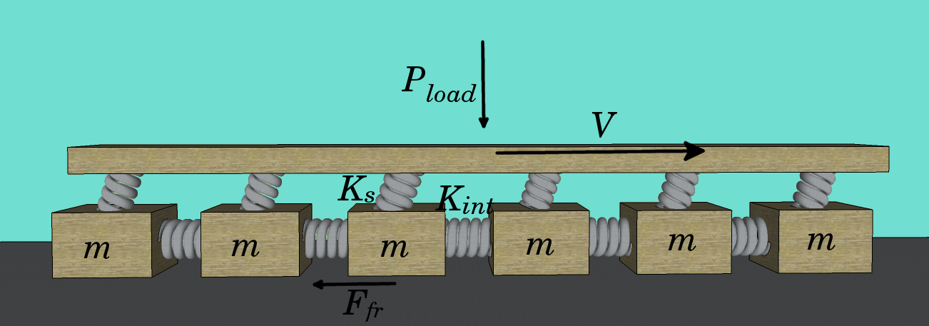
Figure 1: Schematic of the spring-block model with the notation used in the text.

As stated in the introduction, the purpose of this work is to investigate the variation of friction coefficients in the presence of structured surfaces, also taking into account material elasticity. With this in mind, we start from a one dimensional spring-block model. This model was first introduced in 1967 by Burridge and Knopoff burr in the study of the elastic deformation of tectonic plates. Despite its simplicity, the model is still used not only in this field equake1 -equake3 , but also to investigate some aspects of dry friction on elastic surfaces, e.g. the static to dynamic friction transition braun -urb , stick-slip behaviour capoz1 -sche and the role of regular patterning capoz3 .

The model is illustrated in figure 1: an elastic body, sliding along a rigid surface, is discretized in a chain of blocks of mass $m$ connected by springs of stiffness $K_{int}$, attached to a slider moving at constant velocity $v$ by means of springs of stiffness $K_{s}$ to take into account shear deformation. The surface of the sliding plane is considered as a first approximation homogeneous and infinitely rigid.

Friction between the blocks and the surface can be introduced in many ways: for example in braun it is modeled through springs that can attach and detach during motion. However, in our study we will use a classical AC friction force between blocks and surface through microscopic friction coefficients, as it is done, for example, in trom . In this way it is possible to directly introduce a pressure load as in the figure. Hence, on each block the acting forces are:

1. The shear elastic force due to the slider uniform motion, $F_{s}=K_{s}(vt+l_{i}-x_{i})$, where $x_{i}$ is the position of the block $i$ and $l_{i}$ is its rest position.

2. The internal elastic restoring force between blocks $F_{int}=K_{int}(x_{i+1}+x_{i-1}-2x_{i})$.

3. The normal force $F_{n}$, which is the total normal force divided for the number of blocks in contact with the surface.

4. A viscous force $F_{damp}=-m\gamma\dot{x_{i}}$ to account for damping effects, with $\gamma$ chosen in the underdamped regime.

5. The AC friction force $F_{fr}$: if the block $i$ is at rest, the friction force is equal and opposite to the resulting moving force, up to the threshold $F_{fr}={\mu_{s}}_{i}\;{F_{n}}$. When this limit is exceeded, a constant dynamic friction force opposes the motion, i.e. $F_{fr}={\mu_{d}}_{i}\;F_{n}$. The microscopic friction coefficients of each block, namely ${\mu_{s}}_{i}$ and ${\mu_{d}}_{i}$, are assigned through a Gaussian statistical dispersion to account for the random roughness of the surface. Thus, the probability distribution for the static coefficient is $p({\mu_{s}}_{i})=(\sqrt{2\pi}\sigma_{s})^{-1}\exp{[-({\mu_{s}}_{i}-(\mu_{s})_{m})^{2}/(2\sigma_{s}^{2})]}$, where $(\mu_{s})_{m}$ denotes the mean microscopic static coefficient and $\sigma_{s}$ is its standard deviation. The same distribution is adopted for the dynamic coefficient ( substituting subscript $d$ to $s$). The macroscopic friction coefficients, obtained through the sum of all the friction forces on the blocks, will be denoted as $(\mu_{s})_{M}$ and $(\mu_{d})_{M}$.

Hence, we have a system of equations for the block motion that can be solved numerically with a fourth-order Runge-Kutta algorithm. Since the friction coefficients of the blocks are randomly extracted at each run, the final result of any observable consists on an average of various repetitions of the simulation. Usually, we assume an elementary integration time step of $h=10^{-4}$ ms and we repeat the simulation about twenty times.

In order to relate the model to a realistic situation, we fix the macroscopic quantities, i.e. the global shear modulus $G=5$ MPa, the Young’s modulus $E=15$ MPa, the mass density $\rho=1.2$ g/cm³ (typical values for a rubber-like material with Poisson ratio $\nu=0.5$), the total length $L_{x}$, the transversal dimensions of the blocks $l_{y}$, $l_{z}$ and the number of blocks $N$. These quantities are then related to the stiffnesses $K_{int}=E\cdot(N-1)l_{z}l_{y}/L_{x}$ and $K_{s}=G\cdot l_{y}L_{x}/(l_{z}N)$, the length of the blocks $l_{x}=L_{x}/N$, and their mass $m=\rho l_{x}l_{y}l_{z}$. The default values of the parameters are specified in table 1. An example of the simulated friction force time evolution of the system with these values is shown in figure 3.

parameter	default value
shear modulus G	5 MPa
elastic modulus E	15 MPa
density $\rho$	1.2 g/cm3
total load pressure $P_{load}$	1 MPa
damping $\gamma$	10 ms-1
slider velocity $v$	0.05 cm/s
length $l_{y}$	1 cm
length $l_{z}$	0.1 cm
micro. static coeff. $(\mu_{s})_{m}$	1.0 (1)
micro. dynamic coeff. $(\mu_{d})_{m}$	0.50 (1)

Table 1: Values of the default parameters of the model. For the microscopic friction coefficients we denote in round brackets the standard deviation of their Gaussian dispersion. The total length $L_{x}$ and the number $N$ of blocks will be specified for each considered case.

II.1 Smooth surfaces

Before introducing surface patterning, as a preliminary study we show some results with the system in the standard situation of all blocks in contact. First, we show how the macroscopic friction coefficients depend on microscopic ones and longitudinal dimensions. As seen in figure 3, with $l_{x}$ fixed, the friction coefficients decrease with the number of blocks $N$ and, consequently, the overall length $L_{x}=Nl_{x}$. This effect is analogous to that seen in fracture mechanics, in which the global strength decreases with increasing element size, due to the increased statistics fbm1 fbm2 . Indeed, a reduction in width of the distribution of the microscopic $\mu_{s}$ leads, as expected, to an increase in the global static friction coefficient. This statistical argument is a possible mechanism for the breakdown of AC law, observed for example in exp1 .

The macroscopic dynamic coefficient, instead, is largely unaffected by the number of blocks, as shown in figure 3, and in any case its variation is less than $10\%$. We observe also that it is greater than the average microscopic coefficient. This is to be expected, since during the motion some blocks are at rest and, hence, the total friction force in the sliding phase has also some contributions from the static friction force (see also section II.2).

On the other hand, by varying $l_{x}$ with fixed $N$, the values of the stiffnesses $K_{s}$ and $K_{int}$ are changed and, hence, the relative weight of the elastic forces. Depending on which one prevails, the system displays two different qualitative regimes: if $K_{int}>K_{s}$, the internal forces dominates so that, when a block begins to move after its static friction threshold has been exceeded, the rupture propagates to its neighbor and a macroscopic sliding event occurs shortly after. In this case, the total friction force in the dynamic phase exhibits an irregular stick-slip behaviour, as shown, for example, in figure 3. Instead, if $K_{int}\lesssim K_{s}$, the internal forces are less influential, so that the macroscopic rupture occurs only when the static friction threshold of a sufficient number of blocks has been exceeded.

In a real material, the distance $l_{x}$ can be related to the characteristic length between asperities on the rough surface of the sliding material. Hence, the regime with a shorter $l_{x}$, implying a larger $K_{int}$, can be interpreted as a material whose asperities are close packed and slide together, while in the other limit they move independently. In the following, we will consider the regime $K_{int}>K_{s}$, which is more representative for the rubber-like parameters we have chosen with realistic length scales.

The plot of the resulting macroscopic friction coefficients as a function of the stiffnesses is shown in figure 4: the static friction coefficients is constant in the region $K_{int}>K_{s}$ and it starts to increase when the stiffnesses become comparable. This is to be expected, since by reducing the force between blocks only the force due to shear deformation remains. The dynamic friction coefficients slightly increase by reducing $K_{int}$ in both the regimes for the same reason of the static coefficients: the total force is reduced during the sliding phase and, hence, the fraction of resting blocks is increased.

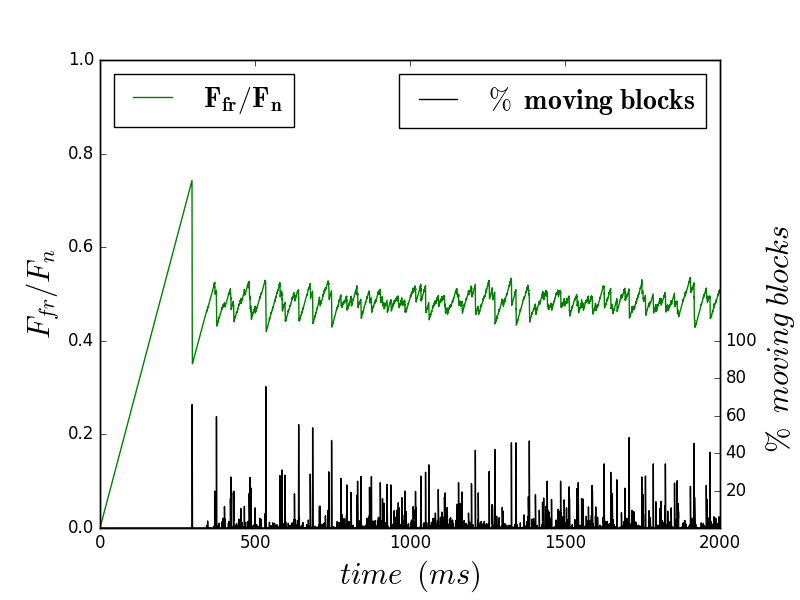
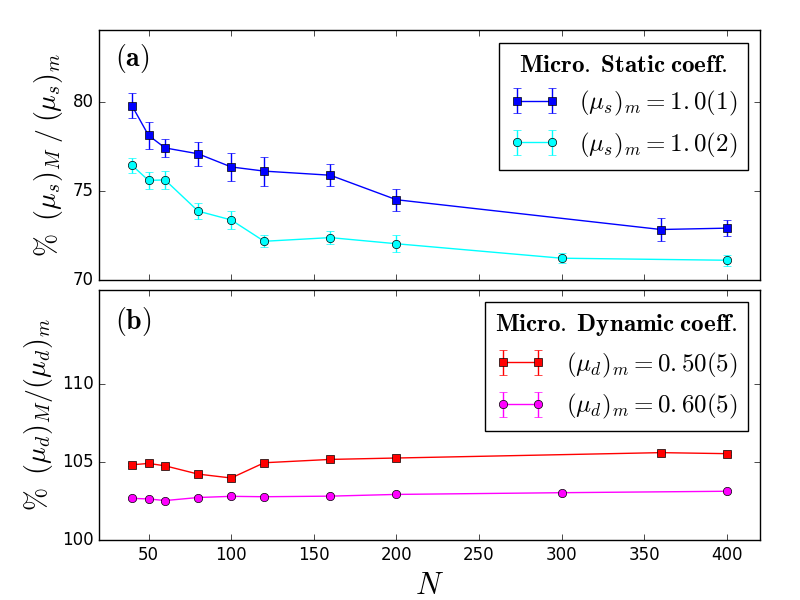
Figure 2: Plot of the total friction force normalized with the total normal load as a function of time with the default set of parameters and $L_{x}=4.0$ cm and $N=200$. We can observe the typical AC force behaviour with a linear phase up to the detachment threshold followed by a dynamic phase with an irregular stick-slip behaviour due to the randomness of the microscopic friction coefficients. From this plot we can extract for example the static friction coefficient from the first load peak and the dynamic one from the average over the dynamic phase. The plot also shows the variation in time of the number of detached blocks.

Figure 3: Macroscopic static (a) and dynamic (b) friction coefficients using the default set of model parameters as a function of material discretization $N$. The block length is fixed at $l_{x}=L_{x}/N=0.02$ cm, so that the ratio $K_{int}/K_{s}$ is also fixed. The dynamic coefficient is practically constant while the static coefficient slightly decreases. Two sets of values for the local coefficients are considered, as indicated in the legend, with the standard deviation of their Gaussian dispersion reported in round brackets. A wider statistical dispersion reduces the global static friction coefficient.

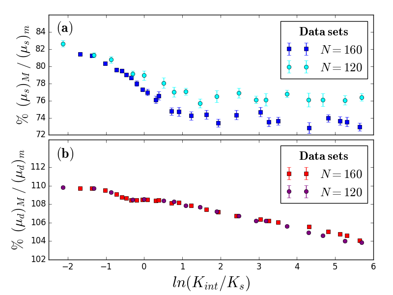
Figure 4: Macroscopic static (a) and dynamic (b) friction coefficients using the default set of parameters as a function of $K_{int}/K_{s}$ obtained by varying $l_{x}$ for set values of $N$. The dynamic coefficients increase by reducing $K_{int}$. The static coefficients instead are constant for $K_{int}>K_{s}$, and they decrease for larger $N$, as in figure 3. The static coefficients begin to increase only when the stiffnesses are comparable.

II.2 Dynamic friction coefficient

In this section, we calculate analytically the dynamic friction coefficient in the limit of $K_{int}=0$. This is useful as a further test of the program and to highlight some interesting properties of the macroscopic friction coefficient. In this limit, the blocks move independently, so that the resulting friction force can be obtained by averaging the behavior of a single block. Let us consider a single block of mass $m$, which is pulled by the slider, moving at constant velocity $v$, with an elastic restoring force of stiffness $k$. The AC friction force acts on the block, whose static and dynamic friction coefficient are ${\mu_{s}}_{i}$ and ${\mu_{d}}_{i}$ respectively. In the following, we will drop the index $i$ for simplicity.

The maximum distance $r_{0}$ between the block and the slider can be found by equating the elastic force and the static force, ${\mu_{s}}F_{n}=kr_{0}$, where $F_{n}$ is the normal force on the block. From this distance the block starts to move under the effect of the elastic force and dynamic friction force, therefore we can solve the motion equation for the position $x$ of the block:

$$\ddot{x}(t)=-\omega^{2}\;(x(t)-vt-r_{0})-{\mu_{d}}\frac{F_{n}}{m}$$ (1)

where $\omega=\sqrt{k/m}$, and $r_{0}={\mu_{s}}F_{n}/k$ is the initial distance between the block and the slider. By solving the differential equation with initial conditions $x(0)=0$, $\dot{x}(0)=0$ we obtain:

$$x(t)=\frac{v}{\omega}\;(\omega t-\sin{\omega t})+\frac{F_{n}}{k}\;({\mu_{s}}-{\mu_{d}})\;(1-\cos{\omega t})$$ (2)

$$\dot{x}(t)=v\;(1-\cos{\omega t})+\frac{\omega F_{n}}{k}\;(\mu_{s}-\mu_{d})\;\sin{\omega t}$$ (3)

The equation for the velocity (3) can be used to find the time duration $T_{d}$ of the dynamic phase. After this time the block halts and the static friction phase begins. Hence, by setting $\dot{x}(t)=0$ and solving for $t>0$, after some manipulations using trigonometric relations, we find:

$$T_{d}=\frac{2}{\omega}\Bigg{[}\pi-\arctan{\left((\mu_{s}-\mu_{d})\frac{\omega F_{n}}{kv}\right)}\Bigg{]}$$ (4)

In order to characterize the static phase, it is important to calculate the distance $\Delta r$ between the slider and the block at the time $T_{d}$, because the subsequent duration $T_{s}$ of the static phase will be determined by the time necessary for the slider to again reach the maximum distance $r_{0}$. Therefore, we must calculate $\Delta r\equiv x(T_{d})-vT_{d}-r_{0}$. After some calculations we find:

$$\Delta r=\frac{F_{n}}{k}\;(\mu_{s}-2\mu_{d})$$ (5)

Hence, if $2\mu_{d}=\mu_{s}$ the block exactly reaches the slider after every dynamic phase. If $2\mu_{d}<(>)\;\mu_{s}$ the block stops after (before) the slider position. Hence there are two regimes determined by the friction coefficients. From this we can calculate the distance required by the slider to again reach the maximum distance $r_{0}$ and, hence, the duration time $T_{s}$ of the static phase:

$$T_{s}=\frac{2F_{n}}{kv}\;(\mu_{s}-\mu_{d})$$ (6)

Now we have all the ingredients to calculate the time average of the friction force, from which the dynamic friction coefficient can be deduced. We restore the index $i$ to distinguish the microscopic friction coefficients from the macroscopic one $(\mu_{d})_{M}$. We write the time average of the friction force as the sum of the two contributions from the dynamic phase and the static one:

$$(\mu_{d})_{M}\equiv\frac{<F_{fr}>}{F_{n}}=\frac{1}{F_{n}}\left(\frac{T_{d}}{T_{tot}}{\mu_{d}}_{i}F_{n}+\frac{T_{s}}{T_{tot}}<F_{stat}>\right)$$ (7)

so that:

$$(\mu_{d})_{M}={\mu_{d}}_{i}+\frac{T_{s}}{T_{tot}}\left(\frac{<F_{stat}>}{F_{n}}-{\mu_{d}}_{i}\right)$$ (8)

where $T_{tot}=T_{d}+T_{s}$ and $F_{stat}$ is the static friction force. In the static phase the friction force is equal to the elastic force, hence, in practice, we must calculate the time average of the modulus of the distance between block and slider in the static phase, i.e. the average of $k|vt+\Delta r|$ over the time necessary for the slider to go from $\Delta r$ to $r_{0}$. For this reason, we must distinguish the two regimes depending on the sign of $\Delta r$ calculated in equation (5). After some calculations we find:

$$<F_{stat}>=\left\{\begin{array}[]{ll}F_{n}\;{\mu_{d}}_{i}\;\;\mbox{if}\;\;2{\mu_{d}}_{i}\geq{\mu_{s}}_{i}\\ \\ F_{n}\frac{({\mu_{s}}_{i}-2{\mu_{d}}_{i})^{2}+{{\mu_{s}}_{i}}^{2}}{4({\mu_{s}}_{i}-{\mu_{d}}_{i})}\;\;\mbox{if}\;\;2{\mu_{d}}_{i}<{\mu_{s}}_{i}\end{array}\right.$$ (12)

Finally, by substituting equation (12) into (8), we obtain:

$$(\mu_{d})_{M}=\left\{\begin{array}[]{ll}{\mu_{d}}_{i}\;\;\mbox{if}\;\;\;2{\mu_{d}}_{i}\geq{\mu_{s}}_{i}\\ \\ {\mu_{d}}_{i}+\frac{T_{s}}{T_{tot}}\frac{({\mu_{s}}_{i}-2{\mu_{d}}_{i})^{2}}{2({\mu_{s}}_{i}-{\mu_{d}}_{i})}\;\;\mbox{if}\;\;2{\mu_{d}}_{i}<{\mu_{s}}_{i}\end{array}\right.$$ (16)

showing that the limit case ${\mu_{d}}_{i}={\mu_{s}}_{i}/2$ of the two expressions coincides. Now, if we have $N$ non-interacting blocks, we can average the equations (16) over the index $i$ in order to calculate the macroscopic friction coefficient in terms of the mean microscopic ones, $(\mu_{s})_{m}$ and $(\mu_{d})_{m}$. Since the second term of equation (16) contains a complicated expression, this can be done exactly only numerically. Nevertheless, we can deduce that, at least in the regime of negligible $K_{int}$, (i) the resulting dynamic friction coefficient is always greater or equal to the microscopic one, and (ii) there are two regimes discriminated by the condition $2\;(\mu_{d})_{m}\gtrless(\mu_{s})_{m}$. We observe also that in the case $2\;(\mu_{d})_{m}\simeq(\mu_{s})_{m}$, owing to the statistical dispersion of the coefficients, each block could be in both the regimes, so that the final result will be an average between the two conditions of (16).

The following plot (figure 5) shows the behavior predicted by equation (16) compared with the simulations either in ideal case $K_{int}=0$, that perfectly match with the theory, and with blocks interactions, that diverge from the predictions only for $(\mu_{d})_{m}/(\mu_{s})_{m}<0.5$. This is to be expected, since the internal forces become much more influential if the blocks can move without a strong kinetic friction.

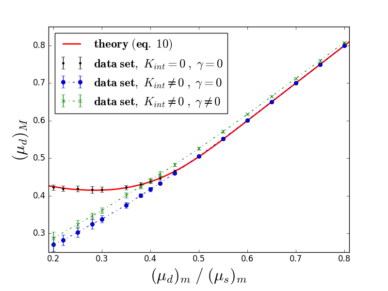
Figure 5: Macroscopic dynamic friction coefficient as a function of the microscopic one. The red curve shows the theory prediction by Eq. (16). Results of the ideal case $K_{int}=0$ are the black dots, which follow exactly the predictions. The yellow and the blue dots show the data sets with blocks interaction, with and without the damping $\gamma$, respectively. The data are obtained with the default system parameters, $N=200$ and $L_{x}=4.0$ cm.

III Structured Surfaces

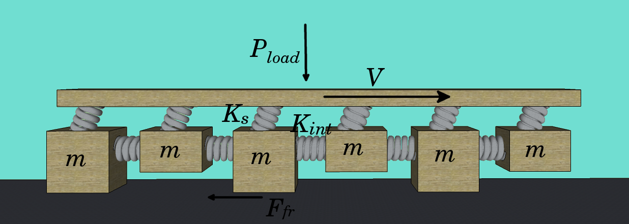
Figure 6: In order to evaluate the effect of surface structuring, we assume in the spring-block model that a number of blocks is no longer in contact with the sliding plane and is instead free to oscillate. The total pressure is maintained constant, so that the normal force on the blocks in contact increases.

III.1 First level patterning

Next, we set to zero the friction coefficients relative to some blocks in order to simulate the presence of structured surfaces on the sliding material (figure 6). We start with a periodic regular succession of grooves and pawls. This pattern has already been studied both experimentally brass snake and numerically with a slightly different model capoz3 . Our aim is therefore to first obtain known results so as validate the model.

We consider a succession of $N_{g}$ grooves of size $L_{g}$ at regular distances of $L_{g}$, so that only half of the surface is in contact with respect to previous simulations. The number of blocks in each groove is $n_{g}=N/(2N_{g})$, and $L_{g}=n_{g}L_{x}/N$. The friction coefficients of these blocks are set to zero while default values are used for the remaining ones.

Figure 7 shows that, as expected, the static friction coefficient decreases with larger grooves while the dynamic coefficient is approximately constant. In the case of small grooves, e.g. for $n_{g}\leq 2$, there is no reduction, confirming the results in capoz3 , where it is found that the static friction reduction is expected only when the grooves length is inferior to a critical length depending on the stiffnesses of the model. The critical length can be rewritten in terms of the adimensional ratio $N_{g}/N$ and, by translating it in the context of our model, we obtain $(N_{g}/N)_{cr}=2\sqrt{K_{s}/K_{int}}$. For the data set of figure 7 the critical value is $(N_{g}/N)_{cr}\simeq 0.23$ and, indeed, our results display static friction reduction for groove size whose $N_{g}/N$ is inferior to this.

The origin of this behaviour in the spring-block model can easily be understood by looking at the stress distribution on the patterned surfaces (figure 8 a): stresses at the edge of the pawls increase with larger grooves, so that the detachment threshold is exceeded earlier and the sliding rupture propagates starting from the edge of the pawls. The larger the grooves, the more stress is accumulated. Thus, for a constant number of blocks in contact, i.e. constant real contact area, the static friction coefficient decreases with larger grooves.

Next, we evaluate configurations in which the pawls and the grooves have different sizes, i.e. the fraction of surface in contact is varied. This is equivalent to changing the normal force applied to the blocks in contact, since the total normal force is fixed. We must denote these single-level configurations with two symbols, the number of blocks in the grooves $n_{g}$ as previously, but also the number of blocks in the pawls, namely $n_{p}$. When they are the same we will report only to $n_{g}$, as in figure 7. All the results obtained for the macroscopic friction coefficient are reported in table 2 and shown in figure 9.

We can observe that, for a given fraction of surface in contact, the static friction decreases for larger grooves, as in the case ${n_{p}}={n_{g}}$. However, with different ${n_{p}}$ and ${n_{g}}$ values, static friction increases when the pawls are narrower than the grooves, i.e. when the real contact area is smaller than one half.

This would appear to be in contrast with results observed previously relative to the relative groove size. However, the normal load applied to the blocks must also be taken into account: if the normal force is distributed on fewer blocks, the static friction threshold will also be greater although the driving force is increased (figure 8 b). Hence, static friction reduction due to larger grooves can be balanced by reducing the real contact area, as highlighted by results in table 2.

The interplay between these two concurrent mechanisms explains the observed behaviour of the spring-block model with single-level patterning using pawls and grooves of arbitrary size.

The dynamic friction coefficient, on the other hand, displays reduced variation in the presence of patterning, and in practice increases only when there is a large reduction of the number of blocks in contact.

Finally, we have also tested a configuration with randomly distributed grooves, i.e. half the friction coefficients of randomly chosen blocks are set to zero. This turns out to be the configuration with the smallest static friction. This can be explained by the fact that there are grooves and pawls at different length scales, so that it is easier to trigger sequences of ruptures, leading to a global weakening of the static friction. Thus, the simulations show that in general a large statistical dispersion in the patterning organization is detrimental to the static friction of a system, whilst an ordered structure is preferable in most cases.

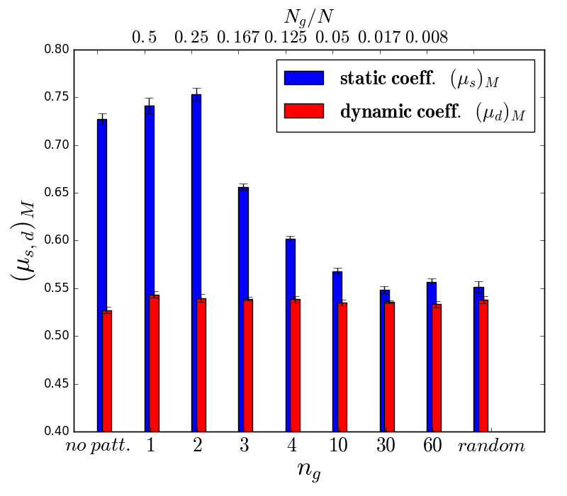
Figure 7: Static and dynamic friction coefficients for a periodic regular patterned surface as a function of number of blocks in a groove $n_{g}$. Results are obtained with the default set of parameters, $L_{x}=7.2$ cm and $N=360$, and microscopic friction coefficients $(\mu_{s})_{m}=1.0(1)$ and $(\mu_{d})_{m}=0.50(1)$. The behaviour is analogous to that observed in the literature snake .

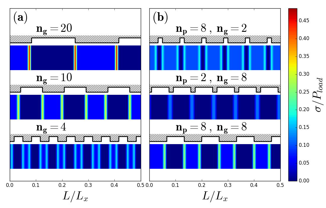
Figure 8: Normalized stress distribution $\sigma$ as a function of the longitudinal distance $L$ along the patterned surface, i.e. stress acting on each block normalized by the total applied pressure. For the three considered cases, the patterning profile is illustrated with a black line.
a) Case of regular periodic patterning for different $n_{g}$ values. For larger grooves, the stress on the blocks at the pawl edges increases.
b) Three cases varying the relative length of grooves and pawls: for small pawls, despite the larger grooves, the stress is reduced because of the increased normal load on the blocks in contact.

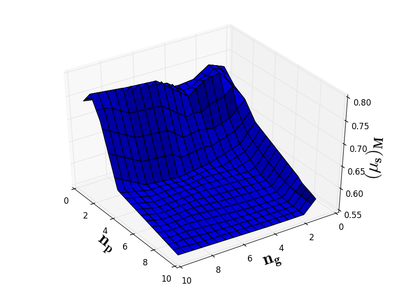
Figure 9: Plot of the static friction coefficient as a function of the size of grooves and pawls (see table 2).

III.2 Hierarchical patterning

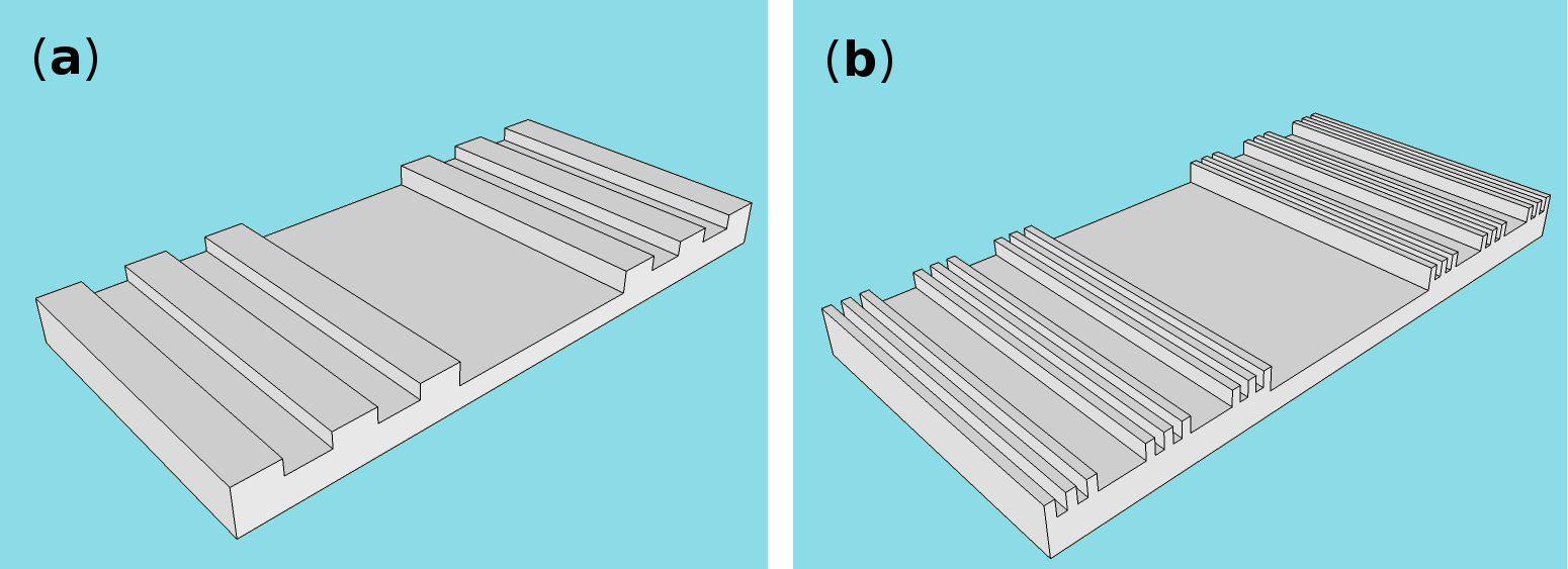
Figure 10: Example of the elementary structure of surfaces with two (a) and three (b) levels of patterning. With the notation used in the text the left configuration is denoted by $\lambda_{1}=1/3$, $\lambda_{2}=1/15$, the right one by $\lambda_{1}=1/3$, $\lambda_{2}=1/15$, $\lambda_{3}=1/75$.

We now consider grooves on different size scales, arranged in 2- and 3-level hierarchical structures, as shown in figure 10. Further configurations can be constructed with more hierarchical levels, by adding additional patterning size scales.

The configurations are identified using the ratios between the length of the grooves at level $i$ and the total length: $\lambda_{i}\equiv L_{g}^{(i)}/L_{x}$. For example, a hierarchical configuration indicated with $\lambda_{1}=1/5$, $\lambda_{2}=1/15$, $\lambda_{3}=1/120$ has three levels with groove sizes $L_{g}^{(1)}=L_{x}/5$, $L_{g}^{(2)}=L_{x}/15$, $L_{g}^{(3)}=L_{x}/120$, respectively, from the largest to the smallest. In the spring block model this implies that the number of blocks in each groove at level $i$ is $n_{g}^{(i)}=N\lambda_{i}$. For readability, these numbers will be shown in the tables. Macroscopic friction coefficients for various multi-level configurations are reported in the appendix A. The comparison of the total friction force as a function of the time between the case of a smooth surface, single level and two-levels patterning is shown in figure 11.

In general, by adding more levels of patterning (as in figure 10) the static friction coefficients increases with respect to the single-level configuration whose groove size is that of the first hierarchical level (see figure 12). This effect is due to the increased normal force on the remaining contact points, since the total normal force applied to the whole surface is constant, but it is distributed on a smaller number of blocks. This increase of the static friction becomes more significant the more the length scales of the levels are different. Indeed, if the groove size of the first level is fixed, there is a progressive reduction of the static friction as the second-level groove size increases, down to the value obtained with a single level. These trends can be clearly observed in tables 3 and 4. On the other hand, if we compare a hierarchical configuration with a single-level one with the same contact area, i.e. if we compare the results of table 2 and table 4 for the same fraction of surface in contact and the same first level size, we observe a reduction of the static friction (see figure 13).

Hence, a multi-structured surface produces an increase in static friction with respect to a single-level patterning with the same first level groove size, but a decrease with respect to that with the same real contact area. The explanation is the following: if the normal load is fixed, a structure of nested grooves allows to distribute the longitudinal forces on more points of contact on the surface, so that the static threshold will be exceeded earlier with respect an equal number of points arranged without a hierarchical structure. In other words, the hierarchical structure increases the number of points subjected to stress concentrations at the edges of the grooves.

Hence the role of the hierarchy can be twofold: if the length scale of the grooves at some level is fixed, by adding a further hierarchical level with a smaller length scale we can strengthen the static friction by reducing the number of contact points. On the other hand, among the configurations with the same fixed fraction of surface in contact, the hierarchical one has the weakest static friction, because the longitudinal stress is distributed on more points.

Moreover, the dynamic friction coefficients do not show variations greater than a few percent with respect the case of smooth surfaces, but they increase by reducing the blocks in contact and, consequently, also by adding hierarchical levels.

From all of these considerations, we can also deduce that, by increasing the number of hierarchical levels and by appropriately choosing the groove size at each level, it is possible to fine tune the friction properties of a surface, exploiting an optimal compromise between the extremal effects. Hierarchical structure is essential as it provides the different length scales needed to manipulate the friction properties of the surface.

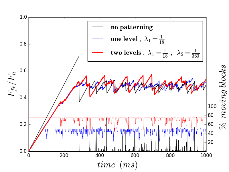
Figure 11: Comparison of the total friction force normalized with the total load for increasing levels of patterning, using the default set of parameters and $L_{x}=7.2$ cm and $N=360$. A reduction of the static friction force is observed with respect to the non patterned case. However, adding a further level, the static friction increases again, and dynamic friction displays a more evident time variation although the average is approximately the same.

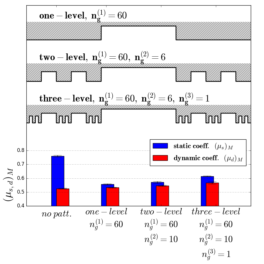
Figure 12: Static and dynamic friction coefficients obtained by adding further hierarchical levels (labeled as in table 3) but keeping fixed the first level size. For each considered case the grooves profile along the surface is shown. Results are obtained with the default set of parameters, $L_{x}=2.4$ cm, $N=120$ and microscopic friction coefficients $(\mu_{s})_{m}=1.0(1)$ and $(\mu_{d})_{m}=0.50(1)$.

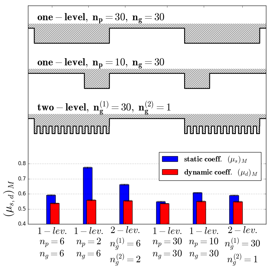
Figure 13: Comparison of static and dynamic friction coefficients for some cases of one- and two-level patterning with the default parameters, $L_{x}=7.2$ cm, $N=360$. For each considered case the groove profile along the surface is shown. With two levels the static friction is reduced with respect to the corresponding one-level case with same contact area and same size of the largest grooves.

IV Conclusions

In this paper, we have investigated how the macroscopic friction coefficients of an elastic material are affected by a multilevel structured surface constructed with patterning at different length scales. Our results were obtained by means of numerical simulations using a one-dimensional spring-block model, in which friction is modeled using the classical AC friction force with microscopic friction coefficients assigned with a Gaussian statistical distribution. System parameters were chosen in such a way as to be as close as possible to realistic situations for rubber-like materials sliding on a rigid homogeneous plane.

Tests were initially performed for a smooth surface: in this case the model predicts that the friction coefficients slightly decrease with the number of asperities in contact, i.e. the number of blocks, an effect that can be ascribed to statistical dispersion. The friction coefficients also decrease if the asperities are close-packed (i.e. the blocks distance is shorter), because their slipping occurs in groups and the local stress is increased .

The presence of patterning was then simulated by removing contacts (i.e. friction) at selected locations, varying the length of the resulting pawls and grooves and the number of hierarchical levels. The model predicts the expected behaviour for a periodic regular patterning, correctly reproducing results from experimental studies.

We have shown that in order to understand the static friction behaviour of the system in presence of patterning two factors must be taken into account: the length of the grooves and the discretization of the contacts (i.e. number of blocks in contact). The longitudinal force acting on the pawls increases with larger grooves, so that a smaller global static coefficient can be expected. However, if the fraction of surface in contact is small, the friction threshold increases and so does the global static friction. Single-level patterning frictional behaviour can be understood in terms of these mechanisms.

In a multi-level patterned structure, the hierarchy of different length scales provides a solution to reduce both the effects. If at any level of the hierarchy the grooves are so large that the static friction is severely reduced, a further patterning level, whose typical length scales are definitely smaller, can enhance it again, since with a reduced number of contact points the static threshold is increased.

On the other hand, if we compare the configurations with the same fraction of surface in contact, the hierarchical structure has the weakest static friction, since it increases the number of points at the edges between pawls and grooves and, consequently, the fraction of surface effectively subjected to longitudinal stress concentrations. Thus, a hierarchical structure can be used to construct a surface with a small number of contact points but with reduced static friction.

These results indicate that exploiting hierarchical structure, global friction properties of a surface can tuned arbitrarily acting only on the geometry, without changing microscopic friction coefficients. To achieve this, it is essential to provide structuring at various different length scales.

In this study, the effect of different length scales and structure has been studied for constant material stiffnesses and local friction coefficients, but in future we aim to verify the existence of universal scaling relations by changing the system size parameters, and to analyze the role of the mechanical properties, e.g. for composite materials or graded frictional surfaces. Also, a natural extension of this study is to consider two- or three-dimensionally patterned surfaces, allowing a more realistic description of experimental situations and a larger variety of surface texturing possibilities. These issues will be explored in future works.

Appendix A Tables

${n_{p}}$	${n_{g}}$	$S/S_{tot}$	$(\mu_{s})_{M}$	$(\mu_{d})_{M}$
no patt.		1	0.727 (7)	0.527 (3)
1	1	1/2	0.741 (8)	0.543 (3)
2	2	1/2	0.753 (6)	0.540 (4)
3	3	1/2	0.656 (4)	0.539 (2)
4	4	1/2	0.602 (3)	0.539 (3)
10	10	1/2	0.568 (4)	0.535 (3)
20	20	1/2	0.563 (4)	0.536 (3)
30	30	1/2	0.543 (4)	0.535 (2)
60	60	1/2	0.557 (4)	0.533 (3)
1	2	1/3	0.755 (7)	0.555 (5)
2	4	1/3	0.722 (9)	0.554 (4)
4	8	1/3	0.599 (2)	0.545 (4)
10	20	1/3	0.593 (4)	0.545 (3)
20	40	1/3	0.566 (4)	0.542 (4)
1	3	1/4	0.733 (9)	0.563 (8)
2	6	1/4	0.775 (5)	0.559 (5)
5	15	1/4	0.649 (4)	0.554 (4)
10	30	1/4	0.607 (3)	0.551 (5)
1	4	1/5	0.729 (10)	0.567 (7)
2	8	1/5	0.780 (7)	0.564 (4)
4	16	1/5	0.684 (6)	0.561 (4)
12	48	1/5	0.602 (4)	0.548 (5)
1	8	1/9	0.744 (13)	0.587 (8)
2	16	1/9	0.810 (7)	0.585 (7)
2	1	2/3	0.713 (13)	0.534 (3)
4	2	2/3	0.624 (9)	0.534 (2)
8	4	2/3	0.568 (4)	0.532 (2)
20	10	2/3	0.547 (3)	0.530 (2)
40	20	2/3	0.541 (2)	0.531 (2)
3	1	3/4	0.699 (4)	0.532 (2)
6	2	3/4	0.586 (2)	0.531 (2)
15	5	3/4	0.548 (2)	0.529 (2)
30	10	3/4	0.554 (3)	0.528 (2)
4	1	4/5	0.663 (3)	0.531 (3)
8	2	4/5	0.568 (2)	0.530 (1)
16	4	4/5	0.544 (2)	0.528 (1)
48	12	4/5	0.548 (3)	0.527 (2)
8	1	8/9	0.602 (2)	0.528 (2)
16	2	8/9	0.545 (2)	0.528 (2)

Table 2: Table of the macroscopic friction coefficients for one level patterning configuration, with the default set parameters, $N=360$ and $L_{x}=7.2$ cm. We denote with ${n_{p}}$ and ${n_{g}}$ the number of blocks in each pawl and groove respectively. The column $S/S_{tot}$ reports the fraction of the blocks still in contact with the surface, i.e. the real area contact.

$n_{g}^{(1)}$	$n_{g}^{(2)}$	$n_{g}^{(3)}$	$S/S_{tot}$	$(\mu_{s})_{M}$	$(\mu_{d})_{M}$
8			8/15	0.575 (7)	0.531 (5)
8	1		4/15	0.617 (8)	0.544 (4)
8	2		4/15	0.597 (7)	0.545 (6)
24			3/5	0.569 (5)	0.529 (3)
24	1		3/10	0.598 (9)	0.538 (4)
24	2		3/10	0.594 (8)	0.538 (4)
24	8		2/5	0.571 (5)	0.536 (4)
24	8	1	1/5	0.628 (5)	0.550 (9)
24	8	2	1/5	0.621 (5)	0.551 (9)
40			2/3	0.565 (4)	0.525 (4)
40	1		1/3	0.608 (4)	0.532 (5)
40	2		1/3	0.588 (4)	0.533 (5)
40	8		2/5	0.573 (4)	0.534 (5)
40	8	1	1/5	0.599 (5)	0.548 (7)
40	8	2	1/5	0.603 (7)	0.547 (7)

Table 3: Table of the macroscopic friction coefficients for some cases of two and three levels patterning, with the default set parameters, $N=120$ and $L_{x}=2.4$ cm. The first three columns show the numbers $n_{g}^{(i)}$, the blocks in the grooves at level $i$, in order to identify the configuration. The column $S/S_{tot}$ reports the fraction of the blocks still in contact with the surface, i.e. the real area contact.

$n_{g}^{(1)}$	$n_{g}^{(2)}$	$n_{g}^{(3)}$	$S/S_{tot}$	$(\mu_{s})_{M}$	$(\mu_{d})_{M}$
6			1/2	0.592 (5)	0.536 (2)
6	1		1/4	0.662 (4)	0.555 (5)
10			1/2	0.568 (4)	0.535 (3)
10	1		1/4	0.614 (7)	0.552 (4)
10	2		1/4	0.603 (4)	0.548 (2)
20			1/2	0.563 (4)	0.536 (3)
20	1		1/4	0.574 (5)	0.550 (4)
20	2		1/4	0.573 (3)	0.551 (2)
30			1/2	0.543 (4)	0.535 (2)
30	1		1/4	0.591 (3)	0.549 (4)
30	2		1/4	0.601 (3)	0.550 (4)
60			1/2	0.557 (4)	0.533 (3)
60	2		1/4	0.581 (5)	0.546 (3)
60	6		1/4	0.610 (2)	0.547 (3)
60	6	1	1/8	0.653 (7)	0.568 (5)
60	10		1/4	0.571 (7)	0.546 (4)
60	10	1	1/8	0.615 (4)	0.567 (8)

Table 4: Macroscopic friction coefficients for some cases of two- and three-level patterning, using the default set parameters, $N=360$ and $L_{x}=7.2$ cm. The first three columns show the numbers $n_{g}^{(i)}$, i.e. the number of blocks in the grooves at level $i$, in order to identify the configuration. The column $S/S_{tot}$ reports the fraction of surface in contact.

References

- (1) B.N.J. Persson, Sliding Friction - Physical principles and application, in Nanoscience and Technology, Springer-Verlag Berlin Heidelberg (2000)
- (2) Y. Katano, K. Nakano, M. Otsuki, H. Matsukawa, Novel Friction Law for the Static Friction Force based on Local Precursor Slipping, Sci. Rep. 4 (2014) 6324
- (3) Z. Deng, A. Smolyanitsky, Q. Li, X.Q. Feng, R.J. Cannara, Adhesion-dependent negative friction coefficient on chemically modified graphite at the nanoscale, Nature Materials 11 (2012) 1032
- (4) A. Vanossi, N. Manini, M. Urbakh, S. Zapperi, E. Tosatti, Colloquium: Modeling friction: From nanoscale to mesoscale, Rev. Mod. Phys. 85 (2013) 529
- (5) M. Nosonovsky, B. Bhushan, Multiscale friction mechanisms and hierarchical surfaces in nano- and bio-tribology, Mater. Sci. Eng. R 58 (2007) 162
- (6) M. Nosonovsky, B. Bhushan, Multiscale Dissipative Mechanisms and Hierarchical Surfaces, Springer-Verlag Berlin Heidelberg (2008)
- (7) K. Autumn, Y. Liang, T. Hsieh, W. Zesch, W.-P. Chan, T. Kenny, R. Fearing, R.J. Full, Adhesive force of a single gecko foot-hair, Nature 405 (2000) 681
- (8) B. Bhushan, Adhesion of multi-level hierarchical attachment systems in gecko feet, J. Adhesion Sci. Technol. 21 (2007) 1213
- (9) T.W. Kim, B. Bhushan, Effect of stiffness of multi-level hierarchical attachment system on adhesion enhancement, Ultramicroscopy 107 (2007) 902
- (10) M. Varenberg, N. M. Pugno, S.N. Gorb, Spatulate structures in biological fibrillar adhesion, Soft Matter 6 (2010) 3269
- (11) N.M. Pugno, E. Lepore, S. Toscano and F. Pugno, Normal Adhesive Force-Displacement Curves of Living Geckos, The Journal of Adhesion, 87 (2011) 11
- (12) E. Lepore, N.M. Pugno, Observation of optimal gecko’s adhesion on nanorough surfaces, BioSystems 94 (2008) 218
- (13) A.E. Filippov, S.N. Gorb, Spatial model of the gecko foot hair: functional significance of highly specialized non-uniform geometry, Interface Focus 5 (2015) 20140065
- (14) M. Urbakh, E. Meyer, Nanotribology: The renaissance of friction, Nature Materials 9 (2010) 8
- (15) R. Guerra, U. Tartaglino, A. Vanossi, E. Tosatti, Ballistic nanofriction, Nature Materials 9, (2010) 634
- (16) B.J. Albers, T.C. Schwendemann, M.Z. Baykara1, N. Pilet1, M. Liebmann, E.I. Altman, U.D. Schwarz, Three-dimensional imaging of short-range chemical forces with picometre resolution, Nature Nanotech. 4 (2009) 307
- (17) S. Derler, L.C. Gerhard, Tribology of Skin: Review and Analysis of Experimental Results for the Friction Coefficient of Human Skin, Tribol. Lett. 45 (2012) 1
- (18) A. Singh, K.Y. Suh, Biomimetic patterned surfaces for controllable friction in micro- and nanoscale devices, Micro and Nano Systems Lett. 1 (2013)
- (19) A. Filippov, V.L. Popov, S.N. Gorb, Shear induced adhesion: Contact mechanics of biological spatula-like attachment devices, Jour. Theo. Bio. 276 (2011) 126
- (20) C. Greiner, M. Schafer, U. Pop, P. Gumbsch, Contact splitting and the effect of dimple depth on static friction of textured surfaces, Appl. Mater. Interfaces 6 (2014) 7986
- (21) M.J. Baum, L. Heepe, E. Fadeeva, S.N. Gorb, Dry friction of microstructured polymer surfaces inspired by snake skin, Beilstein J. Nanotechnol. 5 (2014) 1091
- (22) R. Burridge and L. Knopoff, Model and theoretical seismicity, Bull. Seismol. Soc. Am. 57 (1967) 341
- (23) S.R. Brown, C.H. Scholz, J.B. Rundle, A simplified spring-block model of earthquakes, Geophys. Res. Lett. 18 (1991) 2
- (24) J.M. Carlson, J.S. Langer, B.E. Shaw, Dynamics of earthquake faults , Rev. Mod. Phys. 66 (1994) 657
- (25) Y. Bar Sinai, E.A. Brener, E. Bouchbinder, 2012 Slow rupture of frictional interfaces, Geophys. Res. Lett. 39 (2012) 3
- (26) O.M. Braun, I. Barel, M. Urbakh, Dynamics of Transition from Static to Kinetic Friction, Phys. Rev. Lett. 103 (2009) 194301
- (27) S. Maegawa, A. Suzuki, K. Nakano, Precursors of Global Slip in a Longitudinal Line Contact Under Non-Uniform Normal Loading, Tribol. Lett. 38 (2010) 3
- (28) J. Trømborg, J. Scheibert, D.S. Amundsen, K. Thøgersen, A. Malthe-Sørenssen, Transition from Static to Kinetic Friction: Insights from a 2D Model, Phys. Rev. Lett. 107 (2011) 074301
- (29) E. Bouchbinder, E.A. Brener, I. Barel, M. Urbakh, Slow Cracklike Dynamics at the Onset of Frictional Sliding, Phys. Rev. Lett. 107 (2011) 235501
- (30) R. Capozza and M. Urbakh, Static friction and the dynamics of interfacial rupture, Phys. Rev. B 86 (2012) 085430
- (31) R. Capozza, S.M. Rubinstein, I. Barel, M. Urbakh, J. Fineberg, Stabilizing stick-slip friction, Phys. Rev. Lett. 107 (2011) 024301
- (32) N.M. Pugno, Q. Yin, X. Shi, R. Capozza, A generalization of the Coulomb’s friction law: from graphene to macroscale, Meccanica 48 (2013) 8
- (33) J. Scheibert, D.K. Dysthe, Role of friction-induced torque in stick-slip motion, EPL 92 (2010) 5
- (34) R. Capozza, N.M. Pugno, Effect of Surface Grooves on the Static Friction of an Elastic Slider, Tribol. Lett. 58 (2015) 35
- (35) S. Pradhan, A. Hansen, B. Chakrabarti, Failure processes in elastic fiber bundles, Rev. Mod. Phys. 82 (2010) 499
- (36) N.M. Pugno, F. Bosia, T. Abdalrahman, Hierarchical fiber bundle model to investigate the complex architecture of biological materials, Phys. Rev. E 85 (2012), 011903