On Shared Rate Time Series for Mobile Users
in Poisson Networks

Abstract

This paper focuses on modeling and analysis of the temporal performance variations experienced by a mobile user in a wireless network and its impact on system-level design. We consider a simple stochastic geometry model: the infrastructure nodes are Poisson distributed while the user’s motion is the simplest possible i.e., constant velocity on a straight line. We first characterize variations in the SNR process, and associated downlink Shannon rate, resulting from variations in the infrastructure geometry seen by the mobile. Specifically, by making a connection between stochastic geometry and queueing theory the level crossings of the SNR process are shown to form an alternating renewal process whose distribution can be completely characterized. For large/small SNR levels, and associated rare events, we further derive simple distributional (exponential) models. We then characterize the second major contributor to variation, associated with changes in the number of other users sharing infrastructure. Combining these two effects, we study what are the dominant factors (infrastructure geometry or sharing number) given mobile experiences a very high/low shared rate.These results are then used to evaluate and optimize the system-level Quality of Service (QoS) and system-level capacity to support mobile users sharing wireless infrastructure; including mobile devices streaming video which proactively buffer content to prevent rebuffering and mobiles which are downloading large files. Finally, we use simulation to assess the fidelity of this model and its robustness to factors which are presently taken into account.

I Introduction

The primary aim of this paper is to model and study the temporal capacity variations experienced by wireless users moving through space. These are driven by geometric variations in the spatial and environmental relationships (associations) to the infrastructure, the presence of other users, as well as random fluctuations intrinsic to wireless channels, e.g., fast fading. Our focus on temporal variability should be contrasted with the extensive work characterizing spatial variability as seen by randomly located users, e.g., through metrics such as coverage probability, spatial density of throughput, 90% quantile rate, “edge” capacity, spectral efficiency, etc. Although space and time may be related through averages (when ergodicity holds), the temporal characteristics of the stochastic processes modeling a mobile’s capacity variations are relatively unexplored beyond correlation analysis and of great practical interest.

Indeed, an increasing volume of data traffic is generated by wireless devices while moving, e.g., 20-30% of cellular data is generated during commute hours, [1]. In the future, with increasing use of public transportation and/or the emergence of driverless cars, this volume could grow substantially. The Quality of Service/Experience (QoS/E) seen by such users can be highly dependent on the capacity variations they see as they move through space. This is particularly the case for applications that operate over longer time scales, e.g., video/audio streaming, navigation/augmented reality, and real-time services, which may not be able to smooth substantial capacity variation through buffering, but also for the opportunistic transfers of large files over heterogeneous networks, e.g., WIFI offloading. More broadly, increases in wireless network capacity have been achieved through heterogeneous network densification leveraging technologies providing different coverage-throughput trade offs, e.g., cellular (macro, pico, femto cells), WIFI and perhaps, in the future, mmWave access points. Characterizing and managing the capacity variations mobile users would see across such networks is a challenging but important problem towards understanding the efficiency and performance offloading/onloading based services.

Related work. There is a rich literature on modeling spatial capacity variability in wireless infrastructure for a randomly located users. Of particular relevance is that based on stochastic geometry, which captures the effect of the variability in base station locations, as well as the variability in the environment through shadowing, and in the channel through fading, see e.g. [2] for a survey on the matter. By contrast work studying the temporal capacity variations for a user on the move in a cellular network is limited.

There is also significant related work on Delay-Tolerant Networks (DTN). This literature considers mobile nodes, where the contact duration and the inter-contact time are defined and empirically measured from real traces [3], [4] as well as through mobility models [5]. In addition to mobility induced inter-contact processes, [6] considers other factors like user availability. However, this work is in the context of opportunistic ad-hoc communication networks where a set of mobile nodes are moving under different mobility patterns. Our focus is on studying the continuous-parameter stochastic process experienced by a tagged mobile user traversing a static pattern of nodes modeling the wireless infrastructure.

There certainly is a lot of interest in studying how to design networks to better address the needs of mobile users or to leverage user mobility for the offloading/onloading traffic. For example [7] studies how user mobility patterns and users perceived QoS might drive the selection of macro-cell upgrades. The work in [8] examines the effectiveness of algorithms for optimizing offloading to a set of spatially distributed WIFI APs. The work in [9] evaluates how proactive knowledge of capacity variations could be used in designing new models for video delivery. These works exemplify applications and engineering problems which depend critically on the temporal capacity variability that mobile users would experience, but do not directly address the characteristics of such processes.

Key Questions. Two primary sources of temporal variation in a mobile’s capacity are the SNR, i.e., associated with changes in the users geometric relationship to the infrastructure, and the sharing number, i.e., the number of other mobiles sharing the resource. Our goal in this paper is to study the relative impacts these have on mobile users’ QoS/E. In this setting several basic questions arise:

1. Characterization of the SNR process. As a mobile user moves through a wireless network infrastructure associating with the closest node, its SNR process and thus associated peak rate (i.e., without accounting for sharing) will experience peaks and valleys. What is the intensity of peaks and valleys? Does it match the rate of cell boundary crossings? Given an SNR threshold, can one characterize the temporal characteristics of the on/off level crossing process associated with being above and below the threshold, i.e., the coverage and outage durations?

2. Characterization of the sharing number process. Assuming a population of other users sharing the network, what are the characteristics of the sharing number process seen by a mobile? If the network is shared by heterogeneous users, i.e., static, pedestrian, and users on public transport and/or a road system, how will this bias what they see?

3. Smoothness of the effective rate process. How smooth is the bit rate obtained by the mobile seen as a function of time? How often does this rate incur discontinuities, trend changes, large jumps or other phenomena negatively impacting real time applications?

4. Characterization of rare events. Conditional on a rare event, i.e., very poor or very good user rate, what is the relative contribution of the user’s location vs network congestion? Can one characterize the time scales for rare event occurrences?

5. Applications to QoE. What are the implications of the temporal capacity variations mobiles’ see on their application-level QoE and system-level performance, e.g., acceptable density of video streaming users, or download delays of large files?

To the best of our knowledge the analysis of the SNR and shared rate processes for Poisson wireless infrastructure developed in this paper is new and provides a first order answer to these basic questions. While our models are simplified they should be viewed as a first, and necessary, step towards characterizing temporal variability in more complex random structures, e.g., SINR variations which in this paper are only explored via simulation for comparison to SNR process characteristics. Generalizations to SINR processes would be desirable, particularly for systems operating in the interference limited regime. Such extensions may be tractable based on results known for shot noise fields (see [2], Volume 1), yet are beyond the scope of this paper.

Contributions and Organization. Section II introduces the basic model studied in this paper. We consider a tagged user moving at a fixed velocity along a straight line through a shared wireless network such that: (a) the access points/base stations are a realization of a Poisson point process; (b) other users sharing the network also form a Poisson (or possibly Cox) point process; (c) all users associate with the closest base station; (d) resources are shared equally with other users sharing the network; (e) a standard distance based path loss is used with neither shadowing nor fading. Our goal is to characterize the shared rate process seen by the tagged user by studying the SNR and sharing number processes.

In Section III we present our results on the SNR process, including the intensity of peaks and valleys and, given a SNR threshold, we provide a a complete characterization of the on/off level crossing process as an alternating-renewal process. Equivalently, this characterizes the durations for coverage/outage events seen by the mobile. Interestingly this is achieved by establishing a connection between the time-varying geometry seen by the mobile user and an associated queueing process. We then provide asymptotics for the likelihood of high and low SNR, and show that, after appropriate rescaling, the time intervals between up crossings are exponential. Which verifies the “rarity hence exponentiality” principle [10, 11] for such events.

Section IV provides a detailed discussion of the sharing number process, i.e., the number of other users which are covered, i.e., meet an SNR threshold, and share infrastructure nodes with the tagged user. The process is somewhat complex and not independent of the SNR process; so we introduce a simpler bounding process which is used in Section V to characterize the shared rate process seen by our mobile. In particular we show that rare events associated with high shared rates, are associated with high SNR (i.e., mobile’s proximity to base stations) with no other users sharing the resources. Similarly low shared rates, arise when mobiles are far from the base station, and there is a number of sharing users inversely proportional to the low rate in question. We also provide an asymptotic characterization for the re-scaled interarrival times associated with upcrossings.

In Section VI we present a discussion of discrete event simulation results which are used to assess the robustness of this model to perturbations that were not yet taken into account in the analysis. For example the relative impact of variability associated with the changing geometry (proximity of base stations) seen by a mobile versus that associated with channel variability due to channel fades.

In Section VII we leverage our results to evaluate the QoS experienced by mobile users in two concrete scenarios. First we consider the delivery of streaming video to mobile users which are able to store future video frames to prevent rebuffering. The primary question addressed is about the maximal density of such users which can be supported while ensuring that in the long term no rebuffering is required. Our second application considers the distribution for the delays experienced by a mobile user attempting to download a large file. These two examples give a system-level view on the performance that mobile users would see when downloading large files opportunistically via some WIFI infrastructure.

Section VIII briefly discusses some important extensions of our results to the case of heterogeneous wireless infrastructures and the case where the locations of mobile users follow a Cox process associated with a road network. The results show how heterogeneous technologies impact the temporal variations in the mobile users SNR process. The results also show how a mobile user on a roadway is likely to see poorer performance than a stationary or pedestrian user. Section IX concludes the paper.

II System Model

Consider an infrastructure based wireless network consisting of nodes e.g., base stations/Wifi hotspots, denoted through locations on the Euclidean plane. The configuration of the nodes is assumed to be a realization of Poisson point process $\Phi=\{X_{1},X_{2},..\}$ in $\mathbb{R}^{2}$ with intensity $\lambda$. We consider a tagged user moving at a fixed velocity $v$ along a straight line starting from the origin at time $t=0$. The mobile user shares the network with other (static) users spatially distributed according to another independent Poisson point process of intensity $\xi$.

All users associate with the closest infrastructure node. For each $X_{i}\in\Phi$ one can define a set of locations which are closer to $X_{i}$ than any other point in $\Phi\setminus{X_{i}}$. This is a convex polygon known as the Voronoi cell associated with $X_{i}$ [2]. The collection of such cells forms a tessellation of the plane called the Voronoi tessellation see e.g., Fig.1. Thus, all the users located within the Voronoi cell of node $X_{i}$ associate with $X_{i}$.

Let $(X(t),t\geq 0)$, denote the random process where, $X(t)\in\Phi$ is the closest node to the mobile user at time $t$. Let $(L(t),t\geq 0)$ be the process denoting the distance from the mobile user to its closest node.

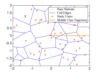
Figure 1: Mobile user motion in a sample of the Poisson cellular network.

We consider downlink transmissions and assume that all nodes transmit at a fixed power $p$. Based on the classical power law path loss model and in the absence of fading and shadowing, the Signal-to-Noise Ratio (SNR) process of the mobile user is

$$\mbox{SNR(t)}=\frac{pL(t)^{-\beta}}{w},~{}~{}\mbox{for}~{}~{}\beta>2,~{}~{}t\geq 0,$$ (1)

where $w$ denotes the noise power.

We will assume that the users are only served if their SNR exceeds a given threshold $\gamma$. It follows from (1) that a user is served if it is within a distance $r_{\gamma}=(\frac{p}{w\gamma})^{1/\beta}$ from the closest node. We refer to $r_{\gamma}$ as the radius of coverage. Note that a user may hence associate with a node but not be served.

The Shannon rate process, $(R^{(\gamma)}(t),t\geq 0)$, seen by the mobile user is directly determined by the SNR process through the relation:

$$R^{(\gamma)}(t)=\begin{cases}a\log\left(1+{\mathrm{SNR}}(t)\right)&\text{if}~{}~{}L(t)\leq r_{\gamma},\\ 0~{}~{}&\text{otherwise},\end{cases}$$ (2)

where $a$ is a constant depending on the available bandwidth.

We assume that each node shares its resources equally among the users it serves (e.g. through some time sharing scheme). We define the sharing number process $(N^{(\gamma)}(t),t\geq 0)$, where $N^{(\gamma)}(t)$ is the number of static users the node associated with the mobile user serves provided that it is itself served, and 0 if the mobile user is not served. In other words, if the mobile user is served by its closest node $X(t)$ at time $t$, it shares the resources with $N^{(\gamma)}(t)$ static users. Directly determined by the sharing number, the sharing factor $(F^{(\gamma)}(t),t\geq 0)$, is defined by:

$$F^{(\gamma)}(t)=\frac{1}{1+N^{(\gamma)}(t)}.$$ (3)

Finally, the shared rate process seen by the mobile user $(S^{(\gamma)}(t),t\geq 0)$, is given by

$$S^{(\gamma)}(t)=R^{(\gamma)}(t)\times F^{(\gamma)}(t).$$ (4)

Our aim is to characterize this process. In the next two sections, we first study the two underlying processes namely: (1) the SNR process $(\mbox{SNR}(t),t\geq 0)$ and its level sets, and (2) the Sharing number process $(N^{(\gamma)}(t),t\geq 0)$.

In the sequel, for any stationary random process say for e.g., $(S^{(\gamma)}(t),t\geq 0)$, $S^{(\gamma)}$ represents a random variable with distribution equal to the stationary distribution of this process.

A summary of the key notation is provided in the Table I.

Symbol	Definition
$\Phi,\lambda$	Poisson point process of nodes and its intensity
$\xi$	Intensity of mobile users
$p$	Constant power transmitted by nodes
$(X(t),t>0)$	Random process denoting the closest node to the mobile
$(L(t),t>0)$	Random process denoting the distance to the closest node
$(\mbox{SNR}(t),t>0)$	Signal-to-Noise ratio random process
$(C^{(\gamma)}(t),t>0)$	Signal-to-Noise ratio level crossing process
$(R^{(\gamma)}(t),t>0)$	Shannon rate random process
$(N^{(\gamma)}(t),t>0)$	Random process denoting the number of users sharing
$(S^{(\gamma)}(t),t>0)$	Shared rate random process
$\gamma$	Threshold on signal-to-noise ratio
$r_{\gamma}$	Radius of coverage for threshold $\gamma$

TABLE I: Table of Notation.

III Characterization of the SNR process

This section is structured as follows: we start by considering the on-off coverage structure of the SNR process and then study in more detail the characteristics of its fluctuations. We then analyze the scale of the inter-occurrence times of certain rare events.

III-A Analysis of the SNR Level Crossing Process

A first order question is whether the mobile is covered or not. To that end we define the SNR level crossing process as follows:

Definition 1.

Given an SNR threshold $\gamma$, the SNR level crossing process $(C^{(\gamma)}(t),t\geq 0)$ is defined as $C^{(\gamma)}(t)=\bm{1}(\mbox{SNR}(t)\geq\gamma)$ as shown in Fig 2.

Clearly this is an on-off process, where the on and off periods correspond to the coverage and outage periods respectively. The process alternates between “on” intervals of length $(B^{(\gamma)}_{n},n\geq 1)$ and “off” intervals of length $(I^{(\gamma)}_{n},n\geq 1)$ as depicted in Fig. 2. We also define the sequence of SNR up-crossing times $(T^{(\gamma)}_{n},n\geq 1)$ for a given threshold $\gamma$. Let $V^{(\gamma)}\sim T^{(\gamma)}_{n}-T^{(\gamma)}_{n-1}$ be a random variable whose distribution is that associated with up-crossing inter arrivals as illustrated in Fig. 2.

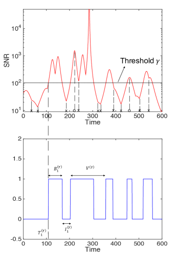
Figure 2: Level crossings of the SNR process as an On-Off process (bottom) and the point process of its local maxima $\chi$, denoted by “o” on the $x$ axis, together with edge crossings, denoted by “$\times$” (top).

In order to characterize the SNR level crossing process, we establish a connection between the time-varying geometry seen by the mobile user and an associated queueing process.

Let $D^{(\gamma)}(t)$ denote the closed disc of radius $r_{\gamma}$ centered on the mobile user’s location at time $t$. This closed disc follows the mobile user’s motion along the straight line. Let $K^{(\gamma)}(t)=|\Phi\cap D^{(\gamma)}(t)|$ denote the number of nodes in the disc.

The following theorem provides a simple characterization of $(K^{(\gamma)}(t),t\geq 0)$ which in turn will help studying the SNR level crossing process.

Theorem 1.

The process $(K^{(\gamma)}(t),t\geq 0)$ is equivalent to that modeling the number of customers in an $M/GI/\infty$ queue with arrival rate $\lambda^{({\gamma})}=2r_{\gamma}v\lambda$ and i.i.d. service times with density

$$f_{W^{(\gamma)}}(s)=\begin{cases}\frac{v^{2}s}{2r_{\gamma}\sqrt{4r_{\gamma}^{2}-v^{2}s^{2}}}~{}~{}&\text{for}~{}s\in[0,2r_{\gamma}/v],\\ 0~{}~{}&\text{otherwise}.\end{cases}$$ (5)

Proof.

The entry of a node into the closed disc $D^{(\gamma)}(t)$ can be viewed as an arrival to the queue. The amount of time spent by the node in $D^{(\gamma)}(t)$ corresponds to its service time and thus the exit from $D^{(\gamma)}(t)$ its departure from the queue.

We first show that the arrival process to the disc and thus the queue, is Poisson. We begin by proving that the arrival process has independent and stationary increments.The probability that there is an arrival in the next $\epsilon$ seconds is the probability that there is a node in the area $A^{(\gamma)}_{\epsilon}={2r_{\gamma}v\epsilon}$ as depicted in Fig. 3. Since nodes are distributed according to a homogeneous Poisson point process of intensity $\lambda$, the number of nodes in any closed set of area $b$ follows the Poisson distribution with parameter $\lambda b$. Thus, for any $\epsilon>0$, the increments in the arrival process have the same distribution. Also, the number of nodes in any two disjoint closed sets are independent. Thus, the arrival process has independent stationary Poisson increments. For a small value of $\epsilon$, the probability that there is a single arrival is given by $\lambda A^{(\gamma)}_{\epsilon}+o(\epsilon)$. Thus, the arrival process is Poisson with rate $2r_{\gamma}v\lambda$.

Every node that enters the moving closed ball stays in it for a time that depends on its entry locations and is proportional to the chord length as shown in Fig. 3. This corresponds to its service time in the queue.

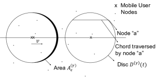
Figure 3: The disc around the mobile user with area $A^{(\gamma)}_{\epsilon}$ and the chord along which the node moves.

Since the mobile moves at constant velocity, the distribution of the service times can be derived from the distribution of the chord lengths. Without loss of generality suppose the mobile moves along the x-axis, then clearly the $y$ coordinate of a typical node entering the disc, $Y^{(\gamma)}$ is uniform on [$-r_{\gamma},r_{\gamma}$]. The random variable $W^{(\gamma)}$ representing the service time is then given by:

$$W^{(\gamma)}=\frac{2\sqrt{r_{\gamma}^{2}-(Y^{(\gamma)})^{2}}}{v}.$$

The density of $W^{(\gamma)}$ is (5), and the mean service time is $E[W^{(\gamma)}]=\frac{\pi r_{\gamma}}{2v}$.

Thus, the process $(K^{(\gamma)}(t),t\geq 0)$ capturing the number of nodes in the moving disc follows the dynamics of the number of customers in an $M/GI/\infty$ queue with arrival rate $\lambda^{({\gamma})}=2r_{\gamma}v\lambda$ and general independent service times following the distribution of $W^{(\gamma)}$. It follows that the stationary distribution for $K^{(\gamma)}(t)$ is Poisson with mean $\pi r_{\gamma}^{2}\lambda$ . ∎

Given the connection to an $M/GI/\infty$ queueing model, the SNR level crossing process is an alternating renewal process defined as follows:

Definition 2.

A process alternating between successive on and off intervals is an alternating renewal process if the sequences of on period $(B^{(\gamma)}_{n},n\geq 1)$ and off period $(I^{(\gamma)}_{n},n\geq 1)$ are independent sequences of i.i.d. non-negative random variables.

Theorem 2.

For all $\gamma>0$, the SNR level crossing process, $(C^{(\gamma)}(t),t\geq 0)$, is an alternating-renewal process. Further, its typical on period, $B^{(\gamma)}$, and off period, $I^{(\gamma)}$, are distributed as the busy and idle periods of an $M/GI/\infty$ queue with arrival rate $\lambda^{({\gamma})}=2r_{\gamma}v\lambda$ and i.i.d. service times with distribution given in (5). Thus, $I^{(\gamma)}\sim\exp(2\lambda vr_{\gamma})$ and the busy period distribution can be explicitly characterized as in  [12]. Also, in the stationary regime, the probability that the SNR level crossing process is “on” is $1-e^{-\lambda\pi r_{\gamma}^{2}}$.

Proof.

Let us consider the $M/GI/\infty$ queue defined in Theorem 1. The queue being empty implies that there are no nodes closer than distance $r_{\gamma}$ from the tagged user. Thus, an off period of the associated SNR level crossing process is equivalent to an idle period of the queue. Similarly, the busy period is equivalent to an on period.

Since the arrival process is Poisson, the inter arrival times are exponential with parameter $\lambda^{(\gamma)}=2\lambda vr_{\gamma}$. Because of the memoryless property, all the idle periods obey the same distribution.

Let $\hat{B}^{(\gamma)}$ denote a random variable representing the forward recurrence time associated with the on time defined as

$$\mathbb{P}(\hat{B}^{(\gamma)}>x)=\frac{1}{\mathbb{E}[B^{(\gamma)}]}\int_{x}^{\infty}\mathbb{P}(B^{(\gamma)}>z)dz.$$ (6)

Using the correspondence of the SNR on times with the busy period of the $M/GI/\infty$ queue considered, its distribution is same as that given in Theorem 12 in the Appendix with service time $S\sim W^{(\gamma)}$ and

$$\rho^{(\gamma)}=2r_{\gamma}v\lambda\mathbb{E}[W^{(\gamma)}]=\lambda\pi r_{\gamma}^{2}~{}\mbox{,}~{}~{}\nu^{(\gamma)}=1-e^{-\rho^{(\gamma)}}.$$ (7)

Also, the busy period $B^{(\gamma)}$ depends upon the arrivals and service times of customers arriving after the customer initiating the busy period which are independent of the past arrivals. Thus the busy period $B^{(\gamma)}$ and idle period $I^{(\gamma)}$ are independent. Hence, the SNR level crossing process form an alternating-renewal process.

The mean of the busy period of the queue is given by [12]:

$$\mathbb{E}[B^{({\gamma})}]=\frac{\nu^{({\gamma})}}{2\lambda vr_{\gamma}(1-\nu^{({\gamma})})}.$$ (8)

Thus, the probability that the SNR level crossing process is “on” is $1-e^{-\lambda\pi r_{\gamma}^{2}}$.

∎

It is easy to see that all path loss functions which are monotonic lead to an analogue of Theorem 2.

III-B Fluctuations of the SNR Process

The SNR process is pathwise continuous and has continuous derivatives except at a countable set of times corresponding to Voronoi cell edge crossings where the mobile sees a hand-off and where the first derivative of the SNR process is discontinuous.

Since the mobile is moving with a fixed velocity $v$, the intensity of the cell-edge crossings is given by $4v\sqrt{\lambda}/\pi$ [13], [14].

As the mobile traverses a particular cell, there is a time where it is the closest to the associated node. The SNR process has a local maximum at these times. Perhaps surprisingly such maxima may happen at the edge of the cell. Let us denote the point process of interior maxima by $\chi$. The (time) intensity of $\chi$ is given in the following theorem.

Theorem 3.

The intensity of the point process $\chi$ of the SNR maxima occurring in the interior of cells is $v\sqrt{\lambda}$.

Proof is given in Appendix A.

Thus, the fraction of SNR maxima that happen in the interior of the cell is given by $\pi/4$. In other words, $1-\frac{\pi}{4}$ of the SNR maxima seen by the mobile occur at the cell edges.

III-C Rare Events

In this subsection we consider certain rare events such as the occurrence of large SNR values. We show that the “rarity hence exponentiality” principle [10, 11] applies here. We also give the scales at which the inter-arrival time of high SNR is close to an exponential. As we shall see in Section VII, these asymptotic results can also be used for moderate values of SNR for the parameters typically found in wireless networks.

The following theorem gives a characterization of the asymptotic behavior of the distribution of the random variable $V^{(\gamma)}$ corresponding to the up-crossings as $\gamma\to\infty$ and as $\gamma\to 0$, which can be seen as “good” and “bad” events respectively.

Theorem 4.

For all $\gamma>0$, the up-crossings of the SNR level crossing process, $(T_{n}^{(\gamma)},n\geq 1),$ constitute a renewal process. Let $V^{(\gamma)}$ be the typical inter arrival for this process. Let $f(\gamma)=2\lambda vr_{\gamma}$, then

$$\lim_{\gamma\to\infty}f(\gamma)V^{(\gamma)}\xrightarrow{d}\exp(1).$$

Let $g(\gamma)=2\lambda vr_{\gamma}e^{-\lambda\pi r_{\gamma}^{2}}$ , then

$$\lim_{\gamma\to 0}g(\gamma)V^{(\gamma)}\xrightarrow{d}\exp(1).$$

Proof.

The proof is given in the Appendix.
Notice that as $\gamma\to\infty$, the radius of coverage $r_{\gamma}\to 0$ and vice versa. The scale $f(\gamma)^{-1}$ of the inter-event times of “good events” is sub-linear in $r_{\gamma}$ when $r_{\gamma}$ tends to 0, whereas the scale $g(\gamma)^{-1}$ for “bad events” is exponential in the variable $r_{\gamma}^{2}$ when $r_{\gamma}$ tends to infinity. Thus, the good events happen in a sense more often than the bad events.

For bad events, as $r_{\gamma}$ tends to $\infty$, a disc of radius $r_{\gamma}$ should be empty whose probability is given by $e^{-\lambda\pi r_{\gamma}^{2}}$. Conversely, for good events, as $r_{\gamma}$ tends to 0, there should at least be a node in the disc of radius $r_{\gamma}$, an event whose probability is given by $1-e^{-\lambda\pi r_{\gamma}^{2}}$. Thus, the difference in scale is due to the fact that the probability of occurrence of a bad event goes to zero with $r_{\gamma}$ tending to infinity, faster than the probability of occurrence of good event with $r_{\gamma}$ tending to 0. ∎

IV Sharing Number Process

In contrast to the SNR or the Shannon rate process, which take their values in the continuum, the sharing number process takes a discrete set of values and is piece-wise constant. We shall start by evaluating the frequency of discontinuities and then introduce an upper-bound process to be used in the sequel. We conclude this section with a study of rare events.

IV-A Discontinuities

In the sequel, we will use the following simplified notion of a Johnson-Mehl cell, see [13].

Definition 3.

Consider $\Phi=\{X_{i}\}$ the Poisson point process of nodes on $\mathbb{R}^{2}$. For any threshold $\gamma$, the Johnson–Mehl cell $J^{(\gamma)}(X_{i})$ associated with $X_{i}$ is the intersection of the Voronoi cell of $X_{i}$ w.r.t. $\Phi$ with a disc of radius $r_{\gamma}$ centered at $X_{i}$, see Fig.4.

Thus for a fixed threshold $\gamma$, the mobile user is covered/served at time $t$ if and only if it is within the Johnson–Mehl cell of its associated node $X(t)$ for the radius $r_{\gamma}$. We recall that:

Definition 4.

The process $(N^{(\gamma)}(t),t\geq 0)$ is defined as the number of static users present in the Johnson-Mehl cell $J^{(\gamma)}(X(t))$ if the mobile is in $J^{(\gamma)}(X(t))$ and 0 otherwise.

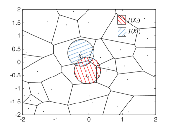
Figure 4: Johnson-Mehl cells.

The process $(N^{(\gamma)}(t),t\geq 0)$ is an ${\mathbb{N}}$-valued piece-wise constant process, with jumps at certain Johnson–Mehl cell edge crossings as illustrated in Figure 5. The value it assumes upon entering a cell is a conditionally Poisson random variable with a parameter that depends on the area of the cell in question. The following theorem provides an upper bound for the jump intensity:

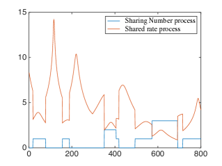
Figure 5: Trace of the Sharing number and Shared rate processes

Theorem 5.

An upper bound for the intensity of discontinuities of the sharing number process is the intensity of the Johnson-Mehl cell edge crossings, which is given by:

$$\frac{4v\sqrt{\lambda}}{\pi}(\mbox{erf}(\sqrt{\lambda\pi}r_{\gamma}-2\sqrt{\lambda}r_{\gamma}e^{-\lambda\pi r_{\gamma}^{2}}).$$

Proof.

The intensity of cell edge crossings in a Johnson-Mehl tessellation is given in [15]. Not all the cell edge crossings lead to jumps as the number of static users can be the same across two adjacent Johnson-Mehl cells, thus the given intensity is an upper bound. ∎

Given that the value of $N^{(\gamma)}(t)$ is a non-zero constant, the time of constancy is defined as the typical amount of time it remains at that same constant. This time of constancy is lower bounded by the distribution of the chord length of the motion line’s intersection with a typical Johnson–Mehl cell [15]. It is a lower bound only since the number of static users can be the same across two adjacent Johnson-Mehl cells.

IV-B Upper Bound for the Sharing Number Process

Note that the two underlying processes that are used to define the shared rate process, namely the sharing number process $(N^{(\gamma)}(t),t\geq 0)$ and the SNR process $(\mbox{SNR}(t),t\geq 0)$, are not independent as easily seen in the case where $\gamma=0$. For example, assume that the mobile user experiences a low SNR, i.e., it is far from its associated node, Then the area of the Voronoi cell is likely to be large. This in turn implies that the mobile is more likely to share its node with a large number of users.

Fortunately, the sharing number process admits a simple upper bound which is independent of the SNR process. This upper bound is defined as follows:

Definition 5.

Let $D(x,r_{\gamma})$ denote a disc of radius $r_{\gamma}$ centered at location $x$. Let $\hat{N}^{(\gamma)}(t),t\geq 0,$ be the number of static users which are in the disc $D(X(t),r_{\gamma})$ if the mobile is in $J^{(\gamma)}(X(t))$, and 0 otherwise.

The stochastic process $(\hat{N}^{(\gamma)}(t),t\geq 0)$ enjoys most of the structural properties of $({N^{(\gamma)}}(t),t\geq 0)$; in particular, it is piece-wise constant and one can derive natural bounds on the intensity of its jumps. In addition and more importantly:

• For all $t\geq 0$, $\mathbb{P(}\hat{N}^{(\gamma)}(t)\geq N^{(\gamma)}(t))=1$, i.e., $\hat{N}^{(\gamma)}(t)$ is an upper bound for the sharing number; this bound is tight in the regime where the area of the typical Voronoi cell ($\frac{1}{\lambda})$ is large compared to the area of the disc of radius $r_{\gamma}$;

• When the mobile user is covered, the sharing number $\hat{N}^{(\gamma)}(t)$ is Poisson with parameter $\xi\pi r_{\gamma}^{2}$;

• The stochastic processes $(\hat{N}^{(\gamma)}(t),t\geq 0)$ and $(\mbox{SNR}(t),t\geq 0)$ are independent.

V Shared Rate process

We recall that the shared rate is

$$S^{(\gamma)}(t)=R^{(\gamma)}(t)F^{(\gamma)}(t)=R^{(\gamma)}(t)\frac{1}{N^{(\gamma)}(t)+1},$$ (9)

with $R^{(\gamma)}(t)$ the Shannon rate defined in (2) and $F^{(\gamma)}(t)$ the sharing factor at time $t$. A realization of this process is illustrated in Figure 5. In the sequel, we use our upper bound process on $N^{(\gamma)}(t)$ to obtain a lower bound on the shared rate:

$$\hat{S}^{(\gamma)}(t)=R^{(\gamma)}(t)\hat{F}^{(\gamma)}(t)=R^{(\gamma)}(t)\frac{1}{\hat{N}^{(\gamma)}(t)+1},$$ (10)

which is now a product of two independent random variables.

V-A Shared Rate Variability

The shared rate process is smooth for Lebesgue almost every $t$, with a countable set of discontinuities and a countable set of points of discontinuities of its first derivative. It is equal to zero when the mobile is not covered. The point process of discontinuities is upper bounded by the Johnson-Mehl cell edge crossings (see Theorem 5). The point process of its local maxima where the derivative is zero is the same as that of the SNR process as given in Theorem 3.

As can be seen from (10), the variability in the mobile user’s shared rate is driven by two processes: the Shannon rate and the sharing factor process. It is of interest to understand their relative contributions. To answer this question, let us consider the variance of $\hat{S}^{(\gamma)}$ which can be written using the conditional variance formula as:

$$\mbox{var}(\hat{S}^{(\gamma)})=\mbox{var}(R^{(\gamma)})\mathbb{E}[\hat{F}^{(\gamma)}]^{2}+\mbox{var}(\hat{F}^{(\gamma)})(\mathbb{E}[(R^{(\gamma)})^{2}]).$$ (11)

Note that if the density of users increases, the variance of the shared factor decreases whereas the variance of the Shannon rate remains constant. Thus, the variance of the shared rate varies approximately linearly with a slope equal to the second moment of the Shannon rate. By contrast if the density of nodes increases, the variance of both the sharing factor and Shannon rate vary making their relative contributions more complex.

Let us see empirically what are the contributions of the user and node density to the variability of shared rate. For a given node density $\lambda=25/\pi$ and radius of coverage $r_{\gamma}=500m$, by increasing the density of static users, the variance of the shared rate decreases linearly with the variance of the sharing factor. Table II gives numerical values evaluated by simulations. For a given static user density $\xi=50$ and radius of coverage of $200m$, by increasing the density of nodes the variance of both the sharing factor and Shannon rate varies. Table III gives numerical values evaluated by simulations.

$\xi$	var($S^{(\gamma)}$)	var($\hat{F}^{(\gamma)}$)
5	0.6527	0.0303
25	0.0674	0.0028
50	0.012	0.0016
75	0.0047	0.0006
100	0.0023	0.0001

TABLE II: Variance values when increasing user density.

$\lambda$	var($S^{(\gamma)}$)	var($\hat{F}^{(\gamma)}$)	var($R^{(\gamma)}$)
5	0.0438	0.0049	0.3325
25	5.1292	0.0576	03.3944
50	0.6351	0.0642	0.9607
75	01.2626	0.0723	0.6926
100	0.9682	0.0756	0.2252

TABLE III: Variance values when increasing node density.

These results confirm that whereas the impact of increasing the other users density on mobile user’s shared rate variance is clear, the result of increasing the density of nodes is more subtle.

V-B Rare Events

Since the mobile user’s shared rate depends on two components it is of interest to understand their relative contributions towards the events of high/low shared rate. The proofs of the following theorems are given in Appendix.

Theorem 6.

The likelihood of the rare events associated with high shared rates is the same (up to logarithmic equivalence) as that for the high SNR in the sense that

$$\lim_{s\to\infty}-\frac{1}{s}\log\left(\mathbb{P}(S^{(\gamma)}>s)\right)$$

$$= \lim_{s\to\infty}-\frac{1}{s}\log\left(\mathbb{P}(\log(1+{\mathrm{SNR}})>s)\right)=\frac{2}{\beta}.$$

Notice that as a direct corollary of the last theorem,

$$\lim_{s\to\infty}-\frac{1}{s}\log\left(\mathbb{P}(S^{(\gamma)}>s)\right)$$

$$= \lim_{s\to\infty}-\frac{1}{s}\log\left(\mathbb{P}(S^{(\gamma)}>s|N^{(\gamma)}=0)\right)$$

$$= \lim_{s\to\infty}-\frac{1}{s}\log\left(\mathbb{P}(S^{(\gamma)}>s,N^{(\gamma)}=0)\right)=\frac{2}{\beta}.$$

For the rare events associated with a low shared rate, we will consider the lower bound process $(\hat{S}^{(\gamma)}(t),t\geq 0)$:

Theorem 7.

The rare events of low shared rates are predominantly the same as the rare events of high sharing number given that the mobile is at the covering cell edge, in the sense that for some sequence $\{s_{n}\}$ such that $s_{n}\log(1+Kr_{\gamma}^{-\beta})\in\mathbb{Z}~{}\forall n$ and $\lim_{n\to\infty}s_{n}\to\infty$:

$$\lim_{n\to\infty}-\frac{1}{s_{n}\log(s_{n})}\log\left(\mathbb{P}\left(\hat{S}^{(\gamma)}<\frac{1}{s}_{n}\right)\right)$$ (12)

$$= \lim_{n\to\infty}-\frac{1}{s_{n}\log(s_{n})}\log\left(\mathbb{P}\left(\frac{\log(1+Kr_{\gamma}^{-\beta})}{\hat{N}^{(\gamma)}+1}<\frac{1}{s}_{n}\right)\right)$$

$$= \log(1+Kr_{\gamma}^{-\beta}).$$

Theorem 8.

Conditioned on a very good or bad shared rate, the relative contribution of the mobile user’s location and the network congestion is as follows:

$$\lim_{s\to\infty}\mathbb{P}(R^{(\gamma)}>s,N^{(\gamma)}=0|S^{(\gamma)}>s)=1.$$ (13)

$$\mathbb{P}(N^{(\gamma)}>as\log(1+\gamma)-1|0<S^{(\gamma)}<1/s)=1.$$ (14)

Conditioned on a very high shared rate, the mobile user has to be close to the associated node with no other static users sharing its resources. On the contrary, conditioned on the mobile being served and experiencing a very low shared rate, it has to share its associated node with number of users that is inversely proportional to the desired shared rate.

From the previous theorem, we know that high shared rates are predominantly the same as the event where the SNR is high and the sharing number is zero. Thus, for a given threshold $\delta$ for the shared rate process, we can study the asymptotic behavior of the distribution of the inter arrival time of shared rate up-crossings as $\delta\to\infty$.

Corollary 1.

Let $\hat{Z_{\delta}}$ denote the inter arrival time for the good events of the lower bound process $(\hat{S}^{(\gamma)}(t),t\geq 0)$. Then

$$\lim_{\delta\to\infty}f(r_{\delta})e^{-\xi\pi r_{\gamma}^{2}}\hat{Z_{\delta}}\to\exp(1),$$

where $f(r_{\delta})=2\lambda vr_{\delta}.$

Proof.

The result follows from the fact that $\hat{Z_{\delta}}=\sum_{i=1}^{X}V^{r_{\delta}}$, where $X$ is geometric random variable with parameter $e^{-\xi\pi r_{\gamma}^{2}}$ and $V^{(r_{\delta})}$ the typical interval time of the renewal process of up-crossings associated with the SNR process of threshold $\delta$. ∎

VI Simulation and Validation

In this section we evaluate when our mathematical model and associated asymptotic results are valid in more realistic settings. We use simulation to study the temporal variations of the SNR process experienced by a mobile user under various scenarios which are are not captured by our analytical framework. The model is challenged in various complementary ways: e.g., by adding fading and accounting for interference from other base stations. In each case the objective is to determine for what parameter values of the additional feature our simplified mathematical model is still approximately valid, providing robust engineering rules of thumb to predict what mobile users will see.

In particular, we will answer the following questions:

• How quickly do the SNR level up crossings converge to exponential asymptotics as a function of the associated thresholds?

• Are the results obtained robust to the addition of fast fading?

• Are there regimes where the temporal characteristics of the SNR process are a good proxy for the SINR process, e.g., high path loss?

We begin by introducing our simulation methodology and the default parameters used throughout this section.

VI-A Simulation Methodology

We consider a user moving on a straight line (road) at a fixed velocity of 16 m/s. The base stations are randomly placed according to a Poisson point process with intensity $\lambda$ such that the mean coverage area per base station is that of a disc with radius 200m. Unless otherwise specified, we consider the path loss function given by Eq. (1) with exponent $\beta=4$ and assume that all base stations transmit with equal power of $p=2\mbox{W}$. The signal strength received by the mobile user is recomputed every $10^{-2}$ seconds.

We calibrate the thermal noise power to the cell-edge user. Let $D$ be a random variable denoting the distance from a typical user to the closest base station. Define $d_{{edge}}$ by the relation $P(D\leq d_{{edge}})=0.9$. Since in our simulation setting $P(D\leq d)=1-\exp(\lambda\pi d^{2})$, we have $d_{{edge}}=\sqrt{\frac{-\ln(0.1)}{\pi\lambda}}$. If we fix the desired SNR at the cell edge to be $\mbox{SNR}_{{edge}}$ this then determines the noise power to be $w=\frac{pd_{{edge}}^{-\beta}}{\mbox{SNR}_{{edge}}}$.

In the sequel we evaluate how quickly the convergence to exponential studied in Theorem 4 arises. To that end we compare the renormalized distributions obtained via simulation to the reference exponential distribution with parameter 1, using the Kolmogorov-Smirnov (K-S) test. The K-S test finds the greatest discrepancy between the observed and expected cumulative frequencies– called the “D-statistic”. This is compared against the critical D-statistic for that sample size with 5% significance level. If the calculated D-statistic is less than the critical one, we conclude that the distribution is of the expected form, see e.g. [16].

VI-B Convergence of Level-crossing Asymptotics

Theorem 4 indicates that as the SNR threshold $\gamma$ in dB increases, the rescaled distribution for up-crossings of the SNR process becomes exponential. The question is how large $\gamma$ needs to be for this result to hold. To that end we simulated the level crossing process for various $\gamma$ and computed the D-statistic mentioned above. The empirical CDF for up-crossing inter-arrivals rescaled by $f(r_{\gamma})$ as introduced in the theorem can be seen in e.g., Fig. 6. As expected we found that as the threshold increases, the distribution becomes exponential, and for a threshold value of $\gamma=50$ or more, it is exponential with unit mean.

In practice SNR of 50 dB is not realistic for wireless users. However, as seen from Figure 6, for moderate values of $\gamma$ such as $0.1,1$, the up-crossing inter-arrivals can be approximated by an exponential with parameter $1/f(r_{\gamma})$. For $\gamma=1$, the empirical mean for the inter-arrival time for up-crossings is $72.4s$ and the asymptotic approximated mean i.e., $f(r_{\gamma})^{-1}$ is $63.07s$.

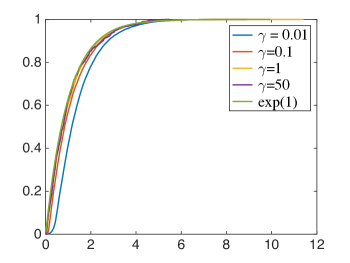
Figure 6: CDF of interarrival of up-crossings for various thresholds.

VI-C Robustness of Level-crossing Asymptotics to Fading

Next we study the effect that channel fading might have on the level-crossing asymptotics. We consider channels with Rayleigh fading with unit mean, so that the SNR experienced by the tagged mobile user at a distance $d$ from the base station is given by $Hpd^{-\beta}/w$, where $H$ is a fading random variable which is exponential with unit mean. The coherence time is set to $t_{c}=0.423/f_{d}$, where $f_{d}$ is the Doppler shift given by $f_{d}=\frac{v}{c}f_{o}$ where $v$ is the vehicle velocity, $c$ is the speed of lights and $f_{o}=900\mbox{MHz}$ is the operating frequency. This gives a coherence time $t_{c}=0.007s$. Thus, fading (power) changes every 0.007 seconds. The SNR process with fading is illustrated in Fig. 7.

Clearly when we incorporate channel fading in the SNR process, even when one fixes a high SNR threshold, the level-crossing process has additional fluctuations before it goes down again for some time, see Fig. 7. Thus to exhibit the on-off structure and asymptotics we consider a modified process defined as follows. After the first up-crossing, we suppress all subsequent up crossings (if any) for an appropriate time period, and then look for the next up-crossing taking place after this time. We take a time period for the suppression of up-crossings equal to twice the expected on time of $2E[B^{(r_{\gamma})}]$  [12].

In order to vary the variance while keeping the mean of the fading at one, we now consider fading which is a mixture of exponentials. For this process, we would expect that for fading with mean one, if variance is small, the appropriately rescaled inter-arrival distribution for up-crossings which are not suppressed would once again asymptotically become exponential with parameter 1. In other words we expect geometric variations associated with base station locations to dominate channel variations. Whereas, if the fading variance is high, one might expect the SNR threshold required to obtain convergence to an exponentiality to increase. Fig. 8 plots such thresholds as a function of the fading variance. As can be seen for fading variances exceeding $8$, the channel variations dominate the geometric variations and thus up-crossing asymptotics differ from Theorem 4.

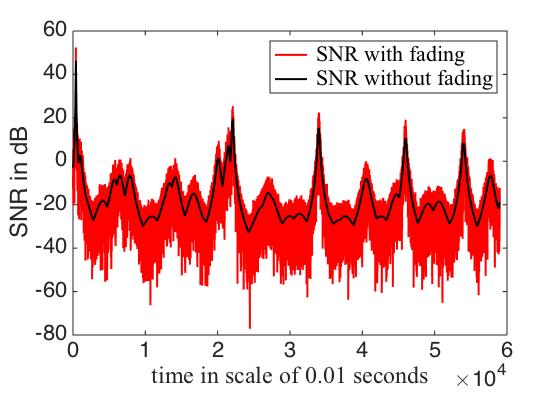
Figure 7: SNR process in presence of fading with mean 1.

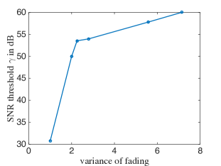
Figure 8: Threshold above which the inter-arrival of up-crossing converge to exponential with parameter 1 for different variance of fading.

VI-D Robustness of Level-crossing Asymptotics to Interference

So far we have focused on the SNR process. One might ask to what degree the Signal-to-Interference-plus-Noise Ratio (SINR) process, shares similar characteristics.

We first simulated the SINR process for a setting with a high path loss exponent of $\beta=4$ and found once again that the rescaled distribution for the up-crossing inter-arrivals converges to an exponential with parameter 1. The test requires a threshold $\gamma=31.7$dB. However, as seen above, this asymptotic is already useful for moderate values of $\gamma$. We then evaluated, for different path loss $\beta$, what threshold values were needed to obtain a similar convergence. As shown by Fig. 9, the threshold in question increases as $\beta$ decreases. Further we found that for $\beta<3.5$, we no longer have the desired convergence property. In summary, for high path-loss exponents $\beta=3.5-4$, the up-crossing asymptotics for the SNR and SINR processes are similar.

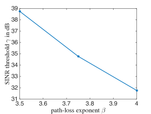
Figure 9: Threshold above which the inter-arrival of up-crossing converge to exponential with parameter 1 for different path loss exponent.

VII Applications

In this section we consider our models to evaluate application-level performance of mobiles in a shared wireless network. In particular we consider two very different wireless scenarios: (1) video streaming to mobiles sharing a cellular or Wifi network and (2) large file downloads using Wifi.

VII-A Stored Video Streaming to Mobile Users

Let us consider a scenario where mobile users are viewing stored videos which are streamed over a sequence of wireless downlinks. The users are distributed according to a Poisson point process of density $\xi$ and are moving independently of each other. Consider a policy where a mobile user is served by a node only if the SNR experienced is greater than a threshold $\gamma$. Thus, the nodes serve the mobile users within the radius of coverage $r_{\gamma}=(p/(\gamma w))^{1/\beta}$. A lower threshold $\gamma$ corresponds to a lower transmission rate (when served), a higher probability of coverage and sharing with a large number of other mobile users. Conversely a higher threshold implies higher transmission rate and sharing with fewer other mobile users. For simplicity we consider rebuffering as the primary metric for user’s video quality of experience [9].

The playback buffer state of the tagged mobile user moving at a fixed velocity $v$ on a straight line, can be modeled as a fluid queue. The arrival rate to which alternates between an average ergodic rate, $h(\gamma)=\mathbb{E}[R^{(\gamma)}|\mbox{SNR}>\gamma]$ and zero depending on whether the mobile is being served or not. Let $\eta$ denote the video playback rate in bits. Hence, as long as the buffer is non-empty, the fluid depletion rate of the queue is $\eta$. Re-buffering of the video is directly linked to the proportion of time the playback buffer is empty, which is given by $1-\rho(\gamma,\xi)$, where the load factor, $\rho(\gamma,\xi)$, [17] of the queue is:

$$\rho(\gamma,\xi)=\frac{\nu^{(\gamma)}h(\gamma)}{\eta}\mathbb{E}\bigg{[}\frac{1}{N_{p}^{(\gamma)}+1}\bigg{]}.$$ (15)

where $\nu^{(\gamma)}$ is the probability that the alternating renewal process associated with the arrival rate to the fluid queue is “on”.

The first natural question one can ask is whether there is a choice of $\gamma$ such that the fluid queue is unstable, thus ensuring no rebuffering in the long term. In other words, does there exist a $\gamma>0$ such that $\rho(\gamma,\xi)>1$? Given our policy and the metric for quality of experience, the network provider has liberty to choose a lower value of threshold,$\gamma$, as long as the typical mobile user in the long run experiences no rebuffering.

Now, for simplicity let us consider a constant rate $\kappa=a\log\left(1+\gamma\right)\mathbb{E}\bigg{[}\frac{1}{N_{p}^{(\gamma)}+1}\bigg{]}$ instead of the average ergodic rate. This constant bit rate is when the network does not rely on adaptive coding/decoding. For additional motivation for this scenario, see [9]. The load factor $\rho(\gamma,\xi)$ is given by

$$\begin{split}\rho(\gamma,\xi)=\frac{a\log(1+\gamma)\left(1-e^{\frac{-b}{\gamma^{2/\beta}}}\right)}{\eta}\mathbb{E}\bigg{[}\frac{1}{N_{p}^{(\gamma)}+1}\bigg{]},\end{split}$$ (16)

where $b=\lambda\pi\left(\frac{p}{w}\right)^{\frac{2}{\beta}}$ and $\mathbb{E}[1/(N_{p}^{(\gamma)}+1)]$ can be calculated by numerical integration as described in previous section.

It is easy to check that the function $\rho(\gamma,\xi)$ has a unique maximum $\gamma^{*}$ on $(0,\infty)$. A plot of (16) and the value of $\gamma^{*}$ are illustrated in Fig. 10. Notice that for these parameters, the value of $\gamma^{*}$ increases with $\xi$.

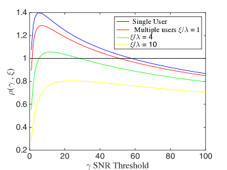
Figure 10: Load factor of the fluid queue for a single user (top curve) and for a positive density of users as a function of $\gamma$ (curves below the top curve). For the latter curves, the number of users per base station are $\xi/\lambda=1,4$ and 10 from top to bottom. Here $b=1$. All functions can be multiplied by an arbitrary positive constant when playing with $a$ and $\eta$.

For a given base station density $\lambda$ and density of users $\xi$, one can evaluate the SNR threshold value $\gamma^{*}$ for which the load factor $\rho$ is maximum. Fig.11 illustrates the level set curve of $\rho(\gamma^{*},\xi)=1$ for various values of $\lambda$ and $\xi$. In this setup, given the video consumption rate $\eta$, it is possible to answer questions like what is the minimum density of base stations required to serve a certain density of users such that the video streaming is uninterrupted for all the users.

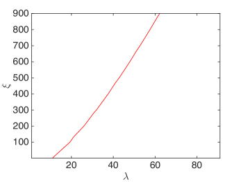
Figure 11: Level set curve of $\rho(\gamma^{*},\xi)=1$ for an arbitrary positive constants $a$ and $\eta$.

Remark 1.

In the case where there exists no threshold $\gamma$ for which the condition for no long term rebuffering is satisfied and $\kappa>\eta$, the fluid queue alternates between busy and idle period representing the periods when the video is un-interrupted or frozen, respectively. The distribution of the on periods $B^{(\gamma)}$ and that of the off periods $I^{(\gamma)}$ of of the $M/GI/\infty$ queue discussed in Section determine the distribution of the busy period $B_{f}$ and that of the idle period $I_{f}$ of the fluid queue. When denoting by $\kappa$ the constant input rate during on period and by $\eta$ the constant output rate when the queue is non-empty, the Laplace transform of $B_{f}$ is given by [18]

$$\mathcal{L}_{B_{f}}(s)=\mathcal{L}_{B^{(\gamma)}}(s\sigma+\lambda(\sigma-1)(1-\mathcal{L}_{B_{f}}(s))),$$ (17)

where $\sigma=\kappa/\eta>1$, and the idle period $I_{f}$ has an $\mbox{exp}(\lambda^{(\gamma)})$ distribution.

VII-B Wifi Offloading

WiFi offloading helps to improve spectrum efficiency and reduce cellular network congestion. One version of this scheme is to have mobile users opportunistically obtain data through WiFi rather than through the cellular network. Offloading traffic through WiFi has been shown to be an effective way to reduce the traffic on the cellular network. WiFi is faster and uses less energy to transmit data when there is a connection.

Let us consider a scenario where the mobile users download a large file from the service provider, relying on Wifi hotspots, distributed according to a Poisson point process of intensity $\lambda$, rather than on cellular base stations. The users are distributed according to a Poisson point process of density $\xi$ and are moving independently of each other. Assume that the Wifi hotspots have a fixed coverage area i.e., the mobile user connects to Wifi only if it is within a certain distance $r$ from the hotspot. Thus, higher the density of hotspots, $\lambda$, deployed by the provider the better the performance experienced by mobile users that rely only on them. We consider the time it takes to complete the download as the primary metric for user’s quality of experience.

Consider again the case without adaptive coding/decoding and the tagged mobile user moving on a straight line at constant velocity $v$.Then, the shared rate experienced by the mobile user is the constant $\kappa=a\log\left(1+\gamma\right)\mathbb{E}\bigg{[}\frac{1}{N_{p}^{(\gamma)}+1}\bigg{]}$ as defined above. In addition, the mobile user experiences an alternating on and off process, as characterized in Theorem 2.

Below, for the sake of mathematical simplicity, we assume that the file size $F$ is exponential with parameter $\delta$ and that the mobile user starts to download the file at the beginning of an on period. Let $T$ be a random variable denoting the time taken to download the file. Consider the event $J=\{F>\kappa B^{(\lambda)}\}$ and let

$$\alpha=\mathbb{P}(J)=\mathbb{P}(F>\kappa B^{(\lambda)})={\cal L}_{B^{(\lambda)}}(\delta\kappa).$$ (18)

Here and below, ${\cal L}_{X}(s)$ denotes the Laplace transform of the non-negative random variable $X$ at point $s$, and $B^{(\lambda)}$ is the random variable representing the length of a typical on interval seen by the mobile (see Theorem 2).

Now, define the non-negative random variables $X$ and $Y$ by their c.d.f.s

$$\mathbb{P}(X<x) = \frac{1}{\alpha}\int_{0}^{x}e^{-\delta\kappa z}f_{B^{(\lambda)}}(z)dz$$ (19)

$$\mathbb{P}(Y<y) = \frac{1}{1-\alpha}\int_{0}^{y}(1-e^{-\delta\kappa z})f_{B^{(\lambda)}}(z)dz.$$ (20)

Notice that

$${\cal L}_{X}(s) = \frac{1}{\alpha}{\cal L}_{B^{(\lambda)}}(s+\delta\kappa)$$ (21)

$${\cal L}_{Y}(s) = \frac{1}{1-\alpha}\left(1-{\cal L}_{B^{(\lambda)}}(s+\delta\kappa)\right).$$ (22)

The following representation of the Laplace transform of $T$ is an immediate corollary of the on-off structure:

Theorem 9.

Consider a network of Wifi hotspots distributed according to a Poisson point process of intensity $\lambda$ and radius of coverage $r$ shared by mobile users distributed independently by a Poisson point process of intensity $\xi$. Assuming that the tagged mobile user starts to download the file at the beginning of an on period, the Laplace transform of the time taken to download a file of size $F\sim\exp(\delta)$ is given by

$${\cal L}_{T}(s)=\frac{(1-\alpha){\cal L}_{Y}(s)}{1-\alpha{\cal L}_{X}(s)\frac{2\lambda vr}{2\lambda vr+s}}.$$ (23)

It is remarkable that the Laplace transform of $T$ admits a quite simple expression in terms of that of $B^{(\lambda)}$. Other and more general file distributions can be handled as well when using classical tools of Laplace transform theory. Note that this setting also leads to interesting optimization questions such as the optimal density of Wifi hotspots needed to be deployed for lower expected download times.

VIII Variants

In this section, we consider two generalizations of the previous framework: (1) we move from sharing with static users to sharing with mobile users and (2) we move from homogeneous to heterogeneous infrastructures

VIII-A Sharing the Network with Mobile Users

Until here we have considered a tagged mobile user sharing the network with static users. We now consider two scenarios: (1) that where the other users are mobile and are initially distributed according to a homogeneous Poisson point process and (2) that where they are mobile but restricted to a random road network, i.e., form a Cox process.

VIII-A1 Homogeneous Poisson case

Consider the case where other users sharing the network are initially located according to a homogeneous Poisson point process of intensity $\xi$, and subsequently exhibit arbitrary independent motion. This is a possible model for pedestrian motion. It follows from the displacement theorem for Poisson point processes [2] that the other users at any time instant will remain a Poisson point process of intensity $\xi$.

As considered before, the users are served only if they are at a distance less than $r_{\gamma}$ from the closest node. Consider a tagged mobile user moving at a fixed velocity along a straight line. Let us define the mobile sharing number process $(N_{p}^{(\gamma)}(t),t\geq 0)$ as the number of users sharing the node associated with the tagged user when it is served and zero otherwise. Thus, at any given time $t$, the tagged user shares its resources with a random number of users $N_{p}^{(\gamma)}(t)$ which is Poisson with a parameter depending on the area of the Johnson-Mehl cell.

For simplicity, we define the shared rate process $(S_{c}^{(\gamma)}(t),t\geq 0)$ as

$$S_{c}^{(\gamma)}(t)=\begin{cases}a\log\left(1+\gamma\right)\mathbb{E}\bigg{[}\frac{1}{N_{p}^{(\gamma)}+1}\bigg{]}&\text{if}~{}~{}L(t)\leq r_{\gamma},\\ 0~{}~{}&\text{otherwise}.\end{cases}$$ (24)

Since the distribution of the area of the Voronoi cell is unknown, we approximate $N_{p}^{(\gamma)}$ to be Poisson with parameter $\xi\mathbb{E}[\hat{J}^{(\gamma)}]$, where $\hat{J}^{(\gamma)}$ denotes the area of the Johnson-Mehl cell of radius $r_{\gamma}$, conditioned that the tagged user is within a distance $r_{\gamma}$ from the associated node, which introduces an additional bias. We can compute the expectation with the help of integral geometry as shown in Appendix F.

We found the value of the expectation using numerical integration and compared the mean number of users $\mathbb{E}[N_{p}^{(\gamma)}]=\xi\mathbb{E}[\hat{J}^{(\gamma)}]$ with the sample mean obtained from simulation for various parameters $\lambda,r_{\gamma}$. To validate the approximation of $N_{p}^{(\gamma)}$ by a Poisson random variable with parameter $\xi\mathbb{E}[\hat{J}^{(\gamma)}]$, we compared the value of $\mathbb{E}[1/(N_{p}^{(\gamma)}+1)]$ calculated using numerical integration with that of simulations. We found that the calculated value of the expectation is within the 95% confidence interval of the simulated mean.

VIII-A2 Cox process

Let us consider a population model where roads are distributed according to a Poisson line process of intensity $\lambda_{r}$ on $\mathbb{R}^{2}$ [19]. Then independently on each road, we consider users distributed according to a stationary Poisson point process of intensity $\lambda_{t}$. This is known as Cox process and we denote it by $\Phi_{u}$ [19]. This model can be used to represent a car motion in a road network.

For a line $L$ of the line process, let us denote the orthogonal projection of the origin $O$ on $L$ by $(\theta,r)$ in polar coordinates. For $\theta\in[0,\pi)$ and $r\in\mathbb{R}$, $(\theta,r)$ is unique. Thus, a Poisson line process with intensity $\lambda_{r}$ is the image of a Poisson point process with the same intensity on half-cylinder $[0,\pi)\times\mathbb{R}$.

Suppose all users on the roads are moving arbitrarily but independently from each other. Thus, at any instant the distribution of users on a given road remains Poisson. Consider a tagged user moving along a given road, then we have the following theorem by [20].

Theorem 10.

$\Phi_{u}$ is stationary, isotropic, with intensity $\pi\lambda_{r}\lambda_{t}$. From the point of view of the tagged user i.e., under the Palm distribution the point process is the union of three counting measures: (1) the atom at $O$, (2) an independent $\lambda_{t}$-Poisson point process on a line through $O$ with a uniform independent angle and (3) the stationary counting measure $\Phi_{u}$.

Following our previous framework, let us define an another sharing number process $(N_{d}^{(\gamma)}(t),t\geq 0)$ as the number of users sharing the node associated with the tagged user when it is served and zero otherwise.

Evaluation of the mean of $N_{d}^{(\gamma)}$. Suppose the tagged user is at the origin $O$. Let the associated node $X(t)$ be at a distance $x$ from the origin. Let $d(0,\theta)$ be a line through the origin with $\theta$ uniform from $[0,\pi)$. From the aforementioned theorem, the number of sharing users $N_{d}^{(\gamma)}$ can be split into two terms: $N_{s}$ denoting the number of sharing users from stationary $\Phi_{u}$ and $N_{l}$ denoting the number of sharing users on the line $d(0,\theta)$.

Given any convex body $Z$, $\mathbb{E}[N_{s}(Z)]$ is given by $\pi\lambda_{r}\lambda_{t}\mbox{area}(Z)$ [21]. Let $\hat{J}^{(\gamma)}$ denote the area as defined before. Thus,

$$\mathbb{E}[N_{s}]=\pi\lambda_{r}\lambda_{t}\mathbb{E}[\hat{J}^{(\gamma)}],$$

where, $\mathbb{E}[\hat{J}^{(\gamma)}]$ is evaluated using integral geometry (see Appendix F).

Now, let $l(0,\theta)$ denote the length of the line $d(0,\theta)$ in the area $\hat{J}^{(\gamma)}$. Then, $N_{l}$, the number of sharing users on the line $d(0,\theta)$, is Poisson with parameter $\lambda_{t}l(0,\theta)$. Thus, $\mathbb{E}[N_{l}]=\lambda_{t}\mathbb{E}[l(0,\theta)]$.

One can evaluate $\mathbb{E}[l(0,\theta)]$ using integral geometry (see Appendix G). We have,

$$\mathbb{E}[N_{d}^{(\gamma)}]=\mathbb{E}[N_{s}]+\mathbb{E}[N_{l}]=\pi\lambda_{r}\lambda_{t}\mathbb{E}[\hat{J}^{(\gamma)}]+\lambda_{t}\mathbb{E}[l(0,\theta)].$$ (25)

Thus, the mean number of users sharing the tagged user’s association node is larger when the users are distributed according to a Cox process than when the users are distributed according to a Poisson point process, assuming that both have the same mean spatial intensity.

VIII-B Mixture of Pedestrian and Road Network

Suppose now we have two types of users : drivers who stay on roads, and pedestrians which are unconstrained. If pedestrians are supposed to follow a Poisson point process, from their point of view, the number of sharing users corresponds to the sum of a stationary Poisson point process and a stationary Poisson line process. On the other hand, from a driver’s point of view, the number of sharing users corresponds to the same sum, but in addition with a Poisson point process on a road passing through the driver. Thus, the mean number of sharing users is always greater for drivers. Thus, pedestrians are likely to share its node with fewer users than drivers.

VIII-C Heterogeneous Networks

Let us consider a deployment of micro-base stations $\hat{\Phi}=\{\hat{X}_{1},\hat{X}_{2},..\}$ distributed according to some homogeneous Poisson process of intensity $\hat{\lambda}$ independent of the existing macro-base stations $\Phi=\{X_{1},X_{2},..\}$. Assume that all micro-BS transmit at a fixed power $\hat{p}$.

Let us consider a mobile user moving at a fixed velocity $v$ along a straight line. For a given SNR threshold $\gamma$, the mobile is served by a micro-base station if its distance from its closest micro-BS is less than $\hat{r}_{\gamma}=(\hat{p}/w\gamma)^{1/\beta}$. Otherwise it is served by a macro-base station provided its distance from the closest macro-BS is less than $r_{\gamma}$.

Note that the SNR level crossing process as previously defined is again an alternating renewal process which now depends on the heterogeneous resource deployment.

Theorem 11.

For heterogeneous networks with preferential association to micro base stations, the probability that the stationary SNR level crossing process seen by a tagged user is “on” is $1-e^{-\pi(\lambda r_{\gamma}^{2}+\hat{\lambda}\hat{r}_{\gamma}^{2})}$. Also, the mean time for which the process is “on” is given by

$$\frac{e^{\pi(\lambda r_{\gamma}^{2}+\hat{\lambda}\hat{r}_{\gamma}^{2})}-1}{2v(\lambda r_{\gamma}+\hat{\lambda}\hat{r}_{\gamma})}.$$ (26)

Proof.

In order to characterize the SNR level crossing process, we establish a connection to a Boolean model. Assume that the mobile user is moving with unit velocity. Let $B(X_{i},r_{\gamma})$ denote the closed ball of radius $r_{\gamma}$ centered at $X_{i}$ and $B(\hat{X}_{i},\hat{r}_{\gamma})$ a closed ball of radius $\hat{r}_{\gamma}$ centered at $\hat{X}_{i}$. The union of all these closed balls forms a Boolean model

$${\cal E}=\bigg{(}\cup_{X_{i}\in\Phi}B(X_{i},r_{\gamma})\bigg{)}\cup\bigg{(}\cup_{\hat{X}_{i}\in\hat{\Phi}}B(\hat{X}_{i},\hat{r}_{\gamma})\bigg{)}.$$ (27)

Now, assume that $\cal E$ is intersected by the directed line $\vec{l}$. Note that the Boolean model under consideration has independent convex grains and thus the intersection $\cal E$ $\cap$ $\vec{l}$ yields an alternating sequence of “on” and “off” periods which are independent. Let $B_{h}^{(\gamma)}$ and $I_{h}^{(\gamma)}$ be random variables denoting the length of a typical on on and off periods respectively.

The distribution of the length of off period $I_{h}^{(\gamma)}$ is easy to establish using the contact distribution functions and is exponential with parameter $\lambda^{*}$ [13]:

$$f_{I_{h}^{(\gamma)}}(l)=\lambda^{*}e^{\big{(}-\lambda^{*}l\big{)}},$$

where, $\lambda^{*}$ is $2(\lambda+\hat{\lambda})\mathbb{E}[R_{h}^{(\gamma)}]$. Here $R_{h}^{(\gamma)}$ is the random variable denoting the radius of the closed ball and is given by

$$R_{h}^{(\gamma)}=\begin{cases}&r_{\gamma}~{}\mbox{w.p.}~{}~{}\frac{\lambda}{\lambda+\hat{\lambda}}\\ &\hat{r}_{\gamma}~{}\mbox{w.p.}~{}~{}\frac{\hat{\lambda}}{\lambda+\hat{\lambda}}.\\ \end{cases}$$ (28)

Thus, the mean off period under the assumption of unit velocity is

$$\mathbb{E}[I_{h}^{(\gamma)}]=\frac{1}{\lambda^{*}}=\frac{1}{2(\lambda r_{\gamma}+\hat{\lambda}\hat{r}_{\gamma})}.$$

Now, in the stationary regime, the probability that the mobile user is either within a distance $\hat{r}_{\gamma}$ from a micro-BS or a distance $r_{\gamma}$ from a macro-BS i.e., it’s SNR level crossing process is “on”, is given by the volume fraction[13]:

$$c=1-e^{(-(\lambda+\hat{\lambda})\bar{V})},$$ (29)

where

$$\bar{V}=\mathbb{E}[v_{d}(\mbox{typical grain})]=\pi\mathbb{E}[(R_{h}^{(\gamma)})^{2}]=\frac{\pi(\lambda r_{\gamma}^{2}+\hat{\lambda}\hat{r}_{\gamma}^{2})}{\lambda+\hat{\lambda}}.$$ (30)

Thus, $c=1-e^{-\pi(\lambda r_{\gamma}^{2}+\hat{\lambda}\hat{r}_{\gamma}^{2})}.$ The probability evaluated above does not depend on the velocity of the mobile user and thus holds for any constant velocity $v$.

The mean on period $\mathbb{E}[B_{h}^{(\gamma)}]$ can be evaluated using the following relation

$$c=\frac{\mathbb{E}[B_{h}^{(\gamma)}]}{\mathbb{E}[B_{h}^{(\gamma)}]+\mathbb{E}[I_{h}^{(\gamma)}]},$$

which results in

$$\mathbb{E}[B_{h}^{(\gamma)}]=\frac{e^{\pi(\lambda r_{\gamma}^{2}+\hat{\lambda}\hat{r}_{\gamma}^{2})}-1}{2(\lambda r_{\gamma}+\hat{\lambda}\hat{r}_{\gamma})}.$$

Since, the mobile user is moving with a fixed velocity $v$, the mean time for which the mobile user is “on” is given by $\frac{\mathbb{E}[B_{h}^{(\gamma)}]}{v}.$

∎

These results provide an analytical characterization of the impact of heterogeneous densification on the mobile user’s temporal performance. Let us now compare the performance improvement seen by the mobile user in a heterogeneous network as compared to that of a homogeneous network. The graphs in Fig. 12 and Fig. 13 illustrate the difference in the expected on-times and volume fraction of the networks respectively.

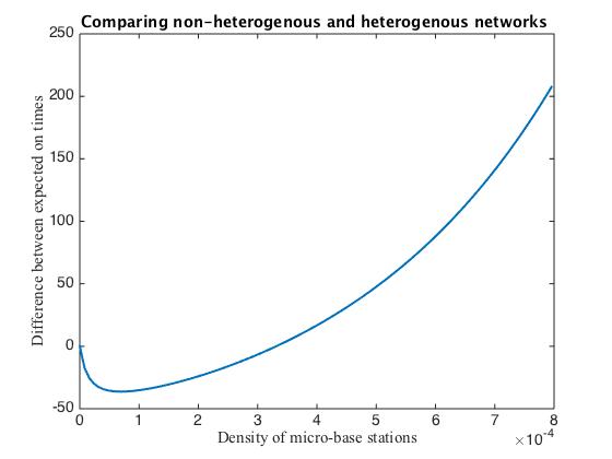
Figure 12: Comparing mean-on time for heterogeneous and homogeneous networks.

Figure 13: Comparing volume fraction for heterogeneous and homogeneous networks.

Notice that as micro-base stations are added, the expected on time decreases and later increases. The initial decrease is due to the inclusion of many relatively small length on-times resulting from the micro-base stations in the voids of the homogeneous network. However, the volume fraction increases monotonically with the addition of micro-base stations.

VIII-D Stored Video Streaming in Heterogeneous Networks

Consider a scenario as discussed before where mobile users are viewing a video being streamed over a sequence of wireless downlinks, but now in heterogeneous network with micro and macro BS. In this setting once again we consider a fluid queue representing the tagged mobile user’s playback buffer state similar to previous section and ask whether there is a choice of $\gamma$ such that the fluid queue is unstable, i.e., ensures no rebuffering in the long term. Let

$$\rho(\gamma,\xi)=\frac{a\log(1+\gamma)\mathbb{P}(\mbox{on})}{\eta}\left(\mathbb{E}\bigg{[}\frac{1}{N_{p}^{(\gamma)}+1}|\mbox{on}\bigg{]}\right).$$ (31)

Assuming our approximation is valid, we need to find $E[\frac{1}{N_{p}^{(\gamma)}+1}]$ in the case of heterogeneous network. Let events $G$ and $H$ be that the tagged user is served by micro BS and macro BS respectively.

$$\mathbb{E}\big{[}\frac{1}{N_{p}^{(\gamma)}+1}|\mbox{on}\big{]}=\frac{\bigg{(}\mathbb{E}\big{[}\frac{1}{N_{p}^{(\gamma)}+1}|G\big{]}\mathbb{P}(G)+\mathbb{E}\big{[}\frac{1}{N_{p}^{(\gamma)}+1}|H\big{]}\mathbb{P}(H)\bigg{)}}{\mathbb{P}(\mbox{on})}.$$ (32)

Since, the micro and macro base stations are distributed independently, the mobile user experiences two independent alternating renewal processes. Thus, in stationary regime, the probability that mobile is served by macro BS is the product of the probabilities that mobile is “on” period of alternating renewal process of macro BS and in “off” period of that of micro BS.

$$\mathbb{P}(G)=1-e^{-\hat{\lambda}\pi\hat{r}_{\gamma}^{2}},$$

$$\mathbb{P}(H)=e^{-\hat{\lambda}\pi\hat{r}_{\gamma}^{2}}(1-e^{-\lambda\pi r_{\gamma}^{2}}).$$

Let $\hat{J}_{1}^{(\gamma)}$ and $\hat{J}_{2}^{(\gamma)}$ denote the area similar to that of what we considered before. Given the mobile is served by macro BS, we need to consider the users which are within the area $\hat{J}_{1}^{(\gamma)}$ excluding the area covered by micro BS in this area. The area covered by the micro BS in $\hat{J}_{1}^{(\gamma)}$ is approximated to be $\nu^{(\hat{r}_{\gamma})}\times\mathbb{E}[\hat{J}_{1}^{\gamma}]$, where $\nu^{(\hat{r}_{\gamma})}$ is the volume fraction associated with micro-BS as given by (7). Then

$$\mathbb{E}\big{[}\frac{1}{N_{p}^{(\gamma)}+1}|G\big{]}=\frac{1-e^{\xi\mathbb{E}[\hat{J}_{2}^{(\gamma)}]}}{\xi\mathbb{E}[\hat{J}_{2}^{(\gamma)}]},$$

$$\mathbb{E}\big{[}\frac{1}{N_{p}^{(\gamma)}+1}|H\big{]}=\frac{1-e^{\xi\mathbb{E}[\hat{J}_{1}^{(\gamma)}](\hat{\lambda}\pi\hat{r}_{\gamma}^{2})}}{\xi\mathbb{E}[\hat{J}_{1}^{(\gamma)}](\hat{\lambda}\pi\hat{r}_{\gamma}^{2})}.$$

For a given density of macro-BS $\lambda$, the density of micro-BS $\hat{\lambda}$ and the density of users $\xi$, we can evaluate the SNR value $\gamma^{*}$ for which the load factor $\rho(\gamma,\xi)$ given in (31) is maximum. Fig.14 illustrates the optimal SNR value ($\gamma^{*}$) with varying density of micro BS $\hat{\lambda}$. Notice that the optimal gamma value initially decreases with the density of micro-BS.

Since in our setting the micro BS have smaller transmission power, for a given threshold $\gamma$, the radius of coverage for micro BS is smaller than that of the macro BS .i.e., $\hat{r_{\gamma}}<r_{\gamma}$. Since the micro-BS are given higher preference, with an increase in their density, the optimal threshold decreases in order to increase their coverage. Also, the cost incurred by increasing coverage of macro-BS is compensated by the increased density and coverage of micro-BS till a certain density.

Figure 14: $\gamma^{*}$ with increase in micro- BS density for a certain fixed density of macro-BS for an arbitrary positive constants $a$ and $\eta$ in heterogeneous case.

Fig.15 illustrates the level set curve of $\rho(\gamma^{*},\xi)=1$ for various values of $\hat{\lambda}$ and $\xi$ for a given density of macro-BS $\lambda$. Given this setup, it is possible to answer questions like what is the minimum density of micro-base stations that needs to be deployed by the operator to serve a certain density of users, given the density of macro-BS $\lambda$ such that the video streaming is uninterrupted for all the users. Thus, operators can learn the cost incurred to serve a higher density of users by deploying micro-BS and in case the cost incurred is higher, operator might be interested in other technologies.

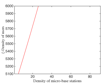
Figure 15: Level set curve of $\rho(\gamma^{*},\xi)=1$ for an arbitrary positive constants $a$ and $\eta$ in heterogeneous case.

Remark 2.

In heterogeneous networks, the interference from macro-BS to micro-Bs is of major concern. One can introduce blanking, to reduce the effect of such interference i.e., assume that with certain probability $f$ micro-BS transmit and with probability $1-f$ macro BS transmit.

Also, by considering heterogeneous networks with cellular BS and Wi-Fi hotspots, there is no such problem of interference since both cellular BS and Wifi hotspots operate at different frequencies.

IX Conclusion

As explained in the introduction, the analysis of temporal variations of the shared rate experienced by a mobile user requires the characterization of both the functional distribution of a continuous parameter stochastic process (rate process) constructed on a random spatial structure (e.g. the Poisson Voronoi tessellation) and of another stochastic process (sharing number process) constructed on a random distribution of static users. This paper addressed the simplest question of this type by focusing on the underlying SNR process and the sharing number process in the absence of fading. This allowed us to derive an exact representation of the level crossings of the stochastic process of interest as an alternating renewal process with a full characterization of the involved distributions and of the asymptotic behavior of rare events. The simplicity and the closed form nature of this mathematical picture are probably the most important observations of the paper. We also showed by simulation that this very simple model provides a good representation of the salient characteristics which happen for more complex systems, like e.g. those with fading when the fading variance is small enough, or those based on SINR rather than SNR when the path loss exponent is large enough. This model is hence of potential practical use as is, in addition to being a first glimpse at a set of new research questions. The most challenging questions on the mathematical side are probably (1) the understanding of the tension between the randomness coming from geometry (studied in the present paper), from sharing the network with other users (also studied in the present paper) and that coming from propagation (only studied by simulation here): it would be nice to analytically quantify when one dominates the other. (2) the extension of the analysis to SINR processes, which are our long term aim and will require significantly more sophisticated mathematical tools (e.g. based on functional distributions of shot noise fields), than those used so far. On the practical side, the main future challenges are linked to the initial motivations of this work, namely in the prediction and optimization of the user quality of experience. Many scenarios refining those studied can be considered. For instance, the stationary analysis of the fluid queue representing video streaming should be completed by a transient analysis and by a discrete time analysis. This alone opens an interesting and apparently unexplored connection between stochastic geometry and queuing theory with direct implications to wireless quality of experience.

X Acknowledgments

This work is supported in part by the National Science Foundation under Grant No. NSF-CCF-1218338, NSF Grant CNS-1343383 and an award from the Simons Foundation (No.197982), all to the University of Texas at Austin.

Appendix

X-A Proof of Theorem 3

The SNR process is closely related to the process tracking the distance of the mobile user to the closest node (see Eq. (1)). Let us consider the projection $z$ of the mobile user’s closest node $Z$ onto the straight line. Then, $z$ is a point of $\chi$ if $z$ lies within the Voronoi cell of $Z$. Thus, the point process can be characterized by the fact that given a node at a height $h$ from the straight line, the closed ball $B_{h}(z)$ of radius $h$ centered at the projection point is empty of nodes. Consider a rectangle of unit length and height $2x$ such that the straight line passes through the center. Thus, from Mecke’s formula [17], the intensity of the point process $\chi$ is

$$\begin{split}\mu_{\chi}&=v\lim_{x\to\infty}\lambda 2x\bigg{(}\int_{-x}^{x}e^{-\lambda\pi h^{2}}\frac{1}{2x}dh\bigg{)}\\ \\ &=v\lim_{x\to\infty}\sqrt{\lambda}\mbox{erf}(\sqrt{\lambda\pi}x)=v\sqrt{\lambda}.\end{split}$$ (33)

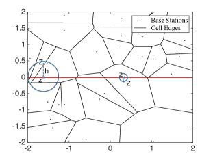
Figure 16: The disc $B_{z}(h)$ around the projection point $z$ in two scenarios: where $z$ belong to the Voronoi cell of nucleus $Z$ and where it doesn’t.

X-B Busy Period of the M/GI/$\infty$ Queue

Theorem 12.

(Makowski [12]) Consider an $M/GI/\infty$ queue with arrival rate $\lambda$ and generic service time $W$. Let $M$ denote an $\mathbb{N}$-valued random variable which is geometrically distributed according to

$$\mathbb{P}(M=l)=(1-\nu)(\nu)^{l-1},l=1,2,\ldots$$ (34)

with

$$\nu=1-e^{-\rho}~{}\mbox{and}~{}\rho=\lambda\mathbb{E}[W].$$ (35)

Consider the $\mathbb{R^{+}}$-valued random variable $U$ distributed according to

$$\mathbb{P}(U\leq u)=\frac{1}{\nu}(1-e^{-\rho\mathbb{P}[\hat{W}\leq u]}),u\geq 0,$$ (36)

where, $\hat{W}$ is the forward recurrence time associated with the generic service time $W$. Let $\{U_{n},n\geq 1\}$ be an i.i.d. sequence independent of the random variable $M$. Let $B$ denote a typical busy period. Then the forward recurrence time $\hat{B}$ associated with $B$ admits the following random sum representation:

$$\hat{B}=_{d}\sum_{i=1}^{M}U_{i},$$ (37)

where $=_{d}$ denotes equality in distribution.

X-C Proof of Theorem 4

$V^{({\gamma})}$ is the sum of the busy period $B^{({\gamma})}$ and the idle period $I^{({\gamma})}$ of the $M/GI/\infty$ queue. We know that the distribution of the idle period is exponential with parameter $2\lambda vr_{\gamma}$ and that the busy period $B^{({\gamma})}$ and idle period $I^{({\gamma})}$ are independent.

The Laplace transform of the random variable $V^{({\gamma})}$ scaled by $2\lambda vr_{\gamma}$ is given by

$$\Phi_{V^{(\gamma)}}(f(\gamma)s)=\Phi_{B^{({\gamma})}}(f(\gamma)s)\Phi_{I^{({\gamma})}}(f(\gamma)s),$$ (38)

where,

$$\Phi_{I^{({\gamma})}}(f(\gamma)s)=\frac{1}{1+s}.$$ (39)

So, asymptotically, as $r_{\gamma}$ goes to 0 , $\Phi_{I^{({\gamma})}}(f(\gamma)s)$ converges in distribution to an exponential random variable with unit mean.

Next, we need to prove that asymptotically, the busy period $B^{({\gamma})}$ scaled by $f(\gamma)$ goes to one. Let us consider the forward recurrence time of the busy period, $\hat{B}^{({\gamma})}$ which is defined in (6). Now from Theorem  2 we get,

$$\mathbb{E}[e^{-s\hat{B}^{({\gamma})}}]=\mathbb{E}[e^{-s\sum_{i=1}^{M^{({\gamma})}}U^{({\gamma})}_{i}}]=\frac{(1-\nu^{({\gamma})})\mathbb{E}[e^{-sU^{({\gamma})}}]}{1-\nu^{({\gamma})}\mathbb{E}[e^{-sU^{({\gamma})}}]}.$$

and it follows that

$$\mathbb{E}[e^{-sf(\gamma)\hat{B}^{({\gamma})}}]=\frac{(1-\nu^{({\gamma})})\mathbb{E}[e^{-sf(\gamma)U^{({\gamma})}}]}{1-\nu^{({\gamma})}\mathbb{E}[e^{-sf(\gamma)U^{({\gamma})}}]}.$$ (40)

Now,

$$\mathbb{E}[e^{-sf(\gamma)U^{({\gamma})}}]=\sum_{k=0}^{\infty}l_{k}(s,r_{\gamma}).$$ (41)

with

$$l_{k}(s,r_{\gamma})=\frac{(-1)^{k}(2\lambda vsr_{\gamma})^{k}\mathbb{E}[(U^{({\gamma})})^{k}]}{k!}.$$

Given that the support of service times $W^{({\gamma})}$ is $[0,2r_{\gamma}/v]$, it follows from (36) that the support of the random variable $U^{({\gamma})}$ is also $[0,2r_{\gamma}/v]$ and all its moments are bounded $\mathbb{E}[(U^{({\gamma})})^{k}]<(2r_{\gamma}/v)^{k}$. Thus, for all values of $s$, we get that $\lim_{r_{\gamma}\to 0}l_{k}(s,r_{\gamma})=0.$

For all $k=2,3..$ we have that

$$|l_{k}(s,r_{\gamma})|\leq\frac{(2\lambda vsr_{\gamma}^{2})^{k}}{k!}.$$

Therefore, for all values of $s$,$\lim_{r_{\gamma}\to 0}\sum_{k=2}^{\infty}l_{k}(s,r_{\gamma})=0.$

Thus, Eq (41) can be written as

$$\mathbb{E}[e^{-sf(\gamma)U^{({\gamma})}}]=1-s2\lambda r_{\gamma}v\mathbb{E}[U^{({\gamma})}]+o(r_{\gamma}),$$

Now, substituting into Eq (40) we have

$$\begin{split}&\mathbb{E}[e^{-sf(\gamma)\hat{B}^{({\gamma})}}]=\\ \\ &\frac{1-\nu^{({\gamma})}+2s\lambda vr_{\gamma}\mathbb{E}[U^{({\gamma})}](1-\nu^{({\gamma})})+o(r_{\gamma})}{1-\nu^{({\gamma})}+2\nu^{({\gamma})}s\lambda vr_{\gamma}\mathbb{E}[U^{({\gamma})}]+o(r_{\gamma})}.\end{split}$$ (42)

From which it follows that

$$\lim_{r_{\gamma}\to 0}\mathbb{E}[e^{-sf(\gamma)\hat{B}^{({\gamma})}}]=1.$$ (43)

From  [12] we have that

$$\mathbb{E}[e^{-sf(\gamma)B^{({\gamma})}}]=1-sf(\gamma)\mathbb{E}[B^{({\gamma})}]\mathbb{E}[e^{-sf(\gamma)\hat{B}^{({\gamma})}}],$$ (44)

and also

$$\mathbb{E}[B^{({\gamma})}]=\frac{\nu^{({\gamma})}}{2\lambda vr_{\gamma}(1-\nu^{({\gamma})})}.$$ (45)

Thus, we get

$$\mathbb{E}[e^{-sf(\gamma)B^{({\gamma})}}]=1-s\frac{1-e^{-\lambda\pi r_{\gamma}^{2}}}{e^{-\lambda\pi r_{\gamma}^{2}}}\mathbb{E}[e^{-sf(\gamma)\hat{B}^{({\gamma})}}].$$

Using the limit in (43), we get

$$\lim_{r_{\gamma}\to 0}\mathbb{E}[e^{-sf(\gamma)B^{({\gamma})}}]=1.$$ (46)

Thus, the distribution of the random variable $V^{({\gamma})}$ scaled by $f(\gamma)=2\lambda vr_{\gamma}$ converges in distribution to an exponential random variable with unit mean.

Now, consider a continuous function $g(\gamma)$ such that $\lim_{r_{\gamma}\to\infty}g(\gamma)=0$. The Laplace transform of the random variable $V^{({\gamma})}$ scaled by $g(\gamma)$ is given by

$$\Phi_{V^{({\gamma})}(s)}=\Phi_{B^{({\gamma})}}(g(\gamma)s)\Phi_{I^{({\gamma})}}(g(\gamma)s),$$ (47)

where,

$$\Phi_{I^{({\gamma})}}(g(\gamma)s)=\frac{1}{1+sg(\gamma)(1/2vr_{\gamma}\lambda)}.$$ (48)

Asymptotically, as $r_{\gamma}$ goes to $\infty$, $\Phi_{I^{({\gamma})}}(g(\gamma)s)$ goes to 1.

By the same arguments as those for the up-crossing case

$$\mathbb{E}[e^{-sg(\gamma)\hat{B}^{({\gamma})}}]=\frac{(1-\nu^{({\gamma})})\mathbb{E}[e^{-sg(\gamma)U^{({\gamma})}}]}{1-\nu^{({\gamma})}\mathbb{E}[e^{-sg(\gamma)U^{({\gamma})}}]},$$

where,

$$\mathbb{E}[e^{-sg(\gamma)U^{({\gamma})}}]=\sum_{k=0}^{\infty}\frac{(-1)^{k}(2\lambda vsr_{\gamma})^{k}(e^{-\rho^{({\gamma})}})^{k}}{k!}\mathbb{E}[(U^{({\gamma})})^{k}].$$ (49)

Let $m_{k}(s,r_{\gamma})=\frac{(-1^{k})(2\lambda vsr_{\gamma})^{k}(e^{-\rho^{({\gamma})}})^{k-1}}{k!}\mathbb{E}[(U^{({\gamma})})^{k}].$ The moments of the random variable $U^{({\gamma})}$ are bounded $\mathbb{E}[(U^{({\gamma})})^{k}]<(2r_{\gamma}/v)^{k}$. Thus, for all values of $s$, we get that $\lim_{r_{\gamma}\to\infty}m_{k}(s,r_{\gamma})=0,$ because $\rho^{({\gamma})}=\lambda\pi r_{\gamma}^{2}$ and the exponential term $(e^{-\rho^{({\gamma})}})^{k-1}$ dominates. Also for $k=2,3,...$ we have that

$$|m_{k}(s,r_{\gamma})|\leq\frac{(2\lambda vsr_{\gamma}^{2})^{k}(e^{-\rho^{({\gamma})}})^{k-1}}{k!}.$$

Therefore for all values of $s$,

$$\lim_{r_{\gamma}\to\infty}\sum_{k=2}^{\infty}m_{k}(s,r_{\gamma})=0.$$

Thus, Eq (49) can be written as

$$\mathbb{E}[e^{-sf(\gamma)U^{({\gamma})}}]=1-se^{-\rho^{({\gamma})}}2vr_{\gamma}\lambda\mathbb{E}[U^{({\gamma})}]+e^{-\rho^{({\gamma})}}o(r_{\gamma}),$$

where, $\lim_{r_{\gamma}\to\infty}o(r_{\gamma})=0$.

From Lemma 1 we have that,$\lim_{r_{\gamma}\to\infty}2\lambda r_{\gamma}v\mathbb{E}[U^{({\gamma})}]=1.$ Putting these results together we have that

$$\begin{split}&\mathbb{E}[e^{-sg(\gamma)\hat{B}^{({\gamma})}}]=\\ \\ &\frac{e^{-\rho^{({\gamma})}}-se^{-2\rho^{({\gamma})}}2vr_{\gamma}\lambda\mathbb{E}[U^{({\gamma})}]+e^{-2\rho^{({\gamma})}}o(r_{\gamma})}{e^{-\rho^{({\gamma})}}\big{[}1-e^{-\rho^{({\gamma})}}\big{]}\big{[}s2vr_{\gamma}\lambda\mathbb{E}[U^{({\gamma})}]-e^{-\rho^{({\gamma})}}o(r_{\gamma})\big{]}+e^{-\rho^{({\gamma})}}}\end{split}$$ (50)

so that

$$\lim_{r_{\gamma}\to\infty}\mathbb{E}[e^{-sg(\gamma)\hat{B}^{({\gamma})}}]=\frac{1}{1+s}.$$ (51)

Now, from Eq (44) and (45) we get,

$$\mathbb{E}[e^{-sf(\gamma)B^{({\gamma})}}]=1-s(1-e^{-\lambda\pi r_{\gamma}^{2}})\mathbb{E}[e^{-sf(\gamma)\hat{B}^{({\gamma})}}].$$

Thus from the limit in (51),$\lim_{r_{\gamma}\to\infty}\mathbb{E}[e^{-sg(\gamma)B^{({\gamma})}}]=\frac{1}{1+s}.$

Thus, the random variable $V^{({\gamma})}$ scaled by $g(\gamma)=2\lambda vr_{\gamma}e^{-\lambda\pi r_{\gamma}^{2}}$ converges in distribution to an exponential random variable with unit mean.

X-D Proof of Theorem 6

Let us first prove the second relation. Let $K=p/w$ and let $D$ denote the distance to the closest base station. We have

$$\mathbb{P}((\log(1+{\mathrm{SNR}})>s)$$

$$= \mathbb{P}\left(KD^{-\beta}>e^{s}-1\right)$$

$$= \mathbb{P}\left(D^{\beta}<\frac{K}{e^{s}-1}\right)$$

$$= \mathbb{P}\left(D^{2}<\left(\frac{K}{e^{s}-1}\right)^{\frac{2}{\beta}}\right)$$

$$= 1-\exp\left(-\lambda\pi\left(\frac{K}{e^{s}-1}\right)^{\frac{2}{\beta}}\right),$$

where we used the fact that $D^{2}$ is an exponential random variable with parameter $\lambda\pi$. The result then follows from the bound $a\geq 1-e^{-a}\geq a+a^{2}/2$, for $a\geq 0$.

We now prove the first relation. Since $\hat{S}^{(\gamma)}\leq S^{(\gamma)}\leq\log(1+{\mathrm{SNR}})$, in order to prove the first inequality, it is enough to show that

$$\lim_{s\to\infty}-\frac{1}{s}\log\left(\mathbb{P}(\hat{S}^{(\gamma)}>s)\right)\leq\frac{2}{\beta}.$$ (52)

We have

$$\mathbb{P}(\hat{S}^{(\gamma)}>s) = \mathbb{P}(\log(1+KD^{-\beta})>s(1+\hat{N}_{\gamma})).$$

Hence

$$\mathbb{P}(\hat{S}^{(\gamma)}>s)$$

$$= \mathbb{P}\left(KD^{-\beta}>\exp\left(s(1+\hat{N}_{\gamma})\right)-1\right)$$

$$\geq \mathbb{P}\left(KD^{-\beta}>\exp\left(s(1+\hat{N}_{\gamma})\right)\right)$$

$$= \mathbb{P}\left(D^{\beta}<K\exp\left(-s(1+\hat{N}_{\gamma})\right)\right)$$

$$= \mathbb{P}\left(D^{2}<K^{\frac{2}{\beta}}\exp\left(-s{\frac{2}{\beta}}(1+\hat{N}_{\gamma})\right)\right)$$

$$= \mathbb{P}\left(D^{2}<K^{\frac{2}{\beta}}e^{-s{\frac{2}{\beta}}}e^{-s{\frac{2}{\beta}}\hat{N}_{\gamma}}\right).$$

Using now the fact that $D^{2}$ is an exponential random variable with parameter $\lambda\pi$, independent of $\hat{N}_{\gamma}$, we get

$$\mathbb{P}(\hat{S}^{(\gamma)}>s)$$

$$\geq 1-\mathbb{E}\left(\exp\left(-\lambda\pi K^{\frac{2}{\beta}}e^{-s{\frac{2}{\beta}}}e^{-s{\frac{2}{\beta}}\hat{N}_{\gamma}}\right)\right)$$

$$\geq \lambda\pi K^{\frac{2}{\beta}}e^{-s{\frac{2}{\beta}}}\exp\left(-\xi\pi r_{\gamma}^{2}\left(1-e^{-s{\frac{2}{\beta}}}\right)\right)\left(1+o\left(e^{-s{\frac{2}{\beta}}}\right)\right),$$

where we used again the bound $1-e^{-a}\geq a+a^{2}/2$ and the fact that $\hat{N}^{(\gamma)}$ is Poisson with parameter $\xi\pi r_{\gamma}^{2}$.

Taking the log, multiplying both sides by $-\frac{1}{s}$ and letting $s$ go to infinity gives (52)

X-E Proof of Theorem 7

Let us first prove the last relation. Using Chernoff’s bound for the Poisson random variable $\hat{N}^{(\gamma)}$, we get

$$\mathbb{P}\left(\hat{N}^{(\gamma)}+1>s_{n}\log(1+Kr_{\gamma}^{-\beta})\right)$$

$$\leq e^{-\theta}\left(\frac{e\theta}{s_{n}\log(1+Kr_{\gamma}^{-\beta})}\right)^{s\log(1+Kr_{\gamma}^{-\beta})},$$

with $\theta=\xi\pi r_{\gamma}^{2}$, which shows that

$$\lim_{n\to\infty}-\frac{1}{s_{n}\log(s_{n})}\log\left(\mathbb{P}\left(\hat{N}^{(\gamma)}+1>s_{n}\log(1+Kr_{\gamma}^{-\beta})\right)\right)$$

$$\geq \log(1+Kr_{\gamma}^{-\beta}).$$

The converse inequality follows from the bound

$$\mathbb{P}\left(\hat{N}^{(\gamma)}+1>s_{n}\log(1+Kr_{\gamma}^{-\beta})\right)\geq e^{-\theta}\frac{\theta^{k}}{k!},$$

with $k=s_{n}\log(1+Kr_{\gamma}^{-\beta})$ and Stirling’s bound on the Gamma function.

Let us now prove the first relation. We have

$$\mathbb{P}\left(\hat{S}^{(\gamma)}<\frac{1}{s}_{n}\right)$$

$$= \int_{0}^{r^{2}_{\gamma}}e^{-\lambda\pi v}\mathbb{P}\left(\hat{N}^{(\gamma)}+1>s_{n}\log\left(1+Kv^{-\frac{\beta}{2}}\right)\right){\mathrm{d}}v.$$

For $s_{n}$ large enough,

$$\mathbb{P}\left(\hat{S}^{(\gamma)}<\frac{1}{s}_{n}\right)$$

$$\leq \mathbb{P}\left(\hat{N}^{(\gamma)}+1>s_{n}\log\left(1+Kr_{\gamma}^{-\frac{\beta}{2}}\right)\right)\int_{0}^{r^{2}_{\gamma}}e^{-\lambda\pi v}{\mathrm{d}}v,$$

which allows one to conclude that

$$\lim_{n\to\infty}-\frac{1}{s_{n}\log(s_{n})}\log\left(\mathbb{P}\left(\hat{S}^{(\gamma)}<\frac{1}{s}_{n}\right)\right)\geq\log(1+Kr_{\gamma}^{-\beta}).$$

The upper bound follows from the inequality:

$$\mathbb{P}\left(\hat{S}^{(\gamma)}<\frac{1}{s}_{n}\right)$$

$$= \sum_{l=0}^{\infty}e^{-\theta}\frac{\theta^{l}}{l!}\mathbb{P}\left(D^{2}>\left(\frac{K}{e^{\frac{l+1}{s}}-1}\right)^{\frac{2}{\beta}}\right)$$

$$\geq e^{-\theta}\frac{\theta^{k}}{k!}\mathbb{P}\left(D^{2}>\left(\frac{K}{e^{\frac{k+1}{s}}-1}\right)^{\frac{2}{\beta}}\right)$$

where $k=s_{n}\log(1+Kr_{\gamma}^{-\beta})$.

X-F Integral Geometry I

Consider a tagged user at the origin, and let the serving BS $X_{j}$ be at a distance $x$ from the origin. Let $Q$ denote a point a distance $u$ from the origin. We need to consider all points $Q$ that are within a distance $r$ from the serving BS $X_{j}$ i.e., $z=\left|X_{j}Q\right|=\sqrt{u^{2}+x^{2}-2ux\mbox{cos}(\alpha)}<r$, where $\alpha=\angle{X_{j}OQ}$ as shown in Figure 8.

Figure 17: Tagged user at origin, its serving base station $X_{j}$ at distance $x$ and a point $Q$ at a distance $u$ along with discs $B_{x}(0)$ and $B_{z}(Q)$.

Let $B_{x}(0),B_{z}(Q)$ be two discs with centers at the origin and $Q$, and radii $x$ and $X_{j}Q$, respectively.

The conditional probability that a point at distance $u$ from origin is within the Voronoi cell of the BS serving the user at the origin given it is at a distance $x$ is the probability that there is no other BS in the area of disc $B_{z}(Q)$ excluding the area of $B_{x}(0)$. Then the conditional expectation is:

$$\begin{split}&\mathbb{E}[V^{*}|D=x]=\\ \\ &2\int_{0}^{\pi}\int_{0}^{xcos(\alpha)+\sqrt{r^{2}-x^{2}sin(\alpha)}}e^{(-\lambda l(B_{z}(Q)-B_{x}(0)))}udud\alpha,\end{split}$$ (53)

where, $D$ is a random variable denoting the distance to the closest BS.Thus,

$$\begin{split}\mathbb{E}[V^{*}]&=\int_{0}^{r}\mathbb{E}[V^{*}|D=x]\frac{f_{D}(x)}{\int_{0}^{r}f_{D}(y)dy}dx\\ &=\frac{\int_{0}^{r}\mathbb{E}[V^{*}|D=x]2\lambda\pi xe^{-\lambda\pi x^{2}}dx}{1-e^{-\lambda\pi r^{2}}}\\ &=\frac{1}{1-e^{-\lambda\pi r^{2}}}\int_{0}^{r}2\int_{0}^{\pi}\int_{0}^{x\cos(\alpha)+\sqrt{r^{2}-x^{2}\sin(\alpha)}}\\ \\ &~{}~{}~{}~{}e^{(-\lambda l(B_{z}(Q)-B_{x}(0)))}udud\alpha 2\lambda\pi xe^{-\lambda\pi x^{2}}dx\\ &=\frac{1}{1-e^{-\lambda\pi r^{2}}}4\lambda\pi\int_{0}^{r}\int_{0}^{\pi}\int_{0}^{x\cos(\alpha)+\sqrt{r^{2}-x^{2}\sin(\alpha)}}\\ \\ &~{}~{}~{}~{}e^{(-\lambda l(B_{x}(0)\cup B_{z}(Q)))}uxdud\alpha dx.\end{split}$$ (54)

The last equality is because $l(B_{x}(0))=\pi r^{2}$ and $l(B_{x}(0)\cup B_{z}(Q))=ux\sin(\alpha)+(\pi-\alpha)x^{2}+(\pi-f(\alpha,x))(u^{2}+x^{2}-2ux\cos(\alpha))$ with $\cos(f(\alpha,x))=\frac{u-x\cos(\alpha)}{\sqrt{u^{2}+x^{2}-2ux\cos(\alpha)}}$.

X-G Integral Geometry II

Let us consider a point $U$ at a distance $u$ from the origin on the line $d(0,\theta)$ as shown in the figure. Then, the probability that the point is in the Voronoi cell of the BS $X_{j}$ is given by $e^{-\lambda l(C(u,\theta))}$, where $l(C(u,\theta))$ is the area of the shaded region in the figure. The conditional expectation is:

$$\begin{split}&\mathbb{E}[l(0,\theta)|D=x]=\\ \\ &\frac{1}{\pi}\int_{0}^{\pi}\int_{0}^{x\cos(\theta)+\sqrt{r^{2}-x^{2}\sin(\theta)}}e^{(-\lambda l(C(u,\theta)))}dud\theta,\end{split}$$ (55)

where, $D$ is the random variable denoting the distance to the closest BS.

Let $B_{x}(0),B_{z}(U)$ be two discs with centers at the origin and $U$, and radii $x$ and $X_{j}U$, respectively. Thus,

$$\begin{split}\mathbb{E}[l(0,\theta)]&=\int_{0}^{r}\mathbb{E}[l(0,\theta)|D=x]\frac{f_{R}(x)}{\int_{0}^{r}f_{D}(y)dy}dx\\ &=\frac{\int_{0}^{r}\mathbb{E}[l(0,\theta)|D=x]2\lambda\pi xe^{-\lambda\pi x^{2}}dx}{1-e^{-\lambda\pi r^{2}}}\\ &=\frac{1}{\pi(1-e^{-\lambda\pi r^{2}})}\int_{0}^{r}\int_{0}^{\pi}\int_{0}^{xcos(\theta)+\sqrt{r^{2}-x^{2}sin(\theta)}}\\ \\ &~{}~{}~{}~{}e^{(-\lambda l(C(u,\theta)))}dud\theta 2\lambda\pi xe^{-\lambda\pi x^{2}}dx\\ &=\frac{1}{\pi(1-e^{-\lambda\pi r^{2}})}2\lambda\pi\int_{0}^{r}\int_{0}^{\pi}\int_{0}^{xcos(\theta)+\sqrt{r^{2}-x^{2}sin(\theta)}}\\ \\ &~{}~{}~{}~{}e^{(-\lambda l(B_{x}(0)\cup B_{z}(U)))}xdud\theta dx.\end{split}$$ (56)

The last equality is because $l(B_{x}(0))=\pi r^{2}$ and $l(B_{x}(0)\cup B_{z}(U))=ux\sin(\theta)+(\pi-\theta)x^{2}+(\pi-f(\theta,x))(u^{2}+x^{2}-2uxcos(\theta))$ with $\cos(f(\theta,x))=\frac{u-x\cos(\theta)}{\sqrt{u^{2}+x^{2}-2ux\cos(\theta)}}$.

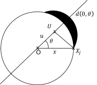
Figure 18: The tagged user at the origin, its serving base station $X_{j}$ at distance $x$ and a point $U$ at a distance $u$ on the line $d(0,\theta)$.

X-H Proof of Theorem 11

Proof.

Let $Z$ be a geometric random variable given by:

$$P(Z=l)=(1-\alpha)\alpha^{l}.$$ (57)

Then, the random variable $T$ representing the time taken to download the file is the geometric sum of independent random variables given by

$$T=\sum_{i=0}^{Z}(X_{i}+I^{(\gamma})+Y.$$ (58)

Thus, the Laplace transform of $T$ is

$$\begin{split}{\cal L}_{T}(s)&=\big{[}(1-\alpha)+(1-\alpha)\alpha{\cal L}_{X}(s){\cal L}_{I^{({\gamma})}}(s)+..\big{]}{\cal L}_{Y}(s)\\ \\ &=\frac{(1-\alpha){\cal L}_{Y}(s)}{1-\alpha{\cal L}_{X}(s){\cal L}_{I^{({\gamma})}}(s)}=\frac{(1-\alpha){\cal L}_{Y}(s)}{1-\alpha{\cal L}_{X}(s)\frac{2\lambda vr}{2\lambda vr+s}}.\end{split}$$ (59)

The last equality follows from the fact that the $I^{({\gamma})}$ is exponential with parameter $2\lambda vr$. ∎

Lemma 1.

For a $\mathbb{R^{+}}$ -valued random variable $U^{({\gamma})}$ defined by  (36) and service time distribution by  (5). We have the following limit:

$$\lim_{r_{\gamma}\to\infty}2\lambda r_{\gamma}v\mathbb{E}[U^{({\gamma})}]=1.$$

From Equations (7) and (36):

$$P[U^{({\gamma})}>u]=\frac{e^{-\rho^{({\gamma})}}}{\nu^{({\gamma})}}(e^{\rho^{({\gamma})}P[\hat{W}^{({\gamma})}>u]}-1),u\geq 0,$$ (60)

and

$$\begin{split}\mathbb{E}[U^{({\gamma})}]&=\int_{0}^{2r_{\gamma}/v}P[U^{({\gamma})}>u]du\\ \\ &=\frac{e^{-\rho^{({\gamma})}}}{\nu^{({\gamma})}}\int_{0}^{2r_{\gamma}/v}(e^{\rho^{({\gamma})}P[\hat{W}^{({\gamma})}>u]}-1)du.\end{split}$$ (61)

Thus,

$$\mathbb{E}[U^{({\gamma})}]=\frac{e^{-\rho^{({\gamma})}}}{\nu^{({\gamma})}}\bigg{(}\int_{0}^{2r/v}e^{\rho^{({\gamma})}P[\hat{W}^{({\gamma})}>u]}du-\frac{2r_{\gamma}}{v}\bigg{)}.$$ (62)

Since $\hat{W}^{({\gamma})}$ is the forward recurrence time associated with the service time $W^{({\gamma})}$ defined in  (6),

$$\mathbb{P}(\hat{W}^{({\gamma})}>u)=\frac{1}{\mathbb{E}[W^{({\gamma})}]}\int_{u}^{\infty}\mathbb{P}(W^{({\gamma})}>t)dt,$$

where, $\mathbb{E}[W^{({\gamma})}]=\frac{\rho^{({\gamma})}}{2r_{\gamma}v\lambda}$ from  (7) and $\mathbb{P}(W^{({\gamma})}>t)=1/2r_{\gamma}\sqrt{4r_{\gamma}^{2}-v^{2}t^{2}}$ from  (5).

Thus,

$$\begin{split}&\mathbb{E}[U^{({\gamma})}]=\frac{e^{-\rho^{({\gamma})}}}{\nu^{({\gamma})}}\bigg{(}\int_{0}^{\frac{2r_{\gamma}}{v}}e^{\lambda v\int_{u}^{\frac{2r_{\gamma}}{v}}\sqrt{4r_{\gamma}^{2}-v^{2}t^{2}}dt}du-\frac{2r_{\gamma}}{v}\bigg{)}\\ \\ &=\frac{e^{-\rho^{({\gamma})}}}{\nu^{({\gamma})}}\bigg{(}\int_{0}^{\frac{2r_{\gamma}}{v}}e^{\lambda\int_{u}^{2r_{\gamma}}\sqrt{4r_{\gamma}^{2}-x^{2}}dx}du-\frac{2r_{\gamma}}{v}\bigg{)}\\ \\ &=\frac{1}{\nu^{({\gamma})}}\bigg{(}\int_{0}^{\frac{2r_{\gamma}}{v}}e^{-\lambda(\frac{1}{2}u\sqrt{4r_{\gamma}^{2}-v^{2}u^{2}}+2r_{\gamma}^{2}{\arctan}(\frac{uv}{\sqrt{4r_{\gamma}^{2}-v^{2}u^{2}}})}du\\ \\ &~{}~{}~{}~{}-e^{-\lambda\pi r_{\gamma}^{2}}\frac{2r_{\gamma}}{v}\bigg{)}\\ \\ &=\frac{1}{1-e^{-\lambda\pi r_{\gamma}^{2}}}\bigg{(}\frac{r_{\gamma}}{v}\int_{0}^{2}e^{-\lambda r_{\gamma}^{2}q(z)}dz-\frac{2e^{-\lambda\pi r_{\gamma}^{2}}r_{\gamma}}{v}\bigg{)}.\end{split}$$ (63)

The second equality is by the change of variables $vt=x$ and the last equality is by the change of variables $z=uv/r_{\gamma}$ and $q(z)=\frac{1}{2}z\sqrt{4-z^{2}}+2{\arctan}(\frac{z}{\sqrt{4-z^{2}}})$.

Now, from Equation (63) we have,

$$\lim_{r_{\gamma}\to\infty}\mathbb{E}[U^{({\gamma})}]\sim\frac{r_{\gamma}}{v}\int_{0}^{2}e^{-\lambda r_{\gamma}^{2}q(z)}dz.$$

Now, the integral $\frac{r_{\gamma}}{v}\int_{0}^{2}e^{-\lambda r_{\gamma}^{2}q(z)}$ and $\frac{r_{\gamma}}{v}\int_{0}^{2}e^{-\lambda r_{\gamma}^{2}2z}dz$ are asymptotically equal as $r_{\gamma}$ goes to $\infty$.

The asymptotic equality of the two functions as $r_{\gamma}$ goes to $\infty$ means, that the relative error of the approximate equality goes to 0 as $r_{\gamma}$ goes to $\infty$ i.e.,

$$\lim_{r_{\gamma}\to\infty}\frac{\int_{0}^{2}e^{-\lambda r_{\gamma}^{2}q(z)}-e^{-\lambda r_{\gamma}^{2}2z}dz}{\int_{0}^{2}e^{-\lambda r_{\gamma}^{2}2z}}=0.$$

With the help of the Taylor series expansion, we get that

$$\lim_{r_{\gamma}\to\infty}\frac{\int_{0}^{C/r_{\gamma}^{2}}e^{-\lambda r_{\gamma}^{2}q(z)}-e^{-\lambda r_{\gamma}^{2}2z}dz}{\int_{0}^{2}e^{-\lambda r_{\gamma}^{2}2z}}=0,$$

for some constant $C$.

Thus, we need to prove that

$$\lim_{r_{\gamma}\to\infty}\frac{\int_{C/r_{\gamma}^{2}}^{2}e^{-\lambda r_{\gamma}^{2}q(z)}-e^{-\lambda r_{\gamma}^{2}2z}dz}{\int_{0}^{2}e^{-\lambda r_{\gamma}^{2}2z}}=0.$$

Now let us observe the function $h(z)=e^{-\lambda r_{\gamma}^{2}q(z)}-e^{-\lambda r_{\gamma}^{2}2z}$. The derivative of the function $h(z)$ is

$$\begin{split}h^{\prime}(z)&=\big{(}-\sqrt{4-z^{2}}e^{-\lambda r_{\gamma}^{2}q(z)}+2e^{-\lambda r_{\gamma}^{2}2z}\big{)}r_{\gamma}^{2}\\ \\ &=e^{-\lambda r_{\gamma}^{2}2z}r_{\gamma}^{2}\bigg{[}2-\sqrt{4-z^{2}}e^{-\lambda r^{2}[q(z)-2z]}\bigg{]}.\end{split}$$ (64)

Thus by substituting $z=C/r_{\gamma}^{2}$ and using the Taylor series expansion of $[q(z)-2z]$ and $\sqrt{4-z^{2}}$ , we get

$$\lim_{r_{\gamma}\to\infty}h^{\prime}(C/r_{\gamma}^{2})=e^{-2C\lambda z}[o(r_{\gamma})]=0.$$

The derivative of function $h(z)$ is 0 for $z=C/r_{\gamma}^{2}$ as $r_{\gamma}$ goes to $\infty$ i.e., the function $h(z)$ has a local maximum at $C/r_{\gamma}^{2}$ for some constant $C$ and it can be observed that it is decreasing for $C=3$.

Therefore, the function $h(z)$ is a decreasing function from $3/r_{\gamma}^{2}$ to 2 and the area under its curve has an upper bound that goes to 0.

Thus, the two integrals are asymptotically equal as $r_{\gamma}$ goes to $\infty$, which implies that $\mathbb{E}[U^{({\gamma})}]\sim\frac{1}{2vr_{\gamma}\lambda}$ as $r_{\gamma}$ goes to $\infty$.

References

- [1] Wandera, “Enterprise Mobile Data Report - q3,” Oct 2013. [Online]. Available: http://viroam.iroam.com/sites/all/themes/elegantica/documents/Enterprise%20Mobile%20Data%20Report%20-%20Q3.pdf
- [2] F. Baccelli and B. Blaszczyszyn, Spatial Modeling of Wireless Communications – A Stochastic Geometry Approach. NOW Publishers, 2009.
- [3] T. Karagiannis, J.-Y. Le Boudec, and M. Vojnović, “Power law and exponential decay of intercontact times between mobile devices,” Mobile Computing, IEEE Transactions on, 2010.
- [4] V. Conan, J. Leguay, and T. Friedman, “Characterizing pairwise inter-contact patterns in delay tolerant networks,” in Proceedings of the 1st international conference on Autonomic computing and communication systems. ICST, 2007.
- [5] H. Cai and D. Y. Eun, “Toward stochastic anatomy of inter-meeting time distribution under general mobility models,” in Proceedings of the 9th ACM international symposium on Mobile ad hoc networking and computing. ACM, 2008.
- [6] C.-H. Lee, J. Kwak et al., “Characterizing link connectivity for opportunistic mobile networking: Does mobility suffice?” in Proc. IEEE INFOCOM, 2013.
- [7] S. Mitra, S. Ranu, V. Kolar, A. Telang, A. Bhattacharya, R. Kokku, and S. Raghavan, “Trajectory aware macro-cell planning for mobile users,” arXiv preprint arXiv:1501.02918, 2015.
- [8] H. Deng and I.-H. Hou, “Online scheduling for delayed mobile offloading,” in Proc. IEEE INFOCOM, 2015.
- [9] Z. Lu and G. de Veciana, “Optimizing stored video delivery for mobile networks: The value of knowing the future,” in Proc. IEEE INFOCOM, 2013.
- [10] J. Keilson, Markov chain model-rarity and exponentiality. Springer Science & Business Media, 2012, vol. 28.
- [11] D. Aldous”, ”Probability Approximations via the Poisson Clumping Heuristic”. Springer-Verlag, 1989.
- [12] A. M. Makowski, “On a random sum formula for the busy period of the M/G/Infinity queue with applications,” DTIC Document, Tech. Rep., 2001. [Online]. Available: http://www.researchgate.net/publication/235086381_On_a_Random_Sum_Formula_for_the_Busy_Period_of_the_MGInfinity_Queue_With_Applications
- [13] S. N. Chiu, D. Stoyan, W. S. Kendall, and J. Mecke, Stochastic geometry and its applications. John Wiley & Sons, 2013.
- [14] A. Okabe, B. Boots, K. Sugihara, and S. N. Chiu, Spatial tessellations: concepts and applications of Voronoi diagrams. John Wiley & Sons, 2009.
- [15] J. Møller, “Random johnson-mehl tessellations,” Advances in applied probability, 1992.
- [16] E. W. Weisstein, “Kolmogorov-Smirnov test,” MathWorld–A Wolfram Web Resource. [Online]. Available: http://mathworld.wolfram.com/Kolmogorov-SmirnovTest.html
- [17] F. Baccelli and P. Brémaud, Palm probabilities and Stationary Queues. Springer Verlag, March 1987.
- [18] V. Gupta and P. G. Harrison, “Fluid level in a reservoir with an on-off source,” ACM SIGMETRICS Performance Evaluation Review, 2008.
- [19] J. F. C. Kingman, Poisson processes. Wiley Online Library, 1993.
- [20] F. Morlot, “A population model based on a poisson line tessellation,” in WiOpt’12: Modeling and Optimization in Mobile, Ad Hoc, and Wireless Networks. IEEE, 2012.
- [21] F. Baccelli, M. Klein, M. Lebourges, and S. Zuyev, “Stochastic geometry and architecture of communication networks,” Telecommunication Systems, 1997.