Formulation of the twisted-light–matter interaction at the phase singularity:
beams with strong magnetic fields

Abstract

The formulation of the interaction of matter with singular light fields needs special care. In a recent article [Phys. Rev. A 91, 033808 (2015)] we have shown that the Hamiltonian describing the interaction of a twisted light beam having parallel orbital and spin angular momenta with a small object located close to the phase singularity can be expressed only in terms of the electric field of the beam. Here, we complement our studies by providing an interaction Hamiltonian for beams having antiparallel orbital and spin angular momenta. Such beams may exhibit unusually strong magnetic effects. We further extend our formulation to radially and azimuthally polarized beams. The advantages of our formulation are that for all beams the Hamiltonian is written solely in terms of the electric and magnetic fields of the beam and as such it is manifestly gauge-invariant. Furthermore it is intuitive by resembling the well-known expressions in the dipole-electric and dipole-magnetic moment approximations.

I Introduction

Typically, when studying the interaction of light with nanometer-sized structures the characteristic length scale of the light field is much larger than the size of the structure. In this case it is usually sufficient to consider plane wave-like or spatially homogeneous beams. This does not hold anymore if the structure is placed at or close to a singular point of a light beam.

A prominent example for such a singular light beam is twisted light (TL), also called optical vortex light or light carrying orbital angular momentum, which has a phase singularity at the beam axis. A variety of new effects have been predicted and observed in the study of TL beams, spanning pure optics Andrews (2008); Ballantine et al. (2016); Yamane et al. (2012) and the interaction with atoms Köksal and Berakdar (2012); Surzhykov et al. (2015), molecules Wätzel et al. (2016), ions Schmiegelow and Schmidt-Kaler (2012); Peshkov et al. (2015), Bose-Einstein condensation Bhowmik et al. (2016), and solid-state systems Quinteiro and Tamborenea (2009a); Shigematsu et al. (2013); Clayburn et al. (2013); Noyan and Kikkawa (2015); Shintani et al. (2016); Koç and Köksal (2015). All these effects promise interesting new applications to material processing Omatsu et al. (2010), communications Spinello et al. (2016), lasers Zhang et al. (2016); Abulikemu et al. (2016); Miao et al. (2016), spintronics Quinteiro and Kuhn (2014) and particle manipulation Woerdemann et al. (2013).

Another class of spatially strongly inhomogeneous light beams are radially and azimuthally polarized beams, which can be realized as linear combinations of TL beams with opposite angular momentum and circular polarization. These beams have received much attention for their high potential in applications. Thanks to their strong longitudinal-field component with high intensity and degree of focusing, they prove useful in fields like micro-Raman spectroscopy Saito et al. (2008), material processing Wang et al. (2008); Meier et al. (2007), and as optical tweezers for metallic particles Zhan (2004). It was also suggested that a strong longitudinal component can help to excite intersubband transitions in quantum wells Sbierski et al. (2013) and light-hole states in quantum dots Quinteiro and Kuhn (2014). These states are technologically challenging to address, since conventional fields can only excite them if the beam propagates perpendicular to the growth direction of the sample, which typically requires cleaving the structure. From a theoretical perspective it has been also demonstrated that these fields can be classically entangled in a way similar to what we find in quantum mechanical systems Gabriel et al. (2011).

It is becoming increasingly clear that the interaction of highly inhomogeneous light fields, and in particular of singular fields like TL Dennis et al. (2009), with atoms or solids is non-trivial and needs special care in the theoretical description. Here, the widely used dipole-moment approximation cannot be applied anymore. Of course, one can always work with the minimal coupling Hamiltonian; however, its use entails some disadvantages, for example it lacks direct connection to the electro-magnetic fields, the real quantities accessible in experiments. In Ref. Quinteiro et al. (2015), we have shown recently that the formulation of the light-matter interaction had to be revisited and demonstrated that previous formulations meant for smooth fields are not the most suitable ones to treat TL, especially when the interaction with small structures close to the phase singularity is considered. Using elementary gauge transformations, we further developed a new gauge –the TL gauge– which allowed us to cast the Hamiltonian in a form containing the electric field only.

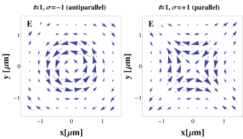
Figure 1: Electric field profile in the $xy$-plane for parallel and antiparallel TL propagating along the $z$-direction. We chose the topological charge to $\ell=1$ and the handedness of polarisation to $\sigma=1$ (left) and $\sigma=-1$ (right).

Though having an appealing form, the TL gauge developed in Ref. Quinteiro et al. (2015) is only applicable to a certain subclass of TL beams, which can be explained as follows: TL beams can be discriminated into two topologically different classes depending on the combination of circular polarization (or spin angular momentum) and topological charge (or orbital angular momentum). If circular polarization and topological charge have the same sign, we call this the parallel class, while for opposite sign the beams are called antiparallel. One example of the electric field profile for the two classes is shown in Fig. 1. One can immediately see the difference in the spatial profiles of the beams, which even by evolving in time will not transform into each other. Coming back to the TL-matter interaction, we have shown that the TL gauge can only be applied to the parallel class Quinteiro et al. (2015) since it does not account for a magnetic coupling, which turns out to be crucial in the antiparallel class.

In this paper we extend the description of the TL-matter interaction to the family of antiparallel TL beams by including both electric and magnetic interaction terms. We will show that for antiparallel beams with orbital angular momentum larger than one the magnetic interaction becomes unusually strong. The formulation can also be directly applied to the interaction of radially or azimuthally polarized beams with small structures close to the beam center. The light-matter Hamiltonian derived here shares the benefits of our previous TL gauge, namely, it is intuitive and easy to use. Thereby, this article completes the gauge invariance formulation of the TL-matter interaction close to the phase singularity.

We organize the article as follows. Section II describes the modes of twisted light, providing the expressions for electric and magnetic fields close to the phase singularity. Like in our previous paper we will restrict the explicit formulas to Bessel modes. Since the derivation only relies on the behavior close to the phase singularity, however, the general features are also valid for other types of beams like, e.g., Laguerre-Gauss (LG) beams. The derivation and formulation of the TL–matter Hamiltonian in terms of electric and magnetic fields is given in Sect. III followed by a discussion of the resulting Hamiltonain in Sect. IV. Section V treats the case of radially and azimuthally polarized fields. The conclusions are presented in Sect. VI.

II Bessel singular fields

The most significant feature of TL is its topological charge $\ell$ that adds orbital angular momentum via the phase $\exp(i\ell\varphi)$, where $\varphi$ is the angle in the cylindrical coordinates $\{r,\varphi,z\}$ for a beam centered around $r=0$ and propagating in the $z$-direction. This implies a phase singularity at $r=0$ whenever $\ell\neq 0$. Another important parameter is the handedness of the circular polarization denoted by $\sigma=\pm 1$. The combination of the signs of $\ell$ and $\sigma$ leads to the distinction into the parallel [sign($\sigma$)=sign($\ell$)] and the antiparallel [sign($\sigma$) $\neq$ sign($\ell$)] classes. In the radial modes one distinguishes between LG and Bessel modes. The main difference between these types is their radial localization, i.e., their behavior for large values of $r$. Close to the beam axis they behave similarly. In this paper we will restrict ourselves to the case of Bessel beams because they are exact solutions of the full Helmholtz equation Volke-Sepulveda et al. (2002) and therefore can be applied also beyond the limits of the paraxial approximation. Furthermore they are non-diffracting beams, such that the radial profiles are independent of the propagation coordinate $z$.

Bessel beams can be derived from the vector potential in the Coulomb gauge, as explained in App. A. We are interested in the description of the light-matter interaction close to the phase singularity. Thus, we approximate the full fields given in App. A in the region $q_{r}r\ll 1$, where $1/q_{r}$ is a measure of the beam radius. This is basically done by expanding the Bessel functions $J_{\ell}(q_{r}r)\propto(q_{r}r)^{|\ell|}$ Quinteiro et al. (2015). To simplify the notation here we will assume $\ell>0$. The extension to negative values is straightforward. Note that the formulas for the full fields given in App. A hold for arbitrary values of $\ell$.

Separating the propagating phase from the mode functions according to $\textbf{E}(\textbf{r},t)=\frac{1}{2}\tilde{\textbf{E}}(\textbf{r})e^{i(q_{z}z-\omega t)}+\textrm{c.c.}$ and $\textbf{B}(\textbf{r},t)=\frac{1}{2}\tilde{\textbf{B}}(\textbf{r})e^{i(q_{z}z-\omega t)}+\textrm{c.c.}$, where c.c. denotes the complex conjugate, the electric field for circular polarization $\sigma=\pm 1$ reads

$$\tilde{E}_{x}(\mathbf{r}) = i\frac{E_{0}}{2^{\ell}\ell!}(q_{r}r)^{\ell}e^{i\ell\varphi}$$ (1a)

$$\tilde{E}_{y}(\mathbf{r}) = -\sigma\frac{E_{0}}{2^{\ell}\ell!}(q_{r}r)^{\ell}e^{i\ell\varphi}$$ (1b)

$$\tilde{E}_{z}(\mathbf{r}) = \sigma\frac{E_{0}}{2^{\ell+\sigma}(\ell+\sigma)!}\frac{q_{r}}{q_{z}}(q_{r}r)^{\ell+\sigma}e^{i(\ell+\sigma)\varphi}\hskip 19.91692pt$$ (1c)

with the electric field amplitude $E_{0}$, the frequency $\omega$, and the wave vector components $q_{z}$ and $q_{r}$. The latter quantities are related by $q_{z}^{2}+q_{r}^{2}=(n\omega/c)^{2}$, $n$ being the index of refraction of the medium.

From Eqs. (1) we already notice a qualitative difference between the parallel and the antiparallel class: While in the parallel class the electric field close to the origin is dominantly in-plane, in the antiparallel class the $z$-component becomes dominant. The differences are even more pronounced in the case of the magnetic field which for $\sigma=+1$ (parallel class) is given by

$$\tilde{B}_{x}(\mathbf{r}) = \frac{B_{0}}{2^{\ell}\ell!}\left[1+\frac{1}{2}\left(\frac{q_{r}}{q_{z}}\right)^{2}\right]\left(q_{r}r\right)^{\ell}e^{i\ell\varphi}\hskip 19.91692pt$$ (2a)

$$\tilde{B}_{y}(\mathbf{r}) = i\frac{B_{0}}{2^{\ell}\ell!}\left[1+\frac{1}{2}\left(\frac{q_{r}}{q_{z}}\right)^{2}\right]\left(q_{r}r\right)^{\ell}e^{i\ell\varphi}$$ (2b)

$$\tilde{B}_{z}(\mathbf{r}) = -i\frac{B_{0}}{2^{\ell+1}(\ell+1)!}\frac{q_{r}}{q_{z}}\left(q_{r}r\right)^{\ell+1}e^{i(\ell+1)\varphi}\,,$$ (2c)

with $B_{0}=(q_{z}/\omega)E_{0}$, while for $\sigma=-1$ (antiparallel class) it reads

$$\tilde{B}_{x}(\mathbf{r}) = -\frac{B_{0}}{2^{\ell}\ell!}\left\{\left[1+\frac{1}{2}\left(\frac{q_{r}}{q_{z}}\right)^{2}\right]-\frac{\ell}{2}\left(\frac{q_{r}}{q_{z}}\right)^{2}e^{-i2\varphi}\right.$$ (3a)

$$\left.+\frac{1}{2}\left(\frac{q_{r}}{q_{z}}\right)^{2}\frac{4\ell(\ell-1)}{(q_{r}r)^{2}}e^{-i2\varphi}\right\}(q_{r}r)^{\ell}e^{i\ell\varphi}$$

$$\tilde{B}_{y}(\mathbf{r}) = i\frac{B_{0}}{2^{\ell}\ell!}\left\{\left[1+\frac{1}{2}\left(\frac{q_{r}}{q_{z}}\right)^{2}\right]+\frac{\ell}{2}\left(\frac{q_{r}}{q_{z}}\right)^{2}e^{-i2\varphi}\right.$$ (3b)

$$\left.-\frac{1}{2}\left(\frac{q_{r}}{q_{z}}\right)^{2}\frac{4\ell(\ell-1)}{(q_{r}r)^{2}}e^{-i2\varphi}\right\}(q_{r}r)^{\ell}e^{i\ell\varphi}$$

$$\tilde{B}_{z}(\mathbf{r}) = -i\frac{B_{0}}{2^{\ell-1}(\ell-1)!}\frac{q_{r}}{q_{z}}(q_{r}r)^{\ell-1}e^{i(\ell-1)\varphi}\,.$$ (3c)

For the magnetic field, the dependence on $r$ is strongly modified by the combination of polarization and topological charge. In the parallel class it behaves similar to the electric field; in particular the in-plane components dominate and vary as $(q_{r}r)^{\ell}$. In the antiparallel class for $\ell=1$, like in the case of the electric field, the $z$-component becomes dominant behaving as $(q_{r}r)^{(\ell-1)}$. Even more interesting, for antiparallel beams with $\ell\geq 2$ there are second-order terms in the ratio $(q_{r}/q_{z})$ proportional to $(q_{r}r)^{\ell-2}$ in the in-plane components. Being solutions of the full wave equation, for Bessel beams $(q_{r}/q_{z})$ may take any value, and such terms may become important under strong focussing. This is the reason why one cannot write the interaction Hamiltonian only in terms of electric fields, as can be done in the TL gauge for beams in the parallel class Quinteiro et al. (2015).

III Formulating the interaction in terms of electric and magnetic fields

We derive the TL-matter Hamiltonian in the Poincaré gauge. The starting point are the general formulas Cohen-Tannoudji et al. (1989)

$$\mathbf{A}(\mathbf{r},t) = -\int_{0}^{1}\,du\,u\,\mathbf{r}\times\mathbf{B}(u\mathbf{r},t)$$ (4a)

$$U(\mathbf{r},t) = -\int_{0}^{1}\,du\,\mathbf{r}\cdot\mathbf{E}(u\mathbf{r},t)\,.$$ (4b)

These potentials are inserted in the standard minimal coupling Hamiltonian

$$H=\frac{1}{2m}[\mathbf{p}-q\mathbf{A}(\mathbf{r},t)]^{2}+V(\mathbf{r})+qU(\mathbf{r},t),$$ (5)

where $V(\mathbf{r})$ denotes a static potential for the particles with charge $q$ and mass $m$. Assuming that the term proportional to $\mathbf{A}^{2}$ is negligible, which is well justified for typical magnetic field strengths in a light beam, the coupling to the electric field is then described by the Hamiltonian

$$H_{e}=qU(\mathbf{r},t)$$ (6)

while for the coupling to the magnetic field we obtain

$$H_{m} = -\frac{q}{2m}\left[\mathbf{p}\cdot\mathbf{A}(\mathbf{r},t)+\mathbf{A}(\mathbf{r},t)\cdot\mathbf{p}\right]\,.$$ (7)

We are interested in the interaction of the beam with flat, nano-sized structures with radial extensions much smaller than the beam waist located around $z=0$ and $r=0$. Therefore, we can use the approximate field profiles of Eqs. (1)-(3) and take the propagating phase factor at $z=0$. We adopt the convention $\mathbf{r}_{\perp}=r\hat{\mathbf{r}}$.

III.1 Electric interaction

We first consider the interaction with the electric field, for which we already derived the TL gauge for the parallel class. Using the electric field from Sec. II we can easily evaluate the integral in Eq. (4b). Note, that the transverse components of the parallel and antiparallel beams have the same $r$-dependence $(q_{r}r)^{|\ell|}$, while for the $z$ component $(q_{r}r)^{|\ell+\sigma|}$. In total, according to Eq. (6) the electric Hamiltonian for the interaction with a particle with charge $q$ is

$$H_{e} = -\frac{1}{|\ell|+1}\,q\mathbf{r}_{\perp}\cdot\mathbf{E}_{\perp}(\mathbf{r}_{\perp},t)$$ (8)

$$-\frac{1}{|\ell+\sigma|+1}\,qz\,E_{z}(\mathbf{r}_{\perp},t)\,,$$

where $\mathbf{E}_{\perp}=(E_{x},E_{y})$, and we call $q\mathbf{r}_{\perp}$ the in-plane dipole moment $\mathbf{d}$, although the interaction is actually multipolar. We also want to stress the appearance of the prefactors due to the vortex structure of the field. Equation (8) is in agreement with our previous results Quinteiro et al. (2015), but is valid for the parallel and antiparallel classes.

Next, we want to check, whether the approximation $z=0$ assuming a flat structure holds. For this, we include the next order of the Taylor expansion in $z$ of the field, $\textbf{E}(\textbf{r},t)\approx\frac{1}{2}\tilde{\textbf{E}}(\mathbf{r}_{\perp})[1+iq_{z}z]e^{-i\omega t}+\textrm{c.c.}$. Also for this field Eq. (4b) can be readily evaluated giving rise to a second order contribution to the interaction Hamiltonian according to

$$H_{e}^{(2)} \sim -q_{z}\frac{1}{|\ell|+1}\,qz\mathbf{r}_{\perp}\cdot\mathbf{E}_{\perp}(\mathbf{r}_{\perp},t)$$ (9)

$$-q_{z}\frac{q}{|\ell+\sigma|+2}\,qz^{2}\,E_{z}(\mathbf{r}_{\perp},t)\,,$$

As example we could think of a planar nanostructure excited by optical fields. For instance a disk-shaped QD Quinteiro and Tamborenea (2009b) with $2-5$ nm height impinged at normal incidence by a light pulse of $q_{z}=2\pi/\lambda=0.01$nm^-1 yields $q_{z}|z|<0.05$. Indeed, we see that the first term dominates, which is ensured by the condition $q_{z}|z|\ll 1$. It is worth mentioning that there are situations in which higher orders are required; for instance, due to the parity of the initial $\Psi_{i}$ and final $\Psi_{f}$ states involved in the optical transition, the term $\langle{\Psi_{f}}|\,\{-[1/(|\ell|+1)]\,\mathbf{r}_{\perp}\cdot\mathbf{E}_{\perp}(\mathbf{r}_{\perp},t)\}\,|{\Psi_{i}}\rangle$ might be zero.

III.2 Magnetic (orbital) interaction

Now we turn to the interaction induced by the magnetic parts of the field.

Using Eqs. (4a) and (7) as well as the identities $\mathbf{p}\cdot(\mathbf{r}\times\mathbf{B})=(\mathbf{p}\times\mathbf{r})\cdot\mathbf{B})$ and $(\mathbf{r}\times\mathbf{B})\cdot\mathbf{p}=\mathbf{B}\cdot(\mathbf{p}\times\mathbf{r})$, we obtain

$$H_{m} = \frac{q}{2m}(\mathbf{p}\times\mathbf{r})\cdot\int_{0}^{1}\,du\,u\,\mathbf{B}(u\mathbf{r}_{\perp},t)$$ (10)

$$+\frac{q}{2m}\int_{0}^{1}\,du\,u\,\mathbf{B}(u\mathbf{r}_{\perp},t)\,\cdot\left(\mathbf{p}\times\mathbf{r}\right)\,.$$

Using that the commutator $[\mathbf{B}(\mathbf{r},t),(\mathbf{p}\times\mathbf{r})]$ is small (see Appendix B), we put together both terms in Eq. (10) simplifying our interaction to

$$H_{m} = \frac{q}{m}\left[\int_{0}^{1}\,du\,u\,\mathbf{B}(u\mathbf{r}_{\perp},t)\,\right]\cdot\left(\mathbf{p}\times\mathbf{r}\right)\,.$$ (11)

Inserting the magnetic fields from Sec. II, the evaluation of the integral is straightforward, resulting in

$$H_{m} = \frac{2}{|\ell|+2-j}\mathbf{B}_{\perp}(\mathbf{r}_{\perp},t)\cdot\left[\frac{q}{2m}(\mathbf{p}\times\mathbf{r})\right]$$ (12)

$$+\frac{2}{|\ell+\sigma|+2}B_{z}(\mathbf{r}_{\perp},t)\hat{\mathbf{z}}\cdot\left[\frac{q}{2m}(\mathbf{p}\times\mathbf{r})\right]\,,$$

with $j=2$ for antiparallel beams with $\ell\geq 2$ and $j=0$ otherwise.

We will call $[-(q/2m)(\mathbf{p}\times\mathbf{r})]$ the magnetic moment $\mathbf{m}_{B}$ keeping in mind that the interaction terms is a multipolar interaction. Of course, in the simplest case of homogeneous fields $\mathbf{B}(0,t)$ one recovers the well-known magnetic-dipole interaction $H_{m}=-\mathbf{m}_{B}\cdot\mathbf{B}(0,t)$.

IV Analyzing the Hamiltonian

For compactness and to reinforce the resemblance with well-known formulas used for smooth fields, we may define effective fields

$$\mathbf{E}^{\mathrm{eff}}(\mathbf{r}_{\perp},t) = \frac{1}{|\ell|+1}\,\mathbf{E}_{\perp}(\mathbf{r}_{\perp},t)$$

$$+\frac{1}{|\ell+\sigma|+1}\,E_{z}(\mathbf{r}_{\perp},t)\hat{\mathbf{z}}$$

$$\mathbf{B}^{\mathrm{eff}}(\mathbf{r}_{\perp},t) = \frac{2}{|\ell|+2-j}\mathbf{B}_{\perp}(\mathbf{r}_{\perp},t)$$

$$+\frac{2}{|\ell+\sigma|+2}B_{z}(\mathbf{r}_{\perp},t)\hat{\mathbf{z}}\,,$$

that allow us to write the complete Hamiltonian in an appealing form

$$H = \frac{\mathbf{p}^{2}}{2m}+V(\mathbf{r})-\mathbf{E}^{\mathrm{eff}}(\mathbf{r}_{\perp},t)\cdot\mathbf{d}$$ (13)

$$-\mathbf{B}^{\mathrm{eff}}(\mathbf{r}_{\perp},t)\cdot\mathbf{m}_{B}\,,$$

for it is local depending solely in the position vector $\mathbf{r}$ and is intuitive reminding the well-known dipole-moment interactions. We next discuss some features of our gauge as well some separate cases to illustrate the effects of TL-matter interaction.

IV.1 Comparison to the multipolar expansion:

Using simple arguments the Hamiltonian Eq. (13) can be compared to the multipolar expansion Cohen-Tannoudji et al. (1989). When expanding the electric field terms in Eq. (IV) we regain the lowest order multipolar terms. For example if $\ell=1$ the transverse electric field $E_{\perp}(\mathbf{r},t)\propto(q_{r}r)$ and the interaction $H_{e}=-\frac{1}{2}\mathbf{r}_{\perp}\cdot\mathbf{E}_{\perp}(\mathbf{r},t)\propto r^{2}$ is electric quadrupolar in $r$. If the OAM is increased to $\ell=2$, the interaction becomes $H_{e}\propto r^{3}$, an electric octupole. This is in agreement with our previous findings Quinteiro et al. (2015).

IV.2 Transverse ($xy$)-components:

In the paraxial approximation and also in most cases of interest, the transverse components of the fields play the major role. In this case, the Hamiltonian reduces to the simple form

$$H^{\perp}_{\textrm{int}} = -\frac{1}{|\ell|+1}\,\mathbf{E}_{\perp}(\mathbf{r}_{\perp},t)\cdot\mathbf{d}$$ (14)

$$-\frac{2}{|\ell|+2-j}\mathbf{B}_{\perp}(\mathbf{r}_{\perp},t)\cdot\mathbf{m}_{B}\,.$$

For the parallel class it can be shown that the electric component always dominates. For this, we remind the reader that the magnetic-$2^{n}$-pole interaction is weaker than the electric-$2^{n}$-pole interaction. This is clearly the case for homogeneous fields: with the use of $\langle\mathbf{p}\rangle=-i(m/\hbar)\langle[\mathbf{r},H_{0}]\rangle$ the magnetic-dipole interaction $-\mathbf{m}_{B}\cdot\mathbf{B}(0,t)\propto|({\mathbf{r}}\times{\mathbf{p}})|\propto\langle r\rangle^{2}$ while the electric-dipole interaction $-\mathbf{d}\cdot\mathbf{E}(0,t)\propto\langle r\rangle$. For parallel beams of TL, the $r$-dependence of magnetic and electric fields is the same $[(q_{r}r)^{\ell}]$, and the argument for homogeneous fields can be used to assert that the strongest interaction is the electric one.

For the antiparallel class, one has to be more careful and reconsider the fields given in Eqs. (1) and (3). For $\ell$=1 both fields are proportional to $r$ and for the same arguments as above, the electric field dominates. More interesting is the case $\ell=2$. On the one hand, the electric interaction is $\mathbf{d}\cdot\mathbf{E}(\mathbf{r},t)\propto r(q_{r}\,r)^{2}\propto r^{3}$, an electric octupole. On the other hand, the magnetic field is constant (no singularity), and its interaction is thus magnetic dipolar with $\mathbf{B}(\mathbf{r},t)\cdot(\mathbf{p}\times\mathbf{r})\propto\langle r\rangle^{2}$. This indicates that the magnetic interaction dominates close to $r=0$. Our conclusion is supported by Zurita’s et al. Zurita-Sánchez and Novotny (2002) study on the interaction of spherical QD with focused azimuthally polarized beam, where the transition rate is larger for the magnetic interaction. For the cases $\ell>2$, we also find that the magnetic field, which is proportional to $r^{\ell-2}$ overcomes the electric field, proportional to $r^{\ell}$.

In contrast to the TL gauge, the Hamiltonian in Eq. (14) accounts for both electric and magnetic field and is therefore able to capture all cases of handedness of polarization $\sigma$ and topological charge $\ell$.

IV.3 Longitudinal ($z$)-component:

The interaction Hamiltonian for the $z$-components of the field can be written as follows

$$H^{z}_{\mathrm{int}} = -\frac{1}{|\ell+\sigma|+1}\,E_{z}(\mathbf{r}_{\perp},t)d_{z}$$ (15)

$$-\frac{2}{|\ell+\sigma|+2}B_{z}(\mathbf{r}_{\perp},t)m_{B,z}\,.$$

For the $z$-components of the field, using the same arguments as above, the electric field dominates over the magnetic one in all cases.

V Extension to radially and azimuthally polarized fields

Radially and azimuthally polarized beams can be built as a superposition of two antiparallel twisted light beams having $\{\ell=1,\sigma=-1\}$ and $\{\ell=-1,\sigma=1\}$. Azimuthally polarized fields are given by the sum of these beams. In the approximation of small $r$ the fields read

$$E^{\mathrm{(az)}}_{\varphi} = E_{0}(q_{r}r)e^{i(q_{z}z-\omega t)}+\textrm{c.c.}$$

$$E^{\mathrm{(az)}}_{r} = E^{\mathrm{(az)}}_{z}=0\,,$$ (16)

and

$$B^{\mathrm{(az)}}_{r}(\textbf{r},t) = -B_{0}(q_{r}r)e^{i(q_{z}z-\omega t)}+\textrm{c.c.}$$

$$B^{\mathrm{(az)}}_{\varphi}(\textbf{r},t) = 0$$

$$B^{\mathrm{(az)}}_{z}(\textbf{r},t) = -2iB_{0}\frac{q_{r}}{q_{z}}e^{i(q_{z}z-\omega t)}+\textrm{c.c.}\,.$$ (17)

Likewise the radially polarized fields given by the difference of the two antiparallel beams are

$$E^{\mathrm{(rad)}}_{r}(\textbf{r},t) = iE_{0}(q_{r}r)e^{i(q_{z}z-\omega t)}+\textrm{c.c.}$$

$$E^{\mathrm{(rad)}}_{\varphi}(\textbf{r},t) = 0$$

$$E^{\mathrm{(rad)}}_{z}(\textbf{r},t) = -2\frac{q_{r}}{q_{z}}E_{0}e^{i(q_{z}z-\omega t)}+\textrm{c.c.}\,,$$ (18)

and

$$B^{\mathrm{(rad)}}_{\varphi}(\textbf{r},t) = iB_{0}\left[1+\left(\frac{q_{r}}{q_{z}}\right)^{2}\right](q_{r}r)e^{i(q_{z}z-\omega t)}+\textrm{c.c.}$$

$$B^{\mathrm{(rad)}}_{r}(\textbf{r},t) = B^{\mathrm{(rad)}}_{z}=0\,.$$ (19)

Evidently, for both types of fields all in-plane components, varying as $(q_{r}r)$, vanish at the origin. In contrast, at $r=0$ the azimuthally polarized beam is characterized by a non-vanishing $z$-component of the magnetic field while the radially polarized beam exhibits a non-vanishing $z$-component of the electric field. Thus, close to the beam center both fields are dominated by their longitudinal contributions.

Due to the particular mixture of polarization and topological charge the prefactors containing $|\ell+\sigma|$ and $|\ell|$ in Eqs. (8) and (12) are the same for each single $\{\ell,\sigma\}$ field. Thus, radially and azimuthally polarized beams can be directly used in the Hamiltonian expression Eq. (13). Working out the interaction terms for the $z$-components of the fields, we find for the radially polarized field

$$H_{e} = -E^{\mathrm{(rad)}}_{z}(\mathbf{r}_{\perp},t)\,d_{z}\,,$$ (20)

and for the azimuthally polarized field

$$H_{m} = -B^{\mathrm{(az)}}_{z}(\mathbf{r}_{\perp},t)\,m_{B,z}\,.$$ (21)

Note that there is no prefactor, since all $z$-components have no phase singularity.

VI Conclusions

We have revisited the mathematical formulation of the TL-matter interaction close to the phase singularity. In follow-up to the TL gauge Quinteiro et al. (2015), we have extended the gauge-invariant formulation by applying a transformation to the Poincaré gauge to both classes (parallel and antiparallel) of TL as well as to azimuthally and radially polarized beams. The Hamiltonian includes both electric and magnetic interaction, which is important, because for a particular combination of orbital and spin momenta the TL-matter interaction is dominated by the magnetic field, a very uncommon situation in optics. An important advantage of the Hamiltonian is that it is written solely in terms of fields, overcoming issues of gauge invariances. The expression is both local and intuitive, resembling well-known formulas used to study smooth light fields.

VII Acknowledgment

G. F. Quinteiro would like to thank the Argentine research agency Agencia Nacional de Promocion Cientifica y Tecnologica and the Institut für Festkörpertheorie of WWU Münster (Germany) for financial support.

Appendix A Potential and fields for Bessel beams

Using again the separation of the propagating phase from the mode function according to $\textbf{A}(\textbf{r},t)=\frac{1}{2}\tilde{\textbf{A}}(\textbf{r})e^{i(q_{z}z-\omega t)}+\textrm{c.c.}$, the vector potential of Bessel beams is Quinteiro et al. (2015)

$$\tilde{\textbf{A}}(\mathbf{r}) = A_{0}\,\left[\mathbf{e}_{\sigma}J_{\ell}(q_{r}r)e^{i\ell\varphi}\right.$$ (22)

$$\left.-i\,\sigma\mathbf{e}_{z}\frac{q_{r}}{q_{z}}J_{\ell+\sigma}(q_{r}r)e^{i(\ell+\sigma)\varphi}\right]\,,$$

with frequency $\omega$, wave vectors $q_{z}$ and $q_{r}$, related by $q_{z}^{2}+q_{r}^{2}=(n\omega/c)^{2}$, $A_{0}$ the amplitude and $n$ being the index of refraction of the medium. $J_{\ell}$ denotes the Bessel function and $\mathbf{e}_{\sigma}=(\mathbf{e}_{x}+i\sigma\mathbf{e}_{y})$ is the polarization with $\mathbf{e}_{x}$ ($\mathbf{e}_{y}$) is the unit vector in $x$ ($y$) direction. The scalar potential can be chosen to $\Phi(\textbf{r},t)=0$, such that the fields are calculated in the standard way via $\mathbf{E}=-\frac{\partial}{\partial t}\mathbf{A}$ and $\mathbf{B}=\nabla\times A$, which for the electric field yields

$$\tilde{E}_{x}(\mathbf{r}) = iE_{0}J_{\ell}(q_{r}r)e^{i\ell\varphi}\,,$$ (23a)

$$\tilde{E}_{y}(\mathbf{r}) = -\sigma E_{0}J_{\ell}(q_{r}r)e^{i\ell\varphi}\,,$$ (23b)

$$\tilde{E}_{z}(\mathbf{r}) = \sigma E_{0}\frac{q_{r}}{q_{z}}J_{\ell+\sigma}(q_{r}r)e^{i(\ell+\sigma)\varphi}\,,$$ (23c)

with $E_{0}=\omega A_{0}$. The magnetic field reads

$$\tilde{B}_{x}(\mathbf{r}) = \sigma B_{0}\biggl{[}\Bigl{(}1+\frac{q_{r}^{2}}{2q_{z}^{2}}-\frac{q_{r}^{2}}{2q_{z}^{2}}e^{i2\sigma\varphi}\Bigr{)}J_{\ell}(q_{r}r)e^{i\ell\varphi}$$ (24a)

$$+\frac{q_{r}^{2}}{2q_{z}^{2}}(\ell+\sigma)\frac{2}{q_{r}r}J_{\ell+\sigma}(q_{r}r)e^{i(\ell+2\sigma)\varphi}\biggr{]}\,,$$

$$\tilde{B}_{y}(\mathbf{r}) = iB_{0}\biggl{[}\Bigl{(}1+\frac{q_{r}^{2}}{2q_{z}^{2}}+\frac{q_{r}^{2}}{2q_{z}^{2}}e^{i2\sigma\varphi}\Bigr{)}J_{\ell}(q_{r}r)e^{i\ell\varphi}$$ (24b)

$$-\frac{q_{r}^{2}}{2q_{z}^{2}}(\ell+\sigma)\frac{2}{q_{r}r}J_{\ell+\sigma}(q_{r}r)e^{i(\ell+2\sigma)\varphi}\biggr{]}\,,$$

$$\tilde{B}_{z}(\mathbf{r}) = -iB_{0}\frac{q_{r}}{q_{z}}J_{\ell+\sigma}(q_{r}r)e^{i(\ell+\sigma)\varphi}\,,$$ (24c)

with $B_{0}=q_{z}A_{0}=(q_{z}/\omega)E_{0}$. The behavior close to the beam center given in Sec. II is obtained from the expansion

$$J_{\nu}(z)=\frac{z^{\nu}}{2^{\nu}\nu!}\left[1-\frac{z^{2}}{4(\nu+1)}+\dots\right]$$ (25)

valid for $\nu\geq 0$ and the relation $J_{-\nu}(z)=(-1)^{\nu}J_{\nu}(x)$.

Appendix B Commutator $[\mathbf{B}(\mathbf{r},t),(\mathbf{p}\times\mathbf{r})]$

Considering linear materials and that $\mathbf{p}\times\mathbf{r}=-\mathbf{r}\times\mathbf{p}$

$$[\mathbf{B}(\mathbf{r},t),(\mathbf{p}\times\mathbf{r})] = \mathbf{r}\cdot[\mathbf{p}\times\mathbf{B}(\mathbf{r},t)]$$ (26)

$$= -i\hbar\mathbf{r}\cdot[\nabla\times\mathbf{B}(\mathbf{r},t)]$$

$$= -i\hbar\mu\epsilon\mathbf{r}\cdot\frac{\partial\mathbf{E}(\mathbf{r},t)}{\partial t}\,,$$

where in the last line we used Ampere-Maxwell’s equation and the fact that the current $\mathbf{j}(\mathbf{r},t)$ –source of $E$ and $B$– is far away and can be disregarded. For a monochromatic field $\partial_{t}\mathbf{E}(\mathbf{r},t)=-i\omega\mathbf{E}(\mathbf{r},t)$ and $\mu\epsilon=1/c^{2}$, then the correction to the magnetic Hamiltonian $H_{m}$ is

$$\Delta H_{m} = \int_{0}^{1}du\,u\,\frac{q}{2m}[\mathbf{B}(u\mathbf{r},t),(\mathbf{p}\times\mathbf{r})]$$ (27)

$$= -\frac{q}{2}\frac{\hbar\omega}{mc^{2}}\int_{0}^{1}du\,u^{2}\mathbf{r}\cdot\mathbf{E}(u\mathbf{r},t)\,.$$

Thus, the correction has a structure similar to the electric Hamiltonion, however with a prefactor $\hbar\omega/(mc^{2})\simeq 10^{-5}$. It can therefore be safely disregarded.

References

- Andrews (2008) D. L. Andrews, Structured light and its applications: An introduction to phase-structured beams and nanoscale optical forces (Academic Press, 2008).
- Ballantine et al. (2016) K. E. Ballantine, J. F. Donegan, and P. R. Eastham, Science Advances 2, e1501748 (2016).
- Yamane et al. (2012) K. Yamane, Y. Toda, and R. Morita, Optics express 20, 18986 (2012).
- Köksal and Berakdar (2012) K. Köksal and J. Berakdar, Phys. Rev. A 86, 063812 (2012).
- Surzhykov et al. (2015) A. Surzhykov, D. Seipt, V. Serbo, and S. Fritzsche, Phys. Rev. A 91, 013403 (2015).
- Wätzel et al. (2016) J. Wätzel, Y. Pavlyukh, A. Schäffer, and J. Berakdar, Carbon 99, 439 (2016).
- Schmiegelow and Schmidt-Kaler (2012) C. T. Schmiegelow and F. Schmidt-Kaler, The European Physical Journal D 66, 1 (2012).
- Peshkov et al. (2015) A. Peshkov, S. Fritzsche, and A. Surzhykov, Physical Review A 92, 043415 (2015).
- Bhowmik et al. (2016) A. Bhowmik, P. K. Mondal, S. Majumder, and B. Deb, Physical Review A 93, 063852 (2016).
- Quinteiro and Tamborenea (2009a) G. F. Quinteiro and P. I. Tamborenea, Europhys. Lett. 85, 47001 (2009a).
- Shigematsu et al. (2013) K. Shigematsu, Y. Toda, K. Yamane, and R. Morita, Jpn. J. Appl. Phys. 52, 08JL08 (2013).
- Clayburn et al. (2013) N. B. Clayburn, J. L. McCarter, J. M. Dreiling, M. Poelker, D. M. Ryan, and T. J. Gay, Phys. Rev. B 87, 035204 (2013).
- Noyan and Kikkawa (2015) M. A. Noyan and J. M. Kikkawa, Appl. Phys. Lett. 107, 032406 (2015).
- Shintani et al. (2016) K. Shintani, K. Taguchi, Y. Tanaka, and Y. Kawaguchi, Phys. Rev. B 93, 195415 (2016).
- Koç and Köksal (2015) F. Koç and K. Köksal, Superlattices and Microstructures 85, 599 (2015).
- Omatsu et al. (2010) T. Omatsu, K. Chujo, K. Miyamoto, M. Okida, K. Nakamura, N. Aoki, and R. Morita, Optics express 18, 17967 (2010).
- Spinello et al. (2016) F. Spinello, C. G. Someda, R. A. Ravanelli, E. Mari, G. Parisi, F. Tamburini, F. Romanato, P. Coassini, and M. Oldoni, AEU-International Journal of Electronics and Communications 70, 990 (2016).
- Zhang et al. (2016) Y. Zhang, H. Yu, H. Zhang, X. Xu, J. Xu, and J. Wang, Optics Express 24, 5514 (2016).
- Abulikemu et al. (2016) A. Abulikemu, T. Yusufu, R. Mamuti, S. Araki, K. Miyamoto, and T. Omatsu, Optics Express 24, 15204 (2016).
- Miao et al. (2016) P. Miao, Z. Zhang, J. Sun, W. Walasik, S. Longhi, N. M. Litchinitser, and L. Feng, Science 353, 464 (2016).
- Quinteiro and Kuhn (2014) G. F. Quinteiro and T. Kuhn, Phys. Rev. B 90, 115401 (2014).
- Woerdemann et al. (2013) M. Woerdemann, C. Alpmann, M. Esseling, and C. Denz, Laser & Photonics Reviews 7, 839 (2013).
- Saito et al. (2008) Y. Saito, M. Kobayashi, D. Hiraga, K. Fujita, S. Kawano, N. I. Smith, Y. Inouye, and S. Kawata, J. Raman Spectroscopy 39, 1643 (2008).
- Wang et al. (2008) H. Wang, L. Shi, B. Lukyanchuk, C. Sheppard, and C. T. Chong, Nat. Photon. 2, 501 (2008).
- Meier et al. (2007) M. Meier, V. Romano, and T. Feurer, Appl. Phys. A 86, 329 (2007).
- Zhan (2004) Q. Zhan, Optics Express 12, 3377 (2004).
- Sbierski et al. (2013) B. Sbierski, G. Quinteiro, and P. Tamborenea, J. Phys. Cond. Matter 25, 385301 (2013).
- Gabriel et al. (2011) C. Gabriel, A. Aiello, W. Zhong, T. Euser, N. Joly, P. Banzer, M. Förtsch, D. Elser, U. L. Andersen, C. Marquardt, et al., Phys. Rev. Lett. 106, 060502 (2011).
- Dennis et al. (2009) M. R. Dennis, K. O’Holleran, and M. J. Padgett, Progress in Optics 53, 293 (2009).
- Quinteiro et al. (2015) G. Quinteiro, D. Reiter, and T. Kuhn, Phys. Rev. A 91, 033808 (2015).
- Volke-Sepulveda et al. (2002) K. Volke-Sepulveda, V. Garcés-Chávez, S. Chávez-Cerda, J. Arlt, and K. Dholakia, J. Opt. B 4, S82 (2002).
- Cohen-Tannoudji et al. (1989) C. Cohen-Tannoudji, J. Dupont-Roc, and G. Grynberg, Photons and Atoms: Introduction to Quantum Electrodynamics (Wiley, 1989).
- Quinteiro and Tamborenea (2009b) G. F. Quinteiro and P. I. Tamborenea, Phys. Rev. B 79, 155450 (2009b).
- Zurita-Sánchez and Novotny (2002) J. R. Zurita-Sánchez and L. Novotny, J. Opt. Soc. Am. B 19, 2722 (2002).