PostScript file created: ;  time 723 minutes

EARTHQUAKE NUMBER FORECASTS TESTING

Yan Y. Kagan

Department of Earth, Planetary, and Space Sciences, University of California,

Los Angeles, California 90095-1567, USA;

Emails: kagan@moho.ess.ucla.edu

Abstract. We study the distributions of earthquake numbers in two global earthquake catalogs: Global Centroid-Moment Tensor (GCMT) and Preliminary Determinations of Epicenters (PDE). The properties of these distributions are especially required to develop the number test for our forecasts of future seismic activity rate, tested by the Collaboratory for Study of Earthquake Predictability (CSEP). A common assumption, as used in the CSEP tests, is that the numbers are described by the Poisson distribution. It is clear, however, that the Poisson assumption for the earthquake number distribution is incorrect, especially for the catalogs with a lower magnitude threshold. In contrast to the one-parameter Poisson distribution so widely used to describe earthquake occurrences, the negative-binomial distribution (NBD) has two parameters. The second parameter can be used to characterize the clustering or over-dispersion of a process. We investigate the dependence of parameters for both distributions on the catalog magnitude threshold and on temporal subdivision of catalog duration. Firstly, we study whether the Poisson law can be statistically rejected for various catalog subdivisions. We find that for most cases of interest the Poisson distribution can be shown to be rejected statistically at a high significance level in favor of the NBD. Therefore we investigate whether these distributions fit the observed distributions of seismicity. For this purpose we study upper statistical moments of earthquake numbers (skewness and kurtosis) and compare them to the theoretical values for both distributions.

Empirical values for the skewness and the kurtosis increase for the smaller magnitude threshold and increase with even greater intensity for small temporal subdivision of catalogs. As is known, the Poisson distribution for large rate values approaches the Gaussian law, therefore its skewness and kurtosis both tend to zero for large earthquake rates: for the Gaussian law these values are identically zero. A calculation of the NBD skewness and kurtosis levels based on the values of the first two statistical moments of the distribution, shows rapid increase of these upper moments levels. However, the observed catalog values of skewness and kurtosis are rising even faster. This means that for small time intervals the earthquake number distribution is even more heavy-tailed than the NBD predicts. Therefore for small time intervals we propose using empirical number distributions appropriately smoothed for testing forecasted earthquake numbers.

Short running title: Earthquake number forecasts

Key words: Probability distributions; Seismicity and tectonics; Statistical seismology; Dynamics: seismotectonics; Subduction zones;

1 Introduction

This work is continuation of our study of earthquake number distribution in earthquake catalogs (Kagan 2010; Kagan 2014; Kagan and Jackson, 2016). This time we conduct the investigations in a more rigorous manner in order to create numerical guidelines for testing forecasts of seismic activity similar to Bird et al. (2015).

We first briefly review discrete theoretical distributions that are used to approximate the earthquake number distribution (see Section 2). These distributions are the Poisson and the negative-binomial distribution (NBD).

To investigate the empirical pattern of earthquake occurrence we study the distributions of earthquake numbers in two global earthquake catalogs: Global Centroid-Moment Tensor (GCMT) and Preliminary Determinations of Epicenters (Monthly Listing) (PDE), see Section 3. The number distributions obtained for these catalogs are tested statistically to determine which of the theoretical distribution fits them. To do this we apply chi-square test to several subdivisions of two catalogs, the test shows that the Poisson law can be rejected as an approximation for most of the sub-catalogs (Section 4). To investigate goodness-of-fit of the NBD to various catalog subdivisions we calculate upper statistical moments of the number distributions (skewness and kurtosis) and compare them to the potential values if these distributions follow the Poisson or the NBD. The comparison shows that for finer catalog time subdivision, the NBD fails to fit empirical distributions (Section 4).

Section 5 studies to what extent the difference between empirical and theoretical estimates of skewness and kurtosis can be assigned to random fluctuations if the numbers follow the NBD. To achieve this we simulate NBD variables to see their random fluctuations. In the discussion in Section 6 we present recommendations for earthquake number testing, in particular, we discuss in which sub-catalogs the Poisson or the NBD are applicable, and propose to use empirical distributions for many cases where these theoretical laws do not yield a good approximation to the actual seismicity pattern.

2 Theoretical distributions

Two statistical distributions are used to approximate the earthquake number structure. The Poisson distribution is traditionally applied for this purpose in engineering seismology and in present CSEP tests. It has been long recognized that the Poisson law is a poor approximation of seismicity occurrence. One conventional way to treat this problem is to decluster an earthquake catalogue as suggested by CSEP (Schorlemmer et al. 2007). But there are several declustering procedures, mostly based on ad-hoc rules. Hence declustered catalogues are not unique and usually are not fully reproducible.

The Poisson distribution has the probability function of observing $k$ events as

$$f\,(k)\ =\ {{\lambda^{k}\exp(-\lambda)}\over{k!}}\,.$$ (1)

For this distribution its mean and variance are equal to its rate $\lambda$. The main problem in fitting the Poisson distribution to earthquake data is over-dispersion of earthquake arrangement, i.e., the variance of the earthquake process is usually much higher than its rate (mean).

The discrete statistical distribution which allows for over-dispersion is the NBD. The most frequently used (we call it standard) form of the probability density function for the NBD generalizes the Pascal distribution (Feller 1968, Eq. VI.8.1; Hilbe 2007, Eq. 5.19; Kozubowski & Podgórski, 2009):

$$f\,(k)\ = \ {{\tau\,(\tau+1)\dots(\tau+k-2)\,(\tau+k-1)}\over{k!}}\,\times\,\theta^{\tau}(1-\theta)^{k}\ =\ {\tau+k-1\choose\tau-1}\,\times\,\theta^{\tau}(1-\theta)^{k}\$$

$$= \ {\tau+k-1\choose k}\,\times\,\theta^{\tau}(1-\theta)^{k}\ \ =\ \ {{\Gamma(\tau+k)}\over{\Gamma(\tau)\,k!}}\,\times\,\theta^{\tau}(1-\theta)^{k}\,,$$ (2)

where $k=0,1,2,\dots$, $\Gamma$ is the gamma function, $0\leq\theta\leq 1$, and $\tau>0$, for the Pascal distribution $\tau$ is a positive integer.

For $\theta\to 1$ and $\tau(1-\theta)\to\lambda$ expression (2) tends to (1) (Feller, 1968, p. 281); the negative binomial distribution becomes the Poisson distribution; the latter distribution is a special case of the former.

3 Earthquake catalogues

To study the earthquake number distribution in an empirical setting, we investigated it in sub-catalogs of two global data-sets: global CMT catalog (GCMT) and PDE worldwide catalog. These catalogs have been selected because they are reasonably uniform in coverage, location, magnitude, and time errors (Kagan 2003). Regional and local sub-sets of these catalogs can be also studied to see their number distribution; local catalogs are also useful for this purpose. However, boundary conditions may strongly influence the number distribution and such biases are difficult to take into account.

We studied earthquake distributions and clustering for the global CMT catalogue of moment tensor inversions compiled by the CMT group (Ekström et al. 2012). The present catalogue contains more than 45,000 earthquake entries for the period 1977/1/1 to 2015/12/31. The earthquake size is characterized by a scalar seismic moment $M$. The moment magnitude can be calculated from the seismic moment (measured in Nm) value as

$$m_{W}\ =\ (2/3)\cdot\log_{10}M-6\,.$$ (3)

The magnitude threshold for the catalogue is $m5.8$ (Kagan 2003).

The PDE worldwide catalogue is published by the USGS (U.S. Geological Survey 2008). In its final form, the catalogue available at the time this article was written ended on January 1, 2015. The catalogue measures earthquake size, using several magnitude scales, and provides the body-wave ($m_{b}$) and surface-wave ($M_{S}$) magnitudes for most moderate and large events since 1965 and 1968, respectively. The moment magnitude ($m_{W}$) estimate has been added recently. As the magnitude threshold Kagan & Jackson (2016) propose accepting $m_{t}=5.0$.

4 Earthquake numbers distribution testing

In Table 1 we study whether the Poisson law can be statistically rejected for various catalog subdivisions. Since the Poisson distribution (1) corresponds to the NBD (2) with the restriction $\theta\to 1.0$, i.e., there is no clustering, the statistical test involves comparison of two log-likelihood values, the Poisson ($\ell_{0}$) and NBD ($\ell$). Since the number of the degrees of freedom in these distributions differs by one, the value of $2\times(\ell-\ell_{0})$ should be distributed as $\chi^{2}_{1}$, i.e. the chi-square distribution with one degree of freedom (Wilks 1962)

$$\chi^{2}_{1}\,(x)\ =\ 2\times[\,1-\Phi\,(\sqrt{x}\,)\,]\,,$$ (4)

where $\Phi$ is the Gaussian cumulative distribution.

In this table we find that for most cases of interest the Poisson distribution can be rejected statistically at a high significance level in favor of the NBD. Comparing upper two lines for North-West Pacific seismicity demonstrates the influence of large earthquakes, in particular the Tohoku 2011, $m=9.1$ event and its aftershocks on the significance level. Only for one case, South-West Pacific, the Poisson rejection level (around 90%) is less than 95% which is usually considered a threshold value.

Thereafter we investigate whether these distributions fit observed distributions of seismicity. In Tables 2 and 3 we list earthquake number properties of various sub-catalogs extracted from the GCMT and PDE global data-sets. In the sub-catalogs we modify catalogs magnitude threshold and temporal subdivision: such data-sets can be used in earthquake rate forecasts and testing. In columns 5-8 of these tables parameter values for the Poisson and NBD are listed; these parameters are determined by using the two first moments of the number pattern.

It would be important to find out how these sub-catalogs fit both theoretical distributions. One way to accomplish this would be by applying the standard statistical goodness-of-fit techniques, such as Cramer von-Mises test (D’Augustino & Stephens, 1986; Stephens, 1986). However, such testing requires obtaining the number distribution for each case, which would be a time-consuming operation.

Goodness-of-fit could also be tested by using the sub-catalogs statistical moment structure, which can be obtained in a relatively simple way. For this purpose we study the upper statistical moments of the earthquake numbers, skewness and kurtosis (Bowman & Shenton, 1986; Li & Papadopoulos, 2002), and compare them to the theoretical values for both distributions (Tables 2 and 3). We calculate the values for skewness ($\eta$) and kurtosis ($\psi$) for theoretical statistical distributions, using the formulas developed by Evans et al. (2000).

It is clear from these tables (2 and 3) that the empirical values for skewness and kurtosis increase for the smaller magnitude threshold and increase with even greater intensity for small temporal subdivision of catalogs. As is known, the Poisson distribution for large rate values approaches the Gaussian law, therefore its skewness and kurtosis both tend to zero for large earthquake rates: for the Gaussian law these values are identically zero. Positive values for skewness mean that the distribution is non-symmetric toward higher values of an argument. For kurtosis positive values signify that the distribution has heavy/fat tails (called lepto-kurtosis).

A calculation of the NBD skewness and kurtosis levels based on the values of the first two statistical moments of the distribution, shows rapid increase of these upper moments levels. However, the observed values of skewness and kurtosis, especially for the PDE catalog (Table 3), rise even faster, indicating that for small time intervals the earthquake number distribution is even more heavy-tailed than the NBD expects. The earthquake numbers for the GCMT catalog (Table 2) generally follows the same pattern, but because of the higher magnitude threshold (5.8 vs 5.0 for PDE) the number framework is not as obvious.

Kagan and Jackson (2016, Figs. 8-9) explored the annual earthquake numbers and their statistical distribution as compared to the Poisson and NBD laws for world-wide PDE catalog. The diagrams showed that the Poisson distribution is inappropriate for the number pattern approximation, whereas the NBD appears to fit the numbers reasonably well (compare Table 1).

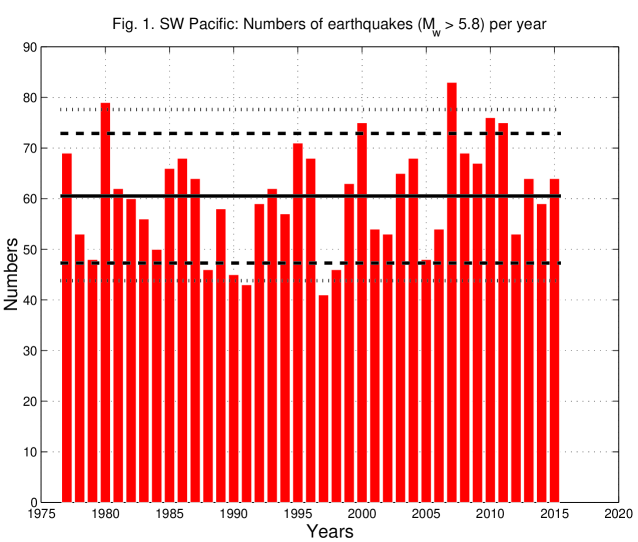
Figure 1: Annual numbers of earthquakes for the GCMT catalog, 1977-2015, $m\geq 5.8$, South-West Pacific. Blue horizontal line shows average annual earthquake number, two blue lines demonstrate 95% confidence areas for the Poisson (dashed lines) and NBD (dotted lines) distributions. Only four annual earthquake numbers are outside of the NBD confidence intervals. For 95% confidence one should expect that about 5% of 39 entries would exceed the limits.

Fig. 1 shows the annual earthquake numbers for the South-West Pacific with 95% levels calculated for the Poisson and NBD laws. Large earthquake numbers usually correspond to the occurrence of a big mainshocks accompanied by an extensive aftershock sequence. Although in four cases the NBD levels are exceeded by observed numbers, this feature is comparable to about 2 cases one should expect for 95% confidence levels. The similar numbers for the Poisson distribution are grossly excessive.

Fig. 2 demonstrates a fit of the empirical annual number distribution for both theoretical curves – Poisson and NBD. The NBD curve once again fits better than the Poisson curve, however the difference between the fits is not large.

Figs. 3–5 demonstrate the approximation of the earthquake numbers in the PDE catalog, subdivided into 1000 intervals of 16.8 days. Earthquake numbers exhibit very large fluctuations with peaks of activity exceeding 600 (see Fig. 3). Neither of the theoretical distributions approximates the observed structure well in Fig. 4; in Fig. 5 the distribution’s heavy tail for the upper seismicity levels is clearly shown, even though the NBD curve is far away from this tail.

These results mean that that NBD is not a good fit for the earthquake number distribution at short time intervals. Unfortunately, as statistical literature (Johnson et al., 2005) demonstrates, there is none of the standard discrete distributions having two degrees of freedom similarly to the NBD. There are many more complicated distributions, such as the generalized Poisson or the generalized NBD, etc., but it is unlikely that their application would be easy and yield reproducible results. Therefore to test earthquake numbers at small time intervals we would need to apply new techniques. One way to test earthquake number distribution would be to use observed distributions for each catalog. These distributions, such as shown in Figs. 2, 4, and 5 would most likely need to be smoothed during the testing.

5 NBD Simulation

To check our results displayed in Tables 2 and 3 we simulate the NBD and process the simulated catalogs similar to real catalogs. To simulate the NBD we use the procedure proposed by Evans et al. (2000, see also Kozubowski & Podgórski, 2009): we first simulate a series of variables distributed according to the geometric distribution (${\bf G:}\ \theta$). The NBD simulation is obtained as a sum of $\tau$ geometric variables

$${\bf NB:}\ \tau,\theta\ \sim\ \sum_{i=1}^{\tau}\,({\bf G:}\ \theta)\,,$$ (5)

i.e., $\tau$ is here the integer, thus is effect we simulate the Pascal distribution, that is a special case of the NBD.

The geometric distribution is simulated by a formula

$${\bf G:}\ \sim[\,\log{\bf R}/\log(1-\theta)\,]-1\,.$$ (6)

where R is the uniform random variate $1.0\geq{\bf R}>0.0$. The result is rounded to the next larger integer (Evans et al. 2000, p. 108).

As simulation input we accept parameter values that are similar to Table 3, line 14: $\theta=0.063$, $\tau=4$. The simulation results reproduce the value of the input parameters, for example, $\hat{\theta}=0.064\pm 0.003$ and $\hat{\tau}=4.06\pm 0.21$. Similarly we obtain $\eta_{n}=0.99\pm 0.03$ and $\psi_{n}=1.48\pm 0.08$ as well as $\eta_{p}=0.129\pm 0.001$ and $\psi_{p}=0.0167\pm 0.0003$.

Fig. 6 displays the scatterplot of skewness ($\eta$) and kurtosis ($\psi$) for the NBD parameters. The values of $\eta$ and $\psi$ correspond well to those of Table 3 (line 14); their standard deviations show that we might expect large random fluctuations of these variables, especially kurtosis: $\eta_{s}=1.012\pm 0.126$ and $\psi_{s}=1.48\pm 0.627$. The values of $\eta_{s}$ and $\psi_{s}$ and especially their standard deviations are different from those shown in previous paragraph for the NBD because the upper values are obtained when the NBD parameters $\theta$ and $\tau$ are first estimated from the simulation series, and their skewness and kurtosis is calculated from these values (as was done in Tables 2 and 3, columns 11 and 12). However, $\eta_{s}$ and $\psi_{s}$ are evaluated directly from the simulated series, thus they are equivalent to $\eta_{o}$ and $\psi_{o}$ in Tables 2 and 3 (columns 9 and 10). However, the input catalog in the simulation case is produced for the NBD whereas the original earthquake catalogs in the Tables are processed. By comparing both results we could see whether the earthquake number distribution is similar in any way to the NBD. Thus the significant difference between $\eta_{s}$ and $\eta_{o}$ as well as between $\psi_{s}$ and $\psi_{o}$ again demonstrates that earthquake number distribution for this catalog temporal subdivision is far from be approximated by the NBD. However, the coefficient of variation for $\eta_{s}$ and $\psi_{s}$ variables shown in Fig. 6 is 12% and 42% respectively, $\eta_{o}$ and $\psi_{o}$ in Tables 2 and 3 are often vary to a much greater degree; for 1000 intervals $\eta_{o}=7.628$ and $\psi_{o}=110.5$ in Table 3. As is seen from Fig. 6 the estimates $\eta_{s}$ and $\psi_{s}$ are strongly correlated, with the correlation coefficient $\rho=0.919$.

To see how simulation results change if longer time intervals are used to subdivide catalogs, we simulate the number distribution for annual intervals. Input parameters are $\theta=0.015$, $\tau=19$ (see Table 3). The results as follows: $\lambda=1252.9\pm 46.7$, $\theta=0.0159\pm 0.0036$, $\tau=20.18\pm 4.50$; $\eta_{s}=0.45\pm 0.43$, $\psi_{s}=0.24\pm 1.32$, and $\rho=0.804$; $\eta_{n}=0.453\pm 0.047$, $\psi_{n}=0.311\pm 0.064$; and $\eta_{p}=0.0283\pm 0.0005$, $\psi_{p}=0.00080\pm 0.00003$. Whereas almost all the values correspond closely to those of line 9 Table 3, $\eta_{o}$ and $\psi_{o}$ are within the random fluctuations of the simulated $\eta_{s}$ and $\psi_{s}$. Fig. 7 illustrates this point.

As a more detailed and accurate statistical test, we compare the difference of two $\eta$ or $\psi$ values with their standard deviations, $\sigma_{\eta}$ and $\sigma_{\psi}$. The ratio

$$z_{\eta}={{\eta_{s}-\eta_{o}}\over{\sigma_{\eta}}}$$ (7)

is distributed for a large number of events ($n>30$) according to a Gaussian distribution with a standard deviation of 1.0. In principle we need to use standard deviations for both items compared, but we have only one deviation for simulated catalogs, thus the test is only approximate. We obtain $z_{\eta}=-2.07$ and $z_{\psi}=-0.84$. Thus for skewness the hypothesis of both items equality is rejected at the significance level slightly higher than 97.5%, whereas for kurtosis the equality of both values is not statistically rejected. Fig. 7 can serve as a confirmation of the above results: only two points of 100 are larger than $\eta_{o}$, whereas eleven simulation points exceed $\psi_{o}$ value.

6 Discussion

We reviewed the theoretical and statistical tools useful in constructing earthquake number test in forecasts of seismic activity as presently practiced by the CSEP. These tools can be used by forecasts practitioners to produce a practical testing algorithm for each particular earthquake catalog and its subdivision.

Generally speaking, the Poisson distribution works reasonably well for yearly samples of magnitude $>6.5$. The NBD works better for smaller event, and especially for shorter time intervals, but neither of the theoretical distributions is adequate for really small events and even shorter intervals.

To see which statistical distribution is the most appropriate for constructing the number test, we study statistical moments of earthquake catalogs and sub-catalogs. Statistical moments are relatively easy to investigate and they are useful in characterizing earthquake occurrence arrangement and seeing which theoretical or empirical laws are most appropriate in approximating them.

We showed that three distributions are useful in number testing: the Poisson, NBD, and the empirical distribution. The Poisson distribution that was traditionally applied for number testing can be only used in restricted cases of the high magnitude threshold. The NBD could be used in most cases for extended time intervals forecasts. However, if forecasts are considered for shorter time intervals such as one month, weeks or days, the fluctuation of earthquake numbers is such that no theoretical distribution can reasonably fit their pattern. Consequently, only empirical distributions are to be used for this purpose.

7   Conclusions

Our results on the forecast testing of earthquake number distribution can be summarized as follows: $\bullet$  1) The Poisson distribution can be used for catalogs of large earthquakes, with magnitude 6.5 and higher. These earthquakes largely occur in a statistically independent manner and their clustering, though present to a minor degree in long catalogs, would not significantly change the result. $\bullet$  2) The NBD can be used for testing distributions in large earthquake catalogs and for long testing periods. $\bullet$  3) No standard statistical distribution appears to fit the event number distribution for short time intervals, of the order of weeks and days. Thus we need to employ empirical distributions obtained for each particular catalog. To be useful such a distribution needs to be properly smoothed.

Table 1: Testing earthquake number distribution

Catalog/Region	n	$<N>$	$\sigma$(N)	$\theta$	$\tau$	$\ell$	$\ell_{0}$	$2\times\Delta\ell$	$\chi^{2}$
CMT NW 77-15	39	36.62	151.47	0.242	11.67	$-9.66$	$-31.64$	43.95	3.37e-11
CMT NW 77-10	34	35.53	80.779	0.440	27.90	$-6.74$	$-11.03$	8.594	0.0034
CMT SW 77-15	39	60.54	106.15	0.570	80.36	$-5.51$	$-6.859$	2.694	0.1007
CMT GL 77-15	39	177.18	737.33	0.240	56.04	$-7.07$	$-15.25$	16.36	5.23e-05
PDE GL 69-14	46	1280.6	88191	0.0145	18.87	$-10.2$	$-252.9$	485.5	0
PDE GL 69-03	35	1147.0	16208	0.0708	87.35	$-7.09$	$-21.84$	29.50	5.59e-08

CMT - Global Centroid-Moment-Tensor catalog: NW - North-West Pacific; SW - South-West Pacific; GL - Global catalog. PDE - Preliminary Determinations of Epicenters catalog. n - number of annual intervals; $<N>$ - average annual number of earthquakes; $\sigma$(N) - standard deviation of N; $\theta$ - clustering parameter of negative binomial distribution (NBD); $\tau$ - parameter of NBD; $\ell$ - NBD log-likelihood; $\ell_{0}$ - Poisson log-likelihood; $\Delta(\ell)=\ell-\ell_{0}$ - log-likelihood difference; $\chi^{2}$ - chi-square value.

Table 2: Values of NBD parameters and skewness and kurtosis for various subdivisions of the 1977-2015 CMT catalogue, $m_{\rm max}=9.15$

#	$m_{t}$	$n$	$N$	$\lambda$	$\sigma$	$\theta$	$\tau$	$\eta_{o}$	$\psi_{o}$	$\eta_{n}$	$\psi_{n}$	$\eta_{p}$	$\psi_{p}$	$\Delta T$
1	2	3	4	5	6	7	8	9	10	11	12	13	14	15
1	7.0	416	39	10.67	10.22	$-$	$-$	0.219	0.070	0.287	0.074	0.306	0.094	365.2
2	6.5	1340	39	34.36	54.33	0.632	59.1	0.086	$-$0.254	0.293	0.120	0.171	0.029	365.2
3	6.0	4359	39	111.8	348.0	0.321	52.9	0.556	$-$0.171	0.280	0.116	0.095	0.009	365.2
4	5.8	6910	39	177.2	742.5	0.239	55.5	0.712	0.017	0.271	0.109	0.075	0.006	365.2
5	5.8	6910	5	1382	17096	0.081	121	0.352	$-$1.319	0.182	0.049	0.027	0.001	2848.8
6	5.8	6910	10	691.0	6857	0.101	77.4	0.762	$-$0.647	0.228	0.078	0.038	0.002	1424.4
7	5.8	6910	20	345.5	2106	0.164	67.8	0.990	0.468	0.244	0.089	0.054	0.003	712.2
8	5.8	6910	39	177.2	742.5	0.239	55.5	0.712	0.017	0.271	0.109	0.075	0.006	365.2
9	5.8	6910	50	138.2	567.0	0.244	44.5	0.543	0.041	0.303	0.137	0.085	0.007	284.9
10	5.8	6910	100	69.10	229.3	0.301	29.8	0.609	0.220	0.372	0.206	0.120	0.015	142.4
11	5.8	6910	200	34.55	91.33	0.378	21.0	1.055	2.376	0.449	0.296	0.170	0.029	71.2
12	5.8	6910	500	13.82	30.26	0.457	11.6	1.566	7.305	0.614	0.550	0.269	0.072	28.5
13	5.8	6910	1000	6.910	13.29	0.520	7.48	1.656	7.508	0.781	0.877	0.380	0.145	14.2
14	5.8	6910	7122	0.970	1.34	0.723	2.53	1.899	7.234	1.524	3.113	1.015	1.031	2.0
15	5.8	6910	14244	0.485	0.62	0.788	1.80	2.364	11.38	1.961	4.956	1.436	2.061	1.0

$m_{t}$ is magnitude threshold value, $n$ is the number of earthquakes, $N$ is the number of time intervals, $\lambda$ - earthquake rate of occurrence; $\sigma$ - standard deviation of earthquake numbers; $\theta$ - clustering parameter of negative binomial distribution (NBD); $\tau$ - parameter of NBD; $\eta_{o}$, $\psi_{o}$ - observed skewness and kurtosis; $\eta_{n}$, $\psi_{n}$ - skewness and kurtosis calculated for NBD; $\eta_{p}$, $\psi_{p}$ - skewness and kurtosis calculated for Poisson distribution; $\Delta T$ – interval duration in days; $m_{\rm max}$ – maximum observed magnitude.

Table 3: Values of NBD parameters and skewness and kurtosis for various subdivisions of the 1969-2014 PDE catalogue, $m_{\rm max}=9.0$

#	$m_{t}$	$n$	$N$	$\lambda$	$\sigma$	$\theta$	$\tau$	$\eta_{o}$	$\psi_{o}$	$\eta_{n}$	$\psi_{n}$	$\eta_{p}$	$\psi_{p}$	$\Delta T$
1	2	3	4	5	6	7	8	9	10	11	12	13	14	15
1	7.0	560	46	12.17	14.10	0.863	76.9	0.517	0.753	0.351	0.149	0.287	0.0821	365.2
2	6.5	1635	46	35.54	58.12	0.612	56.0	0.212	0.286	0.298	0.124	0.168	0.0281	365.2
3	6.0	4826	46	104.9	526.6	0.199	26.1	0.763	0.273	0.394	0.232	0.098	0.0095	365.2
4	5.5	16651	46	362.0	6369	0.057	21.8	0.893	0.230	0.428	0.275	0.053	0.0028	365.2
5	5.0	58909	46	1281	88191	0.015	18.9	1.386	1.436	0.460	0.318	0.028	0.0008	365.2
6	5.0	58909	5	11781	387e4	0.003	35.9	1.452	0.187	0.334	0.167	0.009	0.0001	3360
7	5.0	58909	10	5891	121e4	0.005	28.6	1.030	0.030	0.374	0.210	0.013	0.0002	1680
8	5.0	58909	20	2945	400e3	0.007	21.8	1.088	$-$0.069	0.428	0.275	0.018	0.0003	840.0
9	5.0	58909	46	1281	88191	0.015	18.9	1.386	1.436	0.460	0.318	0.028	0.0008	365.2
10	5.0	58909	50	1178	88856	0.013	15.8	1.712	2.902	0.503	0.379	0.029	0.0009	336.0
11	5.0	58909	100	589.1	27994	0.021	12.7	2.375	8.006	0.562	0.474	0.041	0.0017	168.0
12	5.0	58909	200	294.5	8559	0.034	10.5	2.697	12.34	0.617	0.572	0.058	0.0034	84.0
13	5.0	58909	500	117.8	2339	0.050	6.25	4.756	41.18	0.800	0.960	0.092	0.0085	33.6
14	5.0	58909	1000	58.91	942.4	0.063	3.92	7.628	110.5	1.010	1.529	0.130	0.0170	16.8
15	5.0	58909	8400	7.013	48.92	0.143	1.17	19.64	823.0	1.852	5.133	0.378	0.1426	2.0
16	5.0	58909	16801	3.506	17.94	0.196	0.85	23.18	1224	2.180	7.100	0.534	0.2852	1.0

$m_{t}$ is magnitude threshold value, $n$ is the number of earthquakes, $N$ is the number of time intervals, $\lambda$ - earthquake rate of occurrence; $\sigma$ - standard deviation of earthquake numbers; $\theta$ - clustering parameter of negative binomial distribution (NBD); $\tau$ - parameter of NBD; $\eta_{o}$, $\psi_{o}$ - observed skewness and kurtosis; $\eta_{n}$, $\psi_{n}$ - skewness and kurtosis calculated for NBD; $\eta_{p}$, $\psi_{p}$ - skewness and kurtosis calculated for Poisson distribution; $\Delta T$ – interval duration in days; $m_{\rm max}$ – maximum observed magnitude.

Acknowledgments

I am grateful to Peter Bird of UCLA for useful discussions. The author appreciates partial support from the National Science Foundation through grant EAR-1045876, as well as from the Southern California Earthquake Center (SCEC). This research was supported by the Southern California Earthquake Center. SCEC is funded by NSF Cooperative Agreement EAR-1033462 & USGS Cooperative Agreement G12AC20038. Publication 7071, SCEC.

References

Bird, P., D. D. Jackson, Y. Y. Kagan, C. Kreemer, and R. S. Stein, 2015. GEAR1: a Global Earthquake Activity Rate model constructed from geodetic strain rates and smoothed seismicity, Bull. Seismol. Soc. Amer., 105(5), 2538-2554, doi:10.1785/0120150058, (plus electronic supplement).

Bowman, K. O., Shenton, L. R. (1986). Moment (${\sqrt{b}_{1}},b_{2}$) Techniques. In: D’Augustino, R. B., Stephens, M. A., eds. Goodness of Fit Techniques. Statistics: Textbooks and Monographs. Vol. 68. New York: Marcel Dekker, pp. 279-327.

D’Augustino, R. B., and M. A. Stephens (1986). Goodness-of-fit techniques, in Statistics: Textbooks and Monographs, Vol. 68, Marcel Dekker, New York, 560 pp.

Ekström, G., M. Nettles & A.M. Dziewonski, 2012. The global CMT project 2004-2010: Centroid-moment tensors for 13,017 earthquakes, Phys. Earth Planet. Inter., 200-201, 1-9. 10.1016/j.pepi.2012.04.002

Evans, M., N. Hastings, and B. Peacock, 2000. Statistical Distributions, 3rd ed., New York, J. Wiley, 221 pp.

Feller, W., 1968. An Introduction to Probability Theory and its Applications, 1, 3-rd ed., J. Wiley, New York, 509 pp.

Johnson, N. L., A. W. Kemp, and S. Kotz, 2005. Univariate Discrete Distributions, 3rd ed., Wiley, Hoboken, New Jersey, 646 pp.

Kagan, Y. Y., 2003. Accuracy of modern global earthquake catalogs, Phys. Earth Planet. Inter. (PEPI), 135(2-3), 173-209.

Kagan, Y. Y., 2010. Statistical distributions of earthquake numbers: consequence of branching process, Geophys. J. Int., 180(3), 1313-1328. doi: 10.1111/j.1365-246X.2009.04487.x

Kagan, Y. Y., 2014. EARTHQUAKES: Models, Statistics, Testable Forecasts, Hoboken, NJ, John Wiley & Sons, 306 pp, ISBN: 978-1118637913.

Kozubowski, T. J., and K. Podgórski, 2009. Distributional properties of the negative binomial Lévy process, Probability and Mathematical Statistics, 29(1), 43-71.

Li, G., and A. Papadopoulos, 2002. A note on goodness of fit test using moments, Statistica, 62(1), 71-86.

Stephens, M. A., 1986. Tests based on EDF statistics, in: Goodness-of-Fit Techniques, Statistics: Textbooks and Monographs, Vol. 68, edited by: D’Augustino, R. B. and Stephens, M. A., Marcel Dekker, New York, 97-194, 1986.

U.S. Geological Survey, Preliminary Determinations of Epicenters (PDE), 2008. U.S. Dep. of Inter., Natl. Earthquake Inf. Cent. http://neic.usgs.gov/neis/epic/code_catalog.html

Wilks, S. S., 1962. Mathematical Statistics, John Wiley, New York, 644 pp.

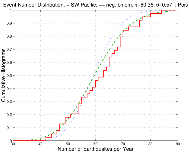
Figure 2:

Cumulative distribution of yearly earthquake numbers for the GCMT catalog, 1977-2015, $m\geq 5.8$, South-West Pacific. The step-function shows the observed distribution, the dashed curve is the theoretical Poisson distribution for $\lambda=60.54$ and the dashed curve is the fitted negative-binomial curve for $\theta=0.570$ and $\tau=80.36$. As expected from Table 1 results the negative-binomial curve has a better fit than the Poisson curve, though the difference is not large.

Figure 3: Numbers of earthquakes for the PDE catalog, 1969-2014, $m\geq 5.0$, subdivided into 1000 intervals (duration 16.8 days, see Table 3). Blue horizontal line shows average annual earthquake number, two blue lines demonstrate 95% confidence areas for the Poisson (dashed lines) and NBD (dotted lines) distributions. Many of the annual earthquake numbers are outside of the NBD confidence intervals, thus the NBD poorly approximating the number distribution.

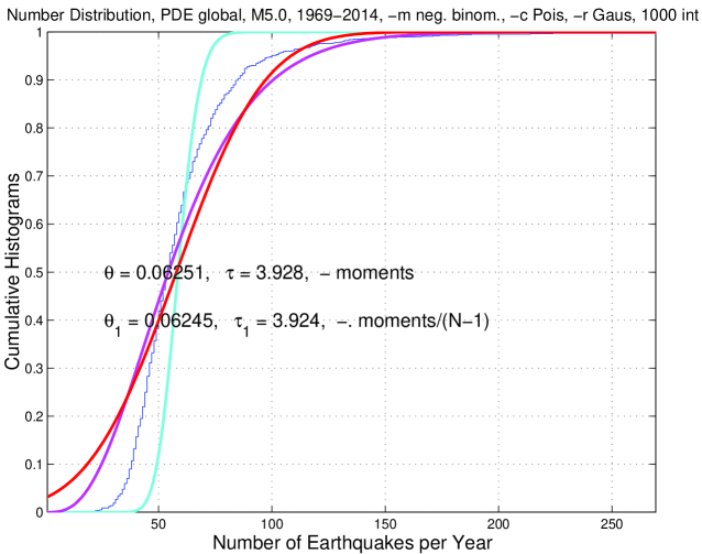
Figure 4:

Blue curve is cumulative distribution of yearly global earthquake numbers for the PDE catalog, 1969-2014, $m\geq 5.0$. The step-function shows the observed distribution, the red curve is the Gaussian distribution, the cyan curve is the theoretical Poisson distribution for $\lambda=58.9$ and the magenta solid curve is the fitted negative-binomial curve for $\theta=0.063$ and $\tau=3.93$. The negative-binomial curve has a better fit than the Poisson curve.

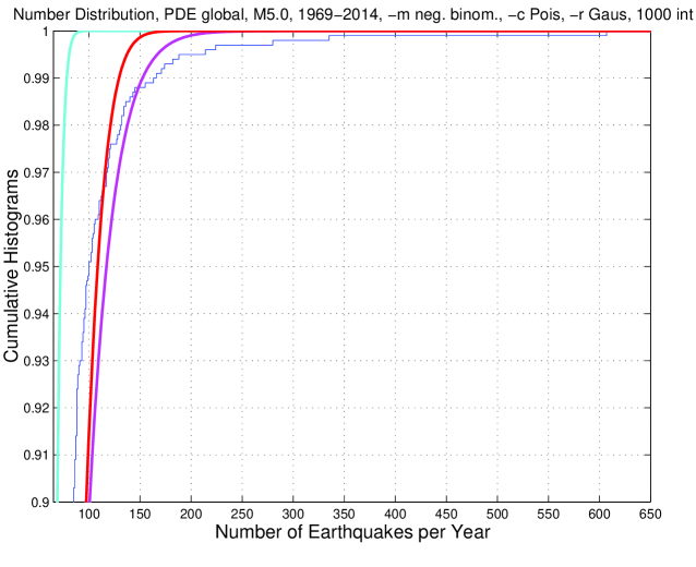
Figure 5:

Same as Fig. 4 but only the upper part of distribution curves is displayed. Kurtosis values for curves, from left to right (see Table 3): $\psi_{p}=0.02$, $\psi_{g}=0$, $\psi_{n}=1.53$, $\psi_{o}=110.5$.

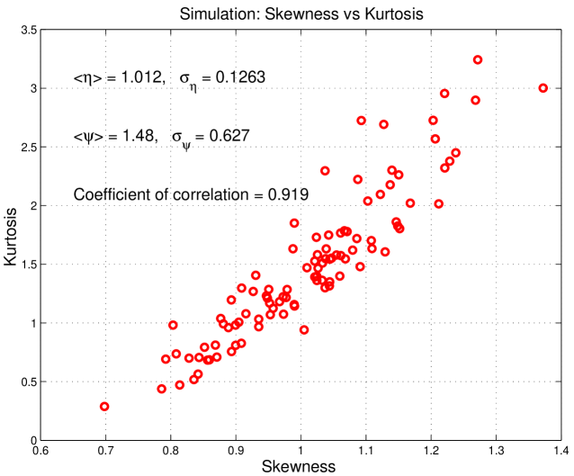
Figure 6:

Scatterplot of skewness ($\eta$) and kurtosis ($\psi$) for simulated NBD for 1000 intervals catalog subdivision.

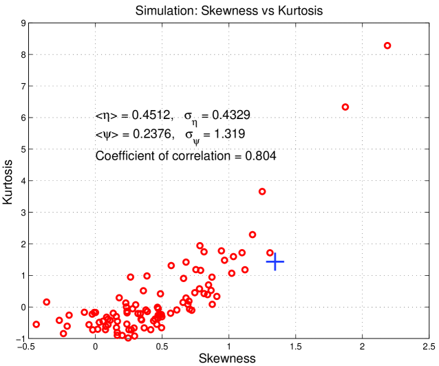
Figure 7:

Scatterplot of skewness ($\eta$) and kurtosis ($\psi$) for simulated NBD for annual interval catalog subdivision. Large blue cross shows skewness ($\eta_{o}$) and kurtosis ($\psi_{o}$) for the annual subdivision of the PDE catalog (see Table 3).