One- and two-dimensional solitons in $\mathcal{PT}$-symmetric systems emulating the spin-orbit coupling

Abstract

We introduce a two-dimensional (2D) system, which can be implemented in dual-core planar optical couplers with the Kerr nonlinearity in its cores, making it possible to blend effects of the $\mathcal{PT}$ symmetry, represented by balanced linear gain and loss in the two cores, and spin-orbit coupling (SOC), emulated by a spatially biased coupling between the cores. Families of 1D and 2D solitons and their stability boundaries are identified. In the 1D setting, the SOC leads, at first, to shrinkage of the stability area for $\mathcal{PT}$-symmetric solitons, which is followed by its rapid expansion. 2D solitons have their stability region too, in spite of the simultaneous action of two major destabilizing factors, viz., the collapse driven by the Kerr nonlinearity and a trend towards spontaneous breakup of the gain-loss balance. In the limit of the SOC terms dominating over the intrinsic diffraction, the 1D system gives rise to a new model for gap solitons, which admits exact analytical solutions.

Keywords: optical coupler; Kerr nonlinearity; gain and loss; collapse; symmetry breaking; soliton stability; spatiotemporal solitons; gap solitons

I Introduction

The recent progress in the experimental and theoretical work with engineered optical media has made it possible to emulate, by means of the optical-beam propagation, a wide range of physical effects which were originally predicted or experimentally discovered in other areas of physics. In many cases, the optical emulation offers a possibility to study the effect in question in a pure form, which is often too difficult in the original setting. In other cases, specially designed optical configurations open a way to demonstrate realizations of the effects in forms which are impossible in the source systems. Belonging to this class of optically emulated phenomena are the parity-time ($\mathcal{PT}$) symmetry Bender , based on the paraxial beam propagation in optical media with symmetrically placed gain and loss elements, as predicted theoretically PT-optics and realized experimentally PT-optics-exp ; Anderson localization in random photonic media Anderson ; and the photonic emulation of topological insulators opt-top-insulator and graphene opt-graphene . A recent addition to this topic is a proposal to implement the mechanism of the spin-orbit coupling (SOC), previously elaborated in terms of Bose-Einstein condensates (BECs) SOC , in dual-core optical waveguides opt-SOC-2D ; opt-SOC-1D .

Basic schemes of “grafting” new physical effects to optics make use of linear beam-propagation regimes. However, the ubiquitous Kerr nonlinearity of optical materials, as well as other types of the optical nonlinear response, suggest one to consider implementation of the new effects in a nonlinear form. A well-known example is provided by $\mathcal{PT}$-symmetric solitons, which have been studied in detail theoretically PT-sol-theory and created in the experiment PT-sol-exp . The optical emulation of the SOC was also developed in the context of the nonlinear propagation and formation of solitons opt-SOC-2D .

As a further development in these directions, it may be interesting to design optical settings which combine the above-mentioned effects, that would be difficult to achieve in their original realizations. The objective of the present work is to elaborate one- and two-dimensional (1D and 2D) optical systems, based on dual-core waveguides, which make it possible to blend the SOC and $\mathcal{PT}$-symmetry mechanisms. The use of couplers for this purpose is natural, as they provide photonic platforms for the emulation of both the SOC and $\mathcal{PT}$ symmetry in 1D opt-SOC-1D ; Radik and 2D opt-SOC-2D ; Gena geometries alike. As an additional result of the analysis, a new 1D conservative model for two-component gap solitons is produced, which admits exact solutions, and demonstrates a nontrivial internal stability boundary in the soliton family. New dynamical features are revealed by the analysis of the combined models, such as a nonmonotonous dependence of the stability area of 1D $\mathcal{PT}$-symmetric solitons on the SOC strength, $\delta$: the area originally shrinks but then strongly expands with the increase of $\delta$. Another noteworthy finding is that the SOC terms stabilize 2D $\mathcal{PT}$-symmetric solitons under the action of the cubic self-attraction, in spite of the simultaneous presence of two mechanisms driving the catastrophic instability in the 2D system: the possibility of the breakup of the $\mathcal{PT}$ symmetry, i.e., failure of the gain-loss balance PT-optics ; PT-sol-theory , and the onset of the critical collapse induced by the Kerr nonlinearity collapse (the latter may also take place in the presence of SOC Bilbao ). The latter result implies extension of the SOC-induced stabilization of 2D solitons (semi-vortices and mixed modes) in the free space with the cubic self-attraction, that was demonstrated recently we .

The paper is organized as follows. The basic model is introduced in Section II. Results for 1D solitons and their stability are collected in Section III. The new 1D model for gap solitons and its $\mathcal{PT}$-symmetric version are presented in Section IV. Results for 2D solitons are reported in Section V, and the paper is concluded by Section VI.

II The model

The starting point is a model for the dual-core planar optical waveguide which governs the spatiotemporal evolution of local amplitudes of the electromagnetic waves in two cores, $U_{1}\left(x,t,z\right)$ and $U_{2}\left(x,t,z\right)$, under the action of the anomalous group-velocity dispersion (GVD) and Kerr nonlinearity:

$$i\left(U_{1}\right)_{z}+\frac{1}{2}\left[\left(U_{1}\right)_{tt}+\left(U_{1}\right)_{xx}\right]+U_{2}+\left|U_{1}\right|^{2}U_{1} = 0,$$ (1)

$$i\left(U_{2}\right)_{z}+\frac{1}{2}\left[\left(U_{2}\right)_{tt}+\left(U_{2}\right)_{xx}\right]+U_{1}+\left|U_{2}\right|^{2}U_{2} = 0.$$ (2)

In these coupled 2D nonlinear Schrödinger equations (NLSEs) $z$ is the propagation distance, $x$ the transverse coordinate, $t$ the reduced temporal variable, the second $x$ derivatives account for the paraxial diffraction, while the coupling coefficient, together with the GVD and Kerr coefficients, are scaled to be $1$. The 1D reduction of Eqs. (1) and (2) amounts to the commonly known 1D model for dual-core optical fibers or the spatial propagation in the twin-core planar waveguides coupler .

By itself, the system of Eqs. (1) and (2) gives rise solely to unstable 2D solitons, due to the occurrence of the collapse in the same setting. The stabilization of the spatiotemporal solitons against the collapse may be provided by the optical counterpart of the SOC, which amounts to taking into account the temporal dispersion of the coupling coefficient opt-SOC-2D , represented by terms $\delta\left(U_{2}\right)_{t}$ and $\delta\left(U_{1}\right)_{t}$ to be added to Eqs. (1) and (2), respectively, with a real dispersion coefficient $\delta$ Chiang . The accordingly modified coupled equations, which also include the balanced gain and loss terms, with real coefficient $\Gamma>0$ Radik , that introduce the $\mathcal{PT}$ symmetry, take the form of

$$i\left(U_{1}\right)_{z}+\frac{1}{2}\left[\left(U_{1}\right)_{tt}+\left(U_{1}\right)_{xx}\right]+i\delta(U_{2})_{t}+U_{2}+\left|U_{1}\right|^{2}U_{1} = i\Gamma U_{1},$$ (3)

$$i\left(U_{2}\right)_{z}+\frac{1}{2}\left[\left(U_{2}\right)_{tt}+\left(U_{2}\right)_{xx}\right]+i\delta(U_{1})_{t}+U_{1}+\left|U_{2}\right|^{2}U_{2} = -i\Gamma U_{2}.$$ (4)

All the ingredients of the present system, including the separated gain and loss PT-optics-exp , can be realized experimentally in optics. Nevertheless, the model based on Eqs. (3) and (4) turns out to be irrelevant, because the linearized version of the equations for excitations, in the usual form of $U_{1,2}\sim\exp\left(ikz-i\omega t+iqx\right)$,  gives rise to an unstable dispersion relation between the propagation constant, $k$, real temporal frequency, $\omega$, and real transverse wavenumber, $k$:

$$\left(k+\frac{1}{2}\omega^{2}+\frac{1}{2}q^{2}\right)^{2}=-\Gamma^{2}+\left(1+\delta\cdot\omega\right)^{2}.$$ (5)

Indeed, it follows from Eq. (5) that, in the presence of the gain and loss, the zero solution is unstable, which is accounted for by an imaginary part of $k$, against perturbations with $\left(1+\delta\cdot\omega\right)^{2}<\Gamma^{2}$. In other words, the $\mathcal{PT}$ symmetry is always broken by the SOC terms in this system, while it gives rise to stable 2D solutions at $\Gamma=0$ opt-SOC-2D .

A system which maintains the $\mathcal{PT}$ symmetry in the presence of the SOC is based on the following coupled NLSEs:

$$i\left(U_{1}\right)_{z}+\frac{1}{2}\left[\left(U_{1}\right)_{tt}+\left(U_{1}\right)_{xx}\right]-\delta\left(U_{2}\right)_{x}+U_{2}+\left|U_{1}\right|^{2}U_{1} = i\Gamma U_{1},$$ (6)

$$i\left(U_{2}\right)_{z}+\frac{1}{2}\left[\left(U_{2}\right)_{tt}+\left(U_{2}\right)_{xx}\right]+\delta\left(U_{1}\right)_{x}+U_{1}+\left|U_{2}\right|^{2}U_{2} = -i\Gamma U_{2}.$$ (7)

This is a model of a planar coupler, in which the temporal dispersion of the coupling coefficient is disregarded, while terms $\mp\delta\left(U_{2,1}\right)_{x}$ account for “skewness” of the coupling in the transverse direction, assuming that the layer between the guiding cores has an oblique structure. Roughly speaking, the latter means that light tunnels between point $x$ in the first (second) core and point $x+\delta$ (respectively, $x-\delta$) in the mate core. The dispersion relation for the linearized version of Eqs. (6) and (7) is

$$\left(k+\frac{1}{2}\omega^{2}+\frac{1}{2}q^{2}\right)^{2}=1-\Gamma^{2}+\left(\delta\cdot q\right)^{2}.$$ (8)

Unlike Eq. (5), it demonstrates that the $\mathcal{PT}$ symmetry holds at $\Gamma\leq 1$ (in fact, under the condition that the gain-loss coefficient is smaller than the inter-core coupling constant, which is scaled to be $1$).

The system may produce solitons in its bandgap, i.e., at values of the propagation constant, $k$, which cannot be obtained from Eq. (8). Simple analysis demonstrates that the dispersion relation (8) gives rise to a semi-infinite bandgap, in which solitons are expected to exist:

$$k>\left\{\begin{array}[]{c}\frac{1}{2}\left[\delta^{2}+\left(1-\Gamma^{2}\right)\delta^{-2}\right],~{}\mathrm{at}~{}~{}\delta^{2}>\sqrt{1-\Gamma^{2}},\\ \sqrt{1-\Gamma^{2}},~{}\mathrm{at}~{}~{}\delta^{2}<\sqrt{1-\Gamma^{2}}.\end{array}\right.$$ (9)

III Solitons in the 1D system

A family of stationary soliton solutions of the 1D version of Eqs. (6) and (7), in which the temporal dependence is dropped, are looked for as

$$U_{1,2}(x,z)=\exp\left(ikz\right)u_{1,2}(x),$$ (10)

with complex functions $u_{1,2}(x)$ satisfying equations

$$\frac{1}{2}u_{1}^{\prime\prime}-\delta u_{2}^{\prime}+u_{2}+\left|u_{1}\right|^{2}u_{1} = \left(k+i\Gamma\right)u_{1},$$ (11)

$$\frac{1}{2}u_{2}^{\prime\prime}+\delta u_{1}^{\prime}+u_{1}+\left|u_{2}\right|^{2}u_{2} = \left(k-i\Gamma\right)u_{2},$$ (12)

with the prime standing for $d/dx$. The $\mathcal{PT}$ symmetry amounts to the cross-symmetry constraint for the two components, which all the soliton solutions obey:

$$u_{1}(-x)=u_{2}^{\ast}(x)$$ (13)

(the asterisk stands for the complex conjugation). The solutions are characterized by their norm, i.e., the total power, in terms of the underlying optics model:

$$N=\int_{-\infty}^{+\infty}\left[|u_{1}(x)|^{2}+|u_{2}(x)|^{2}\right]dx.$$ (14)

In the absence of the SOC terms ($\delta=0$), exact $\mathcal{PT}$-symmetric soliton solutions to Eqs. (11) and (12) are well known Radik ,

$$u_{2}(x)=e^{i\phi}\left(\sqrt{1-\Gamma^{2}}+i\Gamma\right)u_{1}(x),~{}$$

$$u_{1}(x)=e^{i\phi}\sqrt{2\left(k-\sqrt{1-\Gamma^{2}}\right)}\mathrm{sech}\left(\sqrt{2\left(k-\sqrt{1-\Gamma^{2}}\right)}x\right),$$ (15)

where $\phi$ is a constant phase. The exact stability condition for these solutions is known too Radik . Combined with the obvious existence condition, $k>\sqrt{1-\Gamma^{2}}$, it produces the following interval filled by the stable $\mathcal{PT}$-symmetric solitons at $\delta=0$ (in the absence of the SOC terms): $\sqrt{1-\Gamma^{2}}<k<\left(5/3\right)\sqrt{1-\Gamma^{2}}$. It is more relevant to write this in terms of the norm of soliton (15), $N\left(\delta=0\right)=4\sqrt{2\left(k-\sqrt{1-\Gamma^{2}}\right)}$:

$$0<N<\left(8/\sqrt{3}\right)\left(1-\Gamma^{2}\right)^{1/4}\equiv N_{\mathrm{c}}\left(\delta=0\right).$$ (16)

In the presence of the SOC ($\delta>0$), we have built stationary localized solutions of the system by means of the well-known imaginary-time-integration method Tosi . Figures 1(a), (b), and (c) show typical profiles of the stable solutions for $|u_{1}(x)|$ and $|u_{2}(x)|$, obtained at particular values of the SOC and $\mathcal{PT}$ parameters, $\delta$ and $\Gamma$, specified in the caption to Fig. 1. Selected for the comparison in this figure are the solitons which all have equal norms, $N=3$.

Figure 1: Profiles of components $|u_{1}(x)|$ and $|u_{2}(x)|$ (solid and dashed lines, respectively ) in the 1D solitons at the following values of the SOC and gain-loss coefficients: (a) $\delta=0.5$, $\Gamma=0.3$, (b) $\delta=2$, $\Gamma=0.3$, and (c) $\delta=2$, $\Gamma=0.8.$ All the solitons have the same total norm, $N=3$. (d) Distance $\Delta x$ between peaks of the two components vs. $\delta$ at $\Gamma=0.3$.

A notable SOC effect is the splitting between peaks of the two components. A simple perturbative analysis of Eqs. (11) and (12) demonstrates that, for small $\delta$, the distance between the peaks is

$$\Delta x=\delta.$$ (17)

Figure 1(d) shows the numerically obtained distance $\Delta x$ as a function of $\delta$ for $\Gamma=0.3$. Thus, relation (17) is virtually exact at $\delta\leq 0.4$.

It is worthy to note that the profiles of $\left|u_{1}(x)\right|$ and $\left|u_{2}(x)\right|$ are nearly identical for different values of the gain-loss coefficient, $\Gamma=0.3$ and $0.8$, with the same $\delta=2$, in Figs. 1(b,c). This observation is in qualitative agreement with the fact that, for given $N$, the profiles of exact solitons (15) do not depend on $\Gamma$ either.

An obvious effect of the increase of $\delta$ is a transition from the smooth soliton profile to a multi-lobe structure, as seen from the comparison of panels (a) and (b,c) in Fig. 1. This fact can be explained by the inversion of the dispersion relation (8), to express $q$ in terms of $k$, at $\omega=0$. The result of a simple algebra is that, precisely at $k>\sqrt{1-\Gamma^{2}}$, i.e., when the exact soliton (15) exists for $\delta=0$, wavenumber $q$ becomes complex, which implies the wavy profile of the soliton’s tails, for

$$\delta^{2}>k-\sqrt{k^{2}-\left(1-\Gamma^{2}\right)}.$$ (18)

The numerical results demonstrate that the transition occurs at $\delta\approx 0.6$ for $\Gamma=0.3$, and at $\delta\approx 0.7$ for $\Gamma=0.8$, which is consistent with Eq. (18) in which numerically obtained values of $k$ are substituted.

The stable soliton family is further characterized by Fig. 2(a), which shows the largest value of the field $|u_{1}(x)|$ as a function of $N$, for $\delta=2$ and $\Gamma=3$. Naturally, $|u_{1}(x=0)|$ increases monotonously with $N$, up to a critical value, $N_{\mathrm{c}}$, at which the destabilization of the solitons happens via the breakup of the $\mathcal{PT}$ symmetry (the solitons exist at $N>N_{\mathrm{c}}$ as unstable solutions, which cannot be found by means of the imaginary-integration method). In the conservative system with $\Gamma=0$, stable asymmetric solitons, with $u_{1}(x)\neq u_{2}(-x)$, may exist at $N>N_{\mathrm{c}}$, but in the presence of $\Gamma>0$ this is impossible, as asymmetric solitons would not maintain the balance between the gain and loss. Figure 2(d) shows an example of a stable asymmetric solution found at $\Gamma=0$ for $N=5$ and $\delta=2$

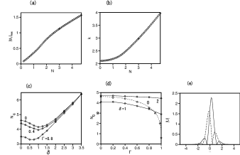
Figure 2: (a) Maximum value of $|U_{1}|$ of stable 1D solitons, as a function of $N$ for $\delta=2$ and $\Gamma=0.3$. (b) The critical norm, $N_{\mathrm{c}}$ (above which stable 1D solitons do not exist), as a function of the SOC strength, $\delta$, for values of the gain-loss coefficient $\Gamma=0$, $0.4$, and $0.8$. (c) The critical norm versus $\Gamma$, for $\delta=0$, $1$, and $2$. (d) An example of a stable symmetric solution found in the conservative model, with $\Gamma=0$, for $N=5$ and $\delta=2$.

In fact, $N_{\mathrm{c}}$ is the most important characteristic of the soliton families. It is shown, as a function of the SOC strength, $\delta$, for fixed $\Gamma=0$, $0.4$, and $0.8$, in Fig. 2(b). In particular, $N_{\mathrm{c}}$ is given by the exact expression (16) for $\delta=0.$ The initial decrease of $N_{\mathrm{c}}$, which is observed in Fig. 2(b) at relatively small $\delta$, can be easily understood: as shown by Eq. (17), the two components get separated by distance $\Delta x\approx\delta$, hence the effective linear coupling between the components weakens with the increase of $\delta$, making a smaller strength of the Kerr nonlinearity (measured by the norm) sufficient to initiate the symmetry breaking between the two components. Obviously, this effect should scale as $\delta^{2}$, which is consistent with Fig. 2(b) at $\delta$ small enough. However, a nontrivial finding is that, at $\delta$ exceeding values corresponding to the minimum of $N_{\mathrm{c}}$ in Fig. 2(b), $N_{\mathrm{c}}$ features rapid increase with $\delta$, which becomes asymptotically linear at large values of $\delta$. This property is explained in the next section which addresses the limit form of system (6), (7) with the SOC terms dominating over the paraxial diffraction.

Further, Fig. 2(c) shows $N_{\mathrm{c}}$ as a function of $\Gamma$ for fixed SOC strengths, $\delta=0$, $1$, and $2$, the dashed curve representing the exact result given by Eq. (15) for $\delta=0$. This figure shows too that the SOC terms tend to essentially expand the stability area for the $\mathcal{PT}$-symmetric solitons, by increasing $N_{\mathrm{c}}$. However, even if $N_{\mathrm{c}}$ keeps a nonzero value up to $\Gamma=1$ at $\delta>0$, there is no stability region at $\Gamma>1$, as the zero solution (the background of the solitons) is unstable in the latter case, as follows from Eq. (8).

IV The limit case of negligible intrinsic diffraction

The results displayed above in Fig. 2(b) for large $\delta$ suggest to consider the limit case of the system in which the SOC terms dominate over the paraxial diffraction. Dropping the second derivatives in the 1D version of Eqs. (3) and (4), one thus arrives at the simplified system,

$$i\left(U_{1}\right)_{z}-\delta\left(U_{2}\right)_{x}+U_{2}+\left|U_{1}\right|^{2}U_{1} = i\Gamma U_{1},$$ (19)

$$i\left(U_{2}\right)_{z}+\delta\left(U_{1}\right)_{x}+U_{1}+\left|U_{2}\right|^{2}U_{2} = -i\Gamma U_{2}.$$ (20)

whose dispersion relation is

$$k^{2}=1-\Gamma^{2}+\left(\delta\cdot q\right)^{2},$$ (21)

cf. Eq. (15). It gives rise to a finite bandgap, $k^{2}<$ $1-\Gamma^{2}$ [unlike the semi-infinite bandgap given by Eq. (9)], hence the corresponding localized states may be considered as gap solitons. Actually, the system of Eqs. (19) and (20) with $\Gamma=0$ is a new conservative model generating gap solitons, therefore it makes sense to consider its solutions, along with its $\mathcal{PT}$-symmetric version, corresponding to $0<\Gamma<1$. An essential difference from the standard gap solitons generated by the Bragg-grating model Bragg is the separation between peaks of the two components, and, on the other hand, gap-soliton solutions are real in the present model.

Looking for stationary solutions to Eqs. (19) and (20) as per Eq. (10), in the absence of the gain and loss, $\Gamma=0$, functions $u_{1}(x)$ and $u_{2}(x)$ satisfy a system of real equations

$$-ku_{1}-\delta u_{2}^{\prime}+u_{2}+u_{1}^{3} = 0,$$ (22)

$$-ku_{2}+\delta u_{1}^{\prime}+u_{1}+u_{2}^{3} = 0,$$ (23)

whose solutions obey the cross-symmetry constraint, cf. Eq. (13): $u_{1}(-x)=u_{2}(x).$ In fact, $\delta$ may be easily absorbed into rescaled coordinate $x$, therefore numerical results are presented below for $\delta=1$. The total norm (14), defined according to the original coordinate, scales as $\delta$, which explains the asymptotically linear $N_{\mathrm{c}}(\delta)$ dependence in Fig. 2(b).

It is possible to find exact soliton solutions to Eqs. (22) and (23), noting that the evolution of $u_{1}$ and $u_{2}$ along $x$ conserves the corresponding formal Hamiltonian:

$$h=\frac{k}{2}\left(u_{1}^{2}+u_{2}^{2}\right)-u_{1}u_{2}-\frac{1}{4}\left(u_{1}^{2}+u_{2}^{2}\right)^{2}+\frac{1}{2}u_{1}^{2}u_{2}^{2}.$$ (24)

Next, it is convenient to represent solutions in the “polar” form,

$$u_{1}(x)=u(x)\cos\left(\theta(x)\right),~{}u_{2}(x)=u(x)\sin\left(\theta(x)\right)$$ (25)

For soliton solutions which vanish at $x\rightarrow\pm\infty$, one should set $h=0$, hence Eq. (24) makes it possible to eliminate $u^{2}$ in favor of $\theta$, after substituting expressions (25):

$$u^{2}=4\frac{k-\sin(2\theta)}{2-\sin^{2}(2\theta)},$$ (26)

Finally, combining two equations (22) and (23) and Eq. (26), it is easy to derive a single equation for $\theta(x)$:

$$\delta\frac{d\theta}{dx}=k-\sin(2\theta).$$ (27)

A solution to Eq. (27), which generates a soliton after the substitution in Eq. (26), exists for $k^{2}<1$:

$$\theta=-\frac{\pi}{4}+\arctan\left[\frac{1+k}{\sqrt{1-k^{2}}}\tanh\left(\frac{\sqrt{1-k^{2}}}{\delta}x\right)\right].$$ (28)

The total norm of the solitons calculated as per Eqs. (14) and (25)-(28), can be written as

$$N(k)=2\sqrt{2}\delta\left\{\begin{array}[]{c}-\arctan\left(\sqrt{2\left(1-k^{2}\right)}/k\right),~{}-1<k<0,\\ \left[\pi-\arctan\left(\sqrt{2\left(1-k^{2}\right)}/k\right)\right],~{}0<k<1.\end{array}\right.$$ (29)

Thus, with the increase of $k$ from $-1$ to $+1$, $N(k)$ monotonously grows from $N(k=-1)=0$ to $N(k=+1)=2\sqrt{2}\pi\delta$. The analytical solution makes it possible to find the distance between peaks of the two components, cf. Eq. (17). In the general case, the analytical expression for $\Delta x$ is cumbersome. It takes a relatively simple form for $k=0$, which corresponds to a stable gap soliton (see below):

$$\Delta x(k=0)=2\delta\mathrm{Artanh}\left(\frac{1-3^{1/4}\left(\sqrt{3}-1\right)}{2-\sqrt{3}}\right)\approx 0.275~{}\delta.$$ (30)

Figure 3(a) displays an example of the exact solution for $k=-0.5$ and $\delta=1$, whose total norm is $N=3.35$, in agreement with Eq. (29). Further, Fig. 3(b) shows a result of the test of the stability of this gap soliton, produced by direct simulations of Eqs. (19) and (20) with $\Gamma=0$ and small random perturbations added to the initial conditions. Figure 3(b) clearly shows that the gap soliton is stable.

Figure 3(c) displays another example of the exact soliton,for $k=0.6$ and $\delta=1$, with the total norm $N=5.82$, which also agrees with Eq. (29). In this case, the simulations, the result of which is shown in the top plot of Fig. 3(d) at $z=800$, demonstrate weak instability of the soliton, which leads to generation of an undulating tail. The simulations for other values of $k$, that are displayed too in Fig. 3(d), suggest that the intrinsic boundary between stable and unstable gap solitons is located at $k\approx 0.5$, cf. a qualitatively similar results for the gap solitons in the Bragg-grating model Bragg-stability .

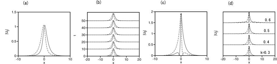
Figure 3: (a) The exact solution for $|u_{1}(x)|$ and $|u_{2}(x)|$ (solid and dashed lines), given by Eqs. (25)-(29) for $k=-0.5$ and $\delta=1$. (b) The perturbed evolution of component $\left|U_{1}(x,t)\right|$ of the same gap soliton, corroborating its stability. (c) The exact solution for $k=0.6$ and $\delta=1$. (d) Snapshots produced by the simulations of the perturbed evolution of the gap solitons with $k=0.3,0.4,0.5$, and $0.6$, at $z=800$. The results reveal a boundary between stable and unstable solitons at $k\approx 0.5$.

The $\mathcal{PT}$-symmetric version of Eqs. (19) and (20) with $\Gamma>0$ was solved numerically, which also produced solitons. Two examples, for $\delta=1$ and $\Gamma=0.5$, but different propagation constants, $k=-0.5$ and $k=0.6$, with the norms, respectively, $N=3.20$ and $6.31$, are displayed in Figs. 4(a) and (c). Simulations of the perturbed evolution of the former soliton demonstrate its stability in Fig. 4(b). On the other hand, a set of results of the simulations of the solitons with several values of $k$, presented in Fig. 4(d) at $z=900$, make it evident that the latter soliton is unstable, the stability boundary being located at $k\approx 0.2$.

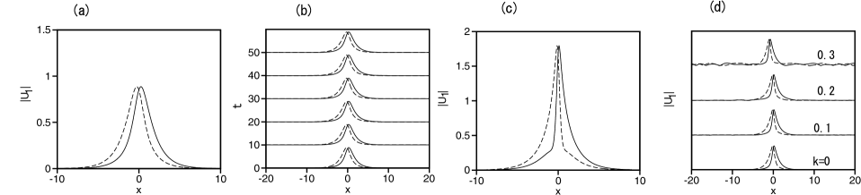
Figure 4: (a) Numerically obtained stationary solutions $|u_{1}(x)|$ and $|u_{2}(x)|$ (solid and dashed lines) of Eqs. (19 and (20) with $\Gamma=0.5$ and $\delta=1$ (the $\mathcal{PT}$-symmetric version of the system in which the intrinsic diffraction is omitted) at $k=-0.5$. (b) The perturbed evolution of component $\left|U_{1}\left(x,t\right)\right|$ of the same soliton.(c) The numerically obtained stationary soliton with $k=0.6$. (d) Results of the perturbed evolution of the solitons with $k=0$, $0.1$, $0.2$, and $0$ (all for $\Gamma=0.5$) at $z=900$, which reveal the location of the stability boundary at $k\approx 0.2$.

V Two-dimensional solitons

Numerical solution of the full 2D system of Eqs. (3) and (4) produces stable solitons too, which are characterized by the respective norm,

$$N=\int\int dxdt\left[\left|U_{1}(x,t)\right|^{2}+\left|U_{2}\left(x,t\right)\right|^{2}\right].$$ (31)

Examples of the 2D solitons are displayed in Figs. 5 and 6, which, in particular, demonstrate the mirror symmetry of $\left|U_{1}\left(x,t\right)\right|$ and $\left|U_{2}\left(x,t\right)\right|$. Note that, similar to what was observed above for 1D solitons, the increase of the SOC strength, $\delta$, generates a complex multi-lobe shape of the 2D solitons.

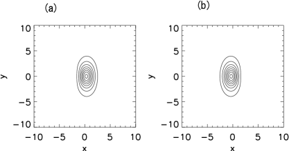
Figure 5: Contour plots of fields of fields $|u_{1}\left(x,t\right)|$ (a) and $|u_{2}(x,t)|$ (b) in a numerically found 2D soliton, at $\delta=1,\Gamma=0.2$, with norm $N=7.5$.

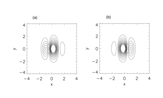
Figure 6: The same as in Fig. 5, but for $\delta=2,\Gamma=0.2$, and $N=7.1$.

As shown in Fig. 7, two different critical values of the norm can be identified for the 2D solitons. The upper one, $N_{\mathrm{c}}^{\mathrm{(upp)}}$, is the value at which, similar to what is found above for the 1D system, the $\mathcal{PT}$-symmetric solitons are destabilized by the spontaneous symmetry breaking. Specific to the 2D setting is a lower limit, $N_{\mathrm{c}}^{\mathrm{(low)}}$, below which the solitons cannot self-trap. At $N<$ $N_{\mathrm{c}}^{\mathrm{(low)}}$ simulations demonstrate spreading of the wave fields.

The existence of stable 2D solitons in the free space, under the action of the cubic-only attractive nonlinearity, is a nontrivial finding, as it was commonly believed that all solitons in such setting are destabilized by the (critical) collapse collapse ; Bilbao . Recently we , it was reported that the linear SOC terms may stabilize 2D solitons, as these terms break the specific scaling invariance of the 2D NLSEs, which accounts for the critical collapse in this case. The stability regions of the $\mathcal{PT}$-symmetric 2D solitons, demonstrated in Fig. 7, are a still stronger result, as the solitons are able to stay stable despite the simultaneous presence of two major destabilization factors: the possibility of the collapse, and the trend to spontaneous breakup of the balance between the gain and loss in the two cores of the coupler. It is pertinent to mention that other types of the SOC terms, which are relevant to two-component BEC, do not give rise to $N_{\mathrm{c}}^{\mathrm{(low)}}$, the respective stability region being $0<N<N_{\mathrm{c}}^{\mathrm{(upp)}}$ we . However, the $\mathcal{PT}$-symmetry cannot be introduced in a physically relevant form in that setting.

Naturally, Fig. 7(a) shows that the stability region found in the present system, $N_{\mathrm{c}}^{\mathrm{(low)}}<N<N_{\mathrm{c}}^{\mathrm{(upp)}}$, shrinks to nothing in the limit of $\delta\rightarrow 0$, when the 2D modes degenerate into the commonly known unstable Townes solitons collapse . On the other hand, a nontrivial finding is that the stability region attains its largest size at a finite value of the SOC strength, $\delta\sim 1$, as seen in Fig. 7. Similar to the 1D system [cf. Fig. 2(c)], the stability region keeps a (small) finite width at $\Gamma=1$, completely disappearing at $\Gamma>1$.

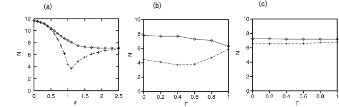
Figure 7: (a) The upper and lower critical values of norm (31) for the 2D solitons, as functions of the SOC strength $\delta$, for a fixed value of the gain-loss coefficient, $\Gamma=0.1$. (b) and (c) The critical values as functions of $\Gamma$ for $\delta=1$ and $\delta=2$, respectively. Stable 2D solitons exist between the continous and dashed critical lines.

VI Conclusion

The objective of this work is to introduce 1D and 2D optical systems which makes it possible to emulate the $\mathcal{PT}$ symmetry in combination with effects of the SOC (spin-orbit coupling), thus creating a novel physical setting. The systems are based on dual-core planar optical couplers with the Kerr nonlinearity in their cores. The $\mathcal{PT}$ symmetry is represented by equal amounts of the linear gain and loss in the two cores, while the SOC is induced by the skew form of the coupling between the cores. Families of stable 1D and 2D $\mathcal{PT}$-symmetric solitons have been identified by means of numerical and analytical methods. The size of the stability region of the 1D solitons nonmonotonously depends of the SOC strength, $\delta$, originally shrinking and then rapidly expanding with the increase of $\delta$. In the limit of the SOC terms dominating over the paraxial diffraction, the 1D system produces a new model for gap solitons, for which exact analytical solutions have been found. 2D solitons may be stable against the combined action of two major destabilization factors, viz., the critical collapse driven by the Kerr self-focusing, and the trend to spontaneous breakup of the balance between the gain and loss in the coupled cores.

The present analysis may be extended in other directions. In particular, it is interesting to consider the mobility of 1D and 2D solitons and collisions between them, which is a nontrivial problem in the presence of the SOC we . Dynamical regimes, such as Josephson-like oscillations of localized modes between the coupled cores, may be interesting too.

References

- (1) Bender C M and Boettcher S 1998 Phys. Rev. Lett. 80 5243; Bender C M, Brody D C and Jones H F 2002 ibid. 89 270401; Bender C M 2007 Rep. Prog. Phys. 70 947
- (2) Ruschhaupt A, Delgado F and Muga J G 2005 J. Phys. A: Math. Gen. 38 L171; El-Ganainy R, Makris K G, Christodoulides D N and Musslimani Z H 2007 Opt. Lett. 32 2632; Berry M V 2008 J. Phys. A: Math. Theor. 41 244007; Klaiman S, Günther U and Moiseyev N 2008 Phys. Rev. Lett. 101 080402; Longhi S 2009 ibid. 103 123601; Li K and Kevrekidis P G 2011 Phys. Rev. E 83 066608; Makris K G, El-Ganainy R, Christodoulides, D N and Musslimani Z H 2011 Int. J. Theor. Phys. 50, 1019; Ramezani H, Christodoulides D N, Kovanis V, Vitebskiy I and Kottos T 2012 Phys. Rev. Lett. 109 033902
- (3) Guo A, Salamo G J, Duchesne D, Morandotti R, Volatier-Ravat N, Aimez V, Siviloglou G A, and Christodoulides D N 2009 Phys. Rev. Lett. 103 093902; Rüter C E, Makris K G, El-Ganainy R, Christodoulides D N, Segev M, and Kip D 2010 Nature Phys. 6 192; Regensburger A, Bersch C, Miri M-A, Onishchukov G, Christodoulides D N and Peschel U 2012 Nature 488 167
- (4) Wiersma D S 2013 Nature Phot. 7 188; Segev M, Silberberg Y, and Christodoulides D N 2013 ibid. 7 197 (2013); Mafi A 2015 Adv. Opt. Phot. 7 459
- (5) Rechtsman M C, Zeuner J M, Plotnik Y, Lumer Y, Podolsky D, Dreisow F, Nolte S, Segev M, and Szameit A 2013 Nature 496 196
- (6) Plotnik Y, Rechtsman M C, Song D, Heinrich M, Zeuner J M, Nolte S, Lumer Y, Malkova N, Xu J J, Szameit A, Chen Z G and Segev M 2014 Nature Materials 13 57
- (7) Lin Y J, Jimenez-Garcia K and Spielman I B 2001 Nature 471 83; Zhai H 2012 Int. J. Mod. Phys. B 26 1230001; Spielman I B 2012 Ann. Rev. Cold At. Mol. 1 145; Galitski V and Spielman I B 2013 Nature 494 49; Zhou X, Li Y, Cai Z, and Wu C 2013 J. Phys. B: At. Mol. Opt. Phys. 46 134001; Goldman N, Juzeliūnas G, Öhberg P and Spielman I B 2014 Rep. Progr. Phys. 77, 126401
- (8) Kartashov Y V, Konotop V V and Malomed B A 2015 Opt. Lett. 40 4126
- (9) Kartashov Y V, Malomed B A, Konotop V V, Lobanov V E and Torner L 2015 Opt. Lett. 40 1045
- (10) Musslimani Z H, Makris K G, El-Ganainy R and Christodoulides D N 2008 Phys. Rev. Lett. 100 030402; Suchkov S V, Sukhorukov A A, Huang J, Dmitriev S V, Lee C and Kivshar Y S 2016 Laser Photonics Rev. 10 177; Konotop V V, Yang J and Zezyulin D A 2016 arXiv:1603.06826; Rev. Mod. Phys., in press
- (11) Wimmer M, Regensburger A, Miri M-A, Bersch C, Christodoulides D N and Peschel U 2015 Nature Communications 6 7782
- (12) Driben R and Malomed B A 2011 Opt. Lett. 36 4323; Alexeeva N V, Barashenkov I V, Sukhorukov A A and Kivshar Y S 2012 Phys. Rev. A 85 063837; Bludov Yu V, Konotop V V and Malomed B A 2013 Phys. Rev. A 87 013816
- (13) Burlak G and Malomed B A 2013 Phys. Rev. E 88 062904
- (14) Bergé L 1998 Phys. Rep. 303 259; Kuznetsov E A and Dias F 2011 ibid. 507 43; Fibich G, The Nonlinear Schrödinger Equation: Singular Solutions and Optical Collapse (Springer: Heidelberg, 2015).
- (15) Mardonov Sh, Sherman E Y, Muga J G, Wang H W, Ban Y and Chen X 2015 Phys. Rev. A 91, 043604
- (16) Sakaguchi H, Li B and Malomed B A 2014 Phys. Rev. E 89 032920
- (17) Wright E M, Stegeman G I and Wabnitz S 1989 Phys. Rev. A 40 4455; Paré C and Fłorjańczyk M 1990 ibid. 41 6287; Maimistov A I 1991 Kvantovaya Elektron. (Moscow) 18 758 (1991) [English translation: Sov. J. Quantum Electr. 21, 687 (1991)]
- (18) Chiang K S 1997 J. Opt. Soc. Am. B 14 143; Chiang K S 1997 IEEE J. Quantum Electron. 33 950
- (19) Chiofalo M L, Succi S and Tosi M P 2000 Phys. Rev. E 62 7438
- (20) Aceves A B and Wabnitz A 1989 Phys. Lett. A 141 37; Christodoulides D N and Joseph R I 1989 Phys. Rev. Lett. 62 1746
- (21) Malomed B A and Tasgal R S 1994 Phys. Rev. E 49 5787; Barashenkov I V, Pelinovsky D E and Zemlyanaya E V 1998 Phys. Rev. Lett. 80 5117; De Rossi A, Conti C and Trillo S 1998 ibid. 81 85