Black holes with constant topological Euler density

Abstract

A class of four dimensional spherically symmetric and static geometries with constant topological Euler density is studied. These geometries are shown to solve the coupled Einstein-Maxwell system when non-linear Born-Infeld-like electrodynamics is employed.

I Introduction

Since the discovery of Bekenstein Bekenstein1972 ; Bekenstein1973 ; Bekenstein1974 and Hawking Hawking1974 ; Hawking1975 connecting the entropy ($S$) and area ($\mathcal{A}$) of a black hole (BH), general relativity, quantum field theory and statistical physics became deeply linked. Not only in BHs does this connection work but also, as shown by Gibbons and Hawking Gibbons1977a , the cosmological horizon which is present in the de Sitter space fulfills $S=\frac{\mathcal{A}}{4}$. The geometric features of BH entropy seem to imply that it is related to the non-trivial topological structure of the corresponding spacetime. Moreover, Hawking and Gibbons Gibbons1977b argued that, due to the different topologies between extremal and non-extremal BHs, the area law fails for the former because their entropy vanish despite the non-zero area of the horizon. Furthermore, Teitelboim confirmed Teitelboim1995 , using the Hamiltonian formalism, that extremal BHs had zero entropy. These facts led Liberati and Pollifrone Liberati1997a to suggest the formula $S=\frac{\chi\mathcal{A}}{8}$, where $\chi$ is the Euler characteristic of the corresponding regular and Riemannian version of the considered spacetime (gravitational instanton). Although this formula has been checked for a wide class of gravitational instantons Liberati1997a ; Wang2000 ; Ma2003 , it is well know that it does not work in case of multiple horizon spacetimes Cai1998 .

The Euler characteristic of a gravitational instanton is related with a particular combination of curvature invariants of the form $\mathcal{G}=R^{\mu\nu\rho\sigma}R_{\mu\nu\rho\sigma}-4R^{\mu\nu}R_{\mu\nu}+R^{2}$ by means of the Gauss-Bonnet (GB) theorem. This GB term, $\mathcal{G}$, not only plays an important role in BH entropy but also in higher dimensional extensions of general relativity as well as in certain extensions in the four dimensional case. Specifically, the so-called $\mathcal{F}(\mathcal{G})$-gravity Nojiri2005 , where $\mathcal{F}$ is a non-linear function of the four dimensional GB invariant, produces late-time accelaration Nojiri2006 and is an interesting alternative to standard cosmology (see, for example, Ref. Felice2009 and references therein). Moreover, topological spherically symmetric vacuum solutions in $\mathcal{F}(R,\mathcal{G})$-gravity have been recently studied Myrzakulov2013 . Particularly, in Ref. Myrzakulov2013 , the authors looked for non-linear deformations of four dimensional $\mathcal{G}$- and $R$-gravity theories such that solutions with a constant $\mathcal{G}$ appear. In addition, the GB term is related to the trace anomalies in gravity (see Ref. Duff1994 for a review). Therefore, as pointed out in Ref. Gibbons1995 , the knowledge of the GB term may be also useful to know how this quantum anomaly affects the classical solutions.

In this work, a different intepretation of the static and spherically symmetric geometries supporting a constant $\mathcal{G}$ will be given in terms of non-vacuum solutions of standard Einsteinian gravity. Our interpretation is somewhat similar in spirit to that of Ref. Myrzakulov2013 but coupling certain model of non-linear electrodynamics (NLED) or null dust fluids (which generalize the Vaidya solutions Vaidya1951 ) to gravity, instead of deforming the gravitational action.

II Preliminaries: matter content

II.1 Non-linear electrodynamics

In geometrized units, Einstein equations ($\Lambda=0$) read

$$R_{\mu\nu}-\frac{1}{2}R\,g_{\mu\nu}=8\pi T_{\mu\nu},$$ (1)

where $T_{\mu\nu}$ is the energy-momentum tensor.

For the matter content we choose non-linear electromagnetic fields. To justify the study of these NLED theories, let us focus on two arguments. First of all, quantum corrections to Maxwell theory can be described by means of non-linear effective Lagrangians that define NLED as, for instance, the Euler-Heisenberg Lagrangian HE ; Sch . When higher order corrections are taken into account, we are led to a sequence of effective Lagrangians which are polynomials in the field invariants Bia . Among all the non-linear generalizations of Maxwell electrodynamics, Born-Infeld (BI) theory BI has been widely studied. Interestingly, the BI Lagrangian depends on the two field invariants in the same way as the one-loop effective Lagrangian for vacuum polarization due to a constant external electromagnetic field, which gives support to it. A second argument comes from the low-energy limit of string theory. Specifically, in case of dealing with open bosonic strings, the resulting tree-level effective Lagrangian is shown to coincide with the BI Lagrangian PLB1985 ; NPB1997 .

When coupled to gravity, NLED gives place to interesting phenomena. The corresponding solutions give place to generalizations of the Reissner-Nordström geometry, which have received considerable attention recently. In particular, BI solutions were presented in Garcia1984 ; Breton2003 . BH solutions for generalized BI theories were studied in Hendi2013 . An exact regular BH geometry in the presence of NLED was obtained in Ayon1998 and further discussed in Baldo2000 ; Bronni2001 . Finally, BHs with the Euler-Heisenberg effective Lagrangian as a source term were examined in Yajima2001 , and the same type of solutions with Lagrangian densities that are powers of Maxwell’s Lagrangian were analyzed in Hassaine2008 .

In this work we consider a simple choice for an energy-momentum tensor for NLED which is written as

$$T^{\mu\nu}=-\frac{1}{4\pi}\left[\mathcal{L}(F)g^{\mu\nu}+\mathcal{L}_{F}F^{\mu}_{\;\;\rho}F^{\rho\nu}\right]$$ (2)

where $\mathcal{L}$ is the corresponding Lagrangian, $F=-\frac{1}{4}F_{\mu\nu}F^{\mu\nu}$, and $\mathcal{L}_{F}=\frac{d\mathcal{L}}{dF}$ (along this work, dependence on the second field invariant, $\sqrt{-g}/2\epsilon_{\mu\nu\rho\sigma}F^{\rho\sigma}F^{\mu\nu}$, will not be considered).

For simplicity, let us take spherically symmetric and static solutions to Eqs. (1) given by

$$ds^{2}=-f(r)dt^{2}+f(r)^{-1}dr^{2}+r^{2}d\Omega^{2}.$$ (3)

In the electrovacuum case, we consider only a radial electric field as the source, namely,

$$F_{\mu\nu}=E(r)\left(\delta^{r}_{\mu}\delta^{t}_{\nu}-\delta^{r}_{\nu}\delta^{t}_{\mu}\right)$$ (4)

where $t$ and $r$ stand for the time and radial coordinates, respectively. Maxwell equations will now read

$$\nabla_{\mu}\left(F^{\mu\nu}\mathcal{L}_{F}\right)=0,$$ (5)

thus,

$$E(r)=-\frac{q}{r^{2}}(\mathcal{L}_{F})^{-1}.$$ (6)

As pointed out in Ref. Cherubini2002 , the non-Weyl part of the curvature determined by the matter content can be separated by showing that

$$4R^{\mu\nu}R_{\mu\nu}-R^{2}=(16\pi)^{2}\left(T^{\mu\nu}T_{\mu\nu}-\frac{T^{2}}{4}\right)$$ (7)

where $T=g^{\mu\nu}T_{\mu\nu}$ is the trace of the energy-momentum tensor. Therefore, in the considered spherically symmetric and static case, we arrive to the following expression for the electric field

$$E(r)=\frac{r^{2}}{4q}\sqrt{4R^{\mu\nu}R_{\mu\nu}-R^{2}}.$$ (8)

It is important to point out that Eq. (8) is also valid for $\Lambda\neq 0$, as can be easily shown by direct calculation.

Let us now check Eq. (8) in two particular cases. In the first case, we take a Reissner-Nordström BH whose relevant curvature invariants are given by $R^{\mu\nu}R_{\mu\nu}=\nobreak 4q^{4}/r^{8}$ and $R=0$. Therefore, $4R^{\mu\nu}R_{\mu\nu}-R^{2}=16q^{4}/r^{8}$ and $E(r)=q/r^{2}$, as expected.

In the second case, let us consider a regular BH metric Balart2014 given by $f(r)=1-\frac{2M}{r}e^{-\frac{q^{2}}{2Mr}}$. For this geometry, we get $R=e^{-\frac{q^{2}}{2Mr}}q^{4}/2Mr^{5}$ and $R^{\mu\nu}R_{\mu\nu}=e^{-\frac{q^{2}}{Mr}}q^{4}\left(q^{4}-8Mq^{2}r+32M^{2}r^{2}\right)/8M^{2}r^{10}$. Therefore, $4R^{\mu\nu}R_{\mu\nu}-R^{2}=e^{-\frac{q^{2}}{Mr}}q^{4}\left(q^{2}-8Mr\right)^{2}/4M^{2}r^{10}$ and $E(r)=\frac{q}{r^{2}}\left(1-\frac{q^{2}}{8Mr}\right)e^{-\frac{q^{2}}{2Mr}}$ which coincide with Eq. (19) of Ref. Balart2014 .

The underlying NLED theory can be obtained using the $P$ framework Salazar1987 , which is somehow dual to the $F$ framework. After introducing the tensor $P_{\mu\nu}=\mathcal{L}_{F}F_{\mu\nu}$ together with its invariant $P=-\frac{1}{4}P_{\mu\nu}P^{\mu\nu}$, one considers the Hamiltonian-like quantity

$$\mathcal{H}=2F\mathcal{L}_{F}-\mathcal{L}$$ (9)

as a function of $P$, which specifies the theory. Therefore, the Lagrangian can be written as a function of $P$ as

$$\mathcal{L}=2P\frac{d\mathcal{H}}{d{P}}-\mathcal{H}.$$ (10)

Finally, by reformulating the coupled Einstein-NLED equations in terms of $P$, $\mathcal{H}(P)$ is shown to be given by Bronnikov2001

$$\mathcal{H}(P)=-\frac{1}{r^{2}}\frac{d\mathcal{M}(r)}{dr}$$ (11)

where the mass function $\mathcal{M}(r)$ is such that $f(r)=1-\frac{2\mathcal{M}(r)}{r}$.

II.2 Null fluids

Let us consider the geometry in terms of (ingoing) Eddington-Finkelstein coordinates

$$ds^{2}=-f(r,v)dv^{2}+2drdv+r^{2}d\Omega^{2}$$ (12)

with $v=t+r$. The kind of metrics represented by Eq. (12) are a generalization of the Vaidya metric Vaidya1951 describing a spherically symmetric and nonrotating body which is either emitting ($u$-coordinate) or absorbing ($v$-coordinate) null dusts, i.e., “incoherent” electromagnetic radiation. Moreover, it can be seen Husain1996 ; Wang1999 that they solve the Einstein equations provided the associated energy-momentum tensor is that of a Type II perfect fluid book given by

$$T_{\mu\nu}=(\rho+p)(l_{\mu}n_{\nu}+l_{\nu}n_{\mu})+pg_{\mu\nu}$$ (13)

where $l_{\mu}=\delta^{t}_{\mu}$ and $n_{\mu}=\frac{1}{2}f(r)\delta^{t}_{\mu}-\delta^{r}_{\mu}$ are two null vectors. The density and pressure of the fluid are given by

$$\rho = \frac{\mathcal{M}_{r}}{4\pi r^{2}}$$

$$p = -\frac{\mathcal{M}_{rr}}{8\pi r}$$ (14)

where $\mathcal{M}_{r}\equiv d\mathcal{M}(r)/dr$.

At this point, it is noteworthy that for Type II fluids, the energy conditions read: (a) weak: $\rho\geq 0$ and $p+\rho\geq 0$, (b) strong: $p\geq 0$ and $p+\rho\geq 0$, and (c) dominant: $\rho\geq 0$ and $-\rho\leq p\leq\rho$.

III Solutions with constant topological Euler density

As mentioned in Refs. Nojiri2005 ; Nojiri2006 ; Myrzakulov2013 , several interesting cosmological models and topological static spherically symmetric solutions in $\mathcal{F}(R,\mathcal{G})$ gravity are obtained when the topological Euler density, i.e., $\mathcal{G}$, is constant. In addition, in $\mathcal{F}(\mathcal{G})$ gravity, during the transition from the matter to the accelerated era the topological Euler density is zero Felice2009 . For these reasons as well as for simplicity, we consider here solutions with constant topological Euler density.

The topological Euler density is defined as

$$\mathcal{G}=\frac{1}{32\pi^{2}}\left(R^{\mu\nu\rho\sigma}R_{\mu\nu\rho\sigma}-4R^{\mu\nu}R_{\mu\nu}+R^{2}\right).$$ (15)

For a spherically symmetric solution of the Einstein equations given by Eq. (3) we get

$$\mathcal{G}=\frac{4}{r^{2}}\left(f^{\prime}(r)^{2}+\left(f(r)-1\right)f^{\prime\prime}(r)\right)$$ (16)

with the factor $32\pi^{2}$ to have been included into $\mathcal{G}$ for convenience.

III.1 $\mathcal{G}=k\neq 0$ solutions

The solution of $\mathcal{G}=\nobreak k$ with $k$ to be an arbitrary constant is given by

$$f(r)=1\pm\sqrt{1-2A+Br+\frac{kr^{4}}{24}}$$ (17)

where $A$ and $B$ are arbitrary constants. Let us focus on the negative sign case which will give the BH solutions.

Employing Eq. (8), we get that Eq. (17) solves the Einstein-NLED system provided the electric field is given by

$$E(r)=\sqrt{6}\;\frac{4(1-2A)^{2}+48(1-2A)Br+27B^{2}r^{2}+(-1+2A)kr^{4}}{q\left(24-48A+24Br+kr^{4}\right)^{3/2}}.$$ (18)

At this point, a number of comments are in order. First, the electric field asymptotically will be

$$\lim_{r\rightarrow\infty}E(r)\rightarrow\sqrt{\frac{6}{k}}\frac{2A-1}{qr^{2}}$$ (19)

which corresponds to a Coulomb-like behavior with a charge $q^{2}=\sqrt{\frac{6}{k}}(2A-1)$. Second, if the constants are selected to be $A=1/2$ and $B=0$, then Eq. (17) corresponds to de Sitter or anti de Sitter space and its electric field vanishes, as shown by Eq. (18). Third, it is evident from Eq. (19) that the asymptotic electric field does not depend on $B$. Fourth, the metric element as given in Eq. (17) asymptotically reads

$$\lim_{r\rightarrow\infty}f(r)\rightarrow 1-\sqrt{\frac{6}{k}}\frac{B}{r}-\sqrt{\frac{6}{k}}\frac{2A-1}{r^{2}}-\sqrt{\frac{k}{6}}\frac{r^{2}}{2}$$ (20)

which corresponds to a Reissner-Nordström-de Sitter solution provided that

$$A = \frac{1}{2}+\frac{q^{2}\Lambda}{3}$$

$$B = \frac{4M\Lambda}{3}$$

$$k = \frac{8\Lambda^{2}}{3}.$$ (21)

Therefore, utilizing Eqs. (17) and (III.1), a BH solution of the coupled Einstein-NLED system for a certain electromagnetic Hamiltonian which will be derived in the Appendix, will be of the form

$$ds^{2}\!\!\! = \!\!\!-\left(1-\sqrt{\frac{4M\Lambda r}{3}+\frac{\Lambda^{2}}{9}r^{4}-\frac{2q^{2}\Lambda}{3}}\right)dt^{2}$$ (22)

$$\!\!\!+\frac{dr^{2}}{\left(1-\sqrt{\frac{4M\Lambda r}{3}+\frac{\Lambda^{2}}{9}r^{4}-\frac{2q^{2}\Lambda}{3}}\right)}+r^{2}d\Omega^{2}\leavevmode\nobreak\ .$$

Let us now study the massless ($M=0$) and massive ($M\neq 0$) cases, separately.

III.1.1 Massless case

In this case, the metric element as given in Eq. (22) now reads

$$ds^{2}\!\!\! = \!\!\!-\left(1-\sqrt{\frac{\Lambda^{2}}{9}r^{4}-\frac{2q^{2}\Lambda}{3}}\right)dt^{2}$$ (23)

$$\!\!\!+\frac{dr^{2}}{\left(1-\sqrt{\frac{\Lambda^{2}}{9}r^{4}-\frac{2q^{2}\Lambda}{3}}\right)}+r^{2}d\Omega^{2}\leavevmode\nobreak\ .$$

Depending on the values of the parameters, $q$ and $\Lambda$, of this metric, one gets:

• $q=0$ and $\Lambda\neq 0$
  This case corresponds to the de Sitter solution which has a cosmological horizon at $r_{c}=\nobreak(3/\Lambda)^{1/2}$.

• $q\neq 0$ and $\Lambda\neq 0$
  This case has an event horizon located at $r_{h}=\left[\frac{9}{\Lambda^{2}}+\frac{6q^{2}}{\Lambda}\right]^{1/4}$ with $\Lambda<-3/2q^{2}$. In addition, using Eqs. (18) and (III.1), the electric field reads

  $$E(r)=q\frac{r^{4}+6q^{2}/\Lambda}{\left(r^{4}-6q^{2}/\Lambda\right)^{3/2}}$$ (24)

  which asymptotically becomes, as expected,

  $$\lim_{r\rightarrow\infty}E(r)\rightarrow\frac{q}{r^{2}}\leavevmode\nobreak\ .$$ (25)

At this point, a number of comments are in order. First, the metric element, i.e., $f(r)$, of Eq. (23) can be written in the form

$$f(r) = 1-\frac{\Lambda}{3}r^{2}\sqrt{1-\frac{\alpha}{r^{4}}}$$ (26)

$$= 1-\frac{\Lambda}{3}r^{2}+\frac{q^{2}}{r^{2}}+\mathcal{O}\left(\alpha^{2}\right)$$

with $\alpha\equiv 6q^{2}/\Lambda$ to be a parameter that measures the deviation of the geometry described by the metric element given in Eq. (26) from de Sitter space. This deviation is depicted in Figure 1.

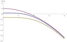
Figure 1: The red curve is the de Sitter space with $\Lambda=-1$, the blue curve is a spacetime with the metric function $f(r)$ to have $q=1$ and $\Lambda=-1$, and the olive green curve depicts a spacetime with metric function to have $q=2$ and $\Lambda=-1$.

Second, it is evident from Eq. (24) that there is an intrinsic singularity located at $r_{s}=\alpha^{1/4}$ with $\Lambda>0$. This singularity can also be detected if one computes the curvature invariants which, in this case, are given by

$$R^{\mu\nu\rho\sigma}R_{\mu\nu\rho\sigma} = \frac{8\Lambda\left(216q^{8}-144q^{6}r^{4}\Lambda+114q^{4}r^{8}\Lambda^{2}-18q^{2}r^{12}\Lambda^{3}+r^{16}\Lambda^{4}\right)}{3r^{4}\left(\Lambda r^{4}-6q^{2}\right)^{3}}$$

$$R^{\mu\nu}R_{\mu\nu} = 4\Lambda\left(\Lambda+\frac{2q^{4}\left(36q^{4}+60q^{2}r^{4}\Lambda-7r^{8}\Lambda^{2}\right)}{r^{4}\left(\Lambda r^{4}-6q^{2}\right)^{3}}\right)$$

$$g^{\mu\nu}R_{\mu\nu} = \frac{4\sqrt{\Lambda\left(-6q^{2}+r^{4}\Lambda\right)}\left(6q^{4}-9q^{2}r^{4}\Lambda+r^{8}\Lambda^{2}\right)}{r^{2}\left(\Lambda r^{4}-6q^{2}\right)^{2}}.$$ (27)

It should be stressed that, for $\Lambda>0$, the singularity $r_{s}$ will satisfy $r_{h}>r_{s}$ and, therefore, it will be an intrinsic singularity which will never become a naked one. Furthermore, this singularity can be avoided by choosing $\Lambda<0$. However, it is easily seen by inspecting the curvature invariants in Eq. (III.1.1) that another singularity is present. The singularity at $r=0$ becomes relevant in this case and, therefore, it is not possible a non-singular solution to be achieved although the electric field as given by Eq. (24) is regular everywhere. It is also noteworthy, that the singularity lying at the origin, i.e., at $r=0$, becomes a naked one when $\Lambda\geq-3/2q^{2}$.

III.1.2 Massive case

This is the general case so the metric element is the one given by Eq. (22)

$$ds^{2}\!\!\! = \!\!\!-\left(1-\sqrt{\frac{4M\Lambda r}{3}+\frac{\Lambda^{2}}{9}r^{4}-\frac{2q^{2}\Lambda}{3}}\right)dt^{2}$$ (28)

$$\!\!\!+\frac{dr^{2}}{\left(1-\sqrt{\frac{4M\Lambda r}{3}+\frac{\Lambda^{2}}{9}r^{4}-\frac{2q^{2}\Lambda}{3}}\right)}+r^{2}d\Omega^{2}\leavevmode\nobreak\ .$$

Several comments for this general case have been given at the beginning of this section. In the case that $q\neq 0$ and $\Lambda=0$, the geometry is that of Minskowski spacetime. Therefore, the case which will be studied now is the one with $q=0$ and $\Lambda\neq 0$. The corresponding curvature invariants are written as

$$R^{\mu\nu\rho\sigma}R_{\mu\nu\rho\sigma} = \frac{8}{3}\Lambda\left(\Lambda+\frac{4374M^{4}}{\left(12Mr+r^{4}\Lambda\right)^{3}}\right)$$

$$R^{\mu\nu}R_{\mu\nu} = \frac{4\Lambda\left(2754M^{4}+1620M^{3}r^{3}\Lambda+414M^{2}r^{6}\Lambda^{2}+36Mr^{9}\Lambda^{3}+r^{12}\Lambda^{4}\right)}{\left(12Mr+r^{4}\Lambda\right)^{3}}$$

$$g^{\mu\nu}R_{\mu\nu} = \frac{4\left(3M+r^{3}\Lambda\right)\sqrt{r\Lambda\left(12M+r^{3}\Lambda\right)}\left(15M+r^{3}\Lambda\right)}{\left(12Mr+r^{4}\Lambda\right)^{2}}\leavevmode\nobreak\ .$$ (29)

Here, a number of comments are in order. First, it is evident from Eq. (III.1.2) that provided $\Lambda>0$ the solution is regular everywhere except at $r=0$. Second, as no electric charge, i.e., $q=0$, is present in this case, the interpretation in terms of certain NLED is not of any interest. However, the corresponding source can be taken to be a Type II perfect fluid whose density and pressure are given, respectively, as

$$\rho = \frac{\Lambda\left(6M+r^{3}\Lambda\right)}{8\pi r\sqrt{r\Lambda\left(12M+r^{3}\Lambda\right)}}$$

$$p = -\frac{\Lambda^{2}\left(18M^{2}+18Mr^{3}\Lambda+r^{6}\Lambda^{2}\right)}{8\pi\left[r\Lambda\left(12M+r^{3}\Lambda\right)\right]^{3/2}}\leavevmode\nobreak\ .$$ (30)

Third, if $M\ll\Lambda$, then the corresponding spacetime will be a de Sitter one since the density and the pressure become, respectively,

$$\rho = \frac{\Lambda}{8\pi}\left(1+\mathcal{O}\left((M/\Lambda)^{2}\right)\right)$$

$$p = -\left[1-\frac{270M^{2}}{r^{6}\Lambda^{2}}+\mathcal{O}\left((M/\Lambda)^{4}\right)\right]\rho\leavevmode\nobreak\ .$$ (31)

Moreover, the pressure can also be written as

$$p=-\left[1-\frac{270M^{2}}{\Lambda^{2}r^{6}}+\mathcal{O}\left(\frac{1}{r^{9}}\right)\right]\rho$$ (32)

and, thus, the geometry becomes de Sitter also at spatial infinity.

Fourth, this solution satisfies both the weak and dominant energy conditions while the strong energy condition is violated due to the near-de Sitter behavior, as expected.

III.2 $\mathcal{G}=k=0$ solutions

The solution of $\mathcal{G}=\nobreak k=0$ is given by

$$f(r)=1\pm\sqrt{1-2A+Br}\leavevmode\nobreak\ .$$ (33)

We focus, as before, on the negative sign case which will give the BH solutions. In this case, the mass function reads

$$\mathcal{M}(r)=\frac{r}{2}\sqrt{1-2A+Br}$$ (34)

and the curvature invariants become

$$R^{\mu\nu\rho\sigma}R_{\mu\nu\rho\sigma}=\frac{\left(8+32A^{2}-32A(1+rB)+rB(16+9rB)\right)^{2}}{16r^{4}(1-2A+rB)^{3}}$$

$$R^{\mu\nu}R_{\mu\nu}=\frac{64(1-2A)^{4}-320r(-1+2A)^{3}B+608r^{2}(1-2A)^{2}B^{2}+504r^{3}(1-2A)B^{3}+153r^{4}B^{4}}{32r^{4}(1-2A+rB)^{3}}$$

$$R=\frac{8+32A^{2}-16A(2+3rB)+3rB(8+5rB)}{4r^{2}(1-2A+rB)^{3/2}}\leavevmode\nobreak\ .$$ (35)

Depending on the values of the constants, $A$ and $B$, the following cases are considered:

• $A=1/2$, $B=0$
  In this case, the geometry corresponds to Minkowski spacetime and the three energy conditions are trivially satisfied.

• $A<1/2$ and $B=0$
  In this case, there is a naked singularity located at $r=0$. In addition, the density and the pressure are given, respectively, as

  $$\rho = \frac{\sqrt{1-2A}}{8\pi r^{2}}$$

  $$p = 0\leavevmode\nobreak\ .$$ (36)

  Therefore, the weak, strong, and dominant energy conditions are satisfied provided $A<1/2$. Furthermore, this case corresponds to that of the gravitational field of a global monopole Barriola1989 ; Wang1999 with a deficit angle given by $\Delta=\sqrt{1-2A}$.

• $A=1/2$, $B>0$
  In this case, there is a horizon at $r=B^{-1}$ surrounding a singularity at $r=0$. In addition, the density and the pressure are given, respectively, as

  $$\rho = \frac{3\sqrt{Br}}{16\pi r^{2}}$$

  $$p = -\frac{3\sqrt{Br}}{64\pi r^{2}}\leavevmode\nobreak\ .$$ (37)

  Therefore, the weak and dominant, but not the strong, energy conditions are satisfied. It is noteworthy that this situation corresponds to a particular case of quintessence dark matter (see, for example, Ref. Ellis2012 ) whose equation of state is of the form $p=-\frac{1}{4}\rho$.

• $A\neq 0$, $B\neq 0$
  In this general case, the density and pressure are given, respectively, as

  $$\rho = \frac{2-4A+3Br}{16\pi r^{2}\sqrt{1-2A+Br}}$$

  $$p = -\frac{B(4-8A+3Br)}{64\pi r(1-2A+Br)^{3/2}}.$$ (38)

  It is easily seen that the most interesting case is when $0<2A<1$ and $B>0$. In this situation, there is a horizon at $r=2A/B$ surrounding the singularity at $r=0$. Both the weak and dominant energy conditions are satisfied when $r>0$. On the contrary, the strong energy condition is never fulfilled.

IV Discussion and conclusions

In this work we have studied a class of four dimensional spherically symmetric and static geometries with constant topological Euler density, i.e., $\mathcal{G}$, showing that they can be interpreted as Reissner-Nordström-de Sitter-like spacetimes when non-linear electrodynamics is utilized, or as generalized Vaidya solutions, depending on the value of $\mathcal{G}$.

In the first case in which the topological Euler density is a non-zero constant, i.e., $\mathcal{G}\neq 0$, we managed to show for the massless case, i.e., $M=0$, that the non-linear electric field can be regularized everywhere by taking $\Lambda<0$, although the geometry remains singular at $r=0$. Furthermore, it was shown that when $\Lambda\geq-3/2q^{2}$, the singularity lying at the origin, i.e., $r=0$, becomes naked. For the massive case, i.e., $M\neq 0$ when the charge is switched off, then provided that $\Lambda>0$, the obtained geometry is regular everywhere except the origin, i.e., $r=0$, where a singularity lies. In this situation, the source term is interpreted in terms of generalized Vaidya geometries. Contrary to the previous case, now both the density and pressure of the fluid become singular at $r=0$.

In the second case in which the topological Euler density is equal to zero, i.e., $\mathcal{G}=0$, the geometries obtained are that of Minkowski spacetime, of a global monopole, of a quintessence dark matter model, and of a BH with an horizon surrounding the singularity at $r=0$.

Finally, it should be stressed that, as stated in Garcia2012 , the only kinds of matter consistent with spherically symmetric and static gravitational fields in General Relativity are the cosmological constant vacuum, the anisotropic fluids, the perfect fluids, and the linear/non-linear Abelian/non-Abelian electromagnetic/Yang-Mills fields. Interestingly, as it was pointed out in Ref. Garcia2012 , this latter case also allows the interpretation of an anisotropic fluid in certain cases, one of which has been studied in the present work.

V Acknowledgments

P. B. acknowledges support from the Faculty of Science and Vicerrectoría de Investigaciones of Universidad de los Andes, Bogotá, Colombia.

VI Appendix

Using the dual formalism briefly described in section II, the underlying theory is shown to be given by

$$\mathcal{H}(P)=\left(-\frac{3}{2}\tilde{a}q+\frac{\tilde{b}P}{q}\right)\frac{1}{\sqrt{\tilde{a}q^{2}-2\tilde{b}P}}$$ (39)

with $\tilde{a}=\frac{\Lambda^{2}}{q}$ and $\tilde{b}=\frac{2}{3}q^{2}\Lambda$. Let us note that for small fields ($P\ll\Lambda$)

$$\mathcal{H}(P)=-\frac{\Lambda}{2}-P+12\sqrt{\Lambda}\,P^{2}+\mathcal{O}(P^{3})\leavevmode\nobreak\ .$$ (40)

At this point, it is worth of note that the BI Hamiltonian when expanded for small fields compared to the maximal field strength, $b$, reads

$$\mathcal{H}_{BI}=-F+\frac{F^{2}}{2b^{2}}+\mathcal{O}\left(F^{3}\right)\leavevmode\nobreak\ .$$ (41)

Therefore, the NLED model, described here, gives place to a BI-like model (up to $F^{2}$) when $b^{2}=\frac{1}{24\sqrt{\Lambda}}$.

References

- (1) J. D. Bekenstein, Lett. Nuovo cimento 4, 737 (1972).
- (2) J. D. Bekenstein, Phys. Rev. D 7, 2333 (1973).
- (3) J. D. Bekenstein, Phys. Rev. D 9, 3292 (1974).
- (4) S. W. Hawking, Nature 248, 30 (1974).
- (5) S. W. Hawking, Commun. Math. Phys. 43, 199 (1975).
- (6) G. W. Gibbons and S. W. Hawking, Phys. Rev. D 15, 2738 (1977).
- (7) G. W. Gibbons and S. W. Hawking, Phys. Rev. D 15, 2752 (1977).
- (8) C. Teitelboim, Phys. Rev. D 51, 4315 (1995).
- (9) S. Liberati and G. Pollifrone, Phys. Rev. D 56, 6458 (1997).
- (10) B. Wang, E. Abdalla and R-K Su, Phys. Rev. D 62, 047501 (2000).
- (11) Z. Z. Ma, Phys. Rev. D 67, 024027 (2003).
- (12) R-G. Cai, J-Y- Ji and K-S. Soh, Class. Quantum Grav. 15, 2783 (1998).
- (13) S. Nojiri and S. D. Odintsov, Phys. Lett. B 631, 1 (2005).
- (14) S. Nojiri, S. D. Odintsov and O. G. Gorbunova, J. Phys. A 39, 6627 (2006).
- (15) A. De Felice and S. Tsujikawa, Phys. Lett. B 675, 1 (2009).
- (16) R. Myrzakulov, L. Sebastiani and S. Zerbini, Gen. Rel. Gravit. 45, 675 (2013).
- (17) M. J. Duff, Class. Quantum Grav. 11, 1387 (1994).
- (18) G. W. Gibbons and R. E. Kallosh, Phys. Rev. D 51, 2839 (1995).
- (19) P. C. Vaidya, Por. Indian Acad. Sci. A 33, 264 (1951). Reprinted at Gen. Rel. Grav. 31, 119 (1999).
- (20) W. Heisenberg and H. Euler, Z. Phys. 98, 714 (1936).
- (21) J. Schwinger, Phys. Rev. 82, 664 (1951).
- (22) Z. Bialynicka-Birula, I. Bialynicki-Birula, Phys. Rev. D 2, 2341 (1970).
- (23) M. Born and L. Infeld, Proc. Roy. Soc. London A 144, 425 (1934); ibid. 143, 410 (1934) and 147, 522 (1934).
- (24) E. S. Fradkin and A. A. Tseytlin, Phys. Lett B. 163, 123 (1985).
- (25) A. A. Tseytlin, Nucl. Phys. B 501, 41 (1997).
- (26) A. García D., H. Salazar I. and J. F. Plebański, Nuovo Cimento Ser. B 84, 65 (1984).
- (27) N. Breton, Phys. Rev. D 67, 124004 (2003).
- (28) S. Hendi, Ann. Physics 333, 282 (2013).
- (29) E. Ayon-Beato and A. Garcia, Phys. Rev. Lett. 80, 5056 (1998).
- (30) F. Baldovin, M. Novello, S.E. Perez Bergliaffa and J. Salim, Classical Quantum Gravity 17, 3265 (2000).
- (31) K. A. Bronnikov, Phys. Rev. D 63, 044005 (2001).
- (32) H. Yajima and T. Tamaki, Phys. Rev. D 63, 064007 (2001).
- (33) M. Hassaine and C. Martinez, Classical Quantum Gravity 25, 195023 (2008).
- (34) S. Cherubini. D. Bini, S. Capozziello and R. Ruffini, Int. Journal Mod. Phys. D 11, 827 (2002).
- (35) L. Balart and E. C. Vagenas, Physical Review D 90, 124045 (2014).
- (36) H. Salazar I., A. García D. and J. Plebański, J. Math. Phys. 28, 2171 (1987).
- (37) K. A. Bronnikov, Phys. Rev. D 63, 044005 (2001).
- (38) V. Husain, Phys. Rev. D 53, R1759 (1996).
- (39) A. Wang and Y. Wu, Gen. Rel. Gravit. 31, 107 (1999).
- (40) S. W. Hawking and G. F. R. Ellis, The Large Scale Structure of space-time, Cambridge University Press, Cambridge (1979).
- (41) M. Barriola and A. Vilenkin, Phys. Rev. Lett. 63, 341 (1989).
- (42) G. F. R. Ellis, R. Maartens and M. A. H. MacCallum, Relativistic Cosmology, Cambridge University Press (2012).
- (43) A. Garcia, E. Hackmann. C. Lämmerzahl and A. Macías, Phys. Rev. D 86, 024037 (2012).