Criticality in Brownian ensembles
Abstract
A Brownian ensemble appears as a non-equilibrium state of transition from one universality class of random matrix ensembles to another one. The parameter governing the transition is in general size-dependent, resulting in a rapid approach of the statistics, in infinite size limit, to one of the two universality classes. Our detailed analysis however reveals appearance of a new scale-invariant spectral statistics, non-stationary along the spectrum, associated with multifractal eigenstates and different from the two end-points if the transition parameter becomes size-independent. The number of such critical points during transition is governed by a competition between the average perturbation strength and the local spectral density. The results obtained here have applications to wide-ranging complex systems e.g. those modeled by multi-parametric Gaussian ensembles or column constrained ensembles.
pacs:
PACS numbers: 05.40.-a, 05.30.Rt, 05.10.-a, 89.20.-aI Introduction
Recent studies of the localization to delocalization transitions e.g many body localization, Anderson localization and random graphs indicate a common mathematical structure underlying the statistical fluctuations of their linear operators krav ; psrp ; bgg . The structure belongs to that of a Rosenzweig-Porter (RP) ensemble rp , or, equivalently, to a specific type of Brownian ensemble (BE) i.e the one intermediate between Poisson and Gaussian ensembles psand . This indicates a crucial but so far hidden statistical connection of the BEs with systems undergoing localization-delocalization transition. It is therefore natural to search for the criticality in BEs which motivates the present study.
A Brownian ensemble in general refers to an intermediate state of perturbation of a stationary random matrix ensemble by another one of a different universality class dy ; me ; ap . The type of a BE, appearing during the cross-over, depends on the nature of the stationary ensembles and their different pairs may give rise to different BEs ap ; psijmp . Similar non-stationary states may also arise in other matrix spaces e.g. unitary matrix space e.g. due to a perturbation of a stationary circular ensemble by another one apps ; sp ; vp ; psnher . The BEs have been focus of many studies in past decades (for example see sp ; vp ; pslg and the references therein) and a great deal of analytical/ numerical information is already available about them. However very few of these studies alt ; psand ; krav probed the critical aspects of the BEs which refers to a behavior different from the two stationary limits in infinite matrix size limit mj . The search of criticality in BEs is important for several reasons. For example, the analytical study ps-all indicate that the statistical fluctuations of a wide range of complex systems are analogous to that of a Brownian ensemble, subjected to similar global-constraints, if their complexity parameters are equal irrespective of other system-details. (The complexity parameter is a function of the distribution parameters of the ensemble or alternatively a function of the average accuracy of the matrix elements, measured in units of the mean-level spacing). A recent study ss1 also reveals the connection of the BE to the random matrix ensembles with column/row constraints; the latter appear in diverse areas e.g bosonic Hamiltonians such as phonons, and spin-waves in Heisenberg and XY ferromagnets, antiferromagnets, and spin-glasses, euclidean random matrices, random reactance networks, financial systems and Internet related Google matrix etc. The knowledge of criticality in BEs can therefore be helpful in its search in other related ensembles.
The criteria for the critical statistics of energy levels and eigenfunctions was first introduced to an ensemble of disordered Hamiltonians undergoing localization to delocalization transition shk . It has long been believed that a fractional value of the spectral compressibility and multifractal behavior of the eigenfunctions are signatures of the criticality in the ensemble ckl ; azks . In fact these measures were used to claim the analogy of the Anderson ensemble (AE) at metal-insulator transition with that of the Power law random banded matrix (PRBM) ensemble prbm . The study psand ; pssymp indicates that the statistics of both of these ensembles can be mapped to that of the BEp→o (with subscript indicating the two end points i.e Poisson and Gaussian orthogonal ensemble); the BE is therefore expected to show similar critical features too. This is however at variance with another study krav which suggests the criticality in RP ensemble (and therefore in BEp→o) is different from AE and PRBME; this suggestion is based on a perturbative analysis of the eigenfunction fluctuations and two point spectral correlation (also see fkpt ; alt ; fgm ; ls ; ks for related studies). The need for a clear answer motivates us to pursue an analytical calculation of the spectral compressibility and multifractality for the BEs. Although our approach is applicable for a generic BE of both Gaussian or Wishart type (i.e intermediate between an arbitrary initial condition and the Gaussian/ Wishart type stationary ensembles, these measures so far seem to be relevant in context of the ensembles undergoing localization to delocalization transition. To strengthen and support the theoretical analysis, we probe the behavior by numerical route too but that is confined to the Gaussian BEs between Poisson to GOE only.
The paper is organized as follows. Section II briefly introduces the Brownian ensembles in Hermitian matrix spaces. The diffusive dynamics for their eigenvalues and the eigenfunction components was analyzed in detail in sp , pswf and pslg , respectively. This information is used in sections III and IV to derive the parametric dependence of the criticality measures i.e spectral compressibility, the multifractality spectrum and eigenfunction correlations at two different energies. Here we also discuss the conditions under which they become critical. Although the results of section III and section IV are applicable for arbitrary initial conditions, the main interest in these measures arises, so far, from the quest to characterize the localization to delocalization transition. This motivates us to focus on the corresponding BE i.e BEp→o in subsequent sections and numerically verify our theoretical results for them. Section V very briefly reviews the basic formulation for these BEs and presents the details of our numerical analysis. Section VI analyzes the reasons for the seemingly contradictory claims of the studies psand and krav . We believe it can be explained on the basis of a rate of change of the local density of states which affects the local statistical fluctuations. Section VII concludes with summary of our main results and open questions.
II Brownian ensembles: the definition
Introduced by Dyson to model the statistical behavior of systems with partially broken symmetries and/or approximate conservation laws dy ; me , a BE was originally based on the assumption of Brownian dynamics of matrix elements due to thermal noise. But currently a BE is also described as a single parameter governed diffusive state of the matrix elements of a randomly perturbed stationary ensemble me ; ap ; sp ; psijmp . Consider an ensemble of rectangular matrices with sp ; pslg and matrices and distributed with probability densities and . As clear, for , for . The ensemble of rectangular matrices can lead to three important classes of Hermitian matrix ensembles (i) Gaussian ensembles of matrices with , (ii) Wishart ensembles with matrices (also referred as Laguerre ensembles), and, (iii) Jacobi ensembles of matrices which approach a form . Our theoretical analysis in this paper is confined only to the first two ensembles.
A variation of strength of the random perturbation leads to diffusion of the matrix elements which, by a suitable choice of , can be confined to a finite space. For example, for the Gaussian density of the -ensemble, the Markovian character of the dynamics is preserved if considered in terms of a rescaled parameter given by the relation sp . For , the diffusion equation for the matrix elements of (with or ) can explicitly be derived sp ; pslg (with for as real-symmetric or complex Hermitian, respectively). As discussed in sp ; pswf ; pslg , this in turn leads to the -governed diffusion equation for the JPDF (joint probability distribution function) of their eigenvalues , and corresponding eigenfunctions. A direct integration of the JPDF diffusion equation over all eigenfunctions and eigenvalues leads to the diffusion equation for the order level-density correlation . The measure is also referred as the ensemble average level density, with its fluctuations described by , . As discussed in ap , the crossover in occur at a scale with as the local mean level spacing. The crossover in is however rapid and occurs at scale . For comparison of local spectral fluctuations around the level density, therefore, a rescaling of the eigenvalues by local mean level spacing (also referred as unfolding) is necessary. This however leads to a rescaling of both as well as the crossover parameter , with new parameter given as
| (1) |
with for Gaussian and Wishart ensembles respectively and is value of for initial ensemble .
As discussed in ps-all ; psand , also appears as the single parameter governing the spectral statistics of a multi-parametric Gaussian ensemble (which includes Gaussian BEs as a special case); in this case is the function of all ensemble parameters, thus containing information about the ensemble complexity. is therefore also referred as the spectral complexity parameter.
It must be emphasized here that, before unfolding, the correlations in a BE depends on two parameters, namely, local mean level density and perturbation parameter . Although the unfolding maps the local mean level density to a constant, it however introduces a spectral-scale dependence in the rescaled evolution parameter . The evolution of for is therefore different at different spectral scales which implies the non-stationarity of local fluctuations of the BE. This is different from the stationary ensembles in which correlations depends only on one parameter i.e local mean level density; the unfolding in this case results in a constant local level density and as a consequence, become independent of spectral scale.
Contrary to spectral correlations, the local eigenfunction correlations in a BE are governed by different rescaling of sensitive to the measure under consideration pswf ; pslg . This results in varying cross-over speeds for the eigenfunction fluctuations and is in fact an indicator of the multiple scale dependence of the local eigenfunction intensity.
III Signatures of criticality in spectral statistics
In general, the criticality in a joint probability distribution function (JPDF) of the eigenvalues can be defined as follows. A one-parameter scaling behavior of the distribution implies the existence of a universal distribution if the limit exists mj . Thus the size-dependence of plays a crucial role in locating the critical point of statistics. Let and , eq.(1) then gives . A variation of size in finite systems then leads to a smooth crossover of spectral statistics between an initial state () and the equilibrium (); the intermediate statistics belongs to an infinite family of ensembles, parameterized by . However, for system-conditions leading to , the spectral statistics becomes universal for all sizes, being -independent; the corresponding system conditions can then be referred as the critical conditions (or point). It should be stressed that the system conditions satisfying the critical criteria may not exist in all systems; the critical statistics therefore need not be a generic feature of all systems.
At critical value , (for ) and therefore all spectral fluctuation measures are different from the two end points of the transition i.e and . Any of them can therefore be used, in principle, as a criteria for the critical statistics. A direct theoretical or numerical study of the JPDF of eigenvalues or the correlations is however not the most suitable approach for the analysis. This has in past led to introduction of many alternative measures mj e.g. nearest neighbor spacing distribution, number variance, spectral rigidity etc. me . An important aspect of these measures is their spectral scale dependence. As mentioned in previous section, the spectral correlations in BEs retain their energy-dependence through even after unfolding and are non-stationary i.e vary along the spectrum gmrr . Any criteria for the criticality in the spectral statistics can then be defined only locally i.e within the energy range, say , in which is almost constant. From eq.(1), which implies that is large only for regions where .
The - governed diffusion of the eigenvalues subjects the local spectral fluctuation measures also to undergo a similar dynamics. To determine their behavior at the critical point, it is necessary to first obtain the evolution equations for the relevant measures. The spectral compressibility being a popular measure as well as related to other criteria for spectral criticality, here we consider its evolution.
III.0.1 Spectral compressibility and its evolution
As mentioned in section I, the spectral compressibility is an often used criteria for the criticality statistics in the ensembles of disordered Hamiltonians. A characteristic of the long-range correlations of levels, it is defined as, in a range around energy ,
| (2) |
where is the two point level density correlation at an energy . As is related to another -point measure, namely, the number variance , (the variance in the number of levels in an interval of mean number of levels), can also be expressed as the -rate of change of mj ; azks ; ckl ): for large with . (As the interest is often in large -behavior of at a fixed energy , its dependence on energy is usually suppressed). In ckl , was suggested to be related to the multifractality of eigenfunctions: with as the fractal dimension and as the system-dimension. However numerical studies indicated the result to be valid only in the weak-multifractality limit evers . Later on, another criteria was introduced in terms of the level-repulsion (an indicator of short range correlation), measured by nearest- neighbor spacing distribution. The study shk showed that the nearest-neighbor spacing distribution turns out to be a universal hybrid of the GOE at small- and Poisson at large-, with an exponentially decaying tail: for . Here is a constant and is believed to be related to : .
For the spectrum of uncorrelated levels (no level repulsion) i.e Poisson ensemble, which gives . But for a classical ensemble (e.g. Gaussian orthogonal or Unitary ensembles), the well-known sum rule gives ; this implies that a classical ensemble corresponds to the maximum level repulsion (i.e zero compressibility) in the related symmetry class me ; psijmp . Clearly if , it characterizes a spectrum different from classical ensembles as well as uncorrelated spectrum. This characterization however is suitable only for the stationary spectrum (where unfolded spectral correlations are independent of the location along the energy axis). In case of the non-stationarity, the statistics varies along the energy-axis (even after unfolding) and one can at best define a local compressibility within an energy range ( total spectrum width) in which the local stationarity is valid. This led to introduction of the following criteria for criticality: the spectral statistics is believed to be critical if
| (3) |
(Note the order of limits on and are non-interchangeable. This leads to technical issues in numerical search for criticality in : the total number of levels in the spectrum being finite, the maximum range of allowed is , with and it is not easy to realize a large limit).
To determine from eq.(2), a prior information of is needed. Unfortunately an exact form of is known for very few BE cases e.g Poisson to GUE, GOE to GUE, uniform to GUE ap . But the condition for a fractional value of can be obtained by general considerations. As discussed in ap ; sp , a variation of perturbation strength of the BE subjects to undergo diffusion, described as
| (4) |
with as the -point level-density correlation and given by eq.(1). Note the above equation is applicable only locally i.e within spectral scale in which is almost constant and is translationally invariant. The latter allows one to write but -dependence enters through . By differentiating eq.(2) with respect to , followed by a substitution of eq.(4) and subsequent repeated partial integrations, leads to following approximated closed form equation for (suppressing -dependence of for clarity of presentation)
| (5) |
An integration over of the above equation now gives
| (6) |
where and . Further simplification of eq.(6) is possible based on following points (i) can also be expressed in terms of : with as the order cluster function me ; ap . (ii) the range of integral over in the definition of varies from to and our interest is in the limit followed by , (iii) as varies from , the main contribution to the integral over in comes from the neighborhood of . Thus although the range of integration varies from to , one needs to concern only with small -values, (iv) the cluster function vanishes if or or becomes large in comparison to the local mean level spacing me . In large -limit, therefore, one can approximate which leads to . Using the latter, can be expressed in terms of : . The lack of energy level correlations at large i.e for arbitrary , also gives
| (7) |
In the ordered limit , eq.(6) can now be reduced to following form
| (8) |
with and . Further insight however can be gained by the following reasoning. As , the dominant contribution to the integral over comes from the region near . (This can also be seen as follows. In general, the eigenvalues at distances more than a system-specific spectral-range, say around , are uncorrelated. Here is a crucial spectral-range, hereafter, referred as the Thouless energy, as in the context of disordered systems in which case usually . This implies for where , one can write . Due to symmetry, the first two terms cancel out leaving only the last term.) Thus is sensitive to the short range behavior of i.e degree of level-repulsion in the spectrum.
It is worth noting here the advantage of eq.(8) over eq.(2): although calculation of by both eq.(2) and eq.(8) depends on a prior knowledge of but later requires only its small-range behavior which can easily be derived from eq.(4), for arbitrary initial conditions, by neglecting the integral term. As an example consider the BE intermediate to Poisson and Gaussian orthogonal ensemble (GOE); the small-r solution of eq.(4) for this case can be given as where is the modified Bessel function. Substitution of the latter in , leads to
| (9) |
where with in Poisson limit.
Further insight in the large- behavior of can be derived through a governed evolution equation in the spectral-region. The steps are as follows. Eq.(2) gives,. In large- limit, this leads to the approximation
| (10) |
Substitution of above relations in eq.(5) gives governed evolution of for large (with as constants):
| (11) |
As , the and term on the right side of the above equation can be neglected for large and its integration over gives with (assuming for large ). This reveals a bootstrapping tendency of i.e the dependence of at large on its behavior near small . Also note as both and are dependent on spectral scale , is in general non-stationary along the spectrum.
IV Signatures of criticality in eigenfunction statistics
The basis-variant nature of an ensemble, which is often the case at the critical point, implies a correlation between the eigenvalues and the eigenfunctions. The special features of the spectrum at the criticality are therefore expected to manifest in eigenfunctions too. For example, as indicated by many studies of the localization delocalization transitions, the eigenfunctions within spectral range supporting critical statistics have multifractal structure. This has motivated three main criteria for the criticality in the eigenfunction fluctuations, namely, inverse participation ratio, multifractality spectrum and eigenfunction correlations at different energy. Here we analyze these measures in context of the Brownian ensembles.
IV.0.1 Inverse participation ratio and its evolution
The criticality in the wavefunctions is believed to manifest through large fluctuations of their amplitudes at all length scales and is often characterized by an infinite set of critical exponents related to the scaling of the moments of the wave-function intensity with system size evers ; mj . The moment of the wave-function intensity , also known as inverse participation ratio is defined as (equivalently in a -dimensional basis with as the component of wavefunction ). As revealed by the critical point studies of many disordered systems, an ensemble averaged reveals an anomalous scaling with size : with implying an ensemble average with as the system dimension; note for a BE. Here is a non-decreasing convex function with .
The continuous set of exponents are related to the generalized fractal dimension of the wave-function structure: . At critical point, is a non-trivial function of , with and for the eigenfunctions extended in a -dimensional space and for completely localized ones, respectively. Further, is also related to anomalous dimension which distinguishes a multifractal state from an ergodic one and also determines the scale-dependence of the wave-function correlations: with evers .
For spectral regions with almost constant level density, the parametric-evolution of the average inverse participation ratio for a generic BE of Gaussian or Wishart type can be given as pslg ; pswf
| (12) |
with symbol implying a local spectral averaging of a variable . Here , and , and for the Brownian ensembles of Gaussian and Wishart type, respectively.
The above equation clearly indicates the dependence of on the spectral scale and system size . For finite but large , it can further be approximated as . With (for large ), implying , the above gives where is the average localization length in case of the localized eigenfunctions: ; this is in agreement with other studies ravin . Further note, for , approaches a correct steady state limit, namely, XOE or XUE with X L or G: for and for evers .
As discussed in pslg , the local intensity (given by in pslg ) depends on the perturbation strength of a BE and is different for Gaussian and Wishart ensembles. For later reference, here we mention the result for a Gaussian BE: . For a BE appearing during Poisson to GOE or GUE, and, with , this gives and for . A comparison of the above result with then gives, for ,
| (13) |
This in turn implies all the fractal dimensions for large but finite of the BE are same: .
IV.0.2 Diffusion of multifractality spectrum
A well-known criteria for the multifractality is the singularity spectrum : it is defined as the fractal dimension of set of those points at which (with as system dimension) and is related to by a Legendre transformation . The number of such points in a lattice scales as . Following from the definition, is a convex function and satisfies a symmetry evers . This in turn implies a symmetry in anomalous dimension too: .
For the delocalized wavefunctions is fixed: but its spread increases in cross-over from the delocalized wave limit to the localized one. In case of an ensemble, can be expressed in terms of the distribution of the local intensity of a typical eigenfunction krav
| (14) |
where with as the system-dimension and . For systems with weak multifractality, is believed to be approximately parabolic evers : with . This in turn implies . Note, for a classical ensemble as well as BE.
For a classical ensemble, the eigenfunction are delocalized in the basis-space and with as a chi-square distribution me : for XOE and for XUE (with X=G, L). The corresponding is then
| (15) |
To derive -dependence of for a BE, we first invert the relation (14) which gives . As discussed in pslg , a variation of the parameter gives rise to the diffusion of (using the notation ):
| (16) |
where
| (17) |
with , as the Thouless energy and for Gaussian and Wishart type Brownian ensembles respectively.
A substitution of as a function of in eq.(16) leads to the diffusion equation for :
| (18) |
with
| (19) |
where is the differential operator
| (20) |
where depend on the nature of BE: for Gaussian BEs, for Wishart BEs. The appearance of in eq.(18) clearly indicates an energy-sensitivity of the multifractality spectrum: it is non-stationary along the energy axis.
A desirable next step would be to solve the above equation but it is technically complicated. To gain further insight, we first simplify eq.(18) by a local spectral averaging which gets rid of the : integrating eq.(18) over the energy range , while assuming to be locally stationary over the region, leads to
| (21) |
where . Based on size-dependence of , the above equation can further be reduced to a simple form. Noting that in the spectrum-bulk, with ), we can approximate, for , or equivalently for ,
| (22) |
This indicates a linear dependence of for regions : where and depend on the initial conditions: and .
For regions where , the first term with square bracket of eq.(21) dominate the 2nd term. This in turn leads to following condition on the possible solution:
| (23) |
Thus now must satisfy both eq.(22) as well as eq.(23) simultaneously; one possible solution in this case seems to be with . A linear -dependence of was indicated also by a previous study krav in context of BEs appearing between Poisson to GOE.
As mentioned above, previous studies of multifractal states have suggested a parabolic solution for in weak multifractality regime (with ). Following from eq.(18), such a solution can exist in a small neighborhood of with given by the size dependence of : . This can be seen by a substitution of in eq.(18) directly (assuming local stationarity) which gives where , , and with correspond to initial conditions.
.
IV.0.3 Diffusion of wavefunction correlations
As intuitively expected, the anomalous scaling behavior of the multifractal states is also reflected by the overlap of their intensities. For example, during metal-insulator transition, two wavefunctions say and are known to display following correlation: for with as the anomalous dimension, , , as the average level density and as the system dimension evers . It is therefore natural to seek the role of the correlations in context of criticality in BEs evers .
The two-point intensity correlation between two eigenstates, say and with eigenvalues respectively, for a matrix , can be defined as
| (24) |
(with implying component of the eigenfunction ). As intuitively expected, its ensemble average is related to the 2-point spectral correlation . This in turn connects the eigenfunction statistics in the critical regime to that of eigenvalues. As discussed in pslg for BEs, the perturbation by a stationary ensemble leads to an evolution of from an arbitrary initial condition which depends on both (with ) and is non-stationary. But for the local correlations i.e those for which a variation with respect to can be ignored, the -governed evolution can be approximated as
where with , for Gaussian BE and Wishart BE, respectively, are the rescaled energy with defined in eq.(1) and is the 2nd inverse participation ratio at energy .
In the stationary limit , it is easy to check that (using the relation for the stationary ensembles with ergodic eigenfunctions). An exact solution of the above equation for finite, non-zero is complicated but, for small-, it can be obtained by expanding in Taylor’s series around . As discussed in pslg ) the small- behavior of depends on the small- behavior of . For bulk regions where is almost constant and , one has .
For criticality considerations, an asymptotic behavior of is relevant which can be given as with coefficients depend on initial conditions and energy-range . For in the bulk of spectrum, is almost constant. Neglecting the terms containing , due to being smaller as compared to other terms (note ), this leads to three possible solutions corresponding to :
| (26) |
where (i) , for , (ii) , for , (iii) , for . Higher are given by the recursion relation
| (27) |
where . where is the Kronecker delta function: or for and , respectively.
As discussed above, for small-. It is therefore appropriate to consider the measure as the criteria for criticality: for and is universal but is system-dependent for (as in this case leading to ). For criticality considerations, therefore, the large- behavior is relevant. For many systems undergoing the localization to delocalization transition of eigenstates, the behavior of for is described by the Chalker’s scaling chalk : but for of the order of spectral band width krav1 . But, as clear from the above, the large behavior of for a BE depends on the initial conditions as well as location of the spectral scale ; here behavior can occur for in the bulk spectral regimes (as here the ensemble averaged inverse participation ratio is almost energy-independent). For BE cases near the edge or intermediate spectral region , with determined by the energy-dependence of the inverse participation ratio .
For critical BE cases, is -independent and some of the higher may become larger than . The behavior in the range around is then dominated by term. As an example, we consider the BE case with Poisson initial condition and in the bulk of spectrum for cases with with and . As for Poisson limit krav1 , this implies , for . From the above, we then have , , for and for . For a size-dependent , say such that , therefore, the dominant contribution comes from the terms which leads to for . But for a size-independent , rapidly increase with for ; this in turn leads to with subjected to the condition and given by eq.(27).
V Critical BE during Poisson GOE transition: numerical analysis
The theoretical results in sections II-IV are applicable to the critical Brownian ensembles of both Gaussian and Wishart type. For the numerical analysis, however, we focus on a specific Gaussian BE, namely, the one which appears during Poisson to GOE crossover (due to its relevance in context of localization to delocalization transition of the eigenfunctions).
Consider the transition in Gaussian ensembles with an initial state described by the ensemble density . For a complete localization of its eigenfunctions in the basis in which is represented, the initial spectral statistics belongs to the Poisson universality class. The perturbation, of strength , by a matrix taken from a GOE (when represented in the unperturbed basis and of variance ), subjects eigenfunctions to increasingly delocalize as a function of . The ensemble of matrices , with then corresponds to the Brownian ensemble during Poisson GOE transition; it is described by the probability density fgm ; ls ; alt ; shapiro ; pich ; to .
| (28) |
with and arbitrary ; here for or and for or . As mentioned in section II, the evolution of matrix elements is described in terms of the parameter which in this case becomes .
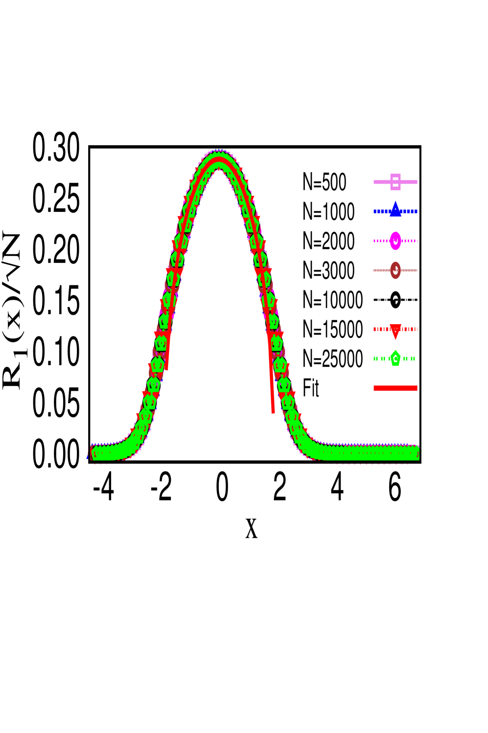
The standard route for the spectral statistical analysis is based on the fluctuations around the average level density. In the present case, the ensemble averaged level density , also known as order spectral correlation, changes from a Gaussian to a semi-circular form at the scale of : for respectively shapiro , with as an -independent constant. Although the exact form of the function is not known, our numerical analysis, displayed in figure 1, suggests a semicircle behavior in the spectral bulk i.e. with Gaussian tails and as a constant independent of . (Note the study shapiro gives for as a complex Hermitian matrix but the numerical evidence given in psand and in the present study confirms its validity also for the real-symmetric .) Clearly is non-stationary as well as non-ergodic bg ; as discussed below, this plays a crucial role in compressibility calculation.
As mentioned in section II, the spectral fluctuations around are governed by the parameter psand , given by eq.(1), which in this case becomes, with and mean level spacing ,
| (29) |
For finite , the -variation due to changing at a fixed energy results in a cross-over of the spectral statistics from Poisson () to GOE () universality class. In limit and for arbitrary , varies abruptly, approaching either or , ruling out possibility of any intermediate statistics. But if takes a value such that the limit exists, the statistics is then size-independent and belongs to a new universality class, different from the two end-points and is referred as the critical Brownian ensemble. As -dependence of also varies with , this implies the existence of two critical points (instead of one as previously discussed in alt ; shapiro ):
: as mentioned above, for this case behaves as a semi-circle in the bulk: . Although the behaviour near the edge is not known, the numerical analysis, displayed in figure 1 for , indicates a -scaling behaviour in all regions: is -independent. Eq.(29) then gives
| (30) |
with . Note, for , although is size-independent near the band-center , it is still quite large (), indicating the level-statistics to be close to the GOE. An intermediate statistics between Poisson and GOE can however be seen near for .
As mentioned in section IV.1, for Gaussian type BEs which gives, for this case, and in the bulk. This further implies and for the spectrum bulk which is in near agreement with our numerical result (which gives and , see figure 6(b)).
: as here , now becomes . From eq.(29), is again size-independent:
| (31) |
For , and the statistics lies between Poisson and GOE even for energy ranges near . As here , this gives , , which suggest a strong multifractal behavior (approaching localization) of the eigenfunctions; (note the latter rules out the validity of the relation in this case).
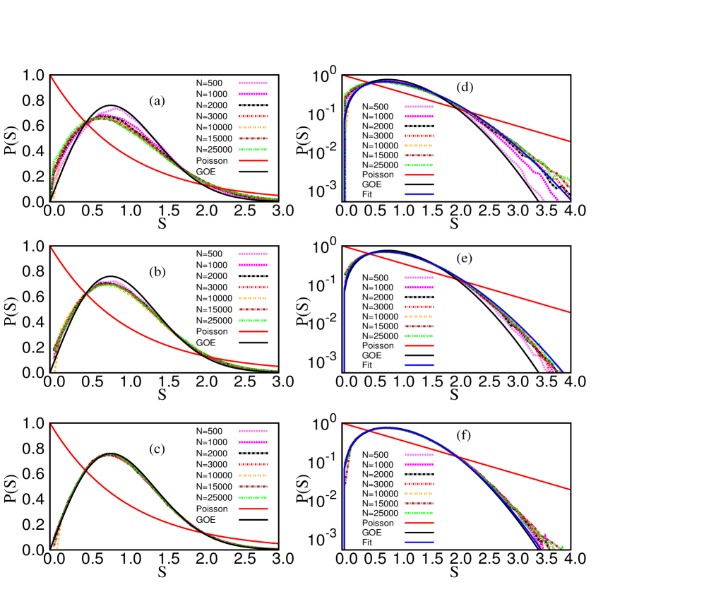
The theoretical formulations of the spectral compressibility and multifractal spectrum discussed in previous sections are based on a few approximations at various stages of the derivation. It is therefore desirable to verify the results by numerical route. The latter can also give an insight in critical point behavior of some other measures e.g nearest neighbor spacing distribution. The numerical evidence for the criticality for the case , with taken from a real-symmetric ensemble or complex-Hermitian ensemble, is discussed and verified in psand . The criticality of BE for this case but taken from a real-quaternion ensemble was numerically verified in pssymp (see figure 3 of pssymp ). In the present work, we pursue a numerical analysis of the case only. To understand the non-stationary aspects of critical statistics, we analyze three energy regime i.e . edge, bulk () or at intermediate energies (the region where is half of its maximum value). Although, due to rapid change in , the edge results are believed to be error-prone and thus a bit unreliable, but our results show a systematic trend which encourages us to include them in the figures here.
V.1 Critical spectral statistics
Our theoretical claim about criticality of BE at is based on a -dependence of the average level density . Our first step is therefore to numerically confirm its size-dependence. At this stage, an important question is regarding the ergodicity of the level density for the BE which implies , with as the spectral averaged level density; can then be used as a substitute for for various analytical purposes bg . The ergodicity is confirmed in a previous study ss1 (by a numerical comparison of the ensemble and the spectral averaging of the level density). It is therefore sufficient to analyze the size-dependence of . For this purpose, we consider the ensembles consisting of a large number of real-symmetric matrices, for many matrix sizes with ; the spectrum for each such ensemble is numerically generated using LAPACK subroutine based on an exact diagonalization approach. As shown in figure 1, is indeed semi-circle in the bulk but deviating from it near the edge. Further the -dependence is same for all energy ranges including edge as well as bulk.
As a next step, we analyze the spectral statistics which requires a careful unfolding of the spectrum. Due to unavailability of the analytical form of for all energy ranges, we apply the local unfolding procedure gmrr based on following steps: the smoothed level density for each spectrum is first determined by a histogram technique, and then integrated numerically to obtain the unfolded eigenvalues . The spectrum being non-stationary with energy-sensitive fluctuations (see figures 2,3 of ss1 ), it is necessary to analyze the statistics at different energy-ranges. For -based comparisons, ideally one should consider an ensemble averaged fluctuation measure at a given energy-point without any spectral averaging. But in the regions where varies very slowly, it is possible to choose an optimized range , sufficiently large for good statistics but keeps mixing of different statistics at minimum. We analyze 5 of the total eigenvalues taken from a range , centered at the energy-scale of interest i.e. edge, bulk and intermediate energies. (As for , in the bulk is almost constant, the statistics is locally stationary and one can take levels within larger energy ranges without mixing the statistics. A rapid variation of in the edge however permits one to consider the levels within very small spectral ranges only. For edge-bulk comparisons, it is preferable to choose the same number of levels for both spectral regimes). The number of matrices in the ensemble for each matrix size is chosen so as to give approximately eigenvalues and their eigenfunctions for the analysis.
To verify size-independence of the spectral statistics for , we consider and for the BE with for many system sizes. For comparison, it is useful to give their behavior in the two stationary limits:
(i) GOE: , with ,
(ii) Poisson: .
It is desirable to compare the BE-numerics with theoretical BE results too but the exact behavior for the BE with matrices of arbitrary size is not known. It is however easy to derive the for case to ; psbe : with as the modified Bessel function. As is dominated by the nearest neighbor pairs of eigenvalues, this result is a good approximation also for case, especially in small- and small--result to .
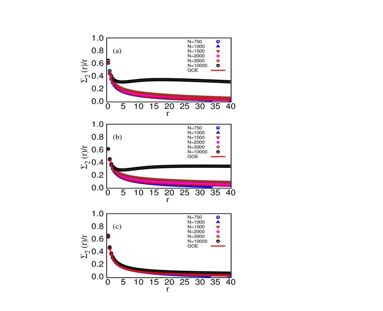
Figures 2, 3 and 4 display the behavior of and for the BE case for many system sizes ranging from to , in three energy regions. With for arbitrary (see fig.1), (given by eq.(30)) in this case is -independent but its value varies from edge to bulk: . As a consequence, the statistics is expected to be critical (i.e intermediate between Poisson and GOE) but different in the three spectral regimes. This is indeed in agreement with the behavior of the measures shown in fig.2, 3, 4. For , the statistics is nearer to GOE regime (fig.2(c,f), fig.3(c) and fig.4(c,f)) but its deviation from GOE increases for case with (fig.2(b,e), fig.3(b) and fig.4(b,e)). For near the edge, the statistics is expected to be closer to Poisson limit. Although this is confirmed by the tail behavior of shown in figure 2(d) and in 3(a) and 4(a,d), the small- behavior of is still far from Poisson limit (fig.2(a)). This clearly indicates the dependence of the speed of transition on the spectral ranges: although is small in this regime but for spectral ranges , the transition to GOE is almost complete.
The study shk suggests that an exponential decaying tail of the is an indicator for the critical spectral statistics. Fig.2(d,e,f) show a comparison of the tail behavior of with the curve where for levels taken from the edge, intermediate and bulk respectively. (Note, the fit is a close approximation of the theoretical formulation for mentioned above for a BE).
The compressibility can be numerically obtained from the large- limit of curves in figures 3,4; the numerical result is closer to our theoretical prediction (from eq. 9). Using (from eq.30), we get for the bulk () and intermediate regime () respectively. (The lack of information about exact in the edge handicaps us from a theoretical prediction for and therefore ). The small deviations from theory for smaller can be attributed to the spurious fluctuations due to finite size effects which affects the long-range statistics more severely. The true fluctuations are expected to be seen by going to limit. As can be seen from figure 4, for are closer to theory than . Note the bulk-value of is expected on the basis of relation too (valid for weak multifractal states in the bulk) chalk ; the latter gives with our numerically obtained . For partially localized states, has been suggested to be related to exponential decay of too shk : ; using for intermediate regime (given by P(s) fitting mentioned above), this gives which is again in agreement with our theory. (Note the range of validity of the relations and is different; the former is not applicable in near GOE regime and the latter is not valid in strong multifractal regime).
It must be emphasized that results are sensitive to the number of levels used for the analysis and the ensemble size even for ; figure 4 displays the change in behavior for different number of levels taken from a given regime for a given . As the compressibility calculation is based on a large limit of , its numerical evaluation for the ensembles of BE type (with rapidly changing level density) can not be reliable.
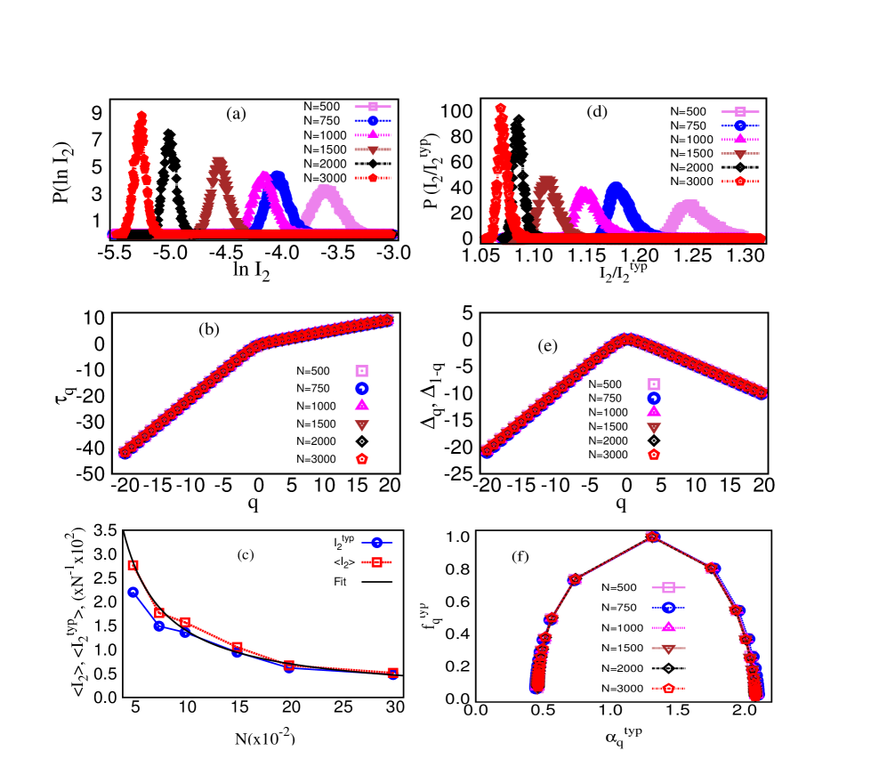
V.2 Multifractality analysis of wavefunctions
Our next step is to investigate the wavefunction statistics based on standard measures i.e inverse participation ratio (IPR), singularity spectrum and wavefunction correlations at two different energies.
In past, it has been conjectured that the distribution of normalized to its typical value has a scale-invariance at the localization-delocalization transition. This corresponds to a shape-invariance of with increasing system size , the latter causing only a shift of the distribution along axis evers . The above conjecture was questioned at first but confirmed later by numerical studies on Anderson transition for case (with as dimension) and critical power law random banded matrix (PRBM). To check its validity in case of the critical BEs, we numerically analyze the eigenstates for the case . To overcome finite size effects, one has to consider averages over different realizations of disorder as well as a narrow energy range. As these fluctuations in bulk are analyzed in detail in krav , here we confine ourselves to intermediate regime only. For this purpose, we consider the eigenstates in a narrow energy range 5 around intermediate energy for each matrix of the ensemble with , consisting of matrices, with for respectively. Figure 5(a) shows the distribution for the critical BE with ; the scale invariance of the distribution is clearly indicated from the figure. As indicated by previous studies evers , the -distribution is expected to show a power-law tail at the transition : for ; the behavior is confirmed in figure 5(d) for with ; (our numerics gives however a more detailed analysis is needed due to huge errors possible in tail of the distribution). Furthermore the change in peak-position of with changing system size confirms a power-law dependence of on system size , governed by a continuous set of exponents: where for .
As mentioned in section IV, the multifractal behavior of eigenfunction is described by a continuous set of scaling exponents evers . The latter can be computed by standard box-size scaling approach. This is based on first dividing the system of basis states into boxes ( is the dimension of the system and for our case, d=1) and computing the box-probability of in the box : ; here is over basis-states within the box. This gives the scaling exponent for the typical average of :
| (32) |
where is the average over many wavefunction at the criticality. For numerical calculation of , one usually considers the limit which can be achieved either by making or . We choose and carry out analysis for many values, each considered for an ensemble size ; (a large ensemble size is not required for their analysis). For case and , the slope of vs curve turns out to be which gives (see figure 5(b)) which agrees well with our theoretical prediction (see eq.(13)). This is also confirmed in figure 5(c) displaying -dependence of which is well-fitted by the expression . Rewriting in terms of , this implies and therefore reconfirms . Note, our result for is in contrast with the study krav which theoretically predicts for but numerical verifies the result only for the cases ).
Next we numerically analyze the singularity spectrum using box-approach in which and are defined as follows romer : and
| (33) |
with superscript on a variable implying its typical value. It is believed that the typical spectra is equal to the average spectra (i.e. and ) in the regime evers . Here correspond to the values of such that ; the corresponding value of are referred as , respectively. Our numerics of is confined within this regime. As displayed in figure 5(f) for six system sizes, behavior for the case is intermediate between the localized and delocalized limit. Also clear from the figure, is contained in the interval and satisfies the symmetry relation . The symmetry in the spectrum of can also be seen from the figure 5(e). Our analysis gives . Above results are consistent with expected multifractal characteristics of the critical eigenstates romer ; evers .
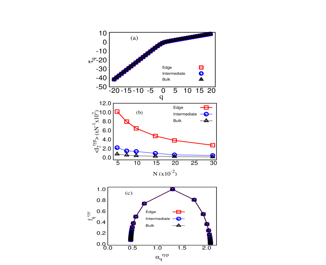
The non-stationarity of the spectral statistics and existence of non-zero correlations between eigenfunctions and eigenvalues suggest the multifractality measures to be sensitive to chosen energy-regime. This is also indicated by our theoretical analysis (see eqs.(20, 21) however a local spectral averaging almost hides the energy-dependence of . The main reason for this could be attributed to stronger sensitivity of the measures , to -dependence. Figure 6 compares the ensemble averaged , as well as singularity spectrum for three different energy ranges; although the energy dependence of is clear from fig.(b) but nearly same behavior of , indicates an almost insensitivity of these measures to the energy-scale. This is in contrast to spectral measures and where the non-stationary effects are more pronounced.
To reveal the non-stationarity effects on the eigenfunction fluctuation, it is therefore necessary to consider a measure in which energy-scales play an important role. As discussed in section IV.3, the 2-point wavefunction correlation is one such measure. Here we numerically analyze , given by eq.(24), for energy levels chosen in bulk () as well as in the intermediate-edge spectral regime. As discussed in section IV.3, the behavior of is expected to change near , with its curvature changing sign. Using the definition , with and , one has . As displayed in figure 7, the curvature of -curve indeed changes sign near , with increasing for and then undergoes a power law decay for . The decay however is faster than in both the regimes. As in this case is size-independent, this is in agreement with theoretical prediction (see end of section IV.3). The figure also displays different decay rates in the two regimes which is expected due to different spectral rate of variation of in the bulk and intermediate; as can be seen from fig.8(b), is almost constant in the bulk but increases rapidly around . This confirms the sensitivity of to the energy-regime of interest.
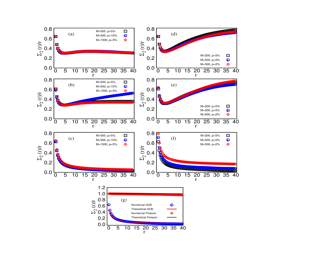
In the end, we compare our results for various critical measures with those in study krav . For an ensemble density described by eq.(28) with , the theoretical analysis of krav predicts (i) for , (ii) for ; here depends on : for and and respectively, (iii) for for all . Our theoretical analysis gives following results for the same ensemble: (i) for spectrum bulk for , (ii) a linear for and but possibility of a parabolic behavior near , (iii) for only in bulk and for (the latter corresponds to a size-dependent with ). being size-independent for , the large -decay of can be faster than . Our theoretical predictions are corroborated by the numerical analysis of case . ( Note the study krav presents -numerics for only). The deviation of our -result from krav may be due to their choice of a fixed size-dependence of the mean-level spacing () for all while we have used ; the latter result is derived in shapiro ) and is confirmed by our numerics too (see fig.1).
VI connection with other ensembles
A Gaussian Brownian ensemble is a special case of a multi-parametric Gaussian ensemble. As indicated by the studies ps-all ; psijmp ; psand , the eigenvalue distributions of a wide range of ensembles with single well potential e.g those with a multi-parametric Gaussian measure and independent matrix elements, appear as a non-equilibrium stages of a Brownian type diffusion process ps-all . Here the eigenvalues evolve with respect to a single parameter, say , which is a function of the distribution parameters of the ensemble. The parameter is related to the complexity of the system represented by the ensemble and can therefore be termed as the spectral ”complexity” parameter. The solution of the diffusion equation for a given value of the complexity parameter gives the distribution of the eigenvalues, and thereby their correlations, for the corresponding system. As the local spectral fluctuations are defined on the scale of local mean level spacing, their diffusion is governed by a competition between and local mean level spacing. Consequently the evolution parameter for the local spectral statistics is again given by eq.(1) but with a more generic definition of ; (note so far the complexity parameter formulation has been analyzed in detail only in context of Gaussian ensembles although the studies ps-all ; psnher indicate its validity for more generic cases). A single parameter formulation is also possible for the eigenfunction fluctuations but, contrary to spectral case, the parameter is not same for all of them pswf ; ps-all ; pslg .
The implications of the complexity parametric formulation are significant: as the system dependence enters through a single parameter in a fluctuation measure, its behavior for different systems with same value of the complexity parameter (although may be consisting of different combinations of the system parameters) will be analogous (valid for same global constraints; see ps-all for details). An important point worth emphasizing here is the following: although the unfolding (rescaling by local spectral density) of the eigenvalues removes their dependence on the local spectral scale, the latter is still contained in . The spectral dependence of varies from system to system. Thus two systems in general may have same spectral statistics at a given spectrum-point but the analogy need not extend for a spectral range of sufficient width. It could however happen in case the two systems have same local rate of change of along the spectrum which usually requires a similar behavior for the local spectral density. The analogy implied by the complexity parameter formulation is therefore strictly valid only in case of the ensemble averaging. It can however be extended to include spectral averaging within the range in which the local density is almost stationary.
The Anderson ensemble (AE) consisting of Anderson Hamiltonians, the power law random banded matrix (PRBM) ensemble and the Brownian ensemble appearing during Poisson GOE transition belong to same global symmetry class (time-reversal symmetry preserved). Based on the complexity parameter formulation, therefore, the critical point statistics of an AE or PRBME can be mapped to that of the Poisson GOE Brownian ensemble. The validity of the mapping was indeed confirmed by a number of numerical studies psand ; pssymp . As discussed in psand ; pswf ; pssymp , the critical BE analog of a critical AE is unique; similar to an AE, the level-statistics of the BE shows a scaling behavior too. The study krav however claims that the critical point behavior for an Anderson ensemble and a PRBM ensemble differ from that of a Rosenzweig-Porter ensemble (same as the Brownian ensemble between Poisson GOE cross-over). For example, the study shows that the correlation between two wavefunctions, at energies and decays as for , with for Rosenzweig-Porter ensemble and for Anderson Hamiltonian and PRBM ensemble. Here is the Thouless energy (same as used in context of BEs), with for AE and PRBME and for the BE. These results are however based on the assumption of local stationarity of the spectral density around which the fluctuations are measured. The seeming contradiction of the results between krav and psand originates in the range of validity of the assumption. As indicated by previous studies, the ensemble averaged bulk spectral density of an Anderson ensemble is almost similar in behavior as that of a PRBM ensemble but is different from that of the Poisson GOE Brownian ensemble. In the latter case, it varies more rapidly along the spectrum (see section V); the spectral range of local stationarity in case of the BE is therefore much smaller than the AE and PRBME and the measures (e.g. compressibility) which are based on large -limit considerations may not be appropriate for the comparison. Indeed the complexity parameter based formulation permits a comparison of the measures for each spectral point and is therefore more suitable for a comparative analysis of cases with different spectral-densities.
VII Conclusion
Based on a non-perturbative diffusion route, we find that the criticality of the fluctuation measures for the BEs is sensitive to both spectral scale as well as the perturbation strength. Our theoretical results are applicable for both Gaussian as well as Wishart BEs of the Hermitian matrices, with or without time-reversal symmetry and appearing during transition from an arbitrary initial condition to stationary ensembles. The results are confirmed by a numerical analysis of the BEs appearing during Poisson to GOE transition. The relevance of our BE-results is expected to be wide-ranging. For example, BEs are connected to the ensembles of column constrained matrices and latter has application in many areas discussed in ss1 . Further, using the complexity parameter based mapping of the fluctuation measures of a BE to a multi-parametric Gaussian ensemble ps-all , the results derived here are useful for the latter too.
An important outcome of our analysis is to reveal a new criteria for the criticality of the random matrix ensembles i.e the spectral complexity parameter. The latter has been shown to govern the evolution of all spectral fluctuation measures for a multi-parametric ensemble including BEs ps-all ; the search for criticality therefore need not depend on a specific measure e.g. compressibility. Using the complexity parameter, it is easier to find the number of critical points too: the spectral statistics has a critical point at a fixed energy if the size-dependence of the perturbation strength is same as that of the square of the mean level spacing. The appearance of two critical points in case of the BE between Poisson and GOE (i.e the Rosenzweig-Porter ensemble) can therefore be attributed to the variation of the level density from a Gaussian to semi-circle form. This also predicts the existence of two critical points in a Wishart Brownian ensemble which appears during Poisson to WOE transition;this follows because their level density changes from exponential decay to the form (with as a constant, see discussion below eq.(21) of pslg ). The existence of two critical points was recently reported in context of other complex systems too e.g. many body localization as well as random graphs krav1 .
The complexity parameter has an another advantage over previous measures for criticality which were often based on the assumption of the local ergodicity. As the search for the criticality originated in context of disordered systems, usually with large flat regions in the bulk level density, the local ergodicity considerations were easily satisfied. In general however this is not the case e.g. for systems with rapidly changing level densities. The measures based on the ensemble averaging only, or those based on averaging over very small spectral ranges are more appropriate choices to seek critical point in such cases.
The present work deals with the BEs taken from Hermitian matrix space. An understanding of critical BEs lying between the pairs of stationary ensemble subjected to other global constraints e.g. non-Hermiticity (.e.g. circular ensembles), chirality, column constraints still remains an open question.
References
- (1) V.E. Kravtsov, I.M. Khaymovich, E.Cuevas and M. Amini, New. J. Phys (IOP), (2016).
- (2) P. Shukla, New. J. Phys. (IOP), 18, 021004, (2016).
- (3) C.L.Bertrand and A.M. Garcia-Garcia, Phys. Rev. B 94, 144201, (2016).
- (4) N. Rosenzweig and C.E.Porter, Phys. Rev. 120, 1698 (1960).
- (5) P.Shukla, J.Phys.: Condens. Matter 17, 1653, (2005); Phys. Rev. E, 62, 2098, (2000).
- (6) F.Dyson, J. Math. Phys. 3, 1191 (1962).
- (7) M.L.Mehta,Random Matrices, Academic Press, (1991).
- (8) A. Pandey, Chaos, Solitons, Fractals, 5, 1275, (1995).
- (9) P. Shukla, Int. J. Mod. Phys. B (WSPC) 26, 12300008, (2012).
- (10) A. Pandey and P. Shukla, J. Phys. A, 24, 3907, (1991).
- (11) S. Kumar and A. Pandey, Ann. Phys. 326, 1877, (2011).
- (12) Vinayak and A. Pandey, Phys.Rev. E, 81, 036202 (2010).
- (13) P.Shukla, Phys. Rev. Lett., 87, 19, 194102, (2001).
- (14) P. Shukla, arXiv/submit/1673866.
- (15) A. Altland, M. Janssen and B. Shapiro, Phys. Rev. E, 56, 1471, (1997).
- (16) M. Janssen, Phys. Rep. 295, 1, (1998).
- (17) P. Shukla, J. Phys. A, 41, 304023, (2008); P.Shukla, Phys. Rev. E, (71), 026226, (2005); Phys. Rev. E, 62, 2098, (2000).
- (18) P.Shukla and S. Sadhukhan, J. Phys. A, , 48, 415003, (2015); J. Phys A, 48, 415002, (2015).
- (19) B.I.Shklovskii, B.Shapiro, B.R.Sears, P.Lambrianides and H.B.Shore, Phys. Rev. B, 47, 11487 (1993).
- (20) J.T.Chalker, V.E.Kravtsov and I.V.Lerner, Pis’ma Zh. Eksp. Teor. Fiz. 64, 355 (1996) [JETP Lett. 64, 386, (1996)].
- (21) B.L.Altshuler, I.Kh.Zharekeshev, S.A.Kotochigova and B.Shklovskii, Sov. Phys. JETP 67, 625, (1988).
- (22) A.D.Mirlin, Y.V.Fyodorov, F.-M. Dittes, J. Quezada and T.H.Seligman, Phys.Rev.E, 54, 3221, (1996).
- (23) R. Dutta and P.Shukla, Phys. Rev. E, 76, 51124, (2007).
- (24) J.B. French, V.K.B. Kota, A. Pandey and S. Tomsovic, Ann. Phys., (N.Y.) 181, 198 and 235 (1988).
- (25) K.M.Frahm, T.Guhr, A.Muller-Groeling, Ann. Phys. (N.Y.) 270, 292 (1998).
- (26) F. Leyvraz and T.H. Seligman, J. Phys. A: Math. Gen. 23, 1555, (1990).
- (27) H.Kunz and B.Shapiro, Phys. Rev. E, 58, 400, (1998).
- (28) P. Shukla, Phys. Rev. E, 75, 051113, (2007).
- (29) J.M.G. Gomez, R.A.Molinas, A. Relano and J. Retamosa, Phys. Rev. E, 66, 036209, (2002); O. Bohiga and M.J.Giannoni, Ann. Phys. 89, 422, (1975); I.O.Morales, E.Landa, P.Stransky and A.Frank, Phys. Rev. E, 84, 016203 (2011).
- (30) F. Evers and A.D. Mirlin, Rev. Mod. Phys, 80, 1355, (2008).
- (31) R. Bhatt and S. Johri, Int. J. Mod. Phys. Conf. Ser. 11, 79 (2012).
- (32) J. T. Chalker, Physica A 167, 253, (1990); J.T. Chalker and G.J. Daniell, Phys. Rev. Lett., 61, 593, (1988).
- (33) E. Cuevas and V.E. Kravtsov, Phys. Rev. B, 76, 235119, (2007).
- (34) M. Krenin and B. Shapiro, Phys. Rev. Lett., 74, 4122, (1995); B. Shapiro, Int. J. Mod. Phys. B, 10, 3539, (1996).
- (35) J-L. Pichard and B. Shapiro, J. Phys. I: France 4, 623, (1994).
- (36) S.Tomsovic, Ph.D Thesis, University of Rochester (1986); G.Lenz and F.Haake, Phys. Rev. Lett. 67, 1, (1991); V.K.B.Kota and S.Sumedha, Phys. Rev. E, 60, 3405, (1999).
- (37) O. Bohigas and M.J.Giannoni, Ann. Phys. 89, 393, (1975).
- (38) M.V. Berry and P. Shukla, J. Phys. A, Math.Theo. 42, 485102, (2009).
- (39) A. Rodriguez, L.J. Vasquez and R.A.Romer, arXiv:0807.4854v1 (2008).