The solar silicon abundance based on 3D non-LTE calculations

Abstract

We present three-dimensional (3D) non-local thermodynamic equilibrium (non-LTE) radiative transfer calculations for silicon in the solar photosphere, using an extensive model atom that includes recent, realistic neutral hydrogen collisional cross-sections. We find that photon losses in the Si i lines give rise to slightly negative non-LTE abundance corrections of the order $-0.01\,\mathrm{dex}$. We infer a 3D non-LTE based solar silicon abundance of $\lg{\epsilon_{\mathrm{Si\odot}}}=7.51$. With silicon commonly chosen to be the anchor between the photospheric and meteoritic abundances, we find that the meteoritic abundance scale remains unchanged compared with the Asplund et al. (2009) and Lodders et al. (2009) results.

1 Introduction

Silicon is one of the most abundant metals, and has many astrophysical applications. With a solar abundance and ionisation energy comparable to those of iron, it is a significant electron donor in the atmospheres of cool stars, and a key source of opacity in the interiors of solar-type stars. This has direct implications on, for example, the predicted solar neutrino flux (Serenelli et al., 2009; Serenelli, 2016). As an $\alpha$-capture element, patterns in abundance ratios such as $\mathrm{\left[Si/Fe\right]}$ against $\mathrm{\left[Fe/H\right]}$, in the Milky Way disk (e.g. Chen et al., 2002), bulge (e.g. Howes et al., 2016), and halo (e.g. Cohen et al., 2007; Shi et al., 2009; Yong et al., 2013), provide insight into stellar nucleosynthesis and the chemical evolution of the Galaxy. Finally, silicon is commonly used (e.g. Scott et al., 2015a; Scott et al., 2015b; Grevesse et al., 2015) to set the meteoritic abundances (Lodders et al., 2009) on the same absolute scale as the solar photospheric abundances (Asplund et al., 2009), because silicon is the reference element in meteorites where hydrogen is depleted. (Others (e.g. Lodders et al., 2009) prefer to use a selection of elements to determine the scale factor but in practice the outcome is basically the same as when only employing silicon for the purpose.)

It is therefore important to have accurate stellar silicon abundance determinations, and particularly for the Sun. Unfortunately, errors can enter spectroscopic abundance analyses from a number of different places. Often, errors in the transition probabilities of the spectral lines used to carry out the abundance analysis have a large effect. This is an issue for silicon (e.g. Shchukina et al., 2012), for which few laboratory measurements have been made within the past thirty years, while theoretical calculations typically have relatively large uncertainties (see for example the critical compilation of Kelleher & Podobedova, 2008). Assuming such errors are not systematic, which however is often the case, they can be circumvented by basing the abundance analysis on some weighted mean inferred from many spectral lines. Once given reliable transition probabilities for hopefully many spectral abundance diagnostics, the main systematic errors in the classic spectroscopic methodology arise from the use of one-dimensional (1D) hydrostatic model atmospheres and from the assumption that the material is in local thermodynamic equilibrium (LTE; e.g. Asplund, 2005).

The problems with 1D hydrostatic model atmospheres stem from their unrealistic treatment of convection; since they neglect fluid motions and time evolution, 1D model atmospheres must therefore rely on the Mixing-Length Theory (MLT; Böhm-Vitense, 1958; Henyey et al., 1965), which comes with a number of free parameters that need to be calibrated. Furthermore, spectral lines generated from 1D model atmospheres are too narrow compared to observed line profiles because they neglect the Doppler shifts associated with the convective velocity field and temperature inhomogeneities, so two more free parameters, microturbulence and macroturbulence, must also be invoked in order to fit observed spectra (e.g Gray, 2008, Chapter 17). In contrast, 3D hydrodynamical model solar and stellar atmospheres successfully reproduce the observations to exquisite detail, including the line shapes, shifts and asymmetries (e.g. Asplund et al., 2000; Nordlund et al., 2009; Pereira et al., 2013).

There have been several detailed investigations into the departures from LTE in Si i lines in the solar photosphere. Non-LTE calculations based on 1D model atmospheres by Wedemeyer (2001) found non-LTE abundance corrections ($\lg{\epsilon_{\mathrm{NLTE}}}-\lg{\epsilon_{\mathrm{LTE}}}$) that are typically very slightly negative, and of the order $-0.01\,\mathrm{dex}$, a result later consolidated by Shi et al. (2008) using a more extensive model atom. The non-LTE calculations by Sukhorukov & Shchukina (2012) using 1D hydrostatic model atmospheres, and by Shchukina et al. (2012) using a 3D hydrodynamic model atmosphere and treating each column of the model atmosphere independently (i.e. the so-called 1.5D approximation), suggest slightly more severe abundance corrections of the order $-0.05\,\mathrm{dex}$. Beyond the Sun, there is evidence of much larger non-LTE effects in Si i lines (e.g. Shi et al., 2009; Shi et al., 2011; Shi et al., 2012; Bergemann et al., 2013; Tan et al., 2016).

Recent 1D non-LTE calculations by Mashonkina et al. (2016) suggest that the severity of the non-LTE effects in the afore-mentioned studies may have been overestimated. Mashonkina et al. (2016) utilized for the first time the collisional cross-sections of Belyaev et al. (2014) for excitation and charge-transfer with neutral hydrogen, which were calculated using the Born-Oppenheimer formalism. Using the model atom of Shi et al. (2008), and 1D MARCS hydrostatic model atmospheres (Gustafsson et al., 2008), Mashonkina et al. (2016) commented briefly that the new collisional data reduce the non-LTE effects to vanishingly small levels in metal-poor turn-off stars. This is a significant result because, prior to these cross-sections becoming available, the semi-empirical recipe of Drawin (1968, 1969), as formulated by Steenbock & Holweger (1984) or Lambert (1993), was used, typically with a global scaling factor $S_{\mathrm{H}}=0.1$. This recipe does not provide a realistic description of the physics of the collisional interactions, being based on the classical Thomson (1912) electron ionisation cross-section; it is typically in error by several orders of magnitude (e.g. Barklem, 2016).

The canonical solar photospheric silicon abundance itself has seen a slight downwards revision, from $\lg{\epsilon_{\mathrm{Si\odot}}}=7.55$ (Anders & Grevesse, 1989; Grevesse & Sauval, 1998), to $\lg{\epsilon_{\mathrm{Si\odot}}}=7.51$ (Asplund, 2000; Asplund et al., 2005; Asplund et al., 2009; Scott et al., 2015a). The most recent of these was based on a 3D LTE analysis of nine Si i lines and one Si ii line in the solar disk-centre intensity spectrum and adopting 1D non-LTE abundance corrections to the solar flux spectrum from Shi et al. (2008). Correcting 3D LTE abundances with 1D non-LTE abundance corrections in this way is not consistent; furthermore these abundance corrections were obtained prior to the calculations of Belyaev et al. (2014) for the neutral hydrogen collisional cross-sections. A detailed investigation using a 3D hydrodynamic model solar atmospheres and 3D non-LTE radiative transfer, with the best available atomic data, is therefore highly desirable.

In this paper we study the 3D non-LTE Si i line formation in a 3D hydrodynamic model solar atmosphere. To obtain accurate results we construct a realistic model atom that includes recent neutral hydrogen collision data from Belyaev et al. (2014). We use the same Stagger model solar atmosphere as that used by Scott et al. (2015a). This enables us to directly apply our derived abundance corrections to their 3D LTE results, and thereby obtain a consistent 3D non-LTE solar photospheric silicon abundance.

2 Method

2.1 3D non-LTE radiative transfer code

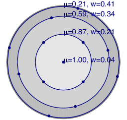
Figure 1: Projection of the unit sphere onto a 2D plane, illustrating the angle quadrature adopted for the statistical equilibrium calculations. The rings of constant $\mu$ and their weights $w$ are set by the $8\text{-point}$ Lobatto quadrature. The $\phi$ nodes on a given ring of constant $\mu$ are distributed evenly, and are given equal weight (i.e. equidistant trapezoidal quadrature). The $\phi$ nodes on different rings of constant $\mu$ are rotated relative to each other by $\frac{\uppi}{6}$ radians.

A customized version of Multi3D (Leenaarts & Carlsson, 2009) was used to solve for the statistical equilibrium (and to subsequently compute the emergent spectra), under the assumption that silicon is a trace element with no influence on the background pseudo-static model atmosphere (the so-called restricted non-LTE problem; Hummer & Rybicki, 1971). We refer the reader to the methodologies outlined in Amarsi et al. (2016a, b) for further details about the code.

We illustrate the angle quadrature that was used to calculate the mean radiation field during the statistical equilibrium calculations, in Fig. 1. A finer angle quadrature was adopted in this study than in the two afore-mentioned papers. For the integral over $\mu=\cos\theta$, an $8\text{-point}$ Lobatto quadrature on the interval [$-1,1$] was adopted, and for the integral over $\phi$ for the non-vertical rays, an equidistant $4\text{-point}$ trapezoidal integration on the interval [$0,2\uppi$] was adopted. This equates to $13\,\text{outgoing rays}$ on the unit hemisphere (Fig. 1), or $26\,\text{rays}$ over the unit sphere in total.

2.2 Model atmospheres

The model solar atmosphere used in this study was first presented by Asplund et al. (2009), and later tested against observational constraints by Pereira et al. (2013); it is the same model atmosphere used in the ongoing solar chemical composition series (Scott et al., 2015a; Scott et al., 2015b; Grevesse et al., 2015). It was computed using the Stagger code (Nordlund & Galsgaard, 1995; Stein & Nordlund, 1998), albeit with some customizations (e.g. Collet et al., 2011; Magic et al., 2013). We refer the reader to those studies for further details about the hydrodynamical simulations.

The original Cartesian mesh of $240\times 240\times 230$ (excluding the five ghost zones on the top and bottom of the simulation box) was reduced to $120\times 120\times 101$ for the 3D non-LTE calculations, to save computing time. This was done by selecting every second grid point in each of the horizontal dimensions, trimming optically deep layers (i.e. removing layers with vertical optical depth $500\,\mathrm{nm}$: $\lg{\tau_{500}}\gtrsim 3.0$). To test the impact of degrading the horizontal resolution, a 3D non-LTE test calculation was carried out using a single snapshot with $60\times 60\times 101$ resolution, and the equivalent widths were compared with those obtained from the same snapshot with $120\times 120\times 101$ resolution. The differences in the equivalent widths in the vertical intensity were minimal (of the order $0.00001\,\mathrm{dex}$ in the worst case). The differences in the equivalent widths in the inclined intensities were slightly larger (of the order $0.003\,\mathrm{dex}$ in the worst case), but still negligible for our purposes. The analysis presented in this work is based on abundance corrections derived from the equivalent widths in the vertical intensity. Hence we conclude that downgrading the horizontal resolution by a factor of four from $240^{2}$ to $120^{2}$ has no influence on the conclusions presented in this work.

Calculations were performed on six snapshots of the numerically-relaxed section of the full simulation, equidistant across $45.5\,\mathrm{minutes}$ of solar time. This number of snapshots was sufficient to obtain 3D non-LTE versus 3D LTE abundance corrections to a precision of better than $0.001\,\mathrm{dex}$, which could then be applied to the 3D LTE abundance derived by Scott et al. (2015a) that was based on a full sequence of snapshots. This time-sampling error of less than $0.001\,\mathrm{dex}$ in the abundance corrections was determined by comparing the abundance corrections derived from the individual snapshots with the final value obtained after integrating over the selected snapshots. The 3D non-LTE calculations were performed for three silicon abundances: $\lg{\epsilon_{\mathrm{Si\odot}}}=\{7.39\text{, }7.51\text{, }7.63\}$; the background chemical composition remained fixed using the abundances presented in Asplund et al. (2009). This resolution in silicon abundance was also sufficient to obtain interpolated 3D non-LTE versus 3D LTE abundance corrections to a precision of better than $0.001\,\mathrm{dex}$.

A horizontally- and temporally-averaged 3D model solar atmosphere (henceforth ⟨3D⟩) was constructed by averaging the gas temperature and logarithmic gas density from the 3D model atmosphere on surfaces of equal time and vertical optical depth at $500\,\mathrm{nm}$. All other quantities were then calculated consistently via the equation of state. In the ⟨3D⟩ model atmosphere the velocities were set to zero everywhere. As such, a microturbulent broadening parameter needed to be included in the line-formation calculations to account for the line broadening caused by convective motions; $\xi=1.0\,\mathrm{km\,s^{-1}}$ was adopted. We emphasize that these broadening effects are naturally taken into account when performing line-formation calculations in the 3D model atmosphere, without having to envoke any microturbulent broadening parameters (e.g. Asplund et al., 2000).

2.3 Model atom

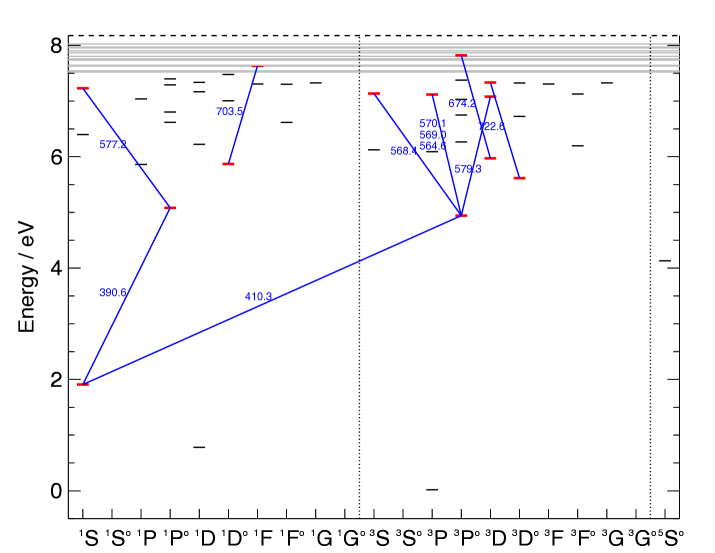
Figure 2: Grotrian diagram of the reduced model atom for which the statistical equilibrium was solved. Levels are shown in black; levels corresponding to the lines used in the subsequent analysis are shown in red, and these lines are also shown and labelled using their wavelengths in air in nanometres (c.f. Table 1). Twelve super levels are indicated in grey at the top of the diagram.

Table 1: Si i lines analysed in this work. The nine intermediate-excitation optical lines, and their parameters, correspond to those used by by Scott et al. (2015a) in their solar analysis. Two low-excitation violet Si i lines were also included in this study, but were not considered in the final solar abundance analysis. The oscillator strengths are those measured by Garz (1973), increased by $0.097\,\mathrm{dex}$ after renormalisation using the accurate lifetimes measured by O’Brian & Lawler (1991b, a).

$\lambda_{\text{Air}}/\mathrm{nm}$	Lower level	Upper level	$E_{\text{low}}$	$\log{g\,f}$
$390.553$	$3s^{2}\,3p^{2}\,\,{{}^{1}\mathrm{S}^{\text{}}_{0}}$	$3s^{2}\,3p\,4s\,\,{{}^{1}\mathrm{P}^{\text{o}}_{1}}$	$1.9087$	$-0.99$
$410.293$	$3s^{2}\,3p^{2}\,\,{{}^{1}\mathrm{S}^{\text{}}_{0}}$	$3s^{2}\,3p\,4s\,\,{{}^{3}\mathrm{P}^{\text{o}}_{1}}$	$1.9087$	$-3.04$
$564.561$	$3s^{2}\,3p\,4s\,\,{{}^{3}\mathrm{P}^{\text{o}}_{1}}$	$3s^{2}\,3p\,5p\,\,{{}^{3}\mathrm{P}^{\text{}}_{2}}$	$4.9296$	$-2.04$
$568.448$	$3s^{2}\,3p\,4s\,\,{{}^{3}\mathrm{P}^{\text{o}}_{2}}$	$3s^{2}\,3p\,5p\,\,{{}^{3}\mathrm{S}^{\text{}}_{1}}$	$4.9538$	$-1.55$
$569.043$	$3s^{2}\,3p\,4s\,\,{{}^{3}\mathrm{P}^{\text{o}}_{1}}$	$3s^{2}\,3p\,5p\,\,{{}^{3}\mathrm{P}^{\text{}}_{1}}$	$4.9296$	$-1.77$
$570.111$	$3s^{2}\,3p\,4s\,\,{{}^{3}\mathrm{P}^{\text{o}}_{1}}$	$3s^{2}\,3p\,5p\,\,{{}^{3}\mathrm{P}^{\text{}}_{0}}$	$4.9296$	$-1.95$
$577.215$	$3s^{2}\,3p\,4s\,\,{{}^{1}\mathrm{P}^{\text{o}}_{1}}$	$3s^{2}\,3p\,5p\,\,{{}^{1}\mathrm{S}^{\text{}}_{0}}$	$5.0823$	$-1.65$
$579.307$	$3s^{2}\,3p\,4s\,\,{{}^{3}\mathrm{P}^{\text{o}}_{1}}$	$3s^{2}\,3p\,5p\,\,{{}^{1}\mathrm{D}^{\text{}}_{2}}$	$4.9296$	$-1.96$
$674.164$	$3s^{2}\,3p\,4p\,\,{{}^{3}\mathrm{D}^{\text{}}_{3}}$	$3s^{2}\,3p\,8s\,\,{{}^{3}\mathrm{P}^{\text{o}}_{2}}$	$5.9840$	$-1.65$
$703.490$	$3s^{2}\,3p\,3d\,\,{{}^{1}\mathrm{D}^{\text{o}}_{2}}$	$3s^{2}\,3p\,5f\,\,{{}^{1}\mathrm{F}^{\text{}}_{3}}$	$5.8708$	$-0.78$
$722.621$	$3s\,3p^{3}\,\,{{}^{3}\mathrm{D}^{\text{o}}_{1}}$	$3s^{2}\,3p\,4f\,\,{{}^{3}\mathrm{D}^{\text{}}_{2}}$	$5.6135$	$-1.41$

2.3.1 Overview

The atomic physics of the non-LTE species is encapsulated in the model atom. The model atom needs to be complete and realistic in order to obtain reliable abundance corrections and an accurate solar photospheric silicon abundance. At the same time, the model atom needs to be small enough to permit 3D non-LTE calculations on the large model solar atmosphere used in this study. Similar to Bard & Carlsson (2008), our approach was to first construct a comprehensive model atom using the best available data (Sect. 2.3.2), and to subsequently reduce its complexity by collapsing fine structure levels and merging high-excitation levels into super levels (Sect. 2.3.3), while ensuring that the results from the reduced model atom remained consistent with those from the comprehensive model atom; these tests were done using the ⟨3D⟩ solar model atmosphere.

We illustrate the final, reduced model atom in Fig. 2. It consists of $56\,\text{levels}$ of Si i plus the ground state of Si ii and $634\,\text{radiative bound-bound transitions}$; all photoionisations between Si i levels and the ground state of Si ii are included. As with the comprehensive model atom used by Bard & Carlsson (2008), the model atom does not include any Si ii levels above the ground state. The first excited state of Si ii is $5.3\,\mathrm{eV}$ above the ground state, which means that their collisional coupling with Si i levels is minute. The excited states are also sparsely populated in the solar photosphere (e.g. Wedemeyer, 2001), implying that any non-LTE behaviour in the Si ii ion will have only a minute effect on the ground state of Si ii. Consequently, the excited states of Si ii are not expected to have any significant influence on the populations of Si i.

After the statistical equilibrium was solved for the reduced model atom, the populations were redistributed onto another model atom that had fine structure resolved, as described in Amarsi et al. (2016a). The emergent spectra were calculated for the (fine structure) lines listed in Table 1, which correspond to the nine intermediate-excitation Si i lines used by Scott et al. (2015a) in their solar analysis, as well as two low-excitation violet Si i lines that can be used the as the diagnostics for the structure of the solar chromosphere (Cincunegui & Mauas, 2001) and are also commonly used to determine the abundance of silicon in metal-poor stars (e.g. Cohen et al., 2007; Yong et al., 2013).

The oscillator strengths of the lines listed in Table 1 are based on those measured by Garz (1973) and renormalised using the accurate lifetimes measured by O’Brian & Lawler (1991b, a). A complication arises because they do not use LS coupling for the upper levels of three of the lines used here: the $674.2\,\mathrm{nm}$, $703.5\,\mathrm{nm}$, and $722.6\,\mathrm{nm}$ lines. For the first two of these levels, the corresponding LS coupling level can be uniquely determined via the LS coupling selection rules. For the third level, there is a choice of ${}^{3}D_{2}$ and ${}^{3}F_{2}$ levels; the former was adopted. The difference in the departure coefficients between these two levels in the line forming regions $-2\lesssim\lg{\tau_{500}}\lesssim 0$ is less than $0.01\%$ in the 3D model atmosphere snapshots; this implies that the choice has a negligible impact on the results.

2.3.2 Comprehensive model atom

Following Bard & Carlsson (2008), the main source of energies, oscillator strengths, and photoionisation cross-sections was the Opacity Project online database (TOPBASE; Cunto & Mendoza, 1992; Cunto et al., 1993). This data was computed under the assumption of strict LS coupling, and without any resolution of fine structure. The agreement with observed energies is typically at the 1% level, while the uncertainties in the oscillator strengths and photoionisation cross-sections are typically on the 10% level (Nahar & Pradhan, 1993).

The TOPBASE data set is relatively complete; a few missing Rydberg states with electron configurations of the form $3s^{2}\,3p\,nl$ were computed using the Rydberg formula, rCl E-E_∞&=-Ry(n-δl)2  , up to $0.2\,\mathrm{eV}$ below the ionisation limit, using a fit to the data from TOPBASE to roughly estimate the quantum defects $\delta_{l}$. Tests revealed that the presence of these extrapolated levels does not have a significant effect on the main findings of this paper; nevertheless they were retained in the model atom. Missing photoionisation cross-sections (including those for extrapolated levels) were estimated using a hydrogenic expression with Gaunt factors from Menzel & Pekeris (1935) as given in Gray (2008, Chapter 8).

The data was refined where possible using observed fine-structure energies from Martin & Zalubas (1983) and fine-structure oscillator strengths from various sources via the NIST online database (Kramida et al., 2015). As with the lines listed in Table 1, oscillator strengths from Garz (1973), were increased by $0.097\,\mathrm{dex}$ after renormalisation using the accurate lifetimes measured by O’Brian & Lawler (1991b, a).

The rate coefficients for excitation via electron collisions were calculated using the semi-empirical recipe of van Regemorter (1962). The Einstein coefficient for spontaneous emission enters into this recipe; for radiatively forbidden transitions the Einstein coefficient was calculated by assuming an effective oscillator strength $f_{\text{forb}}=0.001$. For ionisation via electron collisions the empirical formula given in Allen (1973, Chapter 3) was adopted.

The rate coefficients for excitation and charge transfer via neutral hydrogen collisions involving low- and intermediate-excitation Si i levels were taken from the calculations presented by Belyaev et al. (2014), based on the Born-Oppenheimer formalism. For charge transfer from high-excitation levels, and for excitation from low-excitation levels to high-excitation levels, the rate coefficients were obtained via fits in the $\lg{\left(\text{rate}\right)}\,\text{versus}\,\lg{\left(\Delta\,E\right)}$ plane. The excitation rate coefficients involving high-excitation levels were calculated via the free-electron model of Kaulakys (1985, 1986, 1991) in the scattering length approximation, using the routines presented by Barklem (2016).

Finally, collisional transitions within the same term were set to extremely large values to ensure that the corresponding fine-structure levels are populated according to their statistical weights and have identical departure coefficients (e.g. Kiselman, 1993).

2.3.3 Reduced model atom

Since the comprehensive model atom consists of over $50000$ frequency points, it was necessary to reduce the size of the model atom in order to make the 3D non-LTE calculations computationally tractable. To proceed, fine structure levels were collapsed into single levels. Following Martin & Wiese (1999), the average statistical weight and energy of a collapsed term $I$ are given by, rCl ¯g_I&=∑i∈I gi  ,
¯EI=∑i∈I giEi¯gI  , and the average wavelength and oscillator strength of a multiplet between two collapsed terms $I$, $J$ are given by, rCl ¯λ_I J&=h c¯EJ-¯EI  ,
¯f_I J= ∑i∈I,j∈J giλi jfi j¯gI¯λI J  .

Under the assumption that closely separated levels are collisionally coupled and thus have identical departure coefficients, levels above $7.5\,\mathrm{eV}$ separated by up to $0.04\,\mathrm{eV}$ were merged into super-levels, and affected radiative transitions were merged into super-transitions (e.g. Hubeny & Mihalas, 2014, Chapter 18). This merging was analogous to the collapsing of fine structure (Eq. 1 to Eq. 2.3.3), albeit with levels weighted by their Boltzmann factors $g_{i}\exp{\left(-E_{i}/k_{\mathrm{B}}\,T\right)}$ and using a characteristic temperature of $T=5000\,\mathrm{K}$, rather than simply their statistical weights $g_{i}$. Levels corresponding to lines to be used for the abundance analysis were not merged into super-levels (as illustrated in Fig. 2).

Lines with wavelengths greater than $10\,\mathrm{\mu m}$ were cut from the model atom. These lines do not significantly alter the statistical equilibrium, because they correspond to levels that are separated in energy by less than about $0.124\,\mathrm{eV}$; such levels are in close collisional coupling in the solar photosphere.

Tests on the ⟨3D⟩ model solar atmosphere revealed the error in the non-LTE equivalent widths in the vertical intensity incurred by collapsing the comprehensive model atom is less than $0.001\,\mathrm{dex}$. We suspect that the error incurred in the final 3D non-LTE results from collapsing the atom is insignificant compared to other uncertainties inherent in the model atom and hydrodynamical model atmosphere, and in the non-LTE radiative transfer calculations themselves.

3 Line formation in the solar photosphere

3.1 Non-LTE effect

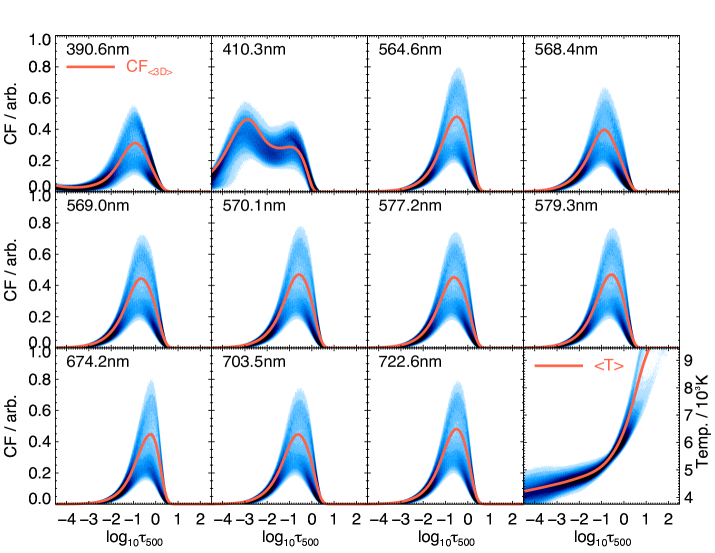
Figure 3: Non-LTE contribution functions to the line depression in the vertical intensity, integrated over frequency $\nu$: $\int{\alpha_{\nu}\,S^{\text{eff}}_{\nu}\,\mathrm{e}^{-\tau_{\nu}}\,\mathrm{d}\nu}$, where the vertical optical depth is $\tau_{\nu}$, the effective source function is $S^{\text{eff}}_{\nu}=\left(\alpha^{\mathrm{l}}_{\nu}/\alpha_{\nu}\right)\left(I^{\mathrm{c}}_{\nu}-S^{\mathrm{l}}_{\nu}\right)$, $\alpha_{\nu}$ and $S_{\nu}$ are the linear extinction coefficient and source function and $\mathrm{l}$ and $\mathrm{c}$ denote line and continuum quantities, respectively. This is shown for the eleven lines listed in Table 1, in arbitrary units (contours). Also shown are the corresponding contribution functions in the ⟨3D⟩ model atmosphere: $\mathrm{CF}_{\mathrm{\langle 3D\rangle}}$. For perspective, the bottom right panel shows the temperature stratification of the 3D and ⟨3D⟩ model solar atmospheres.

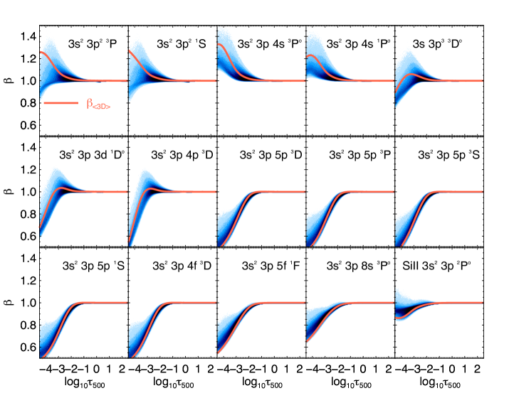
Figure 4: Departure coefficients $\beta=n^{\mathrm{NLTE}}/n^{\mathrm{LTE}}$ for the thirteen levels listed in Table 1, as well as the ground states of Si i and Si ii, in the 3D model atmosphere (filled contours). Also shown are the corresponding departure coefficients in the ⟨3D⟩ model atmosphere: $\beta_{\mathrm{\langle 3D\rangle}}$.

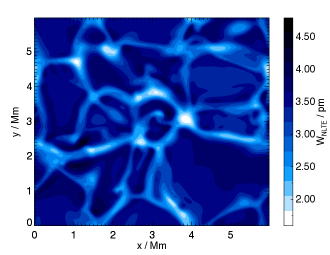
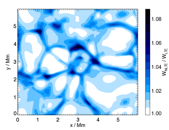
Figure 5: Non-LTE equivalent widths in the vertical intensity (left), and non-LTE to LTE equivalent width ratios in the vertical intensity (right), for the $564.6\,\mathrm{nm}$ line on the surface of a snapshot of the 3D model solar atmosphere for a fixed silicon abundance $\lg{\epsilon_{\mathrm{Si}}}=7.51$. The ratios are always greater than one or equal to one, indicating that the emergent equivalent widths are systematically stronger in non-LTE. The equivalent widths and equivalent width ratios for the other Si i lines listed in Table 1 take on a similar appearance.

To understand the non-LTE effect in individual lines, the line-forming regions must first be identified. We illustrate the Si i line-forming regions in the vertical intensity in Fig. 3. The intermediate-excitation Si i lines mostly form between $-2\lesssim\lg{\tau_{500}}\lesssim 0$. The two low-excitation Si i lines are saturated with significant optical depths even at the very top layers of the model atmosphere. This indicates that the solar model atmosphere may not be extended enough for these two lines, and thus that their absolute equivalent widths may not be reliable (although qualitative results for these lines remain useful); they were not considered in the abundance analysis of Scott et al. (2015a), and are consequently not considered in the abundance analysis presented here either.

We illustrate the departure coefficients, $\beta=n_{\text{NLTE}}/n_{\text{LTE}}$, in Fig. 4, for the ground states of the two ionisation stages, as well as for the levels we listed in Table 1. The plots reveal a generally smooth trend in the departure coefficients as a function of excitation energy. In the line-forming regions, the low-excitation Si i levels become overpopulated while the high-excitation Si i levels and the ground state of Si ii become underpopulated relative to their Saha-Boltzmann equilibrium populations.

The picture presented by the departure coefficients in Fig. 4 is characteristic of photon suction (Asplund, 2005): photon losses in the Si i lines drive a downward flow from the high-excitation levels to the low-excitation levels. Efficient coupling with the ground state of Si ii (mainly mediated by charge transfer with neutral hydrogen; Fig. 6) transfers population from the majority Si ii species into the minority Si i species, which further fuels the photon suction. The net effect is that the Si ii species becomes slightly underpopulated in the upper atmosphere while the Si i species as a whole becomes overpopulated relative to their Saha ionisation equilibrium populations; furthermore the lower levels of Si i become overpopulated while the higher levels of Si i become underpopulated relative to their Boltzmann excitation equilibrium populations.

We now consider the effects on the emergent equivalent widths of the lines we listed in Table 1. To a good approximation, the line opacities go as $\beta_{\text{lower}}$ and the line source functions go as the ratio $\beta_{\text{upper}}/\beta_{\text{lower}}$ (e.g. Rutten, 2003). As the lower levels of the intermediate-excitation Si i lines are overpopulated relative to their Saha-Boltzmann equilibrium populations, while their upper levels are underpopulated relative to their Saha-Boltzmann equilibrium populations, it follows that these lines are stronger in non-LTE than in LTE if given the same silicon abundance, by virtue of both an opacity effect and source function effect. In contrast, the lower and upper levels of the low-excitation Si i lines have similar departure coefficients in the line-forming regions: these lines are slightly stronger in non-LTE than in LTE if given the same silicon abundance, but only by virtue of an opacity effect.

We illustrate this line-strengthening effect in the vertical intensity across the surface of a single snapshot in Fig. 5. The departures from LTE are most severe in the intergranular downflows, a characteristic feature of photon losses (e.g. Amarsi et al., 2016b). In contrast, in the granular upflows the ratio of the non-LTE to LTE equivalent widths are close to unity. Since the granular upflows have the larger filling factor (by roughly a factor of two; e.g. Magic et al., 2013), the overall non-LTE effect on the equivalent widths is small.

3.2 3D versus ⟨3D⟩

It is interesting to briefly compare the average results obtained from the full 3D model at great computational cost, with those obtained from the average ⟨3D⟩ model at low computational cost. Before doing so we emphasize that all evidence suggests a full 3D analysis is required to obtain the highest accuracy, as gauged by spectral line strengths, shapes and continuum fluctuations across the solar disk (Pereira et al., 2009, 2013; Uitenbroek & Criscuoli, 2011). However, it may be that non-LTE calculations using ⟨3D⟩ model atmospheres present a reasonable compromise between computational cost and accuracy.

Qualitatively, the contribution functions in Fig. 3 behave similarly in the ⟨3D⟩ model as in the 3D model, for all of the lines considered in this study. This indicates that Si i line-forming regions are similar in the ⟨3D⟩ model atmosphere as in the 3D model atmosphere. The departure coefficients in Fig. 4 also show the same qualitative behaviour in the ⟨3D⟩ model atmosphere as in the 3D model atmosphere, at least in the layers $\lg{\tau_{500}}\gtrsim-3$. Quantitatively, we found that the ⟨3D⟩ LTE equivalent widths are typically about $0.01\,\mathrm{dex}$ stronger than the corresponding 3D LTE equivalent widths for the intermediate-excitation Si i lines. The ⟨3D⟩ non-LTE equivalent widths are also typically stronger than the corresponding 3D non-LTE equivalent widths, and by a similar amount. This suggests a reasonably cheap and accurate approach, as compared to the detailed 3D non-LTE radiative transfer approach, may be to apply ⟨3D⟩ non-LTE versus ⟨3D⟩ LTE abundance corrections to 3D LTE results. Before committing to this statement however, we shall have to perform similar investigations for other species, exhibiting different non-LTE effects, and for other types of stars.

3.3 Relative importance of radiative and collisional transitions

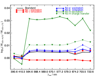
Figure 6: Non-LTE to LTE equivalent width ratios in the vertical intensity, in the ⟨3D⟩ model solar atmosphere for a fixed silicon abundance $\lg{\epsilon_{\mathrm{Si}}}=7.51$, when different radiative and collisional transitions are switched off. A larger ratio indicates a strengthening of the line in non-LTE (the LTE line widths are identical for each of the cases considered in this plot; hence this choice of normalization), and thus that the abundance corrections would be more negative.

We illustrate the relative importance of the different radiative and collisional processes in Fig. 6, which shows the non-LTE to LTE equivalent width ratios for the $11\,\mathrm{lines}$ in the ⟨3D⟩ model solar atmosphere for a fixed silicon abundance $\lg{\epsilon_{\mathrm{Si}}}=7.51$, when different radiative and collisional transitions are switched off.

Photon losses in the Si i lines are what drive the photon suction non-LTE effect we described in Sect. 3.1. Switching off all of the radiative bound-bound transitions in the statistical equilibrium calculations, impairs the population flow downwards from the higher levels of Si i into the lower levels of Si i. The level populations then become close to their Saha-Boltzmann equilibrium values in the line-forming regions, and, as we show in Fig. 6, the non-LTE effects in the Si i lines become negligible.

Collisional excitation has important thermalizing effects on the statistical equilibrium. Both electron collisions and neutral hydrogen collisions are efficient for transitions involving high-excitation Si i levels, ensuring their relative populations are given by Boltzmann statistics. For transitions involving low- and intermediate-excitation Si i levels, electron collisions are more important in the optically-thick atmosphere, whereas neutral hydrogen collisions are more important higher up in the Si i line-forming regions, where the hydrogen-to-free electron number ratio is larger. The neutral hydrogen collisions provide a key opposition to the effects of photon suction in the Si i lines of interest: as we show in Fig. 6, neglecting these collisions would significantly increase the predicted non-LTE effects, by about $0.03\,\mathrm{dex}$ in the solar case. Neglecting electron collisions while retaining neutral hydrogen collisions has only a perturbative effect on the line strengths, highlighting the dominance of the neutral hydrogen collisions.

Collisional ionisation has a significant effect on the statistical equilibrium in the line forming regions; as with collisional excitation, neutral hydrogen collisions have more effect on the final results than the electron collisions. Charge transfer reactions with neutral hydrogen efficiently link the intermediate-excitation Si i levels to the ground state of Si ii: this reduces the overpopulation of these Si i levels and reduces the underpopulation of the Si ii level, and brings the whole system closer to Saha-Boltzmann equilibrium. As we show in Fig. 6, the non-LTE effects are systematically larger when charge transfer reactions are neglected. In contrast, ionising electron collisions are more efficient for the high-excitation Si i levels. Their effect on the statistical equilibrium is complicated. They reduce the underpopulation of the higher Si i levels, bringing them closer to Saha-Boltzmann equilibrium, at the cost of directly increasing the underpopulation of the Si ii level, taking it further from Saha-Boltzmann equilibrium. This indirectly increases the overpopulation of the lower Si i levels by providing fuel for the photon suction effects. Consequently, while the non-LTE effects in the high-excitation Si i lines are larger when electron ionisation reactions are neglected, they are smaller in the low-excitation Si i lines.

Photoionisation does not have a substantial impact on the statistical equilibrium in the Si i line-forming regions, in contrast to the findings of Shi et al. (2008). This can perhaps be attributed to our inclusion of charge transfer by neutral hydrogen, which acts to balance to any potential overionisation or over-recombination effects.

4 Solar photospheric silicon abundance

Table 2: 3D non-LTE solar photospheric silicon abundances ($\lg{\epsilon_{\mathrm{3N}}}$) inferred from the nine high-excitation optical Si i lines. The abundance corrections $\Delta_{\mathrm{3N-3L}}$ are based on the theoretical equivalent widths that are consistent with the 3D LTE abundances ($\lg{\epsilon_{\mathrm{3L}}}$) that were inferred by Scott et al. (2015a) in the solar disk-centre intensity spectrum. Also shown is the single Si ii line at $637.137\,\mathrm{nm}$ that was analysed by Scott et al. (2015a). The Si ii line was included in the weighted mean used to obtain a final solar photospheric silicon abundance, under the assumption that it forms in LTE conditions (the derivation of abundance corrections for Si ii lines is beyond the scope of this work). The equivalent widths are those measured in the solar disk-centre intensity spectrum by Scott et al. (2015a), based on the average value obtained from the Kitt Peak atlas (Neckel & Labs, 1984; Brault & Neckel, 1987; Neckel, 1999)  and the Jungfraujoch atlas (Delbouille et al., 1973; Delbouille & Roland, 1995).

Species	$\lambda_{\text{Air}}/\mathrm{nm}$	Weight	$W/\mathrm{pm}$	$\lg{\epsilon_{\mathrm{3L}}}$	$\Delta_{\mathrm{3N-3L}}$	$\lg{\epsilon_{\mathrm{3N}}}$
Si i	$564.561$	$1.0$	$3.50$	$7.507$	$-0.008$	$7.499$
Si i	$568.448$	$2.0$	$6.37$	$7.464$	$-0.013$	$7.451$
Si i	$569.043$	$3.0$	$5.26$	$7.510$	$-0.011$	$7.499$
Si i	$570.111$	$3.0$	$3.95$	$7.491$	$-0.009$	$7.482$
Si i	$577.215$	$2.0$	$5.60$	$7.563$	$-0.010$	$7.553$
Si i	$579.307$	$1.0$	$4.58$	$7.601$	$-0.010$	$7.591$
Si i	$674.164$	$1.0$	$1.63$	$7.614$	$-0.004$	$7.610$
Si i	$703.490$	$1.0$	$7.40$	$7.552$	$-0.011$	$7.541$
Si i	$722.621$	$1.0$	$3.87$	$7.508$	$-0.009$	$7.499$
Si ii	$637.137$	$1.0$	$3.66$	$7.539$	$\left(-0.000\right)$	$\left(7.539\right)$

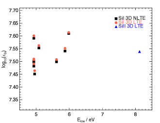
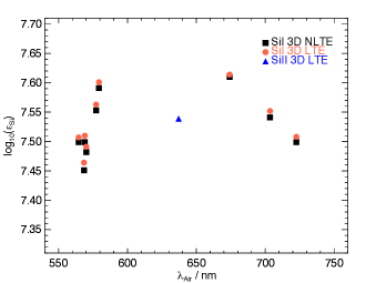
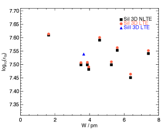
Figure 7: Solar silicon abundances inferred from the individual lines, as functions of: the excitation potential of the lower level of the lines; the wavelength of the lines; and the equivalent widths of the lines measured in the solar disk-centre intensity spectrum by Scott et al. (2015a).

We derived 3D non-LTE versus 3D LTE abundance corrections for each of the nine Si i lines analysed by Scott et al. (2015a) in the solar disk-centre intensity spectrum. For a given line, this was done by finding the theoretical equivalent width consistent with the 3D LTE abundance ($\lg{\epsilon_{\mathrm{3L}}}$) inferred by Scott et al. (2015a), and subsequently finding the 3D non-LTE abundance ($\lg{\epsilon_{\mathrm{3N}}}$) that corresponds to this equivalent width. The abundance correction is then $\Delta_{\mathrm{3N-3L}}=\lg{\epsilon_{\mathrm{3N}}}-\lg{\epsilon_{\mathrm{3L}}}$. This somewhat roundabout way is necessary since here we only average over six snapshots, while the 3D LTE study of Scott et al. (2015a) has a very fine sampling based on ninety snapshots across the same temporal range. We list the abundance corrections and inferred 3D non-LTE abundances for the individual lines in Table 2 and display them graphically as functions of the line parameters in Fig. 7. Our 3D non-LTE abundance corrections for the disk-centre intensity spectrum are very similar to the corresponding 1D non-LTE corrections for the solar flux spectrum of Shi et al. (2008) that were adopted by Scott et al. (2015a).

To obtain an estimate for the solar photospheric silicon abundance, a weighted mean was computed using our nine 3D non-LTE abundances from Si i lines, as well as the single Si ii line analysed by Scott et al. (2015a), (assuming that the 3D non-LTE abundance corrections for this latter line is zero as previous work using 1D radiative transfer has suggested; e.g. Shi et al., 2008; Bergemann et al., 2013). Using the weights of Scott et al. (2015a), we obtain $\lg{\epsilon_{\mathrm{Si\odot}}}=7.51\pm 0.03\,\mathrm{dex}$, adopting the same uncertainty as Scott et al. (2015a) that includes both statistical and systematic errors.

Our inferred solar photospheric silicon abundance is the same as advocated by Asplund (2000), Asplund et al. (2005), Asplund et al. (2009), and Scott et al. (2015a). This is reassuring; as discussed in Asplund et al. (2009), the canonical photospheric abundances are in excellent overall agreement with the corresponding meteoritic abundances (Lodders et al., 2009) when adopting this silicon abundance.

5 Conclusion

We have presented 3D non-LTE Si i line formation calculations using the 3D hydrodynamic Stagger model solar atmosphere of Asplund et al. (2009) and using a realistic model atom that includes recent quantum-mechanical neutral hydrogen collision data from Belyaev et al. (2014). Our main findings are:

• The non-LTE effect on the level populations is that of photon suction: photon losses in the Si i lines drive a population flow downwards, such that the lower levels are overpopulated and the higher levels are underpopulated, relative to their Saha-Boltzmann equilibrium populations.

• The non-LTE effects on the emergent equivalent widths are largest in the intergranular downflows, and nearly negligible in the granular upflows. The larger filling factor of the granular upflows make the overall 3D non-LTE versus 3D LTE abundance corrections are close to zero.

• We confirm the result of Mashonkina et al. (2016), that collisions with neutral hydrogen have a strong thermalizing effect on the statistical equilibrium. Excitation reactions provide a particularly important opposition to the photon suction effect.

• Applying our derived 3D non-LTE versus 3D LTE abundance corrections line-by-line to the 3D LTE solar photospheric silicon abundances derived by Scott et al. (2015a), we infer a 3D non-LTE solar photospheric silicon abundance of $7.51\,\mathrm{dex}$. This is the same as the current canonical value of Asplund et al. (2009) and Scott et al. (2015a), which had adopted 1D non-LTE abundance corrections.

We anticipate that future work on the solar photospheric chemical composition will increasingly utilize 3D non-LTE radiative transfer techniques such as those discussed in this paper; this is a necessary development for reducing the systematic modelling uncertainties to a level comparable to or better than the uncertainties associated with the observations and, in particular, the oscillator strengths of the diagnostic lines. Beyond the Sun, future theoretical work on neutral silicon may focus on the Si i $390.6\,\mathrm{nm}$ and $410.3\,\mathrm{nm}$ lines in the metal-poor regime ($\mathrm{\left[Fe/H\right]}\lesssim-2$), where strong UV overionisation effects are likely to drive positive non-LTE versus LTE abundance corrections of up to around $0.2\,\mathrm{dex}$.

References

- Allen (1973) Allen C. W., 1973, Astrophysical quantities. London: University of London, Athlone Press, —c1973, 3rd ed.
- Amarsi et al. (2016a) Amarsi A. M., Lind K., Asplund M., Barklem P. S., Collet R., 2016a, Non-LTE line formation of Fe in late-type stars - III. 3D non-LTE analysis of metal-poor stars, submitted
- Amarsi et al. (2016b) Amarsi A. M., Asplund M., Collet R., Leenaarts J., 2016b, MNRAS, 455, 3735
- Anders & Grevesse (1989) Anders E., Grevesse N., 1989, Geochimica Cosmochimica Acta, 53, 197
- Asplund (2000) Asplund M., 2000, A&A, 359, 755
- Asplund (2005) Asplund M., 2005, ARA&A, 43, 481
- Asplund et al. (2000) Asplund M., Nordlund Å., Trampedach R., Allende Prieto C., Stein R. F., 2000, A&A, 359, 729
- Asplund et al. (2005) Asplund M., Grevesse N., Sauval A. J., 2005, in Barnes III T. G., Bash F. N., eds, Astronomical Society of the Pacific Conference Series Vol. 336, Cosmic Abundances as Records of Stellar Evolution and Nucleosynthesis. p. 25
- Asplund et al. (2009) Asplund M., Grevesse N., Sauval A. J., Scott P., 2009, ARA&A, 47, 481
- Bard & Carlsson (2008) Bard S., Carlsson M., 2008, ApJ, 682, 1376
- Barklem (2016) Barklem P. S., 2016, A&A Rev., 24, 9
- Belyaev et al. (2014) Belyaev A. K., Yakovleva S. A., Barklem P. S., 2014, A&A, 572, A103
- Bergemann et al. (2013) Bergemann M., Kudritzki R.-P., Würl M., Plez B., Davies B., Gazak Z., 2013, ApJ, 764, 115
- Böhm-Vitense (1958) Böhm-Vitense E., 1958, Zeitschrift fuer Astrophysik, 46, 108
- Brault & Neckel (1987) Brault J., Neckel H., 1987, available from ftp. hs. uni-hamburg. de/pub/outgoing/FTS-Atlas/(Cité efinpage 69.)
- Chen et al. (2002) Chen Y. Q., Nissen P. E., Zhao G., Asplund M., 2002, A&A, 390, 225
- Cincunegui & Mauas (2001) Cincunegui C., Mauas P. J. D., 2001, ApJ, 552, 877
- Cohen et al. (2007) Cohen J. G., McWilliam A., Christlieb N., Shectman S., Thompson I., Melendez J., Wisotzki L., Reimers D., 2007, ApJ, 659, L161
- Collet et al. (2011) Collet R., Magic Z., Asplund M., 2011, Journal of Physics Conference Series, 328, 012003
- Cunto & Mendoza (1992) Cunto W., Mendoza C., 1992, Revista Mexicana de Astronomia y Astrofisica, 23
- Cunto et al. (1993) Cunto W., Mendoza C., Ochsenbein F., Zeippen C. J., 1993, A&A, 275, L5
- Delbouille & Roland (1995) Delbouille L., Roland C., 1995, in Sauval A. J., Blomme R., Grevesse N., eds, Astronomical Society of the Pacific Conference Series Vol. 81, Laboratory and Astronomical High Resolution Spectra. p. 32
- Delbouille et al. (1973) Delbouille L., Roland G., Neven L., 1973, Atlas photometrique du spectre solaire de [lambda] 3000 a [lambda] 10000. Liege: Universite de Liege, Institut d’Astrophysique
- Drawin (1968) Drawin H.-W., 1968, Zeitschrift für Physik, 211, 404
- Drawin (1969) Drawin H. W., 1969, Zeitschrift für Physik, 225, 483
- Garz (1973) Garz T., 1973, A&A, 26, 471
- Gray (2008) Gray D. F., 2008, The Observation and Analysis of Stellar Photospheres. Cambridge Univ. Press, Cambridge
- Grevesse & Sauval (1998) Grevesse N., Sauval A. J., 1998, Space Sci. Rev., 85, 161
- Grevesse et al. (2015) Grevesse N., Scott P., Asplund M., Sauval A. J., 2015, A&A, 573, A27
- Gustafsson et al. (2008) Gustafsson B., Edvardsson B., Eriksson K., Jørgensen U. G., Nordlund Å., Plez B., 2008, A&A, 486, 951
- Henyey et al. (1965) Henyey L., Vardya M. S., Bodenheimer P., 1965, ApJ, 142, 841
- Howes et al. (2016) Howes L. M., et al., 2016, MNRAS, 460, 884
- Hubeny & Mihalas (2014) Hubeny I., Mihalas D., 2014, Theory of Stellar Atmospheres. Princeton Univ. Press, Princeton, NJ
- Hummer & Rybicki (1971) Hummer D. G., Rybicki G., 1971, ARA&A, 9, 237
- Kaulakys (1985) Kaulakys B. P., 1985, Journal of Physics B Atomic Molecular Physics, 18, L167
- Kaulakys (1986) Kaulakys B. P., 1986, JETP, 91, 391
- Kaulakys (1991) Kaulakys B. P., 1991, Journal of Physics B Atomic Molecular Physics, 24, L127
- Kelleher & Podobedova (2008) Kelleher D. E., Podobedova L. I., 2008, Journal of Physical and Chemical Reference Data, 37, 1285
- Kiselman (1993) Kiselman D., 1993, A&A, 275, 269
- Kramida et al. (2015) Kramida A., Yu. Ralchenko Reader J., and NIST ASD Team 2015, NIST, NIST Atomic Spectra Database (ver. 5.3), [Online]. Available: http://physics.nist.gov/asd [2015, November 2]. National Institute of Standards and Technology, Gaithersburg, MD.
- Lambert (1993) Lambert D. L., 1993, Physica Scripta Volume T, 47, 186
- Leenaarts & Carlsson (2009) Leenaarts J., Carlsson M., 2009, in Lites B., Cheung M., Magara T., Mariska J., Reeves K., eds, Astronomical Society of the Pacific Conference Series Vol. 415, The Second Hinode Science Meeting: Beyond Discovery-Toward Understanding. p. 87
- Lodders et al. (2009) Lodders K., Palme H., Gail H.-P., 2009, Landolt Börnstein, p. 44
- Magic et al. (2013) Magic Z., Collet R., Asplund M., Trampedach R., Hayek W., Chiavassa A., Stein R. F., Nordlund Å., 2013, A&A, 557, A26
- Martin & Wiese (1999) Martin W. C., Wiese W., 1999, Atomic Spectroscopy: A Compendium of Basic Ideas, Notation, Data, and Formulas. National Institute of Standards and Technology
- Martin & Zalubas (1983) Martin W. C., Zalubas R., 1983, Journal of Physical and Chemical Reference Data, 12, 323
- Mashonkina et al. (2016) Mashonkina L. I., Belyaev A. K., Shi J.-R., 2016, Astronomy Letters, 42, 366
- Menzel & Pekeris (1935) Menzel D. H., Pekeris C. L., 1935, MNRAS, 96, 77
- Nahar & Pradhan (1993) Nahar S. N., Pradhan A. K., 1993, Journal of Physics B Atomic Molecular Physics, 26, 1109
- Neckel (1999) Neckel H., 1999, Sol. Phys., 184, 421
- Neckel & Labs (1984) Neckel H., Labs D., 1984, Sol. Phys., 90, 205
- Nordlund & Galsgaard (1995) Nordlund Å., Galsgaard K., 1995, Journal of Computational Physics
- Nordlund et al. (2009) Nordlund Å., Stein R. F., Asplund M., 2009, Living Reviews in Solar Physics, 6, 2
- O’Brian & Lawler (1991a) O’Brian T. R., Lawler J. E., 1991a, Phys. Rev. A, 44, 7134
- O’Brian & Lawler (1991b) O’Brian T. R., Lawler J. E., 1991b, Physics Letters A, 152, 407
- Pereira et al. (2009) Pereira T. M. D., Kiselman D., Asplund M., 2009, A&A, 507, 417
- Pereira et al. (2013) Pereira T. M. D., Asplund M., Collet R., Thaler I., Trampedach R., Leenaarts J., 2013, A&A, 554, A118
- Rutten (2003) Rutten R. J., 2003, Radiative Transfer in Stellar Atmospheres, 8th edn.. Utrecht University
- Scott et al. (2015a) Scott P., et al., 2015a, A&A, 573, A25
- Scott et al. (2015b) Scott P., Asplund M., Grevesse N., Bergemann M., Sauval A. J., 2015b, A&A, 573, A26
- Serenelli (2016) Serenelli A., 2016, European Physical Journal A, 52, 78
- Serenelli et al. (2009) Serenelli A. M., Basu S., Ferguson J. W., Asplund M., 2009, ApJ, 705, L123
- Shchukina et al. (2012) Shchukina N., Sukhorukov A., Trujillo Bueno J., 2012, ApJ, 755, 176
- Shi et al. (2008) Shi J. R., Gehren T., Butler K., Mashonkina L. I., Zhao G., 2008, A&A, 486, 303
- Shi et al. (2009) Shi J. R., Gehren T., Mashonkina L., Zhao G., 2009, A&A, 503, 533
- Shi et al. (2011) Shi J. R., Gehren T., Zhao G., 2011, A&A, 534, A103
- Shi et al. (2012) Shi J. R., Takada-Hidai M., Takeda Y., Tan K. F., Hu S. M., Zhao G., Cao C., 2012, ApJ, 755, 36
- Steenbock & Holweger (1984) Steenbock W., Holweger H., 1984, A&A, 130, 319
- Stein & Nordlund (1998) Stein R. F., Nordlund Å., 1998, ApJ, 499, 914
- Sukhorukov & Shchukina (2012) Sukhorukov A. V., Shchukina N. G., 2012, Kinematics and Physics of Celestial Bodies, 28, 169
- Tan et al. (2016) Tan K., Shi J., Takada-Hidai M., Takeda Y., Zhao G., 2016, ApJ, 823, 36
- Thomson (1912) Thomson J. J., 1912, The London, Edinburgh, and Dublin Philosophical Magazine and Journal of Science, 23, 449
- Uitenbroek & Criscuoli (2011) Uitenbroek H., Criscuoli S., 2011, ApJ, 736, 69
- van Regemorter (1962) van Regemorter H., 1962, ApJ, 136, 906
- Wedemeyer (2001) Wedemeyer S., 2001, A&A, 373, 998
- Yong et al. (2013) Yong D., et al., 2013, ApJ, 762, 26