Circular Phonon Dichroism in Weyl Semimetals

Abstract

We derive the phonon dynamics of magnetic metals in the presence of strong spin-orbit coupling. We show that both a dissipationless viscosity and a dissipative viscosity arise in the dynamics. While the dissipationless viscosity splits the dispersion of left-handed and right-handed circularly polarized phonons, the dissipative viscosity damps them differently, inducing circular phonon dichroism. The effect offers a new degree of manipulation of phonons, i.e., the control of the phonon polarization. We investigate the effect in Weyl semimetals. We find that there exists strong circular phonon dichroism in Weyl semimetals breaking both the time-reversal and the inversion symmetry, making them potential materials for realizing the acoustic circular polarizer.

Introduction.—Phonons are quasiparticles of the lattice vibrations, responsible for transmission of heat and sound. In recent years, phononics, which aims to control and manipulate phonons, emerges as a new research field phononics-1 ; phononics-2 . Prototypes of phononic devices such as acoustic diode have been proposed and built Acoustic diode theory ; acoustic rectifier ; Sonic-Crystal-Based Acoustic Diode Theory ; Bifurcation-based acoustic rectification Experiment . Further, discoveries of topological materials Hasan ; Qi ; Jia2016 offer the new inspiration of topological manipulation of phonons Topological Nature of the Phonon Hall Effect , opening new avenues for the design of phononic devices based on topological phonon systems mechanical acoustic topological ; acoustic topological insulator ; Sound Isolation and Giant Linear Nonreciprocity ; topological acoustics ; circulating air flow ; graphene-like resonator lattice ; topological acoustics non-fluid ; Synthetic gauge flux . To achieve a degree of control of phonons on par with that of electrons in electronics, it is essential to find new ways of the phonon manipulation. One of notable progresses is the discovery of the phonon Hall effect (PHE) Strohm ; Inyushkin ; Topological Nature of the Phonon Hall Effect ; Qin , which demonstrates a novel possibility of controlling phonons directly by a magnetic field, even though phonons are charge-neutral quasi-particles. The possibility is inspiring because compared to the conventional mechanic ways of controlling phonons such as the circularly moving background Sound Isolation and Giant Linear Nonreciprocity ; topological acoustics ; circulating air flow ; graphene-like resonator lattice , an electromagnetic field is clearly advantageous. Theoretically, it is found that the coupling between phonons and the magnetic field is induced by the dissipationless viscosity Qin ; Hoyos ; Fradkin ; Hughes ; Barkeshli ; Shapourian , a Berry phase effect which emerges in systems with strong spin-orbit coupling (SOC). Unfortunately, the current theoretical understanding, which is based on the adiabatic assumption and the Born-Oppenheimer approximation Qin , is valid only for insulators. Since metals are ubiquitous and preferred in many situations, it is highly desirable to develop a theory for metals as well.

In this Letter, we derive the general phonon dynamics of metals in the presence of strong SOC. We show that besides the dissipationless viscosity, a dissipative viscosity also arises in the phonon dynamics of metals. While the dissipationless viscosity splits the dispersion of left-handed and right-handed circularly polarized (LCP and RCP) phonons L Zhang1 ; L Zhang2 ; helicity-resolved Raman , the dissipative viscosity will damp them differently, inducing circular phonon dichroism. The effect offers a new degree of manipulation of phonons, i.e., the control of the phonon polarization. We apply the theory to Weyl semimetals (WSMs). We show that a Weyl node in a WSM selectively absorbs LCP or RCP phonons, depending on its chirality. However, in a WSM breaking time-reversal symmetry ($\mathcal{T}$) but preserving inversion symmetry ($\mathcal{I}$), the total effect of a pair of the Weyl nodes of opposite chirality is largely cancelled. We show that further breaking $\mathcal{I}$ will unearth the giant circular phonon dichroism inherent to each of the Weyl nodes, greatly enhancing its effect. It makes them potential materials for realizing the acoustic circular polarizer that converts an injected acoustic wave into a circularly polarized acoustic wave.

Phonon dynamics.—We start by deriving the general lattice dynamics of magnetic metals. We treat a metal as a collection of electrons and ions, and the coupling between the electrons and the ions is described by an electron-ion interacting potential $v_{ei}(\bm{r}-\bm{R})$ Mahan2000 , where $\bm{r}$ ($\bm{R}$) denotes the position of an electron (ion). The collection of the ion positions can be decomposed into $\left\{\boldsymbol{R}\right\}\equiv\left\{\boldsymbol{R}_{n}^{0}+\boldsymbol{u}_{n},n=1,\ldots,N\right\}$, where $\boldsymbol{u}_{n}$ is the displacement from an equilibrium position $\boldsymbol{R}_{n}^{0}$ and $N$ is the total number of the ions. For simplicity and without loss of generality, we consider a monatomic lattice with an atomic mass $M$. The motion of the ions can be treated classically. The equation of motion reads:

$$M\ddot{u}_{n}^{\alpha}=-\sum_{n^{\prime}\beta}\Phi_{n\alpha n^{\prime}\beta}u_{n^{\prime}}^{\beta}+\left\langle\hat{T}_{n,\alpha}\right\rangle,$$ (1)

where $\alpha,\beta=x,y,z$, and the right hand side of the equation is the total force acting on an atom. It contains two parts of contributions: a direct ion-ion interaction with respect to the displacement $u_{n}^{\alpha}$ under the harmonic approximation (the first term) and a force exerted by electrons $\langle\hat{T}_{n,\alpha}\rangle$ with $\hat{T}_{n,\alpha}\equiv-\partial\hat{V}_{ei}/\partial u_{n}^{\alpha}$, where $\hat{V}_{ei}$ is the total electron-ion interaction energy. The expectation value $\langle\hat{T}_{n,\alpha}\rangle$ should be evaluated in the electron subsystem subjected to a time-dependent ion fields $\hat{V}_{ei}\left(t\right)\approx\sum_{n\alpha}(\partial\hat{V}_{ei}/\partial u_{n}^{\alpha})_{\{\bm{u}\}=0}u_{n}^{\alpha}\left(t\right)$, which is treated as a perturbation to the same order of the harmonic approximation. The electron-ion force can be obtained by using the linear response theory:

$$\left\langle\hat{T}_{n,\alpha}\left(t\right)\right\rangle=-\sum_{n^{\prime}}\int_{-\infty}^{t}dt^{\prime}\mathcal{G}_{\alpha\beta}^{R}\left(\boldsymbol{R}_{n}-\boldsymbol{R}_{n^{\prime}},t-t^{\prime}\right)u_{n^{\prime}}^{\beta}\left(t^{\prime}\right),$$ (2)

where

$$\mathcal{G}_{\alpha\beta}^{R}\left(\boldsymbol{R}_{n}-\boldsymbol{R}_{n^{\prime}},t-t^{\prime}\right)= -\frac{i}{\hbar}\theta\left(t-t^{\prime}\right)$$

$$\times\left\langle\left[\hat{T}_{n,\alpha}\left(t\right),\hat{T}_{n^{\prime},\beta}\left(t^{\prime}\right)\right]\right\rangle_{0}$$ (3)

is a retarded response function. In the momentum and frequency domain, the equation of motion can be written as:

$$\omega^{2}u_{\boldsymbol{q}}^{\alpha}=\sum_{\beta}\left[\Phi_{\alpha\beta}\left(\boldsymbol{q}\right)+\mathcal{G}_{\alpha\beta}\left(\boldsymbol{q},\omega\right)\right]u_{\boldsymbol{q}}^{\beta},$$ (4)

where $\Phi_{\alpha\beta}\left(\boldsymbol{q}\right)$ and $\mathcal{G}_{\alpha\beta}\left(\boldsymbol{q},\omega\right)$ are the Fourier transforms of $\Phi_{n\alpha n^{\prime}\beta}/M$ and $\mathcal{G}_{\alpha\beta}^{R}\left(\boldsymbol{R}_{n},t\right)/M$, respectively. We note that the harmonic approximation we adopt here is sufficient for most of solids as long as they are not close to their melting points. For systems in which the anharmonicity is non-negligible, more novel approaches may be required Errea2013 ; Borinaga2016 .

To proceed, we expand $\mathcal{G}_{\alpha\beta}\left(\boldsymbol{q},\omega\right)$ as a series in powers of $\omega$. This is because the phonon energy $\hbar\omega$ is much smaller than the energy scale of electrons: $\hbar\omega\ll\varepsilon_{F}$, where $\varepsilon_{F}$ is the Fermi energy of electrons. One expects that the response function does not change drastically in the small energy scale of $\hbar\omega$. We expand $\mathcal{G}_{\alpha\beta}\left(\boldsymbol{q},\omega\right)$ as:

$$\mathcal{G}_{\alpha\beta}\left(\boldsymbol{q},\omega\right)\approx\mathcal{G}_{\alpha\beta}^{0}\left(\boldsymbol{q}\right)+i\omega G_{\alpha\beta}\left(\boldsymbol{q}\right)-2i\omega\gamma_{\alpha\beta}\left(\boldsymbol{q},\omega\right).$$ (5)

The meanings of these terms are explained as follows. The first two terms are from the Hermitian part of $\mathcal{G}_{\alpha\beta}\left(\boldsymbol{q},\omega\right)$, which is expanded to the first order of $\omega$. The first term characterizes the screening effect of the electrons to the ion field. Combining with $\Phi_{\alpha\beta}\left(\boldsymbol{q}\right)$, it gives rise to the dynamical matrix which determines phonon dynamics in ordinary $\mathcal{T}$ invariant systems. The second term involves an anti-Hermitian matrix with elements $G_{\alpha\beta}(\boldsymbol{q})\equiv 1/(2i)[d(\mathcal{G}_{\alpha\beta}+\mathcal{G}_{\beta\alpha}^{\ast})/d\omega]_{\omega\rightarrow 0}$. In an insulator, it becomes exactly the effective magnetic field for phonons (or the dissipationless viscosity) defined in Ref. Qin (see Supplementary Materials supplementary ). Therefore, it is a natural generalization for the definition of the dissipationless viscosity in a metal. Finally, the last term is derived from the anti-Hermitian part of $\mathcal{G}_{\alpha\beta}\left(\boldsymbol{q},\omega\right)$, and gives rise to the damping (absorption) of phonons. It exists only in metals in which phonons can excite electron-hole pairs and be dissipated. It is interpreted as a dissipative viscosity. The causality relates the dissipationless viscosity and the dissipative viscosity by a Kramers-Kronig relation supplementary :

$$G_{\alpha\beta}(\boldsymbol{q})=2i\mathcal{P}\int_{0}^{\infty}d\nu\frac{\gamma_{\alpha\beta}\left(\boldsymbol{q},\nu\right)-\gamma_{\beta\alpha}\left(-\boldsymbol{q},\nu\right)}{\pi\nu},$$ (6)

where $\mathcal{P}$ denotes the Cauchy principal value. The explicit formulas of $G_{\alpha\beta}\left(\boldsymbol{q}\right)$ and $\gamma_{\alpha\beta}\left(\boldsymbol{q},\omega\right)$ for a non-interacting system are shown in Supplementary Materials supplementary .

By symmetry arguments, we can show that the phonon circular dichroism emerges in a magnetic metal with SOC. We consider the structure of the matrix of the $\gamma$ coefficients for an acoustic wave propagating along the magnetization axis ($z$-axis) with $\bm{q}=(0,0,q_{z})$. If the magnetization axis has at least three-fold rotational symmetry, we can apply a rotation in the symmetry group and transform the $\gamma$ matrix by $\gamma\rightarrow R^{-1}\gamma R$, where $R$ is the transformation matrix of the rotation. Since the $\gamma$-matrix is invariant under the symmetry operation, it yields that $\gamma_{xx}=\gamma_{yy}$, $\gamma_{xy}=-\gamma_{yx}$, $\gamma_{xz}=\gamma_{yz}=\gamma_{zx}=\gamma_{zy}=0$. Because $\gamma$ is a hermitian matrix, we must have:

$$\gamma=\left[\begin{array}[]{ccc}\gamma^{D}&-i\gamma^{A}&0\\ i\gamma^{A}&\gamma^{D}&0\\ 0&0&\gamma^{Z}\end{array}\right],$$ (7)

where $\gamma^{D}$, $\gamma^{Z}$, and $\gamma^{A}$ are real damping coefficients. The off-diagonal elements with the anomalous damping coefficient $\gamma^{A}$ make our system distinct from an ordinary metal. Because the off-diagonal elements are purely imaginary, they are present only when the system breaks $\mathcal{T}$ and has a non-vanishing SOC. With the left-handed and right-handed circular polarization vectors $1/\sqrt{2}(\begin{array}[]{ccc}1&i&0\end{array})^{T}$ and $1/\sqrt{2}(\begin{array}[]{ccc}1&-i&0\end{array})^{T}$ in the long-wave limit, we find that the damping coefficients for LCP and RCP phonons are $\gamma^{L}=\gamma^{D}+\gamma^{A}$ and $\gamma^{R}=\gamma^{D}-\gamma^{A}$, respectively. As a result, the phonon circular dichroism emerges.

Circular phonon dichroism in WSMs.—With the general formalism established and the concepts clarified, we apply the theory to $\mathcal{T}$ broken WSMs. A WSM is a three-dimensional crystal that hosts pairs of band-touching Weyl nodes in the reciprocal space Jia2016 . For a Weyl node, we adopt an electron-phonon coupled low-energy effective Hamiltonian similar to that introduced in Ref. Hughes :

$$H_{\pm}=\pm\left[\frac{1}{2}v_{F}\left(p_{\mu}e_{a}^{\mu}+e_{a}^{\mu}p_{\mu}\right)\sigma^{a}-\lambda\right]-b_{3}\sigma^{3},$$ (8)

where $a,\mu=1,2,3$, the sign “$\pm$” denotes the chirality of the Weyl node, $v_{F}$ is the Fermi velocity, $\sigma^{a}$ is the Pauli matrix. $e_{a}^{\mu}=\delta_{a}^{\mu}-\partial u_{a}/\partial x_{\mu}$ is the tetrad field which describes the local stretching and rotation of lattice structure Fradkin ; Hughes . $\mathcal{T}$ is broken by the term $b_{3}\sigma^{3}$, which is induced either by a spontaneous magnetization of the system or an external magnetic field coupling to spins. The term splits a doubly degenerate Dirac node into two separated Weyl nodes of opposite chirality with a distance $2k_{0}=2b_{3}/\hbar v_{F}$ along the $z$ direction of the reciprocal space. $\lambda$ is a Dresselhaus-like SOC term, which breaks $\mathcal{I}$ while preserving the rotation symmetry Zyuzin . It shifts the two Weyl nodes to different energies. We note that Eq. (8) is actually a minimum form of the coupling between electrons and the deformation. It is parameter-free and purely geometrical. Alternatively, one could introduce the coupling as elastic gauge fields Cortijo , which, as we show in the Supplementary Materials supplementary , will only induce minor quantitative corrections to the results presented in the following.

The dissipationless viscosity $G_{\alpha\beta}(\bm{q})$ is a property of the Fermi sea, and a quantitative determination of $G_{xy}\left(\boldsymbol{q}\right)$ requires knowledge of high energy details which are not present in the low energy effective Hamiltonian Eq. (8). A renormalization of the quantity was discussed in Refs. Fradkin ; Hughes by assuming that the dissipationless viscosity is non-vanishing only when the filled band of the system has a nonzero Chern number. However, both the calculations of tight-binding models Barkeshli ; Shapourian and general theoretical considerations Qin suggest that the dissipationless viscosity is in general non-vanishing in magnetic metals with SOC, even when the Chern number is zero. The nonzero $G_{xy}\left(\boldsymbol{q}\right)$ splits doubly degenerate transverse acoustic (TA) phonon modes along high symmetry axes into an LCP branch and an RCP branch. In the long-wave limit, one can show that for systems breaking $\mathcal{T}$ but preserving $\mathcal{I}$, the splitting has the form of $\omega_{L/R}(\bm{q})=c_{T}q\pm\alpha qq_{z}$, where $c_{T}$ is the speed of sound for the TA modes, and $\alpha$ is a phenomenological constant Qin . To the lowest order of the wave-vector $\bm{q}$, the splitting can be ignored. On the other hand, in systems breaking both $\mathcal{T}$ and $\mathcal{I}$, nonzero $G_{xy}\left(\boldsymbol{q}\right)$ will induce a difference in the speed of sound for the LCP and RCP modes.

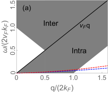
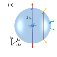
Figure 1: (a) Allowed energy-momentum regions of electron-hole pair excitations for a Weyl node, indicated as shaded areas. The dashed lines show the dispersion of the two circularly polarized phonon modes. The “intra” and “inter” denote intra-band and inter-band pairing, respectively. $k_{F}$ is the Fermi momentum of electrons. (b) Spin configurations of the initial and final states in transitions induced by phonons. We show three representative cases for different phonon wave vectors: a small one, an intermediate one, and the largest one allowing for the phonon absorption.

Next, we consider the damping of phonons in WSMs. We assume that the Weyl nodes are well separated in the reciprocal space: $k_{0}\gg k_{F}$, where $k_{F}$ is the Fermi wave number. We further limit our consideration to long-wave phonons with $|\bm{q}|\ll 2k_{0}$. As a result, all electron transitions induced by the phonons are within one of the Weyl nodes, and the Weyl nodes can be considered separately. The electron dispersion near a Weyl node consists of an upper band and a lower band separated by the band touching point. In principle, an electron absorbing a phonon could make either an intra-band transition or an inter-band transition. The possibility is constrained by the laws of energy and momentum conservation. Figure 1(a) shows the allowed momentum-energy regions in which phonons could excite an electron-hole pair and be absorbed. We find that a phonon can only induce the intra-band transition because the speed of sound is much smaller than the Fermi velocity in real materials.

We first determine the phonon damping for a single Weyl node. For a acoustic wave propagating along the magnetization axis ($z$-axis) with $q_{z}<2k_{F}-\omega/v_{F}$, we obtain supplementary :

$$\gamma_{\pm}^{D} =\gamma_{0}\left(\frac{\left|q_{z}\right|}{k_{F}}+\frac{1}{4}\frac{q_{z}^{2}\left|q_{z}\right|}{k_{F}^{3}}\right)+\mathcal{O}\left(\frac{c_{T}}{v_{F}}\right),$$ (9)

$$\gamma_{\pm}^{A} =\pm\eta\gamma_{0}\frac{q_{z}\left|q_{z}\right|}{k_{F}^{2}}+2\gamma_{0}\frac{q_{z}^{2}}{k_{F}^{2}}\frac{k_{F}}{k_{0}}\frac{c_{T}}{v_{F}}+\mathcal{O}\left(\frac{c_{T}^{2}}{v_{F}^{2}}\right),$$ (10)

where $\gamma_{0}\equiv(3/16)\pi\hbar\left(n_{e}/\rho_{I}\right)k_{0}^{2}$ with $n_{e}=k_{F}^{3}/3\pi^{2}$ being the electron number density and $\rho_{I}$ the ion mass density, the subscript “$\pm$” denotes the chirality of the Weyl node, and $\eta=\pm 1$ depending on whether the Fermi level of electrons is located in the upper band ($+1$) or the lower band ($-1$). $\gamma^{A}$ and $\gamma^{D}$ are both expanded in powers of $\omega$, which is substituted by $\omega_{q_{z},L/R}\approx c_{T}q_{z}$. We ignore the small splitting induced by the dissipationless viscosity because the contribution is of the higher order ($c_{T}\ll v_{F}$, $\Delta c_{T}\ll c_{T}$). For $q_{z}>2k_{F}-\omega/v_{F}$, the damping coefficients rapidly decay to zero.

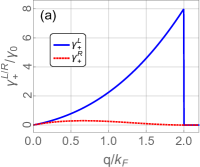
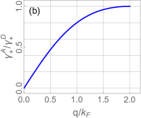
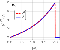
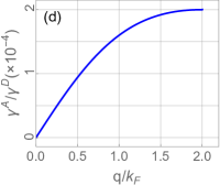
Figure 2: Damping coefficients for LCP ($\gamma^{L}$) and RCP ($\gamma^{R}$) phonon modes and the strengths of the circular dichroism $\gamma^{A}/\gamma^{D}$ versus the phonon wave number $q_{z}$ for a single left-handed ($+$) Weyl node (a, b) and a pair of Weyl nodes (c, d) in a $\mathcal{I}$ symmetric system with $k_{0}=10k_{F}$, $c_{T}=10^{-3}v_{F}$.

The phonon damping coefficient of a single left-handed ($+$) Weyl node is shown in Fig. 2(a, b). We find that the damping of the LCP phonons is much stronger than that of the RCP phonons. The relative circular dichroism $\gamma_{+}^{A}/\gamma_{+}^{D}$, shown in Fig. 2(b), is an increasing function of $q_{z}$, vanishing at $q_{z}=0$ and reaching a maximum of $100\%$ at $q_{z}=2k_{F}$. Because the energy of an electron is approximately conserved when absorbing a phonon, the initial and final states of the electron must be close to the Fermi surface. As a result, the selectivity is derived from the spin texture on the Fermi surface. It is maximized (minimized) when the spin directions of the initial and final states are anti-parallel (parallel) to each other, as shown by Fig. 1(b). For a single Weyl node of the right-handed chirality ($-$), the leading contribution in $\gamma^{A}$ will flip a sign. In this case, the damping of the RCP phonons will be stronger.

Because Weyl nodes always appear in pairs, we sum contributions from a pair of Weyl nodes of opposite chirality. In systems without breaking $\mathcal{I}$, the two Weyl nodes related by the symmetry are identical except the chirality. From Eq. (10), we find the total circular dichroism $\gamma^{A}=\gamma_{+}^{A}+\gamma_{-}^{A}=4\gamma_{0}(q_{z}/k_{F})^{2}(k_{F}/k_{0})(c_{T}/v_{F})$, with the leading contribution in $\gamma_{\pm}^{A}$ cancelled. It results in a strongly suppressed total circular dichroism. It is non-vanishing but tiny, as shown in Fig. 2 (c-d).

The circular phonon dichroism can be greatly enhanced by breaking $\mathcal{I}$ ($\lambda\neq 0$), which shifts the two Weyl nodes to different energies $\varepsilon^{\pm}=\mp\lambda$, as shown in the inset of Fig. 3. The effect is clearly manifested for the case of zero doping ($\mu=0$). In this case, the Fermi level is crossing the upper band ($\eta=1$) of one of the two Weyl nodes and the lower band ($\eta=-1$) of the other one, giving rise to an electron-like Fermi sphere and a hole-like Fermi sphere of the same sizes. As a result, from Eq. (10), the leading contributions in $\gamma_{\pm}^{A}$ are not canceling each other out but adding up, and the total circular dichroism $\gamma^{A}$ will be the double of that from a single node. For the more general cases of non-zero doping $(\mu\neq 0$), the sizes of the two Fermi spheres will be different with $k_{F}^{\pm}=(1/\hbar v_{F})\left|\lambda\pm\mu\right|$, and the Fermi spheres could become both electron-like (hole-like) when $|\mu/\lambda|\geq 1$. Figure 3 shows the total relative circular dichroism for different positions of the Fermi level. We find that the giant circular dichroism is gradually suppressed when the system moves away from the zero doping. The relative circular dichroism for $\mu\neq 0$ shows a sharp drop or rise at $q_{z}\approx 2k_{F}^{-}$ due to the vanishing of the contribution of the “$-$” Weyl node. In essence, the breaking of $\mathcal{I}$ unearths the giant circular dichroism inherent to each of the Weyl nodes.

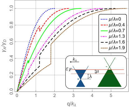
Figure 3: Relations of $\gamma_{A}/\gamma_{D}$ versus $q_{z}$ for different chemical potential $\mu$ when $\mathcal{I}$ is broken. $k_{\lambda}\equiv\lambda/\left(\hbar v_{F}\right)$. The discontinuity for the case of non-zero doping is due to the different sizes of the two Fermi spheres, and occurs at the maximal phonon absorption wave-number of the Weyl node with the smaller $k_{F}$.

Experimental realization.—The circular phonon dichroism can be detected by measuring the difference of the attenuation of the LCP/RCP acoustical waves in ultrasonic experiments. We can estimate the damping coefficients for a magnetic Weyl semimetal. We choose parameters $\rho_{I}\sim 5\ \text{g}/\text{$\text{cm}^{3}$}$, $n_{e}\sim 10^{17}\ \text{cm}^{-3}$, $k_{0}\sim 0.1\ \text{\r{A}}^{-1}$ and $c_{T}\sim 10^{3}\ \text{m}/\text{s}$, which are typical values for known magnetic WSMs and Dirac semimetals Hirschberger ; Liu ; Liu1 ; Jeon ; Xiong . We obtain $\gamma_{0}\sim 1.24\times 10^{3}\ \text{s}^{-1}$. At $q=2k_{F}$ when the circular dichroism maximizes, the difference of the attenuation for the LCP/RCP waves is the order of $\Delta\alpha=16\gamma_{0}/c_{T}\sim 20\,\text{m}^{-1}\approx 0.1\ \mathrm{dB/mm}$. An alternative detection is to inject a linearly polarized TA wave along a high symmetry magnetization axis. Due to the different phonon damping rates of the LCP and RCP modes, the linearly polarized wave will gradually become elliptically polarized and finally circularly polarized. The presence of the dissipationless viscosity will also induce a rotation of the major axis of the ellipse of the polarization. The latter is the counterpart of the acoustic Faraday rotation observed in magnetic insulators Sytcheva . The effect may find practical applications. For instance, WSMs breaking both $\mathcal{T}$ and $\mathcal{I}$ can be used as acoustic polarizers, which generate circularly polarized acoustic waves from linearly polarized sources.

Summary and Discussion.—In summary, we have shown that in magnetic metals with strong SOC, both the dissipationless viscosity and the dissipative viscosity emerge. In particular, the dissipative viscosity will induce the circular phonon dichroism. It offers a new degree of manipulation of phonons, i.e., the control of the phonon polarization. We further show that WSMs breaking both $\mathcal{T}$ and $\mathcal{I}$ exhibit giant circular phonon dichroism, which provides a new characterization to these topologically nontrivial materials and may find practical applications.

Our study of the circular phonon dichroism in Weyl semimetals is limited to the long-wave acoustic phonons. We note that the same effect also presents for short-wave acoustic phonons as well as optical phonons. The general formalism we have developed provides a solid foundation and a unified approach for the calculation of the effect in real materials. We further note that similar effects had been predicted in different contexts in literatures. For instance, the Zeeman splitting of optical phonons in multiferroic materials predicted in Ref. Dynamical Multiferroicity is actually a manifestation of the dissipationless viscosity in the optical branch of phonons.

Supplementary Materials for “Circular Phonon Dichroism in Weyl Semimetals”

I Dissipationless viscosity in an insulator

In the main text, we generalize the definition of the dissipationless viscosity. Here, we show that $G_{\alpha\beta}$ defined in the main text is exactly the effective magnetic field for phonons defined in Ref. Qin for an insulator. We note that in the total Hamiltonian $\hat{H}$ of the electron system, only $\hat{V}_{ei}$ depends on the ion displacement $\bm{u}_{i}$. As a result, we can rewrite the response function Eq. (3) as:

$$\mathcal{G}_{\alpha\beta}^{R}\left(\boldsymbol{R}_{n}-\boldsymbol{R}_{n^{\prime}},t-t^{\prime}\right)=-\frac{i}{\hbar}\theta\left(t-t^{\prime}\right)\left\langle\left[\frac{\partial\hat{H}}{\partial u_{n}^{\alpha}}\left(t\right),\frac{\partial\hat{H}}{\partial u_{n^{\prime}}^{\beta}}\left(t^{\prime}\right)\right]\right\rangle_{0}.$$ (S1)

$\mathcal{G}_{\alpha\beta}^{R}$ can be expressed in the Lehmann representation at zero temperature:

$$\mathcal{G}_{\alpha\beta}^{R}\left(\boldsymbol{R}_{n}-\boldsymbol{R}_{n^{\prime}},\omega\right)= \sum_{m\neq 0}\frac{\left\langle\Phi_{0}\right|\frac{\partial\hat{H}}{\partial u_{n}^{\alpha}}\left|\Phi_{m}\right\rangle\left\langle\Phi_{m}\right|\frac{\partial\hat{H}}{\partial u_{n^{\prime}}^{\beta}}\left|\Phi_{0}\right\rangle}{\hbar\omega+\epsilon_{0}-\epsilon_{m}+i\varepsilon}-\frac{\left\langle\Phi_{0}\right|\frac{\partial\hat{H}}{\partial u_{n^{\prime}}^{\beta}}\left|\Phi_{m}\right\rangle\left\langle\Phi_{m}\right|\frac{\partial\hat{H}}{\partial u_{n}^{\alpha}}\left|\Phi_{0}\right\rangle}{\hbar\omega-\epsilon_{0}+\epsilon_{m}+i\varepsilon},$$ (S2)

where $\left|\Phi_{m}\right\rangle$ denotes an eigenstate with an energy $\epsilon_{m}$ , and $\left|\Phi_{0}\right\rangle$ the ground state. For an insulator, there is a gap separating the ground state from the excited states, $\epsilon_{m}-\epsilon_{0}>0$ ($m\neq 0$). In this case, the dissipative (anti-hermitian) part of response function vanishes, and the infinitesimal factor $i\varepsilon$ can be neglected in Eq. (S2). Following the definition shown in the main text, we have:

$$G_{\alpha\beta}\left(\boldsymbol{R}_{n}-\boldsymbol{R}_{n^{\prime}}\right)=-i\frac{d\mathcal{G}_{\alpha\beta}^{R}\left(\boldsymbol{R}_{n}-\boldsymbol{R}_{n^{\prime}},\omega\right)}{d\omega}\mid_{\omega\rightarrow 0}.$$ (S3)

We obtain:

$$G_{\alpha\beta}\left(\boldsymbol{R}_{n}-\boldsymbol{R}_{n^{\prime}}\right)=i\hbar\sum_{m\neq 0}\frac{\left\langle\Phi_{0}\right|\frac{\partial H}{\partial u_{n}^{\alpha}}\left|\Phi_{m}\right\rangle\left\langle\Phi_{m}\right|\frac{\partial H}{\partial u_{n^{\prime}}^{\beta}}\left|\Phi_{0}\right\rangle-\left\langle\Phi_{0}\right|\frac{\partial H}{\partial u_{n^{\prime}}^{\beta}}\left|\Phi_{m}\right\rangle\left\langle\Phi_{m}\right|\frac{\partial H}{\partial u_{n}^{\alpha}}\left|\Phi_{0}\right\rangle}{\left(\epsilon_{0}-\epsilon_{m}\right)^{2}}.$$ (S4)

Note that the adiabatic wave function $\Phi_{m}$ depends on parameters $\{\boldsymbol{u}\}$ (or $\{\boldsymbol{R}\}$).

To simplify, we employ identities:

$$\left\langle\left.\frac{\partial\Phi_{l}}{\partial u_{n}^{\alpha}}\right|\Phi_{m}\right\rangle =\frac{\left\langle\Phi_{l}\left|\frac{\partial\hat{H}}{\partial u_{n}^{\alpha}}\right|\psi_{m}\right\rangle}{\epsilon_{l}-\epsilon_{m}},$$ (S5)

$$\left\langle\Phi_{l}\left|\frac{\partial\Phi_{m}}{\partial u_{n}^{\alpha}}\right.\right\rangle =\frac{\left\langle\Phi_{l}\left|\frac{\partial\hat{H}}{\partial u_{n}^{\alpha}}\right|\Phi_{m}\right\rangle}{\epsilon_{m}-\epsilon_{l}},$$ (S6)

for $l\neq m$. We have:

$$G_{\alpha\beta}\left(\boldsymbol{R}_{n}-\boldsymbol{R}_{n^{\prime}}\right)=i\hbar\sum_{m}\left(\left\langle\left.\frac{\partial\Phi_{0}}{\partial u_{n}^{\alpha}}\right|\Phi_{m}\right\rangle\left\langle\Phi_{m}\left|\frac{\partial\Phi_{0}}{\partial u_{n^{\prime}}^{\beta}}\right.\right\rangle-\left\langle\left.\frac{\partial\Phi_{0}}{\partial u_{n^{\prime}}^{\beta}}\right|\Phi_{m}\right\rangle\left\langle\Phi_{m}\left|\frac{\partial}{\partial u_{n}^{\alpha}}\Phi_{0}\right.\right\rangle\right).$$ (S7)

Noting $\sum_{m}\left|\Phi_{m}\right\rangle\left\langle\Phi_{m}\right|=1$, we obtain:

$$G_{\alpha\beta}\left(\boldsymbol{R}_{n}-\boldsymbol{R}_{n^{\prime}}\right)=2\hbar\mbox{Im}\left\langle\left.\frac{\partial\Phi_{0}}{\partial u_{n^{\prime}}^{\beta}}\right|\frac{\partial\Phi_{0}}{\partial u_{n}^{\alpha}}\right\rangle.$$

This is exactly the effective magnetic field for phonons defined in Ref. Qin .

II Viscosity coefficients of a non-interacting system

In this section, we derive the viscosity coefficients for a non-interacting system.

For a non-interacting system, Eq. (S1) can be written as:

$$\mathcal{G}_{\alpha\beta}^{R}\left(\boldsymbol{q},\omega\right)=\frac{1}{M}\sum_{\boldsymbol{k}\boldsymbol{k}^{\prime}ss^{\prime}}\left\langle\psi_{\boldsymbol{k}s}\left|\frac{\partial\hat{v}}{\partial u_{-\boldsymbol{q}}^{\alpha}}\right|\psi_{\boldsymbol{k}^{\prime}s^{\prime}}\right\rangle\left\langle\psi_{\boldsymbol{k}^{\prime}s^{\prime}}\left|\frac{\partial\hat{v}}{\partial u_{\boldsymbol{q}}^{\beta}}\right|\psi_{\boldsymbol{k}s}\right\rangle\frac{f_{\boldsymbol{k}s}-f_{\boldsymbol{k}^{\prime}s^{\prime}}}{\epsilon_{\boldsymbol{k}s}-\epsilon_{\boldsymbol{k}^{\prime}s^{\prime}}+\hbar\omega+i\varepsilon},$$ (S8)

where $\hat{v}(\bm{r})=\sum_{\bm{R}}v_{ei}(\bm{r}-\bm{R})$ is the single-particle interacting energy between an electron and all ions, $\psi_{\boldsymbol{k}s}$ is the Bloch wave function at $\bm{k}$ and band $s$ with $\psi_{\boldsymbol{k}s}\left(\boldsymbol{r}\right)=N^{-1/2}e^{i\boldsymbol{k}\cdot\boldsymbol{r}}u_{{\boldsymbol{k}s}}\left(\boldsymbol{r}\right)$, $\epsilon_{\boldsymbol{k}s}$ is the electron dispersion, and $\partial\hat{v}/\partial u_{\boldsymbol{q}}^{\alpha}$ is the Fourier transform of $\partial\hat{v}/\partial u_{n}^{\alpha}$:

$$\frac{\partial\hat{v}}{\partial u_{\boldsymbol{q}}^{\alpha}}=\frac{1}{\sqrt{N}}\sum_{n}\left(\frac{\partial\hat{v}}{\partial u_{n}^{\alpha}}\right)_{\{\boldsymbol{u}_{n}\}=0}e^{i\boldsymbol{q}\cdot\boldsymbol{R}_{n}^{0}}\equiv\frac{1}{2\sqrt{N}}\{\hat{T}_{\bm{q},\alpha},\,e^{i\bm{q}\cdot\bm{r}}\},$$ (S9)

where $\{\hat{T}_{\bm{q}},\,e^{i\bm{q}\cdot\bm{r}}\}$ denotes the anti-commutator of the two operators.

By substituting Eq. (S9) into Eq. (S8), we obtain:

$$\mathcal{G}_{\alpha\beta}\left(\boldsymbol{q},\omega\right)=\frac{1}{MN}\sum_{\boldsymbol{k}ss^{\prime}}\left\langle u_{\boldsymbol{k}s}\left|\hat{T}_{\bm{k},\bm{k}+\boldsymbol{q}}^{\alpha}\right|u_{\boldsymbol{k}+\boldsymbol{q}s^{\prime}}\right\rangle\left\langle u_{\boldsymbol{k}+\boldsymbol{q}s^{\prime}}\left|\hat{T}_{\bm{k}+\bm{q},\boldsymbol{k}}^{\beta}\right|u_{\boldsymbol{k}s}\right\rangle\frac{f_{\boldsymbol{k}s}-f_{\boldsymbol{k}+\boldsymbol{q}s^{\prime}}}{\epsilon_{\boldsymbol{k}s}-\epsilon_{\boldsymbol{k}+\boldsymbol{q}s^{\prime}}+\hbar\omega+i\varepsilon},$$ (S10)

where

$$\hat{T}_{\bm{k},\bm{k}^{\prime}}^{\alpha}=\frac{1}{2}\left(e^{-i\bm{k}\cdot\bm{r}}\hat{T}_{\bm{k}-\bm{k}^{\prime},\alpha}e^{i\bm{k}\cdot\bm{r}}+e^{-i\bm{k}^{\prime}\cdot\bm{r}}\hat{T}_{\bm{k}-\bm{k}^{\prime},\alpha}e^{i\bm{k}^{\prime}\cdot\bm{r}}\right),$$ (S11)

Using the definitions of the viscosity coefficients:

$$G_{\alpha\beta}\left(\boldsymbol{q}\right) =-\frac{i}{2}\lim_{\omega\rightarrow 0}\frac{d}{d\omega}\left(\mathcal{G}_{\alpha\beta}^{R}+\mathcal{G}_{\alpha\beta}^{R*}\right),$$ (S12)

$$\gamma_{\alpha\beta}\left(\boldsymbol{q},\omega\right) =\frac{i}{4\omega}\left(\mathcal{G}_{\alpha\beta}^{R}-\mathcal{G}_{\alpha\beta}^{R*}\right),$$ (S13)

we obtain their explicit forms:

$$G_{\alpha\beta} =\frac{i\hbar}{MN}\sum_{ss^{\prime}\boldsymbol{k}}\left(f_{\boldsymbol{k}s}-f_{\boldsymbol{k}+\boldsymbol{q}s^{\prime}}\right)\frac{\left\langle\varphi_{\boldsymbol{k}s}\right|\mathnormal{\hat{T}_{\bm{k},\bm{k}+\boldsymbol{q}}^{\alpha}}\left|\varphi_{\boldsymbol{k}+\boldsymbol{q}s^{\prime}}\right\rangle\left\langle\varphi_{\boldsymbol{k}+\boldsymbol{q}s^{\prime}}\right|\hat{T}_{\bm{k}+\bm{q},\boldsymbol{k}}^{\beta}\left|\varphi_{\boldsymbol{k}s}\right\rangle}{\left(\epsilon_{\boldsymbol{k}s}-\epsilon_{\boldsymbol{k}+\boldsymbol{q}s^{\prime}}\right)^{2}+\varepsilon^{2}},$$ (S14)

$$\gamma_{\alpha\beta} =\frac{\pi}{2MN\omega}\sum_{ss^{\prime}\boldsymbol{k}}\left(f_{\boldsymbol{k}s}-f_{\boldsymbol{k}+\boldsymbol{q}s^{\prime}}\right)\delta\left(\epsilon_{\boldsymbol{k}s}-\epsilon_{\boldsymbol{k}+\boldsymbol{q}s^{\prime}}+\hbar\omega\right)\left\langle\varphi_{\boldsymbol{k}s}\right|\hat{T}_{\bm{k},\bm{k}+\boldsymbol{q}}^{\alpha}\left|\varphi_{\boldsymbol{k}+\boldsymbol{q}s^{\prime}}\right\rangle\left\langle\varphi_{\boldsymbol{k}+\boldsymbol{q}s^{\prime}}\right|\hat{T}_{\bm{k}+\bm{q},\boldsymbol{k}}^{\beta}\left|\varphi_{\boldsymbol{k}s}\right\rangle.$$ (S15)

III Kramer-Kronig relation

Because both the dissipationless and the dissipative viscosities are derived from the retarded response function $\mathcal{G}_{\alpha\beta}^{R}\left(\omega\right)$, they are inherently related. To see that, we make use of the Kramers-Kronig relation of $\mathcal{G}_{\alpha\beta}^{R}\left(\omega\right)$S (1):

$$\mathcal{G}_{\alpha\beta}^{R}\left(\bm{q},\omega\right)=-i\mathcal{P}\int_{-\infty}^{+\infty}\frac{\mathcal{G}_{\alpha\beta}^{R}\left(\bm{q},\nu\right)}{\nu-\omega}\frac{d\nu}{\pi},$$ (S16)

where $\mathcal{P}$ denotes the Cauchy principal value. Substituting Eq. (S16) into Eq. (S12) and making use Eq. (S13), we obtain

$$G_{\alpha\beta}(\bm{q}) =-\frac{i}{2}\lim_{\omega\rightarrow 0}\frac{d}{d\omega}\left[-i\mathcal{P}\int_{-\infty}^{+\infty}\frac{\mathcal{G}_{\alpha\beta}^{R}\left(\bm{q},\nu\right)-\mathcal{G}_{\beta\alpha}^{R*}\left(\bm{q},\nu\right)}{\nu-\omega}\frac{d\nu}{\pi}\right]$$

$$=-2\lim_{\omega\rightarrow 0}\frac{d}{d\omega}\left[-i\mathcal{P}\int_{-\infty}^{+\infty}\frac{\nu\gamma_{\alpha\beta}\left(\bm{q},\nu\right)}{\nu-\omega}\frac{d\nu}{\pi}\right]$$

$$=2i\mathcal{P}\int_{-\infty}^{+\infty}\frac{\gamma_{\alpha\beta}\left(\bm{q},\nu\right)}{\nu}\frac{d\nu}{\pi}.$$ (S17)

The positive frequency and the negative frequency components of the $\gamma$ coefficients are related S (1):

$$\gamma_{\alpha\beta}\left(\boldsymbol{q},-\omega\right)=\gamma_{\beta\alpha}\left(-\boldsymbol{q},\omega\right).$$ (S18)

We obtain Eq. (6) by substituting Eq. (S18) into (S17).

IV the dissipationless viscosity of a deformation-dependent Haldane Model

We study a Haldane Model S (2) which is coupled to the lattice deformation by

$$H=\epsilon\left(k\right)+d_{i}\left(k\right)e_{a}^{i}\sigma^{a},$$ (S19)

where $\epsilon\left(\boldsymbol{k}\right)=2t_{2}\cos\phi\sum_{i}\cos\left(\boldsymbol{k}\cdot\boldsymbol{b}_{i}\right)$, $d_{x}\left(\boldsymbol{k}\right)=t_{1}\sum_{i}\cos\left(\boldsymbol{k}\cdot\boldsymbol{a}_{i}\right)$, $d_{y}\left(\boldsymbol{k}\right)=t_{1}\sum_{i}\sin\left(\boldsymbol{k}\cdot\boldsymbol{a}_{i}\right)$, $d_{z}\left(\boldsymbol{k}\right)=\epsilon_{0}-2t_{2}\sin\phi\left(\sum_{i}\sin\left(\boldsymbol{k}\cdot\boldsymbol{b}_{i}\right)\right)$, $i=1,2,3$, $\boldsymbol{a}_{i}$ and $\boldsymbol{b}_{i}$ are vectors connecting nearest and second- nearest sites, $t_{1}$ and $t_{2}\exp(i\phi)$ are the hopping constants of the nearest and next-nearest neighbors, $\epsilon_{0}$ is the on-site energy ($+\epsilon_{0}$ and $-\epsilon_{0}$ for two sub-lattices). The lattice constant is $a$. For $\left|t_{2}/t_{1}\right|<1/3$, the Chern number is non-zero when $\left|\epsilon_{0}/t_{2}\right|<3\sqrt{3}\left|\sin\phi\right|$.

We set $\phi=\pi/2$, and calculate the dissipationless viscosity. The relation of the dissipationless viscosity and parameter $\epsilon_{0}$ for different $t_{2}$ is shown in Fig. S1. It shows that the dissipationless viscosity is nonzero even when the Chern number is zero, although there appears a kink at the point of the transition from a topologically nontrivial regime to a trivial one.

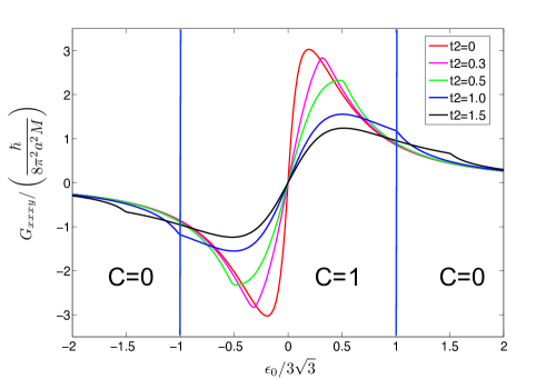
Figure S1: The dissipationless viscosity of a Haldane model coupling with lattice deformation.

In Fig. S1, $G_{xxxy}$ is defined as

$$G_{xxxy}=\frac{1}{2}\lim_{\bm{q}\rightarrow 0}\frac{\partial^{2}}{\partial q_{x}^{2}}G_{xy},$$ (S20)

and can be calculated by:

$$G_{xxxy}=\frac{1}{MV}\frac{d}{d\omega}\int_{-\infty}^{+\infty}dte^{i\omega t}\left[-\frac{i}{\hbar}\theta\left(t-t^{\prime}\right)\right]\left\langle\left[\frac{\partial H}{\partial e_{x}^{x}}\left(t\right),\frac{\partial H}{\partial e_{y}^{x}}\right]\right\rangle_{0}.$$ (S21)

V Circular phonon dichroism of a single Weyl node

We first consider a left-handed Weyl node. The eigenstates of the low energy effective Hamiltonian Eq. (8) in the absence of the lattice deformation can be written as $\psi_{\eta,\boldsymbol{k}}\left(\boldsymbol{r}\right)=V^{-\frac{1}{2}}e^{i\boldsymbol{k}\cdot\boldsymbol{r}}\chi_{\eta,\tilde{\boldsymbol{k}}}$ with $\eta=\pm$ denoting the upper and the lower band, respectively, $\tilde{\boldsymbol{k}}\equiv\boldsymbol{k}-k_{0}\hat{z}$ , and

$$\chi_{+,\tilde{\boldsymbol{k}}} =\left(\begin{array}[]{c}\cos\frac{\theta_{\tilde{\bm{k}}}}{2}\\ \sin\frac{\theta_{\tilde{\bm{k}}}}{2}e^{i\varphi_{\tilde{\bm{k}}}}\end{array}\right),$$ (S24)

$$\chi_{-,\tilde{\boldsymbol{k}}} =\left(\begin{array}[]{c}-\sin\frac{\theta_{\tilde{\bm{k}}}}{2}e^{-i\varphi_{\tilde{\bm{k}}}}\\ \cos\frac{\theta_{\tilde{\bm{k}}}}{2}\end{array}\right),$$ (S27)

where $\theta_{\tilde{\bm{k}}}$ and $\varphi_{\tilde{\bm{k}}}$ are the polar and azimuthal angles of the vector $\tilde{\boldsymbol{k}}$. The corresponding eigen-energies are $\varepsilon_{\boldsymbol{k}\eta}=\eta\hbar v_{F}\left|\tilde{\boldsymbol{k}}\right|$.

Using the definition Eq. (S11) and the effective Hamiltonian Eq. (8), we obtain:

$$\hat{T}_{\bm{k},\boldsymbol{k}^{\prime}}^{\alpha}=\frac{i\hbar v_{F}}{2}\left(\bm{k}-\bm{k}^{\prime}\right)\cdot\left(\bm{k}+\bm{k}^{\prime}\right)\hat{\sigma}^{\alpha}.$$ (S28)

Here, we have set $N=V$ when applying Eq. (S11). It is a convenient choice for a continuous system defined by Eq. (8).

We have shown in the main text that phonons can only induce the intra-band transition in a Weyl node. Only the term with $s=s^{\prime}=\eta$ in Eq. (7) is contributing to $\gamma_{\alpha\beta}$. By substituting Eq. (S28) into Eq. (S15), we obtain:

$$\gamma_{\alpha\beta}^{+}\left(\boldsymbol{q},\tilde{\omega}\right)=\frac{\pi\hbar}{2\tilde{\omega}M}\int\frac{dk^{3}}{\left(2\pi\right)^{3}}F_{\eta}^{\alpha\beta}\left(\tilde{\boldsymbol{k}},\tilde{\boldsymbol{k}}^{\prime}\right)\left[\boldsymbol{q}\cdot\left(\boldsymbol{k}+\frac{\boldsymbol{q}}{2}\right)\right]^{2}\left(f_{\boldsymbol{k}\eta}-f_{\boldsymbol{k}+\boldsymbol{q}\eta}\right)\delta\left(\tilde{\omega}+\eta\left|\tilde{\boldsymbol{k}}\right|-\eta\left|\tilde{\boldsymbol{k}}+\boldsymbol{q}\right|\right),$$ (S29)

where the superscript “$+$” denotes the left-handed chirality of Weyl node, $\tilde{\omega}=\omega/v_{F}$, and

$$F_{\eta}^{\alpha\beta}\left(\tilde{\boldsymbol{k}},\tilde{\boldsymbol{k}}^{\prime}\right)=\left\langle\chi_{\eta,\tilde{\boldsymbol{k}}}\right|\hat{\sigma}^{\alpha}\left|\chi_{\eta,\tilde{\boldsymbol{k}}+\boldsymbol{q}}\right\rangle\left\langle\chi_{\eta,\tilde{\boldsymbol{k}}+\boldsymbol{q}}\right|\hat{\sigma}^{\beta}\left|\chi_{\eta,\tilde{\boldsymbol{k}}}\right\rangle.$$ (S30)

It is straightforward to evaluate the matrix elements and obtain :

$$F_{\eta}^{xy}\left(\boldsymbol{k};\boldsymbol{k}^{\prime}\right) =\frac{i\eta\left(k_{z}k^{\prime}-kk_{z}^{\prime}\right)+k_{x}k_{y}^{\prime}+k_{y}k_{x}^{\prime}}{2kk^{\prime}},$$ (S31)

$$F_{\eta}^{xx}\left(\boldsymbol{k},\boldsymbol{k}^{\prime}\right) =\frac{kk^{\prime}-k_{z}k_{z}^{\prime}-k_{y}k_{y}^{\prime}+k_{x}k_{x}^{\prime}}{2kk^{\prime}}.$$ (S32)

Completing the integral, we obtain the full expression for the damping coefficients for phonons with $\bm{q}=(0,0,q_{z})$,

$$\gamma_{xy}^{+} =-i\gamma_{0}\mbox{sign}\left(q_{z}\right)\frac{\left(q_{z}^{2}-\tilde{\omega}^{2}\right)}{k_{F}^{2}}\left(\eta+\frac{2k_{F}\tilde{\omega}}{k_{0}q_{z}}+\eta\frac{k_{F}^{2}\tilde{\omega}^{2}}{k_{0}^{2}q_{z}^{2}}+\frac{\tilde{\omega}^{3}}{6k_{F}k_{0}q_{z}}+\eta\frac{\tilde{\omega}^{4}}{4k_{0}^{2}q_{z}^{2}}\right),$$ (S33)

$$\gamma_{xx}^{+} =\gamma_{0}\mbox{sign}\left(q_{z}\right)\frac{\left(q_{z}^{2}-\tilde{\omega}^{2}\right)}{k_{F}^{2}}\left[\left(\frac{k_{F}}{q_{z}}+\frac{q_{z}}{4k_{F}}\right)+\eta\left(\frac{2k_{F}^{2}}{k_{0}q_{z}^{2}}+\frac{1}{2k_{0}}\right)\tilde{\omega}+\left(\frac{k_{F}^{3}}{k_{0}^{2}q_{z}^{3}}+\frac{k_{F}}{4k_{0}^{2}q_{z}}+\frac{1}{12k_{F}q_{z}}\right)\tilde{\omega}^{2}+\eta\frac{\tilde{\omega}^{3}}{2k_{0}q_{z}^{2}}\right.$$

$$\left.+\left(\frac{k_{F}}{2k_{0}^{2}q_{z}^{3}}+\frac{1}{48k_{F}k_{0}^{2}q_{z}}\right)\tilde{\omega}^{4}+\frac{\tilde{\omega}^{6}}{80k_{F}k_{0}^{2}q_{z}^{3}}\right],$$ (S34)

where $\gamma{}_{0}=\frac{3}{16}\pi\hbar\left(n_{e}/\rho_{I}\right)k_{0}^{2}$, and the formulas are valid only when $|q_{z}|<2k_{F}-\tilde{\omega}$. The damping coefficients vanishes when $|q_{z}|>2k_{F}+\tilde{\omega}$. In the intermediate regime $2k_{F}-\tilde{\omega}<|q_{z}|<2k_{F}+\tilde{\omega}$, the damping coefficients rapidly decay to zero.

Because the left- and right-handed Weyl nodes can be related to each other by $\mathcal{I}$ , the damping coefficients of a right handed Weyl node can be obtained by the relation $\gamma_{\alpha\beta}^{-}\left(\boldsymbol{q}\right)=\gamma_{\alpha\beta}^{+}\left(-\boldsymbol{q}\right)$.

For the long-wave TA phonon with the dispersion $\omega=c_{T}q_{z}$, $\tilde{\omega}_{q_{z},L/R}=\left(c_{T}/v_{F}\right)q_{z}$ is a small quantity since $c_{T}\ll v_{F}$. By keeping the leading order terms in Eq. (S33) and (S34), we obtain Eqs. (9,10).

VI Elastic gauge field

In Eq. (8), we only consider the minimum coupling between electrons and the lattice deformation. An alternative way to introduce the coupling is through an elastic gauge field. For the elastic gauge field, we adopt the effective Hamiltonian obtained in Ref. Cortijo :

$$H=\boldsymbol{\sigma}\cdot\left(\hbar v_{F}\boldsymbol{k}_{\perp}\pm\boldsymbol{A}_{\perp}\right)\mp\sigma_{z}\left(\hbar v_{F}k_{z}\pm A_{z}\right),$$ (S35)

where we assume that the Fermi velocity is isotropic. The elastic gauge fields are expressed as, in our notation:

$$A_{x}^{el} =\beta b_{3}u_{zx},$$ (S36)

$$A_{y}^{el} =\beta b_{3}u_{zy},$$ (S37)

$$A_{z}^{el}= 2\beta b_{3}u_{zz}-\sum_{j}\beta ru_{jj},$$ (S38)

where $u_{ij}$ is the strain tensor, and $\beta$ is the Grüneisen parameter Shapourian . In tight-binding models, $\beta$ is defined as $\beta=-\partial\ln t/\partial\ln a\simeq 2$, where $t$ and $a$ are the hopping integral and the distance between two sites, respectively.

Following the same procedure as shown in Sec. V, we obtain the leading contributions of the elastic gauge field:

$$\gamma_{\pm}^{D} =\gamma^{\prime}_{0}\left(\frac{\left|q_{z}\right|}{k_{F}}+\frac{1}{4}\frac{q_{z}^{2}\left|q_{z}\right|}{k_{F}^{3}}\right)+\mathcal{O}\left(\frac{c_{T}^{2}}{v_{F}^{2}}\right),$$ (S39)

$$\gamma_{\pm}^{A} =\pm\eta\gamma^{\prime}_{0}\frac{q_{z}\left|q_{z}\right|}{k_{F}^{2}}+\mathcal{O}\left(\frac{c_{T}^{2}}{v_{F}^{2}}\right).$$ (S40)

Compared with Eq. (9) and (10), $\gamma_{0}$ is changed to $\gamma^{\prime}_{0}=(\beta^{2}/4)\gamma_{0}$, scaled by a factor $\beta^{2}/4$. Since $\beta\simeq 2$, the elastic gauge field yields essentially the same result as that from the minimum coupling.

References

• (1) M. Maldovan, Nature (London) 503, 209 (2013).
• (2) N. B. Li, J. Ren, L. Wang, G. Zhang, P. Hänggi, and B. W. Li, Rev. Mod. Phys. 84, 1045 (2012).
• (3) B. Liang, B. Yuan, and J. C. Cheng, Phys. Rev. Lett. 103, 104301 (2009).
• (4) B. Liang, X. S. Guo, J. Tu, D. Zhang and J. C. Cheng, Nat. Mater. 9, 989 (2010).
• (5) X.-F. Li, X. Ni, L. Feng, M.-H. Lu, C. He, and Y.-F. Chen, Phys. Rev. Lett. 106, 084301 (2011).
• (6) N. Boechler, G. Theocharis, and C. Daraio, Nat. Mater. 10, 665 (2011).
• (7) M. Z. Hasan and C. L. Kane, Rev. Mod. Phys. 82, 3045 (2010).
• (8) X. L. Qi and S. C. Zhang, Rev. Mod. Phys. 83, 1057 (2011).
• (9) S. Jia, S.-Y. Xu, and M. Z. Hasan, Nat. Mater. 15, 1140 (2016).
• (10) L. Zhang, J. Ren, J.-S. Wang, and B. Li, Phys. Rev. Lett. 105, 225901 (2010).
• (11) R. Süsstrunk and S. D. Huber, Science 349, 47 (2015).
• (12) C. He, X. Ni, H. Ge, X.-C. Sun, Y.-B. Chen, M.-H. Lu, X.-P. Liu, and Y.-F. Chen, Nat. Phys. 12, 1124 (2016).
• (13) R. Fleury, D. L. Sounas, C. F. Sieck, M. R. Haberman, and A. Alù, Science 343, 516 (2014).
• (14) Z. Yang, F. Gao, X. Shi, X. Lin, Z. Gao, Y. Chong, and B. Zhang, Phys. Rev. Lett. 114, 114301 (2015).
• (15) X. Ni, C. He, X.-C. Sun, X.-p. Liu, M.-H. Lu, L. Feng, and Y.-F. Chen, New J. Phys. 17, 053016 (2015).
• (16) A. B. Khanikaev, R. Fleury, S. Hossein Mousavi, and A. Alù, Nat. Commun. 6, 8260 (2015).
• (17) P. Wang, L. Lu, and K. Bertoldi, Phys. Rev. Lett. 115, 104302 (2015).
• (18) M. Xiao, W. Chen, W. He, and C. T. Chan, Nat. Phys. 11, 920 (2015).
• (19) C. Strohm, G. L. J. A. Rikken, and P. Wyder, Phys. Rev. Lett. 95, 155901 (2005).
• (20) A. V. Inyushkin, and A. N. Taldenkov, JETP Lett. 86, 379 (2007).
• (21) T. Qin, J. H. Zhou, and J. R. Shi, Phys. Rev. B 86, 104305 (2012).
• (22) C. Hoyos and D. T. Son, Phys. Rev. Lett. 108, 066805 (2012).
• (23) T. L. Hughes, R. G. Leigh, and E. Fradkin, Phys. Rev. Lett. 107, 075502 (2011).
• (24) T. L. Hughes, R. G. Leigh, and O. Parrikar, Phys. Rev. D 88, 025040 (2013).
• (25) M. Barkeshli, S. B. Chung, and X. L. Qi, Phys. Rev. B 85, 245107 (2012).
• (26) H. Shapourian, T. L. Hughes, and S. Ryu, Phys. Rev. B 92, 165131 (2015).
• (27) L. Zhang and Q. Niu, Phys. Rev. Lett. 112, 085503 (2014).
• (28) L. Zhang and Q. Niu, Phys. Rev. Lett. 115, 115502 (2015).
• (29) S.-Y. Chen, C. Zheng, M. S. Fuhrer, and J. Yan, Nano Lett. 15, 2526 (2015).
• (30) G. D. Mahan, Many-particle physics, Third Edition (Kluwer Academic, 2000).
• (31) I. Errea, M. Calandra, and F. Mauri, Phys. Rev. Lett. 111, 177002 (2013).
• (32) M. Borinaga, I. Errea, M. Calandra, F. Mauri, and A. Bergara, Phys. Rev. B 93, 174308 (2016).
• (33) See Supplemental Materials.
• (34) A. A. Zyuzin, S. Wu, and A. A. Burkov, Phys. Rev. B 85, 165110 (2012).
• (35) A. Cortijo, Y. Ferreirós, K. Landsteiner, and M. A. H. Vozmediano, Phys. Rev. Lett. 115, 177202 (2015).
• (36) M. Hirschberger, S. Kushwaha, Z. Wang, Q. Gibson, S. Liang, C. A. Belvin, B. A. Bernevig, R. J. Cava, and N. P. Ong, Nat. Mater. 15, 1161 (2016).
• (37) Z. K. Liu, J. Jiang, B. Zhou, Z. J. Wang, Y. Zhang, H. M. Weng, D. Prabhakaran, S-K. Mo, H. Peng, P. Dudin, T. Kim, M. Hoesch, Z. Fang, X. Dai, Z. X. Shen, D. L. Feng, Z. Hussain, and Y. L. Chen, Nat. Mater. 13, 677 (2014).
• (38) S. Jeon, B. B. Zhou, A. Gyenis, B. E. Feldman, I. Kimchi, A. C. Potter, Q. D. Gibson, R. J. Cava, A. Vishwanath, and A. Yazdani, Nat. Mater. 13, 851 (2014).
• (39) Z. K. Liu, B. Zhou, Y. Zhang, Z. J. Wang, H. M. Weng, D. Prabhakaran, S.-K. Mo, Z. X. Shen, Z. Fang, X. Dai, Z. Hussain, Y. L. Chen, Science 343, 864 (2014).
• (40) J. Xiong, S. K. Kushwaha, T. Liang, J. W. Krizan, M. Hirschberger, W. Wang, R. J. Cava, and N. P. Ong, Science 350, 413 (2015).
• (41) A. Sytcheva, U. Löw, S. Yasin, J. Wosnitza, S. Zherlitsyn, P. Thalmeier, T. Goto, P. Wyder, and B. Lüthi, Phys. Rev. B 81, 214415 (2010).
• (42) D. M. Juraschek, M. Fechner, A. V. Balatsky and N. A. Spaldin, arXiv:1612.06331 (2016).

References

• S (1) G. Giuliani, and G. Vignale, Quantum Theory of the Electron Liquid, First Edition (Cambridge University Press, 2005).
• S (2) F. D. M. Haldane, Phys. Rev. Lett. 61, 2015 (1988).