Low Rank Independence Samplers in Bayesian Inverse Problems

Abstract

In Bayesian inverse problems, the posterior distribution is used to quantify uncertainty about the reconstructed solution. In practice, Markov chain Monte Carlo algorithms often are used to draw samples from the posterior distribution. However, implementations of such algorithms can be computationally expensive. We present a computationally efficient scheme for sampling high-dimensional Gaussian distributions in ill-posed Bayesian linear inverse problems. Our approach uses Metropolis-Hastings independence sampling with a proposal distribution based on a low-rank approximation of the prior-preconditioned Hessian. We show the dependence of the acceptance rate on the number of eigenvalues retained and discuss conditions under which the acceptance rate is high. We demonstrate our proposed sampler by using it with Metropolis-Hastings-within-Gibbs sampling in numerical experiments in image deblurring, computerized tomography, and NMR relaxometry.

Keywords: Computerized tomography, image deblurring, low rank approximation, Metropolis-Hastings independence sampler, prior-preconditioned Hessian

1 Introduction

Inverse problems aim to recover quantities that cannot be directly observed, but can only be measured indirectly and in the presence of measurement error. Such problems arise in many applications in science and engineering, including medical imaging [30], earth sciences [2], and particle physics [44]. The deterministic approach to inverse problems involves minimizing an objective function to obtain a point estimate of the unknown parameter. Inverse problems also admit a Bayesian interpretation, facilitating the use of prior information and allowing full quantification of uncertainty about the solutions in the form of a posterior probability distribution. An overview of Bayesian approaches to inverse problems is available in [37, 42, 64]. A recent special issue of Inverse Problems also highlights the advances in the Bayesian approach and the broad impacts of its applicability [13].

In the Bayesian statistical framework, the parameters of interest, $\boldsymbol{x}$, and the observed data, $\boldsymbol{b}$, are modeled as random variables. A priori uncertainty about the parameters is quantified in the prior distribution, $\pi(\boldsymbol{x})$. Bayesian inference then proceeds by updating the information about these parameters given the observed data. The updated information is quantified in the posterior distribution obtained via Bayes’ rule, $\pi(\boldsymbol{x}|\boldsymbol{b})\propto f(\boldsymbol{b}|\boldsymbol{x})\pi(\boldsymbol{x})$, where $f(\cdot|\boldsymbol{x})$ is the assumed data generating model determined by the forward operator and $\boldsymbol{x}$, called the likelihood function. Rather than providing a single solution to the inverse problem, the Bayesian approach provides a distribution of plausible solutions. Thus, sampling from the posterior distribution allows for simultaneous estimation of quantities of interest and quantifying the associated uncertainty.

A challenge of the fully Bayesian approach is that the posterior distribution will usually not have a closed form, in which case approximation techniques become necessary. In light of this, an indirect sampling-based approximation often is used to explore the posterior distribution. Since the seminal work of Gelfand and Smith [20], Markov chain Monte Carlo (MCMC), particularly Gibbs sampling [25], has become the predominant technique for Bayesian computation. Several MCMC methods for sampling the posterior distributions obtained from inverse problems have been proposed in the literature [5, 17, 7, 1, 8]. However, these methods can be computationally expensive on large-scale problems due to the need to factorize a large covariance matrix at each iteration; though there are cases in which the choice of the prior and the forward operator lead to a reduction in computational cost [6]. Approximating complex, non-Gaussian posteriors without the computational intensity of MCMC is still an ongoing area of research; e.g., variational Bayes [36] and integrated nested Laplace approximation [55]. Each approach has features and caveats, a full exposition of which is beyond the scope of this paper. In this work, we assume that a researcher has already decided that they will use MCMC to access the posterior distribution.

Our aim in this work is to address the computational burden posed by repeatedly sampling high dimensional Gaussian random variables as part of a larger MCMC routine, e.g., block Gibbs [40] or one-block [54]. We do so by leveraging the low-rank structure of forward models typically encountered in linear inverse problems. Specifically, we propose a Metropolis-Hastings independence sampler in which the proposal distribution, based on a low-rank approximation to the prior-preconditioned Hessian, is easy to construct and to sample. We also develop a proposal distribution using a randomized approach for computing the low-rank approximation when doing so directly is computationally expensive. We derive explicit formulas for the acceptance rates of our proposed approaches and analyze their statistical properties. We provide a detailed description of the computational costs. Numerical experiments support the theoretical properties of our proposed approaches and demonstrate the computational benefits over standard block Gibbs sampling.

The rest of the paper is organized as follows. In Section 2, we formulate a general linear inverse problem in the hierarchical Bayesian framework with particular attention paid to the computational bottleneck arising in standard MCMC samplers. In Section 3, we present our proposed approach of using low rank approximation as the basis of an independence sampler to accelerate drawing realizations from high-dimensional Gaussian distributions. In Section 4, we demonstrate the performance of our approach on simulated examples in image deblurring and CT reconstruction via Metropolis-Hastings-within-Gibbs sampling. The paper concludes with a discussion in Section 5 and proofs of stated results in an Appendix. Further numerical studies, including convergence and alternative parameterizations for MCMC, are presented in Supplementary Material to this paper.

2 The Bayesian Statistical Inverse Problem

Assume that the observed data are corrupted by additive noise so that the stochastic model for the forward problem is

$$\boldsymbol{b}=\boldsymbol{Ax}+\boldsymbol{\epsilon},$$ (1)

where $\boldsymbol{A}\in\mathbb{R}^{m\times n}$ is the forward operator, or the parameter-to-observation map, $\boldsymbol{\epsilon}$ is the measurement error, and $\boldsymbol{x}$ is the underlying quantity that we wish to reconstruct. We suppose that $\boldsymbol{\epsilon}$ is a Gaussian random variable with mean zero and covariance $\mu^{-1}\boldsymbol{I}$, independent of the unknown $\boldsymbol{x}$. In some applications, $\mu$ may be known. Quite often, however, it is unknown and we assume that is the case here. Under this model, $\boldsymbol{b}\mid\boldsymbol{x},\mu\sim\mathcal{N}(\boldsymbol{Ax},\mu^{-1}\boldsymbol{I})$ so that the likelihood is

$$f(\boldsymbol{b}\mid\boldsymbol{x},\mu)\ \propto\ \mu^{m/2}\exp\left(-\frac{\mu}{2}(\boldsymbol{b}-\boldsymbol{Ax})^{\top}(\boldsymbol{b}-\boldsymbol{Ax})\right),~{}\boldsymbol{b}\in\mathbb{R}^{m}.$$ (2)

The prior distribution for $\boldsymbol{x}$ encodes the structure we expect or wish to enforce on $\boldsymbol{x}$ before taking observed data into account. An often reasonable prior for $\boldsymbol{x}$ is Gaussian with mean zero and covariance $\sigma^{-1}\boldsymbol{\Gamma}_{\text{pr}}\equiv\sigma^{-1}(\boldsymbol{L}^{\top}\boldsymbol{L})^{-1}$; i.e.,

$$\pi(\boldsymbol{x}\mid\sigma)\ \propto\ \sigma^{n/2}\exp\left(-\frac{\sigma}{2}\boldsymbol{x}^{\top}\boldsymbol{\Gamma}_{\text{pr}}^{-1}\boldsymbol{x}\right),~{}\boldsymbol{x}\in\mathbb{R}^{n},$$ (3)

where the covariance matrix $\boldsymbol{\Gamma}_{\text{pr}}$ is assumed known up to the precision $\sigma$.

Different covariance matrices may be chosen depending on what structure one wishes to enforce on the estimand $\boldsymbol{x}$. The prior structure we use in our numerical experiments (Section 4) is motivated by Gaussian Markov random fields (GMRFs) [54]. Other popular choices involve Gaussian processes (GP) [50], which are parameterized in terms of covariance kernels.

Gaussian process covariance kernels typically depend on parameters other than the multiplicative precision. For example, the covariance matrix of a GP often takes the form $\boldsymbol{\Gamma}_{\text{pr}}=\sigma\boldsymbol{R}(\boldsymbol{\theta})$, where $\boldsymbol{\theta}$ may be the correlation length or other parameters determining the covariance function. When $\boldsymbol{\theta}$ is unknown, one can assign it a prior distribution and estimate it along with the other parameters in the model by, e.g., updating it on each iteration of an MCMC algorithm. Such repeated updates are not feasible for extremely high dimensional problems since each factorization $\boldsymbol{\Gamma}_{\text{pr}}^{-1}=\boldsymbol{L}^{\top}\boldsymbol{L}$ is too expensive. However, it is possible to assign a prior to $\boldsymbol{\theta}$ and subsequently obtain an empirical Bayes estimate $\widehat{\boldsymbol{\theta}}$ (e.g., marginal posterior mode as done in [49]). This estimator can be plugged in to the covariance function so that $\boldsymbol{R}(\widehat{\boldsymbol{\theta}})$ is fixed. Thus, we assume in this work that $\boldsymbol{\Gamma}_{\text{pr}}$ is fixed up to a multiplicative constant, without much loss of generality. This makes available an a priori factorization that we use to construct a low-rank approximation. See [14] for more details concerning empirical Bayes estimation.

Conditional on $\mu$ and $\sigma$, the Bayesian inverse problem as formulated in equations (2) and (3) yields $\boldsymbol{x}\mid\boldsymbol{b},\mu,\sigma\sim\mathcal{N}(\boldsymbol{x}_{\text{cond}},\boldsymbol{\Gamma}_{\text{cond}})$, where $\boldsymbol{\Gamma}_{\text{cond}}=(\mu\boldsymbol{A}^{\top}\boldsymbol{A}+\sigma\boldsymbol{\Gamma}_{\text{pr}}^{-1})^{-1}$ and $\boldsymbol{x}_{\text{cond}}=\mu\boldsymbol{\Gamma}_{\text{cond}}\boldsymbol{A}^{\top}\boldsymbol{b}$; i.e.,

$$\pi(\boldsymbol{x}\mid\boldsymbol{b},\mu,\sigma)\propto\exp\left(-\frac{\mu}{2}\|\boldsymbol{Ax}-\boldsymbol{b}\|^{2}_{2}-\frac{\sigma}{2}\|\boldsymbol{Lx}\|^{2}_{2}\right).$$ (4)

The conditional posterior mode, $\hat{\boldsymbol{x}}=\operatorname*{arg\,max}_{\boldsymbol{x}\in\mathbb{R}^{n}}\pi(\boldsymbol{x}\mid\boldsymbol{b},\mu,\sigma)$, is the minimizer of the negative log-likelihood $(\mu/2)\|\boldsymbol{Ax}-\boldsymbol{b}\|^{2}_{2}+(\sigma/2)\|\boldsymbol{Lx}\|^{2}_{2}$ and thus corresponds to Tikhonov regularization in the deterministic linear inverse problem. In a fully Bayesian analysis in which $\mu$ and $\sigma$ are unknown, we assign them a prior $\pi(\mu,\sigma)$ so that they can be estimated along with other parameters. In this case, the joint posterior density becomes

$$\pi(\boldsymbol{x},\mu,\sigma\mid\boldsymbol{b})\propto\ \mu^{m/2}\sigma^{n/2}\exp\left(-\frac{\mu}{2}\|\boldsymbol{Ax}-\boldsymbol{b}\|^{2}_{2}-\frac{\sigma}{2}\|\boldsymbol{Lx}\|^{2}_{2}\right)\pi(\mu,\sigma).$$ (5)

In Section 4, we consider two different priors on the precision parameters, conditionally conjugate Gamma distributions and a so-called weakly informative prior.

With priors on the precision components, the full posterior distribution is no longer Gaussian and generally not available in closed form. Non-Gaussian posteriors can sometimes be approximated by a Gaussian distribution, but such an approximation can be poor, especially with high-dimensional parameter spaces or multi-modal posterior distributions ([22], Chapter 4). Thus we appeal to MCMC for sampling from the posterior distribution. A version of the basic block Gibbs sampler for sampling from (5) is given in Algorithm 1. Most often, $\mu$ and $\sigma$ are updated individually (especially when using conditionally conjugate Gamma priors), but this is not necessary. Typically, $\boldsymbol{x}$ is drawn separate from $(\mu,\sigma)$ to take advantage of its conditionally conjugate Gaussian distribution.

Input: Full conditional distributions of $\boldsymbol{x}\mid\boldsymbol{b},\mu,\sigma$ and $(\mu,\sigma)\mid\boldsymbol{x},\boldsymbol{b}$, sample size $N$, burn-in period $N_{b}$.

Output: Approximate sample from the posterior distribution (5), $\{\boldsymbol{x}_{(t)},\mu_{(t)},\sigma_{(t)}\}_{t=N_{b}+1}^{N}$.

1 Initialize $\boldsymbol{x}_{(0)}$, $\mu_{(0)}$, and $\sigma_{(0)}$.

2 for $t=1$ to $N$ do

3       Draw $\boldsymbol{x}_{(t)}\>\sim\>\mathcal{N}(\mu_{(t-1)}\boldsymbol{\Gamma}_{\text{cond}}^{(t)}\boldsymbol{A}^{\top}\boldsymbol{b},\boldsymbol{\Gamma}_{\text{cond}}^{(t)})$, where $\boldsymbol{\Gamma}_{\text{cond}}^{(t)}=(\mu_{(t-1)}\boldsymbol{A}^{\top}\boldsymbol{A}+\sigma_{(t-1)}\boldsymbol{\Gamma}_{\text{pr}}^{-1})^{-1}.$

4       Draw $(\mu_{(t)},\sigma_{(t)})\>\sim\>\mu,\sigma\mid\boldsymbol{x}_{(t)},\boldsymbol{b}$.

5 end for

Algorithm 1 An outline of the standard block Gibbs algorithm for sampling the posterior density (5).

For any iterative sampling algorithm in the Bayesian linear inverse problem, the computational cost per iteration is dominated by sampling $\boldsymbol{x}\mid\boldsymbol{b},\mu,\sigma$ in (4). While sampling from this Gaussian distribution is a very straightforward procedure, the fact that it is high-dimensional makes it very computationally intensive. To circumvent the computational burden, we propose so-called Metropolis-Hastings-within-Gibbs sampling [43]. Specifically, we substitute direct sampling with a Metropolis-Hastings independence sampler using a computationally cheap low-rank proposal distribution. We present our proposed approach in Section 3.

3 Independence Sampling with Low-Rank Proposals

Here we briefly review independence sampling and discuss a proposal distribution that uses a low-rank approximation to efficiently generate samples from (4).

3.1 Independence Sampling

Let $\boldsymbol{\theta}\in\mathbb{R}^{n}$ and denote the (possibly unnormalized) target density by $h(\boldsymbol{\theta})$. The Metropolis-Hastings (MH) algorithm [41, 29] proceeds iteratively by generating at iteration $t$ a draw, $\boldsymbol{\theta}_{\ast}$, from an available proposal distribution possibly conditioned on the current state, $\boldsymbol{\theta}_{(t-1)}$, and setting $\boldsymbol{\theta}_{(t)}=\boldsymbol{\theta}_{\ast}$ with probability $\alpha(\boldsymbol{\theta}_{(t-1)},\boldsymbol{\theta}_{\ast})=h(\boldsymbol{\theta}_{\ast})q(\boldsymbol{\theta}_{(t-1)}\mid\boldsymbol{\theta}_{\ast})/(h(\boldsymbol{\theta}_{(t-1)})q(\boldsymbol{\theta}_{\ast}\mid\boldsymbol{\theta}_{(t-1)}))\wedge 1$, where $q(\cdot\mid\boldsymbol{\theta}_{(t-1)})$ is the density of the proposal distribution. This algorithm produces a Markov chain $\{\boldsymbol{\theta}_{(t)}\}$ with transition kernel

$$K(\boldsymbol{\theta},\boldsymbol{\theta_{\ast}})=\alpha(\boldsymbol{\theta},\boldsymbol{\theta}_{\ast})q(\boldsymbol{\theta}_{\ast}\mid\boldsymbol{\theta})+\delta_{\boldsymbol{\theta}}(\boldsymbol{\theta}_{\ast})\left(1-\int\alpha(\boldsymbol{\theta},\boldsymbol{\theta}^{\prime})q(\boldsymbol{\theta}^{\prime}\mid\boldsymbol{\theta})d\boldsymbol{\theta}^{\prime}\right),$$

where $\delta_{\boldsymbol{\theta}}(\cdot)$ is the point mass at $\boldsymbol{\theta}$. Properties of the MH algorithm, including convergence to the target distribution, may be found in [52] and elsewhere.

An independence Metropolis-Hastings sampler (IMHS) proposes states from a density that is independent of the current state of the chain. The proposal has density $q(\boldsymbol{\theta}_{\ast}\mid\boldsymbol{\theta}_{(t-1)})\equiv g(\boldsymbol{\theta}_{\ast})$, and the ratio appearing in $\alpha(\boldsymbol{\theta}_{(t-1)},\boldsymbol{\theta}_{\ast})$ can be written as

$$\frac{h(\boldsymbol{\theta}_{\ast})g(\boldsymbol{\theta}_{(t-1)})}{h(\boldsymbol{\theta}_{(t-1)})g(\boldsymbol{\theta}_{\ast})}=\frac{w(\boldsymbol{\theta}_{\ast})}{w(\boldsymbol{\theta}_{(t-1)})},$$ (6)

where $w(\boldsymbol{\theta})\propto h(\boldsymbol{\theta})/g(\boldsymbol{\theta})$. The IMHS is similar to the rejection algorithm. The rejection algorithm draws a candidate value $\boldsymbol{\theta}_{\ast}$ from an available generating distribution with density $g$ such that for some $M\geq 1$, $h(\boldsymbol{\theta})\leq Mg(\boldsymbol{\theta})$, for all $\boldsymbol{\theta}$. It then accepts the draw with probability $h(\boldsymbol{\theta}_{\ast})/Mg(\boldsymbol{\theta}_{\ast})$. Rejection sampling results in an exact draw from the target distribution.

For both the IMHS and the rejection sampler, it is desirable for $g$ to match the target density as closely as possible and, hence, to have an acceptance rate as high as possible. At least, $g$ should generally follow $h$, but with tails that are no lighter than $h$ [23, 52]. These guidelines are in contrast to those prescribed for the more common random walk MH, in which the best convergence is generally obtained with acceptance rates between 20% and 50% [23, 53]. In the sequel, we discuss our proposed generating distribution, both as an independence sampler as well as its use in a rejection algorithm.

3.2 Approximating the Target Distribution

Samples from the conditional distribution $\mathcal{N}(\boldsymbol{x}_{\text{cond}},\boldsymbol{\Gamma}_{\text{cond}})$ can be generated as $\boldsymbol{x}=\boldsymbol{x}_{\text{cond}}+\boldsymbol{G}\boldsymbol{\varepsilon}$, where $\boldsymbol{\varepsilon}\sim\mathcal{N}(\boldsymbol{0},\boldsymbol{I})$ and $\boldsymbol{G}$ satisfies $\boldsymbol{\Gamma}_{\text{cond}}=\boldsymbol{G}\boldsymbol{G}^{\top}$. Forming the mean $\boldsymbol{x}_{\text{cond}}$ and computing the random vector $\boldsymbol{G}\boldsymbol{\varepsilon}$ involve expensive operations with the covariance matrix. By leveraging the low-rank nature of the forward operator $\boldsymbol{A}$, we can construct a fast proposal distribution for an independence sampler.

Consider the covariance matrix $\boldsymbol{\Gamma}_{\text{cond}}=(\mu\boldsymbol{A}^{\top}\boldsymbol{A}+\sigma\boldsymbol{L}^{\top}\boldsymbol{L})^{-1}$. Factorizing this matrix so that

$$\boldsymbol{\Gamma}_{\text{cond}} =\boldsymbol{L}^{-1}(\mu\boldsymbol{L}^{-\top}\boldsymbol{A}^{\top}\boldsymbol{A}\boldsymbol{L}^{-1}+\sigma\boldsymbol{I})^{-1}\boldsymbol{L}^{-\top}$$ (7)

yields the so-called prior-preconditioned Hessian transformation $\boldsymbol{H}:=\boldsymbol{L}^{-\top}\boldsymbol{A}^{\top}\boldsymbol{A}\boldsymbol{L}^{-1}$  [12, 16, 47, 57]. For highly ill-posed inverse problems such as those considered here, $\boldsymbol{A}$ either has a rapidly decaying spectrum or is rank deficient. The product singular value inequalities [32, Theorem 3.3.16 (b)] ensure that $\boldsymbol{AL}^{-1}$ has the same rank as $\boldsymbol{A}$ and the same rate of decay of singular values. A detailed discussion on the low-rank approximation of the prior-preconditioned Hessian is provided in [16, Section 3].

We approximate $\boldsymbol{H}$ using a truncated eigenvalue decomposition,

$$\boldsymbol{L}^{-\top}\boldsymbol{A}^{\top}\boldsymbol{A}\boldsymbol{L}^{-1}\approx\boldsymbol{V}_{k}\boldsymbol{\Lambda}_{k}\boldsymbol{V}_{k}^{\top},$$ (8)

where $\boldsymbol{V}_{k}\in\mathbb{R}^{n\times k}$ has orthonormal columns and $\boldsymbol{\Lambda}_{k}\in\mathbb{R}^{k\times k}$ is the diagonal matrix containing the $k\leq n$ largest eigenvalues of $\boldsymbol{H}$. If $\text{rank}(\boldsymbol{A})=k$, then exact equality holds. The truncation parameter $k$ controls the tradeoff between accuracy on the one hand and computational and memory costs on the other.

We approximate the conditional covariance matrix $\boldsymbol{\Gamma}_{\text{cond}}$ by substituting (8) into (7),

$$\widehat{\boldsymbol{\Gamma}}_{\text{cond}}\>\equiv\>\boldsymbol{L}^{-1}\frac{1}{\sigma}(\boldsymbol{I}+\frac{\mu}{\sigma}\boldsymbol{V}_{k}\boldsymbol{\Lambda}_{k}\boldsymbol{V}_{k}^{\top})^{-1}\boldsymbol{L}^{-\top}.$$ (9)

Using the Woodbury identity and the fact that $\boldsymbol{V}_{k}$ has orthonormal columns, the right-hand side of (9) becomes

$$\widehat{\boldsymbol{\Gamma}}_{\text{cond}}\>=\>\frac{1}{\sigma}\boldsymbol{L}^{-1}(\boldsymbol{I}-\boldsymbol{V}_{k}\boldsymbol{D}_{k}\boldsymbol{V}_{k}^{\top})\boldsymbol{L}^{-\top},\qquad\boldsymbol{D}_{k}=\text{diag}\left(\mu\lambda_{j}(\mu\lambda_{j}+\sigma)^{-1}:j=1,\ldots,k\right)\in\mathbb{R}^{k\times k},$$

where $\lambda_{j},~{}j=1,\ldots,k$, are the diagonals of $\boldsymbol{\Lambda}_{k}$. To approximate the mean $\boldsymbol{x}_{\text{cond}}$, replace $\boldsymbol{\Gamma}_{\text{cond}}$ by $\widehat{\boldsymbol{\Gamma}}_{\text{cond}}$ so that $\hat{\boldsymbol{x}}_{\text{cond}}=\mu\widehat{\boldsymbol{\Gamma}}_{\text{cond}}\boldsymbol{A}^{\top}\boldsymbol{b}$. With these approximations, the proposal distribution for our proposed independence sampler is $\mathcal{N}(\hat{\boldsymbol{x}}_{\text{cond}},\widehat{\boldsymbol{\Gamma}}_{\text{cond}})$. Optimality of this low-rank approximation was studied in [63].

A factorization of the form $\widehat{\boldsymbol{\Gamma}}_{\text{cond}}=\boldsymbol{GG}^{\top}$ can be used to sample from $\mathcal{N}(\hat{\boldsymbol{x}}_{\text{cond}},\widehat{\boldsymbol{\Gamma}}_{\text{cond}})$. It can be verified that $\boldsymbol{G}:=\sigma^{-1/2}\boldsymbol{L}^{-1}(\boldsymbol{I}-\boldsymbol{V}_{k}\widehat{\boldsymbol{D}}_{k}\boldsymbol{V}_{k}^{\top})$, with $\widehat{\boldsymbol{D}}_{k}=\boldsymbol{I}\pm\left(\boldsymbol{I}-\boldsymbol{D}_{k}\right)^{1/2}$, satisfies $\widehat{\boldsymbol{\Gamma}}_{\text{cond}}=\boldsymbol{GG}^{\top}$. Since $\widehat{\boldsymbol{D}}_{k}$ is diagonal and $k\ll n$, we obtain a computationally cheap way of generating draws from the high-dimensional proposal distribution $\mathcal{N}(\hat{\boldsymbol{x}}_{\text{cond}},\widehat{\boldsymbol{\Gamma}}_{\text{cond}})$. Then we can use a Metropolis-Hastings step to correct for the approximation. This results in our proposed low rank independence sampler (LRIS).

3.3 Analysis of Acceptance Ratio

Here, we derive an explicit formula for evaluating the acceptance ratio for our proposed algorithm and provide insight into the conditions under which the proposal distribution closely approximates the target distribution. For simplicity of notation, we suppress the conditioning on $\boldsymbol{b},\mu$, and $\sigma$.

The target density is

$$h(\boldsymbol{x})\>:=\>\frac{1}{\sqrt{(2\pi)^{n}\det(\boldsymbol{\Gamma}_{\text{cond}})}}\exp\left(-\frac{1}{2}(\boldsymbol{x}-\boldsymbol{x}_{\text{cond}})^{\top}\boldsymbol{\Gamma}_{\text{cond}}^{-1}(\boldsymbol{x}-\boldsymbol{x}_{\text{cond}})\right),$$ (10)

and the proposal density, $g(\boldsymbol{x})$, replaces $\boldsymbol{x}_{\text{cond}}$ by $\hat{\boldsymbol{x}}_{\text{cond}}$ and $\boldsymbol{\Gamma}_{\text{cond}}$ by $\widehat{\boldsymbol{\Gamma}}_{\text{cond}}$ in $h(\boldsymbol{x})$. The following result gives a practical way to compute the acceptance ratio. It can be verified with a little algebra, so the proof is omitted.

Proposition 1.

Let $\boldsymbol{x}$ be the current state of the LRIS chain and let $\boldsymbol{z}$ be the proposed state. Then the acceptance ratio can be computed as $\eta(\boldsymbol{z},\boldsymbol{x})=w(\boldsymbol{z})/w(\boldsymbol{x}),$ where $w(\boldsymbol{x})=\exp\left(-\boldsymbol{x}^{\top}(\boldsymbol{\Gamma}_{\text{cond}}^{-1}-\widehat{\boldsymbol{\Gamma}}_{\text{cond}}^{-1})\boldsymbol{x}/2\right)$.

An efficient implementation and the cost of computing this ratio is discussed in Subsection 3.5. The quality of the low-rank approximation to the target distribution can be seen through the acceptance ratio.

Proposition 2.

Let $\boldsymbol{x}$ be the current state of the LRIS chain and let $\boldsymbol{z}$ be the proposed state. Then the LRIS acceptance ratio can be expressed as

$$\eta(\boldsymbol{z},\boldsymbol{x})=\exp\left(-\frac{\mu}{2}\sum_{j=k+1}^{n}\lambda_{j}\left[\left(\boldsymbol{v}_{j}^{\top}\boldsymbol{Lz}\right)^{2}-\left(\boldsymbol{v}_{j}^{\top}\boldsymbol{Lx}\right)^{2}\right]\right)\,.$$ (11)

Proof.

See Appendix A. ∎

This proposition asserts that the acceptance ratio is high when either $\mu$ is small or the discarded eigenvalues $\{\lambda_{j}\}_{j=k+1}^{n}$ are small. The dependence of the acceptance ratio on the eigenvectors can be seen explicitly by writing $(\boldsymbol{v}_{j}^{\top}\boldsymbol{Lz})^{2}-(\boldsymbol{v}_{j}^{\top}\boldsymbol{Lx})^{2}=[\boldsymbol{v}_{j}^{\top}\boldsymbol{L}(\boldsymbol{z}+\boldsymbol{x})][\boldsymbol{v}_{j}^{\top}\boldsymbol{L}(\boldsymbol{z}-\boldsymbol{x})].$ Thus, if $\boldsymbol{z}\pm\boldsymbol{x}\perp\boldsymbol{L}^{\top}\boldsymbol{v}_{j},~{}j=k+1,\ldots,n$, then the acceptance ratio is $1$.

While Proposition 2 provides insight into realizations of the acceptance ratio, the actual acceptance ratio is a random variable. The expected behavior and variability of this quantity can be understood through Theorem 1. To this end, define the constants

$$N_{\ell}:=\exp\left(\frac{\mu^{2}}{2\sigma}\sum_{j=k+1}^{n}\frac{\ell\mu\lambda_{j}}{\ell\mu\lambda_{j}+\sigma}(\boldsymbol{b}^{\top}\boldsymbol{A}\boldsymbol{L}^{-1}\boldsymbol{v}_{j})^{2}\right)\prod_{j=k+1}^{n}\left(1+\frac{\ell\mu}{\sigma}\lambda_{j}\right)^{1/2},~{}~{}\ell=1,2,\ldots.$$ (12)

Theorem 1.

Let $\boldsymbol{x}$ be the current state of the LRIS chain and let $\boldsymbol{z}$ be the proposed state. Then the expected value and the variance of the acceptance ratio are given by

$$e_{\eta}:=\mathbb{E}_{\boldsymbol{z}|\boldsymbol{x}}[\eta(\boldsymbol{z},\boldsymbol{x})] =\frac{1}{N_{1}w(\boldsymbol{x})}$$ (13)

$$v_{\eta}^{2}:=\mathbb{V}_{\boldsymbol{z}|\boldsymbol{x}}[\eta(\boldsymbol{z},\boldsymbol{x})] =\frac{1}{w^{2}(\boldsymbol{x})}\left(\frac{1}{N_{2}}-\frac{1}{N_{1}^{2}}\right).$$

where $\mathbb{E}_{\boldsymbol{z}\mid\boldsymbol{x}}(\cdot)$ denotes expectation conditional on $\boldsymbol{x}$, $\mathbb{V}_{\boldsymbol{z}\mid\boldsymbol{x}}(\cdot)$ denotes the variance conditional on $\boldsymbol{x}$, and $w(\boldsymbol{x})$ is as defined in Proposition 1.

Proof.

See Appendix A. ∎

Using this result, a straightforward application of Chebyshev’s inequality [51] shows that for any $\epsilon>0$, $\text{Pr}_{\boldsymbol{z}\mid\boldsymbol{x}}\left(\left|\eta(\boldsymbol{z},\boldsymbol{x})-(N_{1}w(\boldsymbol{x}))^{-1}\right|\geq\epsilon\right)\leq\left(N_{2}^{-1}-N_{1}^{-2}\right)/[\epsilon^{2}w^{2}(\boldsymbol{x})],$ where $\text{Pr}_{\boldsymbol{z}\mid\boldsymbol{x}}(\cdot)$ denotes probability conditional on the current state $\boldsymbol{x}$. Thus, we can construct conditional prediction intervals about the realized acceptance rate. For instance, at any given state $\boldsymbol{x}$, $\text{Pr}_{\boldsymbol{z}\mid\boldsymbol{x}}(\eta(\boldsymbol{z},\boldsymbol{x})\in[e_{\eta}\pm 4.47v_{\eta}])\geq 0.95$. In Appendix A, we derive expressions for all moments of the acceptance ratio.

It is clear from Theorem 1 that if the eigenvalues $\{\lambda_{j}\}_{j=k+1}^{n}$ are zero, then the acceptance probability is $1$. Likewise, if the eigenvalues are nonzero but small in magnitude, then the acceptance rate is close to $1$. Further, consider the SVD of $\boldsymbol{A}\boldsymbol{L}^{-1}=\boldsymbol{U\Sigma V}^{\top}$. Then $\boldsymbol{b}^{\top}\boldsymbol{A}\boldsymbol{L}^{-1}\boldsymbol{v}_{j}$ in (12) is equal to $\sigma_{j}\boldsymbol{b}^{\top}\boldsymbol{u}_{j}$, where $\boldsymbol{u}_{j}$ is the $j$th singular vector of $\boldsymbol{A}\boldsymbol{L}^{-1}$. Thus, the acceptance rate may be close to $1$ even if the components of the measurement $\boldsymbol{b}$ along the left singular vectors of $\boldsymbol{AL}^{-1}$ are small. This is closely related to filter factors that are used to analyze deterministic inverse problems [28].

These results establish the moments of the acceptance rate for fixed precision parameters $\mu$ and $\sigma$ and fixed rank $k$ of the proposal distribution. In practice, when running MCMC, $\mu$ and $\sigma$ will change on each iteration, meaning that the actual acceptance rate will vary from one iteration to the next. Thus, it may not be clear a priori which truncation level to use to achieve an acceptable acceptance rate while minimizing the computational cost. Of course, if the low-rank matrix is obtained from a rank-deficient forward model by discarding only the zero eigenvalues, then the acceptance rate is one for all $\mu$ and $\sigma$. Otherwise, a practitioner can employ an adaptive LRIS in which the acceptance rate is tracked during an initial burn-in period, adding rank to the distribution every, e.g., 100 iterations if the acceptance rate is too low. This allows finding the minimum number of eigenvalues needed to achieve high acceptance over the high probability region of $\mu$ and $\sigma$. Provided the adaptation stops after a finite number of iterations, convergence to the stationary distribution is still guaranteed [14]. An outline of the adaptive LRIS approach, along with practical guidelines to determine the target rank $k$, is given in the Supplementary Material.

Convergence and the Rejection Algorithm

Our proposed candidate generating distribution $g(\boldsymbol{x})$ bounds the target distribution up to a fixed constant as a function of the remaining eigenvalues in the low-rank approximation, as asserted by the next Proposition.

Proposition 3.

The target density $h(\boldsymbol{x})$ (10) and the proposal density $g(\boldsymbol{x})$ can be bounded as $h(\boldsymbol{x})\leq N_{1}g(\boldsymbol{x})$ for all $\boldsymbol{x}$, where $N_{1}\geq 1$ is given in (12).

Proof.

See Appendix A. ∎

Proposition 3 establishes that the subchain produced by our proposed sampler has stationary distribution $\pi(\cdot\mid{\boldsymbol{b}},\mu,\sigma)$ and is uniformly ergodic by [52, Theorem 7.8]; i.e., for $p\in\mathbb{N},$

$$\|K^{p}(\boldsymbol{x},\cdot)-\pi(\cdot\mid{\boldsymbol{b}},\mu,\sigma)\|_{TV}\leq 2\left(1-N_{1}^{-1}\right)^{p}~{}~{}\forall\boldsymbol{x}\in\text{supp}~{}\pi,$$ (14)

where $K^{p}(\boldsymbol{x},\cdot)$ is the $p$-step LRIS transition kernel starting from $\boldsymbol{x}$ and $\|\cdot\|_{TV}$ denotes the total variation norm. Thus, if one runs several sub-iterations of the LRIS, the realizations will converge to a draw from the true full conditional distribution at a rate independent of the initial state. Convergence is faster as the remaining eigenvalues from the low-rank approximation become small, and is immediate when the remaining eigenvalues are zero.

Equation (14) explicitly quantifies convergence of the subchain to the full conditional distribution as a function of the quality of the approximation to the target, quantified in $N_{1}$. However, when the LRIS is used inside a larger MCMC algorithm (e.g., Metropolis-Hastings-within-Gibbs), convergence of the entire Markov chain to its stationary distribution is affected not only by the LRIS proposal distribution, but also by modeling choices on the remaining parameters and the manner in which they are updated. There exist results for establishing geometric ergodicity of componentwise Metropolis-Hastings independence samplers and so-called two-stage Metropolis-Hastings-within-Gibbs algorithms [34] for which Proposition 3 could be useful. To the best of our knowledge, though, more general effects of the proposal distribution on the convergence of a MHwG algorithm are unknown. While exploring this issue is beyond the scope of this work, we carry out in the Supplementary Material an empirical study in which we assess convergence of an MHwG chain as a function of the rank of the proposal. We observe that as the number of eigenvalues retained increases, the convergence of the LRIS algorithm becomes more rapid.

Proposition 3 suggests also that the approximating distribution can be used in a rejection algorithm instead of LRIS. The proof of the Proposition shows that $\det(\widehat{\boldsymbol{\Gamma}}_{\text{cond}})\geq\det(\boldsymbol{\Gamma}_{\text{cond}})$, but each determinant is a generalized variance [35]. When there are non-zero eigenvalues left out of the low-rank approximation, the proposal density will have heavier tails than the target density, a desirable property for a candidate distribution in a rejection algorithm [22]. Otherwise, the approximation is exact. We remark, however, that for a given candidate density $g$, LRIS is more efficient than a rejection algorithm in terms of variances of the concomitant estimators [39]. Further, the rejection sampler requires knowledge of $N_{1}$, which depends on eigenvalues that may be unavailable.

3.4 Generating Low-Rank Approximations

A major cost of our proposed sampler is in the precomputation associated with constructing the low-rank approximation. The standard approach for computing this low-rank approximation is to use a Krylov subspace solver (e.g., Lanczos method [56]) for computing a partial eigenvalue decomposition. Alternatively, we can compute the rank$-k$ singular value decomposition $\boldsymbol{A}\boldsymbol{L}^{-1}\approx\boldsymbol{U}_{k}\boldsymbol{\Sigma}_{k}\boldsymbol{V}_{k}^{\top}$. Then the approximate low-rank decomposition can be computed as $\boldsymbol{H}\approx\boldsymbol{V}_{k}\boldsymbol{\Sigma}_{k}^{2}\boldsymbol{V}_{k}^{\top}$. Here we discuss a computationally efficient alternative.

Randomized SVD, reviewed in [26], is a computationally efficient approach for computing a low-rank approximation to the prior-preconditioned Hessian $\boldsymbol{H}$. The basic idea of the randomized SVD approach is to draw a random matrix $\boldsymbol{\Omega}\in\mathbb{R}^{n\times(k+p)}$, where the entries of $\boldsymbol{\Omega}$ are i.i.d. standard Gaussian random variables. Here, $k$ is the target rank and $p$ is an oversampling parameter. An approximation to the column space of $\boldsymbol{H}$ is computed by the matrix product $\boldsymbol{Y}=\boldsymbol{H\Omega}$. A thin-QR factorization $\boldsymbol{Y}=\boldsymbol{QR}$ is computed, and the resulting low-rank approximation to $\boldsymbol{H}$ is given by

$$\boldsymbol{H}\approx\widehat{\boldsymbol{H}}:=\boldsymbol{QQ}^{\top}\boldsymbol{HQQ}^{\top}.$$ (15)

This can be postprocessed to obtain an approximate low-rank decomposition of the form (8). This is summarized in Algorithm 2.

Input: Matrix $\boldsymbol{H}\in\mathbb{R}^{n\times n}$ and random matrix $\boldsymbol{\Omega}\in\mathbb{R}^{n\times(k+p)}$.

Output: Approximate eigenvectors $\boldsymbol{V}$ and approximate eigenvalues $\boldsymbol{\Lambda}$.

1 Compute $\boldsymbol{Y}=\boldsymbol{H\Omega}$ and thin-QR factorization $\boldsymbol{Y}=\boldsymbol{QR}$.

2 Compute $\boldsymbol{T}=\boldsymbol{Q}^{\top}\boldsymbol{HQ}$ and its eigendecomposition $\boldsymbol{T}=\boldsymbol{U}\boldsymbol{\Lambda}\boldsymbol{U}^{\top}$.

3 Compute $\boldsymbol{V}=\boldsymbol{QU}$.

Algorithm 2 Randomized SVD algorithm for computing low-rank decomposition.

Similar to Theorem 1, we can bound the expected value of the acceptance ratio under the randomized SVD approach.

Theorem 2.

Suppose we compute the low-rank approximation $\widehat{\boldsymbol{H}}$ using Algorithm 2 with guess $\boldsymbol{\Omega}\in\mathbb{R}^{n\times(k+p)}$. Let $p\geq 2$ be the oversampling parameter. Then

$$\mathbb{E}_{\boldsymbol{\Omega}\mid\boldsymbol{z},\boldsymbol{x}}\,[\eta(\boldsymbol{z},\boldsymbol{x})]\geq\exp\left(-\mu\|\boldsymbol{Lz}\|^{2}\left[\alpha\lambda_{k+1}+\beta\left(\sum_{j=k+1}^{n}\lambda_{j}^{2}\right)^{1/2}\right]\right),$$

where $\alpha=1+\sqrt{\frac{k}{p-1}},\beta=\frac{e\sqrt{k+p}}{p}$ and $\mathbb{E}_{\boldsymbol{\Omega}\mid\boldsymbol{z},\boldsymbol{x}}$ denotes expectation w.r.t. $\boldsymbol{\Omega}$ given the current state $\boldsymbol{x}$ and the proposed step $\boldsymbol{z}$.

Proof.

See Appendix A. ∎

The interpretation of this result is similar to Theorem 1. That is, if the eigenvalues of the prior-preconditioned Hessian $\boldsymbol{H}$ are rapidly decaying or zero beyond the index $k$, then the expected acceptance rate, averaged over all random matrices $\boldsymbol{\Omega}$, is high.

In practice, an oversampling parameter of $p\lesssim 20$ is recommended [26]. As proposed, Algorithm 2 requires $2(k+p)$ matrix-vector products (matvecs) with $\boldsymbol{H}$. The second round of matvecs required in Step 2 can be avoided by using the approximation [58, Section 2.3]

$$\boldsymbol{T}\approx(\boldsymbol{\Omega}^{\top}\boldsymbol{Q})^{-1}(\boldsymbol{\Omega}^{\top}\boldsymbol{Y})(\boldsymbol{Q}^{\top}\boldsymbol{\Omega})^{-1}.$$

This is an example of the so-called single pass algorithm. Other single pass algorithms are discussed in [66]. In practice, the target rank $k$ may not be known, in which case a modified approach may be used to adaptively estimate the subspace [26, Algorithm 4.2].

3.5 Computational Costs

Denote the computational cost of a matvec with $\boldsymbol{A}$ by $T_{\boldsymbol{A}}$, and the cost of a matvec with $\boldsymbol{L}$ and $\boldsymbol{L}^{-1}$ as $T_{\boldsymbol{L}}$ and $T_{\boldsymbol{L}^{-1}}$, respectively. For simplicity, we assume the cost of the transpose operations of the respective matrices is the same as that of the original matrix.

It is difficult to accurately estimate the cost of the Krylov subspace method a priori, but the cost is roughly 2 sets of matvecs with $\boldsymbol{A}$ and $\boldsymbol{L}^{-1}$ and an additional $\mathcal{O}(nk^{2})$ operations. The quantities $\boldsymbol{A}^{\top}\boldsymbol{b}$ and $\boldsymbol{L}^{-\top}\boldsymbol{A}^{\top}\boldsymbol{b}$ can also be precomputed at a cost of $T_{\boldsymbol{A}}$ and $T_{\boldsymbol{A}}+T_{\boldsymbol{L}^{-1}}$ flops, respectively. Generally speaking, this is the same asymptotic cost for randomized SVD. In practice, however, randomized SVD can be much cheaper since it only seeks an approximate factorization [26].

Operation	Formula	Cost
Precomputation	Equation (8)	$2k(T_{\boldsymbol{A}}+T_{\boldsymbol{L}^{-1}})+\mathcal{O}(nk^{2})$
Computing mean	$\hat{\boldsymbol{x}}_{\text{cond}}=\mu\widehat{\boldsymbol{\Gamma}}_{\text{cond}}\boldsymbol{A}^{\top}\boldsymbol{b}$	$T_{\boldsymbol{L}^{-1}}+4nk$
Generating sample	$\boldsymbol{x}\sim\mathcal{N}(\hat{\boldsymbol{x}}_{\text{cond}},\widehat{\boldsymbol{\Gamma}}_{\text{cond}})$	$T_{\boldsymbol{L}^{-1}}+4nk$
Acceptance ratio	Proposition 1	$T_{\boldsymbol{A}}+T_{\boldsymbol{L}}+2n(k+2)$

Table 1: Summary of computational costs of various steps in the LRIS.

The cost of computing the mean $\hat{\boldsymbol{x}}_{\text{cond}}$ involves the application of $\boldsymbol{L}^{-1}$ and $(\boldsymbol{I}-\boldsymbol{V}_{k}\boldsymbol{D}_{k}\boldsymbol{V}_{k}^{\top})$. This costs $T_{\boldsymbol{L}^{-1}}+4nk$ flops. Similarly, the cost of $\boldsymbol{G\varepsilon}$ is also $T_{\boldsymbol{L}^{-1}}+4nk$ flops. The important point here is that generating a sample from the proposal distribution does not require a matvec with $\boldsymbol{A}$. This is useful for applications in which $T_{\boldsymbol{A}}$ can be extremely high. The computational cost of computing the acceptance ratio can be examined in light of Proposition 1. On each iteration, the weight $w(\boldsymbol{x})$ will already be available from the previous iteration, so we only need to compute $w(\boldsymbol{z})$. We can simplify this expression as $\log w(\boldsymbol{z})=-\mu\boldsymbol{z}^{\top}(\boldsymbol{A}^{\top}\boldsymbol{A}-\boldsymbol{L}^{\top}\boldsymbol{V}_{k}\boldsymbol{\Lambda}_{k}\boldsymbol{V}_{k}^{\top}\boldsymbol{L})\boldsymbol{z}$, which requires one matvec with $\boldsymbol{A}$ and $\boldsymbol{L}$ each, two inner products and $4n$ flops, and an additional $2nk$ flops. Aside from the precomputational cost of the low-rank factorization, only the evaluation of the acceptance ratio requires accessing the forward operator $\boldsymbol{A}$. The resulting costs are summarized in Table 1.

4 Illustrations

Here we demonstrate our proposed approach on two simulated examples. The first example is a standard two dimensional deblurring problem in which we compare the performance of our proposed low-rank independence sampler to conventional block Gibbs sampling to demonstrate the competitive solutions and the ability to access the posterior distribution in an efficient manner. The second example is a more challenging application motivated by medical imaging with a rank deficient forward model. We apply our proposed approach there to demonstrate feasibility and to consider a different prior on the precisions than the conventional independent conjugate Gammas.

To ensure meaningful inferences based on the MCMC output, it is important to assess whether the Markov chain is sufficiently close to its stationary distribution. It is well known that an MCMC procedure will generally not result in an immediate draw from the target distribution, unless the initial distribution is the stationary distribution. Usually it is not possible to prove that a chain has converged to its limiting distribution, except in special cases (e.g., perfect sampling [15]). However, diagnostic tools can be used to assess whether or not a chain is sufficiently close so that one can safely treat its output as draws from the target distribution. To diagnose convergence, we use (scalar and multivariate) potential scale reduction factors (PSRF/MPSRF) [24, 10], trace plots, and autocorrelation plots. The reader is referred to [52, Ch. 12], [14, Ch. 3], or [22, Ch. 11] for further discussions of convergence diagnostics for MCMC.

4.1 2D Image Deblurring

We take as our target image a $50\times 50$ pixel grayscale image of geometric shapes so that $n=2500$ in (3). We blur the image by convolution with a Gaussian point spread function. The forward model $\boldsymbol{A}$ and true image $\boldsymbol{x}$ are created using the Regularization Tools package [27]. The data are generated by adding Gaussian noise with variance $0.01^{2}\|\boldsymbol{Ax}\|_{\infty}^{2}$. Figure 1 displays the target image and the noisy data.

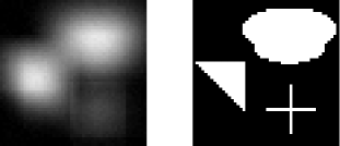
Figure 1: Observed image (left panel) and true image (right panel) in the 2D image deblurring example.

We model smoothness on $\boldsymbol{x}$ a priori by taking $\boldsymbol{L}=-\Delta+\delta\boldsymbol{I}$ in (3), where $-\Delta$ is the discrete Laplacian and $\delta$ is a small constant to ensure positive definiteness [37]. For the prior and noise precision parameters, we assign a vague Gamma prior, $\text{Gamma}(0.1,0.1)$, which approximates the scale invariant objective prior while maintaining conditional conjugacy. We compute the eigenvalues of the prior preconditioned Hessian matrix $\boldsymbol{H}$ via SVD to determine an appropriate cutoff. Figure 7 (discussed further below) indicates rapid decay within the first few eigenvalues, followed by a smoother decay, and another sharp decay. We use the first $k=500$ eigenvalues of the matrix to construct our low-rank approximation. We analyze below the effect of truncation level on the acceptance rate of the sampling algorithm. For comparison, we also compute a low-rank approximation using the Randomized SVD approach described in Subsection 3.4.

Convergence and UQ metrics

We implement a Metropolis-Hastings-within-Gibbs algorithm in which Step 1 of Algorithm 1 is substituted with our proposed low rank independence sampler (LRIS) presented in Section 3. Three different chains are run in parallel, with each chain initialized by drawing $\boldsymbol{x},\mu$, and $\sigma$ randomly from their prior distributions. Each chain is run for $N=50,000$ iterations with the first $25,000$ iterations discarded as a burn-in period. For comparison, the Gibbs sampler is implemented identically to the low-rank procedure with three independent chains run in parallel with widely dispersed initial values. All simulations are done in MATLAB running on OS X Yosemite (8GB RAM, Intel Core i5 2.66GHz processor).

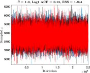
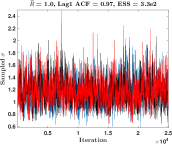
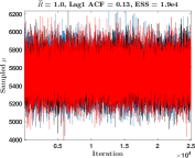
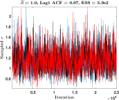
Figure 2: Trace plots of $\mu$ (left) and $\sigma$ (right) obtained from the MCMC output of both block Gibbs sampling (top row) and the LRIS-based algorithm (bottom row), where each of the three colors represents a different chain. The potential scale reduction factors ($\widehat{R}$) are displayed above each plot, along with the lag 1 autocorrelation coefficients and effective sample size (ESS) estimated from one chain each under both approaches.

Figures 2 and 3 display trace plots and autocorrelation functions, respectively, for the last $25,000$ iterations of the $\mu$ and $\sigma$ chains for both ordinary block Gibbs sampling and our proposed algorithm. As is known to occur with block Gibbs sampling in high-dimensional linear inverse problems [5], we observe near independence within the $\mu$ chains and strong autocorrelation in the $\sigma$ chains. Despite the high autocorrelation, we still are able to achieve approximate convergence and a sufficient effective sample size (ESS) from the $\sigma$ chains by running each chain long enough. By combining the three independent chains after approximate convergence, we effectively triple the ESS and thus the number of independent pieces of information available about the target posterior. Thinning the chains to, e.g., every $10$th, $50$th, or $100$th draw would dramatically reduce the autocorrelation of the chains. However, it was argued by Carlin and Louis [14] that such thinning is not necessary and does not improve estimates of quantities of interest. Figure 4 illustrates the approximate convergence of the ergodic averages $\widehat{\mu}_{(n)}=n^{-1}\sum_{t=1}^{n}\mu_{(t)}$ and $\widehat{\sigma}_{(n)}=n^{-1}\sum_{t=1}^{n}\sigma_{(t)},~{}n=1,\ldots,25000,$ despite the high autocorrelation of the $\sigma$ chain. The limiting values from both approaches closely agree.

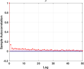
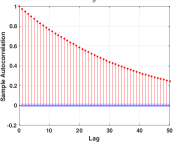
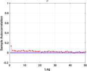
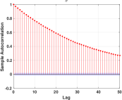
Figure 3: Estimated autocorrelation functions of $\mu$ (left) and $\sigma$ (right) obtained from one of the chains each under block Gibbs sampling (top row) and our proposed LRIS algorithm (bottom row).

While assessing convergence of high-dimensional parameters is more difficult than for scalar quantities, we can track realized values of the data-misfit part of the log-likelihood as a proxy for monitoring convergence. These realizations also should settle down as the chain approaches the target distribution. Figure 4 displays these plots for both algorithms along with the multivariate PSRFs. Again, we see consistency between ordinary block Gibbs and our own approach, as well as approximate convergence according to the rule of thumb that the PSRF should be less than or equal to approximately 1.1 [22].

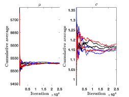
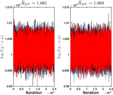
Figure 4: Cumulative averages of the $\mu$ chains (far left) and $\sigma$ chains (middle left) obtained from the MCMC output in the 2D deblurring example. The dotted lines represent the three chains from block Gibbs, the solid lines correspond to the LRIS algorithm output. Plot of the data-misfit part of the log-likelihood values calculated from the MCMC output of both block Gibbs sampling (middle right) and our low-rank independence sampling algorithm (far right), where each of the three colors corresponds to a different chain. The multivariate potential scale reduction factors are displayed above.

The advantage of using the LRIS approach is clear in Table 2, which displays the total wall time to complete the $50,000$ MCMC iterations for both block Gibbs and our proposed low-rank sampling approach. Table 2 also displays the cost per effective sample (CES) for one of the $\sigma$ chains obtained under both algorithms as well as the Randomized SVD approach. CES is a measure of the average computational effort required between effectively independent draws. The LRIS approach yields a 76% reduction in computation time compared to the standard block Gibbs sampler, along with an approximate 80% reduction in computational effort between independent draws of $\sigma$. The average acceptance rate over the three chains using our low-rank proposals is 98%, for both “exact" and Randomized SVD. The acceptance rate versus rank is discussed further below.

Algorithm	Wall Time (s)	CES for $\sigma$
Block Gibbs	27907	84.30
LRIS	5134	13.20
LRIS (Randomized SVD)	5307	13.86

Table 2: Total wall time to complete $50,000$ MCMC iterations under block Gibbs sampling and the LRIS approach for the 2D deblurring example, along with the estimated cost per effective sample (CES) for one of the $\sigma$ chains in each case.

We attain this dramatic reduction in computational effort without sacrificing the quality of posterior inferences, as evident in Figure 5. This Figure displays the approximate posterior means of $\boldsymbol{x}$ from both block Gibbs and our low-rank approach. The estimators we obtain with Randomized SVD are similar and hence omitted. We show also the $(\mu,\sigma)$ scatterplots and approximate marginal densities obtained from both algorithms in Figure 6, again showing agreement. The strong Bayesian learning that occurred about these parameters is evident in Supplementary Figure S11. Table 3 gives the relative errors to quantify the quality of the reconstructions. We observe nearly identical solutions under both MCMC approaches, both graphically and quantitatively.

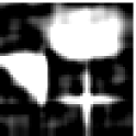
Figure 5: Approximate posterior mean images obtained from block Gibbs sampling (left) and the proposed low-rank sampling algorithm (right) for the 2D deblurring example.

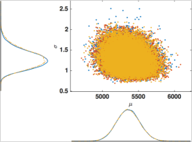
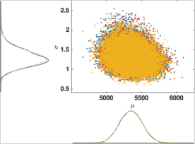
Figure 6: Scatter plots of the $(\mu,\sigma)$ realizations obtained from block Gibbs (left panel) and the low-rank approach (right panel) for the 2D deblurring example, where the three different colors correspond to different chains. The smoothed marginal posterior densities are displayed in the margins of the plots.

Estimator	RE
Posterior Mean (Block Gibbs)	0.4453
Posterior Mean (LRIS)	0.4455

Table 3: Relative error (RE) of the estimates for the 2D image deblurring example.

Acceptance rate versus rank

To explore the effect of the retained number of eigenvalues on the acceptance rate for our algorithm, we estimate the predicted and empirical acceptance rates of sampling from the proposal distribution, over a range of truncation levels, at a given state of the chain. We fix the state by initializing $(\boldsymbol{x},\mu,\sigma)$ as the last sample from one of the chains obtained from the LRIS. At each truncation level $k$, we compute the expected value of the acceptance ratio using Theorem 1. We draw $2,000$ samples from the proposal distribution and compute the acceptance ratio of each using Proposition 2. From these we estimate the empirical failure rates to compare with their expected values as the truncation level increases. Figure 7 displays the results. The close agreement between the predicted and empirical acceptance rates support the theoretical results in Section 3.

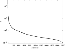
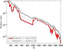
Figure 7: (left) Eigenvalues of $\boldsymbol{H}$ in the 2D image deblurring example. (right) Predicted and empirical failure rates for different truncation levels $K$. The empirically determined upper $0.975$ quantile is given by the dashed line; the lower quantile often attained zero values, so it is not displayed.

4.2 CT Image Reconstruction

Computed x-ray tomography (CT) is a common medical imaging modality in which x-rays are passed through a body from a source to a sensor along parallel lines indexed by an angle $\omega$ and offset $y$ with respect to a fixed coordinate system and origin. The intensities of the rays are attenuated according to an unknown absorption function as they pass through tissue. The attenuated intensity $I$ is recorded while the lines are rotated around the origin so that $I(S)=I(0)\exp\{-\int_{0}^{S}\alpha(x(s))\,\mathrm{d}s\}$, where $s=0$ is the source of the x-ray, $s=S$ is the receiver location, $x(\cdot)$ indicates the line position, and $\alpha$ is the absorption function. The observed data are a transformation of the intensities, yielding the Radon transform model for CT [37, 4], $z(\omega,y)=\int_{L(\omega,y)}\alpha(x(s))\,\mathrm{d}s$, where $L(\omega,y)$ is the line along which the x-ray passes through the body. The inverse problem is to reconstruct the absorption function, which provides an image of the scanned body. Discretization of the integral yields the model in (1). This is typically an underdetermined system with infinitely many solutions, resulting in an ill-posed inverse problem.

Our target image is the Shepp-Logan phantom [62]. The forward model is implemented in MATLAB on the same computer as in Subsection 4.1 with code available online [3]. The data are simulated by adding Gaussian noise with variance $0.01^{2}\|\boldsymbol{Ax}\|_{\infty}^{2}$. The target $\alpha$ is discretized to a relatively fine grid of size $128\times 128$ so that $\dim(\boldsymbol{x})=16,384$. We suppose that the data are observed over lines and angles such that $\dim(\boldsymbol{b})=5000$. Thus, $\text{rank}(\boldsymbol{A})=5000\ll\dim(\boldsymbol{x})$, guiding our choice of eigenvalue truncation in the low-rank approximation to $\boldsymbol{H}$. An approximate eigendecomposition of the prior preconditioned Hessian is computed using Randomized SVD with $\ell=5000$, as discussed in Section 3, since computing the “exact" SVD is considerably more expensive. As in Subsection 4.1, we take $\boldsymbol{L}=-\Delta+\delta\boldsymbol{I}$.

For the nuisance parameters, we use a weakly informative prior [21], namely the proper Jeffreys prior proposed by Scott and Berger [60]. For convenience, we parameterize the model in terms of variance components instead of precisions, $\tau^{2}:=\sigma^{-1}$ and $\kappa^{2}:=\mu^{-1}$. Then the proper Jeffreys prior on $(\kappa^{2},\tau^{2})$ is

$$\begin{aligned} \pi_{SB}(\kappa^{2},\tau^{2})&=(\kappa^{2}+\tau^{2})^{-2}\\ &=(\kappa^{2})^{-1}(1+\tau^{2}/\kappa^{2})^{-2}\times(\kappa^{2})^{-1}\\ &\equiv\pi(\tau^{2}\mid\kappa^{2})\pi(\kappa^{2}),\end{aligned}$$ (16)

so that the scale invariant prior is used for $\kappa^{2}$ while scaling $\tau^{2}$ by the data level variance, as advocated by Jeffreys [33]. The implementation of this prior as a modification to Algorithm 1, presented in Appendix B, is similar to the approach of [11]. Section B of the Supplementary Material contains further discussion of prior specification for the nuisance parameters.

We simulate three Markov chains using our proposed LRIS approach for $40,000$ iterations (average acceptance rate $\sim 100\%$). Each chain is initialized with values drawn randomly from the prior. We thin the chains by retaining every $50\text{th}$ draw to reduce the autocorrelation, making it easier to diagnose convergence. We discard the first $400$ draws of the thinned chains as a burn-in period. Trace plots and autocorrelation plots are used to verify approximate convergence of the chains. Relevant diagnostic plots are displayed in Supplementary Figures S12, S13, and S14. The total computation time for our sampling approach is $197,517$ seconds, or about $55$ hours. This is noteworthy since the algorithm repeatedly updates a large, nontrivial covariance matrix and samples an approximately sixteen-thousand dimensional Gaussian distribution 40,000 times. An ordinary block Gibbs sampler is simply not feasible for this problem.

We compare the results with samples obtained using the conjugate Gamma model with the same vague priors on $\mu$ and $\sigma$ as in Subsection 4.1. Convergence diagnostics are displayed in Supplementary Figures S15 and S16. Figure 8 compares the approximate joint distributions for the precision parameters $(\mu,\sigma)$ under the conjugate model to the distribution based on the proper Jeffreys model, after back-transforming $\kappa^{2}$ and $\tau^{2}$. Here we see the effect of prior selection in that both $\mu$ and $\sigma$ tend to concentrate around different values, with much greater uncertainty in $\mu$ in the proper Jeffreys case. The differences between the two marginal posteriors of $(\mu,\sigma)$ affect the quality of the reconstructed images, displayed in Figure 9 and quantified in Table 4. This echoes Gelman’s observation [21] that even a supposedly noninformative prior on the hyper-precision can have a disproportionate influence on the results. In this case, using a weakly informative prior for $\sigma$ that depends on $\mu$ results in a higher quality reconstruction.

Scale parameter prior	RE
Proper Jeffreys	0.3270
Conjugate Gamma	0.4229

Table 4: Relative error (RE) of the estimates for the CT image reconstruction example.

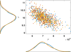
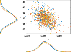
Figure 8: Estimated joint densities for the precision parameters using the proper Jeffreys prior (left) and the conjugate Gamma priors (right).

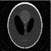
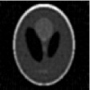
Figure 9: Posterior mean estimators of the true image in the CT image reconstruction example, using the proper Jeffreys prior (left) and the conjugate Gamma priors (right).

These simulations show that by exploiting the low-rank structure of the preconditioned Hessian of the forward model, we are able to substantially reduce the computational burden compared to block Gibbs sampling. Even when the forward model is of full row rank, the results illustrate the potential for efficiency gains using our proposed LRIS approach, provided the system is underdetermined. Our approach using either proper Jeffreys or conjugate priors is much more feasible than a block Gibbs sampler, for which the computational demands can be prohibitively expensive. A comparison of the conventional conjugate Gamma priors to a weakly informative prior suggests that even a “noninformative" prior may exert considerable influence on the results, despite strong Bayesian learning in the posterior.

In the Supplementary Material, we further consider the challenging problem of nuclear magnetic resonance (NMR) relaxometry. There, we demonstrate that our approach still produces within reasonable computation time a solution that is comparable to those obtained from deterministic iterative procedures such as conjugate gradient least squares. This is achieved with randomized SVD and without explicitly forming the forward operator $\boldsymbol{A}$ in the LRIS algorithm.

5 Discussion

When approximating the posterior distribution via Markov chain Monte Carlo in the Bayesian Gaussian linear inverse problem, the bottleneck is in repeatedly sampling high-dimensional Gaussian random variables. Sampling from the joint posterior with standard MCMC is challenging due to the high dimensionality of the estimand, since drawing from the full conditional involves expensive operations with the covariance matrix.

In this work we propose a computationally efficient sampling algorithm which is well suited for a fully Bayesian approach in which the noise precision and the prior precision parameters are unknown and assigned prior distributions. Our proposed low rank independence sampler uses a proposal distribution constructed via low-rank approximation to the preconditioned Hessian. We show that the acceptance rate is high when the magnitudes of the discarded eigenvalues of the Hessian are small, a feature of severely ill-posed problems. When it is not obvious how to determine an appropriate truncation of rank due to the dependence of the known acceptance rates on other parameters in the model, we discuss how to adaptively determine the truncation level as part of the MCMC algorithm to find the minimal rank with high acceptance rates. We demonstrate both theoretically and empirically that the quality of the approximation is directly related to the acceptance rate of the sampler, as intuition would suggest. We illustrate our approach on several examples, demonstrating convergence as function of rank, as well as computational improvements to accessing the full posterior distribution.

A known issue with block Gibbs sampling in Bayesian inverse problems is the deterioration of the chains due to correlation between the hyperparameters and the estimand $\boldsymbol{x}$ as the dimension of the problem increases [5]. Several approaches have been proposed to ameliorate this by breaking the dependence between the hyperparameters and $\boldsymbol{x}$ in the algorithm. These include the one-block algorithm [54], partially collapsed samplers [67, 7], noncentered parameterization (NCP) [45, 46], and marginal then conditional (MTC) sampling [17]. Noncentered parameterization is easily incorporated into our proposed approach without sacrificing gains in efficiency. (See the Supplementary Material for discussion of NCP and illustration of combining it with our low-rank sampler.) One-block sampling and MTC, on the other hand, require expressions for marginal densities that no longer hold when substituting the true full conditional of $\boldsymbol{x}$ with an approximation, as well as approximation of determinants of large covariance matrices to which the results in this work are not directly applicable. Combining our proposed low-rank sampling approach with these algorithms is the subject of ongoing research, to appear in future work.

6 Acknowledgements

DAB is partially supported by Grants CMMI-1563435 and EEC-1744497 from the National Science Foundation (NSF). This material is based upon work partially supported by the NSF under Grant DMS-1127914 to the Statistical and Applied Mathematical Sciences Institute (SAMSI). The authors thank the Editors, an Associate Editor, and anonymous referees for comments and suggestions that improved this manuscript. The authors also would like to thank Duy Thai, Vered Madar, Johnathan Bardsley, and Ray Falk for useful conversations. Much of this work was done while the first author was a Visiting Research Fellow at SAMSI.

Appendix A Proofs

Proof of Proposition 2: The difference between the true and the approximate covariance matrices can be expressed as

$$\boldsymbol{\Gamma}_{\text{cond}}^{-1}-\widehat{\boldsymbol{\Gamma}}_{\text{cond}}^{-1}= \>\mu\boldsymbol{A}^{\top}\boldsymbol{A}+\sigma\boldsymbol{L}^{\top}\boldsymbol{L}-\left(\mu\boldsymbol{L}^{\top}\boldsymbol{V}_{k}\boldsymbol{\Lambda}_{k}\boldsymbol{V}_{k}^{\top}\boldsymbol{L}+\sigma\boldsymbol{L}^{\top}\boldsymbol{L}\right),$$

$$= \>\mu\boldsymbol{L}^{\top}\left(\boldsymbol{L}^{-\top}\boldsymbol{A}^{\top}\boldsymbol{A}\boldsymbol{L}^{-1}-\boldsymbol{V}_{k}\boldsymbol{\Lambda}_{k}\boldsymbol{V}_{k}^{\top}\right)\boldsymbol{L},$$

$$= \>\mu\boldsymbol{L}^{\top}\left(\sum_{j=k+1}^{n}\lambda_{j}\boldsymbol{v}_{j}\boldsymbol{v}_{j}^{\top}\right)\boldsymbol{L},$$

giving that $\log w(\boldsymbol{x})=-\frac{\mu}{2}\sum_{j=k+1}^{n}\lambda_{j}\left(\boldsymbol{v}_{j}^{\top}\boldsymbol{Lx}\right)^{2}\leq 0,$ and hence the acceptance ratio is given by (11). $\square$

Lemma 1.

Suppose $\boldsymbol{M}$ is symmetric positive definite. Then,

$$\int_{\mathbb{R}^{n}}\exp\left(-\frac{1}{2}\boldsymbol{z}^{T}\boldsymbol{Mz}+\boldsymbol{J}^{\top}\boldsymbol{z}\right)d\boldsymbol{z}\>=\>\frac{(2\pi)^{n/2}}{\det(\boldsymbol{M})^{1/2}}\exp\left(\frac{1}{2}\boldsymbol{J}^{\top}\boldsymbol{M}^{-1}\boldsymbol{J}\right).$$

Proof.

See [59, Lemma B.1.1]. ∎

Lemma 2.

The moments of the acceptance ratio are

$$\mathbb{E}_{\boldsymbol{z}|\boldsymbol{x}}[\eta^{m}(\boldsymbol{z},\boldsymbol{x})]\>=\>\frac{1}{N_{m}w^{m}(\boldsymbol{x})}\,,$$

where $N_{m}$ is defined in (12).

Proof.

The proof proceeds in four steps.

1. Simplifying $\mathbb{E}_{\boldsymbol{z}|\boldsymbol{x}}[w^{m}(\boldsymbol{z})]$. We focus on $\mathbb{E}_{\boldsymbol{z}|\boldsymbol{x}}[w^{m}(\boldsymbol{z})]$. By definition, this is

$$\int_{\mathbb{R}^{n}}w^{m}(\boldsymbol{z})g(\boldsymbol{z})d\boldsymbol{z}=\frac{\exp\left(-\frac{1}{2}(\hat{\boldsymbol{x}}_{\text{cond}})^{\top}\widehat{\boldsymbol{\Gamma}}_{\text{cond}}^{-1}\hat{\boldsymbol{x}}_{\text{cond}}\right)}{(2\pi)^{n/2}\det(\widehat{\boldsymbol{\Gamma}}_{\text{cond}})^{1/2}}\int\exp\left(-\frac{1}{2}\boldsymbol{z}^{T}\boldsymbol{Mz}+\boldsymbol{J}^{\top}\boldsymbol{z}\right)d\boldsymbol{z},$$

where, by using $\hat{\boldsymbol{x}}_{\text{cond}}=\mu\widehat{\boldsymbol{\Gamma}}_{\text{cond}}\boldsymbol{A}^{\top}\boldsymbol{b}$, we get,

$$\boldsymbol{M}=m(\boldsymbol{\Gamma}_{\text{cond}}^{-1}-\widehat{\boldsymbol{\Gamma}}_{\text{cond}}^{-1})+\widehat{\boldsymbol{\Gamma}}_{\text{cond}}^{-1},~{}~{}\text{ and }~{}~{}\boldsymbol{J}=\widehat{\boldsymbol{\Gamma}}_{\text{cond}}^{-1}\hat{\boldsymbol{x}}_{\text{cond}}=\mu\boldsymbol{A}^{\top}\boldsymbol{b}.$$

Applying Lemma 1 and rearranging, we have

$$\mathbb{E}_{\boldsymbol{z}|\boldsymbol{x}}[w^{m}(\boldsymbol{z})]=\frac{\exp\left(\frac{\mu^{2}}{2}(\boldsymbol{A}^{\top}\boldsymbol{b})^{\top}(\boldsymbol{M}^{-1}-\widehat{\boldsymbol{\Gamma}}_{\text{cond}})\boldsymbol{A}^{\top}\boldsymbol{b}\right)}{\det(\boldsymbol{M})^{1/2}\det(\widehat{\boldsymbol{\Gamma}}_{\text{cond}})^{1/2}}.$$ (17)

We focus on the numerator and denominator of (17) separately.

2. Denominator of (17). Note that

$$\boldsymbol{M}=m(\boldsymbol{\Gamma}_{\text{cond}}^{-1}-\widehat{\boldsymbol{\Gamma}}_{\text{cond}}^{-1})+\widehat{\boldsymbol{\Gamma}}_{\text{cond}}^{-1}=m\boldsymbol{\Gamma}_{\text{cond}}^{-1}+(1-m)\widehat{\boldsymbol{\Gamma}}_{\text{cond}}^{-1}$$

and furthermore,

$$\boldsymbol{M}=\boldsymbol{L}^{\top}\left(\mu\sum_{j=1}^{k}\lambda_{j}\boldsymbol{v}_{j}\boldsymbol{v}_{j}^{\top}+m\mu\sum_{j=k+1}^{n}\lambda_{j}\boldsymbol{v}_{j}\boldsymbol{v}_{j}^{\top}+\sigma\boldsymbol{I}\right)\boldsymbol{L}.$$

Using the properties of determinants, it can be shown that

$$\det(\boldsymbol{M})=\sigma^{n}\det(\boldsymbol{L})^{2}\prod_{j=1}^{k}\left(1+\frac{\mu}{\sigma}\lambda_{j}\right)\prod_{j=k+1}^{n}\left(1+\frac{m\mu}{\sigma}\lambda_{j}\right).$$

Similarly,

$$\det(\widehat{\boldsymbol{\Gamma}}_{\text{cond}}^{-1})=\sigma^{n}\det(\boldsymbol{L})^{2}\prod_{j=1}^{k}\left(1+\frac{\mu}{\sigma}\lambda_{j}\right).$$

Combining these results, the denominator of (17) becomes

$$\det(\boldsymbol{M})^{1/2}\det(\widehat{\boldsymbol{\Gamma}}_{\text{cond}})^{1/2}=\sqrt{\frac{\det(\boldsymbol{M})}{\det(\widehat{\boldsymbol{\Gamma}}_{\text{cond}})}}=\prod_{j>k}\left(1+\frac{m\mu}{\sigma}\lambda_{j}\right)^{1/2}.$$

3. Numerator of (17). Consider $\boldsymbol{M}^{-1}-\widehat{\boldsymbol{\Gamma}}_{\text{cond}}$. By the Woodbury matrix identity,

$$\boldsymbol{M}^{-1}-\widehat{\boldsymbol{\Gamma}}_{\text{cond}}= \left(m\boldsymbol{\Gamma}_{\text{cond}}^{-1}+(1-m)\widehat{\boldsymbol{\Gamma}}_{\text{cond}}^{-1}\right)^{-1}-\widehat{\boldsymbol{\Gamma}}_{\text{cond}}$$

$$= \frac{1}{\sigma}\boldsymbol{L}^{-1}\left(\boldsymbol{I}-\sum_{j=1}^{k}\frac{\mu\lambda_{j}}{\mu\lambda_{j}+\sigma}\boldsymbol{v}_{j}\boldsymbol{v}_{j}^{\top}-\sum_{j=k+1}^{n}\frac{m\mu\lambda_{j}}{m\mu\lambda_{j}+\sigma}\boldsymbol{v}_{j}\boldsymbol{v}_{j}^{\top}\right)\boldsymbol{L}^{-\top}$$

$$\qquad-\frac{1}{\sigma}\left(\boldsymbol{I}-\sum_{j=1}^{k}\frac{\mu\lambda_{j}}{\mu\lambda_{j}+\sigma}\boldsymbol{v}_{j}\boldsymbol{v}_{j}^{\top}\right)\boldsymbol{L}^{-\top}$$

$$= -\frac{1}{\sigma}\sum_{j=k+1}^{n}\frac{m\mu\lambda_{j}}{m\mu\lambda_{j}+\sigma}\boldsymbol{L}^{-1}\boldsymbol{v}_{j}\boldsymbol{v}_{j}^{\top}\boldsymbol{L}^{-\top}.$$

The numerator is therefore,

$$\exp\left(\frac{\mu^{2}}{2}(\boldsymbol{A}^{\top}\boldsymbol{b})^{\top}(\boldsymbol{M}^{-1}-\widehat{\boldsymbol{\Gamma}}_{\text{cond}})\boldsymbol{A}^{\top}\boldsymbol{b}\right)=\exp\left(-\frac{\mu^{2}}{2\sigma}\sum_{j=k+1}^{n}\frac{m\mu\lambda_{j}}{m\mu\lambda_{j}+\sigma}(\boldsymbol{b}^{\top}\boldsymbol{A}\boldsymbol{L}^{-1}\boldsymbol{v}_{j})^{2}\right).$$

4. Combining intermediate results. Plugging the results of Steps 2 and 3 into (17) gives us $\mathbb{E}_{\boldsymbol{z}|\boldsymbol{x}}[w^{m}(\boldsymbol{z})]=\frac{1}{N_{m}}$, where $N_{m}$ is defined in (12). The proof readily follows because $\mathbb{E}_{\boldsymbol{z}|\boldsymbol{x}}[\eta^{m}(\boldsymbol{z},\boldsymbol{x})]=\mathbb{E}_{\boldsymbol{z}|\boldsymbol{x}}[w^{m}(\boldsymbol{z})]/w^{m}(\boldsymbol{x})$. ∎

Proof of Theorem 1: From Lemma 2, we have $\mathbb{E}_{\boldsymbol{z}|\boldsymbol{x}}[\eta^{m}(\boldsymbol{z},\boldsymbol{x})]\>=\>\frac{1}{N_{m}w^{m}(\boldsymbol{x})}$. The first result follows immediately by plugging in $m=1$. For the second result, we use the fact that for a random variable $X$ with $\mathbb{E}(X^{2})<\infty$, $\mathbb{V}[X]=\mathbb{E}[(X-\mathbb{E}[X])^{2}]=\mathbb{E}[X^{2}]-(\mathbb{E}[X])^{2}$. The result follows from (13) and applying Lemma 2 with $m=2$. $\square$

Proof of Proposition 3: Using $h$ as defined in (10) and the definition of the proposal density $g$,

$$\frac{h(\boldsymbol{x})}{g(\boldsymbol{x})}=\sqrt{\frac{\det(\widehat{\boldsymbol{\Gamma}}_{\text{cond}})}{\det(\boldsymbol{\Gamma}_{\text{cond}})}}\ w(\boldsymbol{x})\exp\left(-\frac{\mu^{2}}{2}\boldsymbol{b^{\top}A}(\boldsymbol{\Gamma}_{\text{cond}}-\widehat{\boldsymbol{\Gamma}}_{\text{cond}})\boldsymbol{A^{\top}b}\right).$$

From the proof of Lemma 2, $\boldsymbol{M}^{-1}=\boldsymbol{\Gamma}_{\text{cond}}$ when $m=1$. Comparing terms with (17) this gives us $h(\boldsymbol{x})=N_{1}g(\boldsymbol{x})w(\boldsymbol{x})$, where $N_{1}$ is defined in (12). From the proof of Proposition 2, $\log w(\boldsymbol{x})\leq 0$, and therefore $w(\boldsymbol{x})\leq 1$. The desired result follows. Note that the bound is tight because $w(\boldsymbol{0})=1$. $\square$

Proof of Theorem 2: It is easy to show that $w(\boldsymbol{x})\leq 1$, therefore, $\eta(\boldsymbol{z},\boldsymbol{x})\geq w(\boldsymbol{z})$. From Proposition 1, we need to consider the quadratic form

$$\frac{1}{2}\boldsymbol{z}^{\top}(\boldsymbol{\Gamma}_{\text{cond}}^{-1}-\widehat{\boldsymbol{\Gamma}}_{\text{cond}}^{-1})\boldsymbol{z}=\frac{\mu}{2}\boldsymbol{z}^{\top}\boldsymbol{L}^{\top}(\boldsymbol{H}-\widehat{\boldsymbol{H}})\boldsymbol{Lz},$$

where $\widehat{\boldsymbol{H}}$ is the low-rank approximation, see (15). This follows from $\widehat{\boldsymbol{\Gamma}}_{\text{cond}}^{-1}=(\mu\boldsymbol{L}^{\top}\widehat{\boldsymbol{H}}\boldsymbol{L}+\sigma\boldsymbol{L}^{\top}\boldsymbol{L})$. Using the Cauchy-Schwartz inequality, we can bound (in the spectral norm)

$$\boldsymbol{z}^{\top}\boldsymbol{L}^{\top}(\boldsymbol{H}-\widehat{\boldsymbol{H}})\boldsymbol{Lz}\leq\|\boldsymbol{Lz}\|^{2}_{2}\|\boldsymbol{H}-\widehat{\boldsymbol{H}}\|_{2}.$$

Arguing as in [26, Section 5.3], we have $\|\boldsymbol{H}-\widehat{\boldsymbol{H}}\|_{2}\leq 2\|\boldsymbol{H}-\boldsymbol{QQ}^{\top}\boldsymbol{H}\|_{2}$. Applying [26, Theorem 10.6] we have

$$\mathbb{E}_{\boldsymbol{\Omega}}\,\|\boldsymbol{H}-\widehat{\boldsymbol{H}}\|_{2}\>\leq\>2\left[\alpha\lambda_{k+1}+\beta\left(\sum_{j=k+1}^{n}\lambda_{j}^{2}\right)^{1/2}\right],$$ (18)

with constants $\alpha$ and $\beta$ given in the statement of the result. Applying Jensen’s inequality

$$\mathbb{E}_{\boldsymbol{\Omega}}\,[\eta(\boldsymbol{z},\boldsymbol{x})]\geq\exp\left(-\mu\|\boldsymbol{Lz}\|^{2}\mathbb{E}_{\boldsymbol{\Omega}}\,\|\boldsymbol{H}-\widehat{\boldsymbol{H}}\|_{2}\right).$$

Plug in (18) into the above equation to complete the proof. $\square$

Appendix B Implementing the Proper Jeffreys Prior

Here we briefly discuss an implementation of the LRIS algorithm when the Scott-Berger prior (16) is used instead of the independent conjugate Gamma priors.

In this case, the model (16) becomes

$$\begin{aligned} \boldsymbol{y}\mid\boldsymbol{x},\kappa^{2}&\sim N(\boldsymbol{Ax},\kappa^{2}\boldsymbol{I})\\ \boldsymbol{x}\mid\tau^{2}&\sim N(\boldsymbol{0},\tau^{2}\boldsymbol{\Gamma})\\ \pi(\tau^{2}\mid\kappa^{2})&=\kappa^{-2}(1+\tau^{2}/\kappa^{2})^{-2}\\ \pi(\kappa^{2})&=\kappa^{-2}.\end{aligned}$$ (19)

To obtain the full conditional densities necessary for Gibbs sampling, it is convenient to reparameterize the model with $\upsilon=\tau^{2}/\kappa^{2}$. After the change of variables, the joint posterior (5) becomes

$$\begin{aligned} \pi(\boldsymbol{x},\kappa^{2},\upsilon\mid\boldsymbol{b})&\propto(\kappa^{2})^{-\frac{m+n}{2}-1}\upsilon^{-n/2}(1+\upsilon)^{-2}\\ &\quad\times\exp\left(-\frac{1}{2\kappa^{2}}\left[\|\boldsymbol{Ax}-\boldsymbol{b}\|^{2}_{2}+\frac{1}{\upsilon}\|\boldsymbol{Lx}\|^{2}_{2}\right]\right).\end{aligned}$$ (20)

The full conditional on $\boldsymbol{x}$ is a standard result for the Normal-Normal model (4); i.e.

$$\boldsymbol{x}\mid\kappa^{2},\upsilon,\boldsymbol{b}\sim\mathcal{N}(\boldsymbol{x}_{\text{cond}},\boldsymbol{\Gamma}_{\text{cond}}),$$

where $\boldsymbol{\Gamma}_{\text{cond}}=\kappa^{2}\left(\boldsymbol{A}^{\top}\boldsymbol{A}+\upsilon^{-1}\boldsymbol{\Gamma}_{\text{pr}}^{-1}\right)^{-1}$ and $\boldsymbol{x}_{\text{cond}}=\left(\boldsymbol{A}^{\top}\boldsymbol{A}+\upsilon^{-1}\boldsymbol{\Gamma}_{\text{pr}}^{-1}\right)^{-1}\boldsymbol{A}^{\top}\boldsymbol{b}$. We can sample from this density using our proposed low-rank approximation approach. (See Section 3.) The full conditional on $\kappa^{2}$ is

$$\kappa^{2}\mid\boldsymbol{x},\upsilon,\boldsymbol{y}\sim\text{InvGamma}\left(\frac{m+n}{2},\frac{1}{2}\|\boldsymbol{Ax}-\boldsymbol{b}\|^{2}_{2}+\frac{1}{2\upsilon}\|\boldsymbol{Lx}\|^{2}_{2}\right).$$

To draw from this density, draw $W\sim\text{Gamma}\left(\frac{m+n}{2},\frac{1}{2}\|\boldsymbol{Ax}-\boldsymbol{b}\|^{2}_{2}+\frac{1}{2\upsilon}\|\boldsymbol{Lx}\|^{2}_{2}\right)$ and set $\kappa^{2}=1/W$. The full conditional on $\upsilon$ is

$$\pi(\upsilon\mid\boldsymbol{x},\kappa^{2},\boldsymbol{b}) \propto\upsilon^{-(n/2+1)-1}\exp\left[-\frac{1}{2\kappa^{2}\upsilon}\|\boldsymbol{Lx}\|^{2}_{2}\right]\left(\frac{\upsilon}{1+\upsilon}\right)^{2}$$ (21)

$$\equiv h(\upsilon)\left(\frac{\upsilon}{1+\upsilon}\right)^{2},$$ (22)

where $h(\upsilon)$ is the density of an $\text{InvGamma}((n+2)/2,\|\boldsymbol{Lx}\|^{2}_{2}/(2\kappa^{2}))$ distribution. Thus we can use an independence Metropolis-Hastings algorithm with candidate distribution

$$\text{InvGamma}((n+2)/2,\|\boldsymbol{Lx}\|^{2}_{2}/(2\kappa^{2})).$$

This Supplementary Material contains additional material referenced in the manuscript that could aid the reader, but is not essential. We empirically demonstrate mixing behavior and efficiency of an LRIS-based Metropolis-Hastings-within-Gibbs sampler as a function of rank of the approximation, elaborate on possibilities for prior modeling of the precision (variance) components in the hierarchical model for the Bayesian inverse problem, and discuss the use of noncentered parameterization in our proposed LRIS algorithm, supported by application to the 2D deblurring example. We further demonstrate computational feasibility afforded by our proposed approach by considering MCMC/LRIS-based reconstruction of a distribution of relaxation times in nuclear magnetic resonance (NMR) relaxometry. Supplementary Figures are at the end.

Appendix A Effect of the Proposal Rank on Chain Mixing

To study how the quality of the low-rank approximation affects the mixing of an MCMC algorithm, we consider the image reconstruction problem originally appearing in [61]. This is a one-dimensional image restoration problem in which the blurred image can be expressed as a Fredholm integral equation of the first kind, $g(s)=\int_{-\pi/2}^{\pi/2}K(s,t)f(t)\,\mathrm{d}t,$ where $K(s,t)=(\cos(s)+\cos(t))^{2}\left(\sin(u)/u\right)^{2}$ with $u=\pi(\sin(s)+\sin(t))$, and $f$ is the true one-dimensional image given by $f(t)=2\exp(-6(t-0.8)^{2})+\exp(-2(t+0.5)^{2})$. The problem is to reconstruct $f$ given $g$ and $K$. Using the implementation in the Matlab package Regularization Tools [27], we discretize the integral via quadrature over $n=512$ points and corrupt the observations with one percent noise. The resulting model is $\boldsymbol{b}=\boldsymbol{Ax}+\boldsymbol{\epsilon},~{}\boldsymbol{\epsilon}\sim\mathcal{N}(\boldsymbol{0},\boldsymbol{\Gamma}),$ where $\boldsymbol{b}$ is the observed data, $\boldsymbol{A}\in\mathbb{R}^{n\times n}$ is the discretized forward model, $\boldsymbol{x}$ is the discretized solution, and $\boldsymbol{\Gamma}=0.01^{2}\|\boldsymbol{b}\|^{2}\boldsymbol{I}$. The observed data $\boldsymbol{b}$ and solution $f$ are displayed in Figure S1.

In the hierarchical Bayesian model, we use a zero mean Gaussian process (GP) prior [59, 50], $f(\cdot)\sim\mathcal{GP}(0,\sigma^{-1}R(\cdot,\cdot))$. We take the correlation function to be in the power exponential family, $R(t_{i},t_{j})=\exp\left(-|t_{i}-t_{j}|/l\right)$, with correlation length parameter $l=\pi/2$. We use vague Gamma priors about the noise precision $\mu$ and prior precision $\sigma$ with $a_{\mu}=b_{\mu}=a_{\sigma}=b_{\sigma}=0.1$. We remark that for this example, the forward model is fast-running so that our computationally-cheap LRIS is actually not necessary. However, the fast-running model makes it feasible to run a large number of replicate MCMC chains in a reasonable amount of time, thus allowing us to empirically assess the mixing behavior of our proposed approach as a function of rank of the proposal distribution.

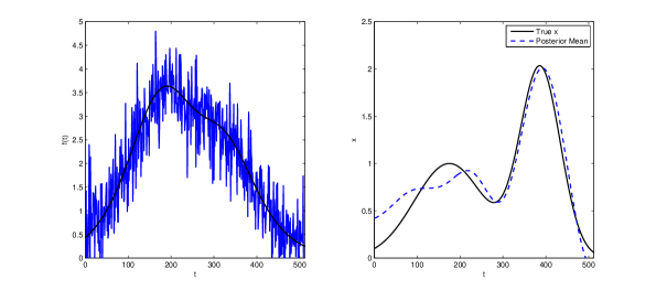
Figure S1: Observed data (left panel) and true solution (right panel) for the one-dimensional image restoration example. The solid black line in the left panel represents the noise-free observations $\boldsymbol{Ax}$. The dashed blue line is the true posterior mean (approximated from a very long block Gibbs Markov chain).

Similar to the analysis in [34], we consider two empirical measures to assess the mixing behavior of the Markov chains as a function of rank of the approximation in the LRIS algorithm. To assess the statistical efficiency of using the mean of the MCMC output to estimate $\mathbb{E}(\boldsymbol{x}\mid\boldsymbol{b})$, we use the mean squared error $MSE(\overline{\boldsymbol{x}}_{n}):=\mathbb{E}[(\overline{\boldsymbol{x}}_{n}-\mathbb{E}(\boldsymbol{x}\mid\boldsymbol{b}))^{2}]$, where $\overline{\boldsymbol{x}}_{n}$ is the sample mean of a chain of length $n$, $\boldsymbol{x}_{(1)},\ldots,\boldsymbol{x}_{(n)}$, obtained from an MCMC run. To approximate the MSE, we find the sample mean, $\overline{\boldsymbol{x}}^{\ast}$, from a very long run of an ordinary block Gibbs sampler and treat this as the true posterior mean $\mathbb{E}(\boldsymbol{x}\mid\boldsymbol{b})$. We run an additional $m$ independent Markov chains using LRIS-based Metropolis-Hastings-within-Gibbs, each of length $n$, whence we can approximate $MSE(\overline{\boldsymbol{x}}_{n})$ with $\widehat{MSE}(\overline{\boldsymbol{x}}_{n})=m^{-1}\sum_{i=1}^{m}(\overline{\boldsymbol{x}}_{n}^{(i)}-\overline{\boldsymbol{x}}^{\ast})^{2}$, where $\overline{\boldsymbol{x}}_{n}^{(i)}$ is the sample mean obtained from the $i^{\text{th}}$ chain. The second measure we consider is the expected squared Euclidean jump distance, defined as $ESEJD=\mathbb{E}(\|\boldsymbol{x}_{(t+1)}-\boldsymbol{x}_{(t)}\|_{2}^{2})$. This quantity is indicative of how well a Markov chain is exploring the marginal posterior distribution of the estimand $\boldsymbol{x}$. To approximate this expected value, we again run $m$ independent chains, each of length $n$. For each chain with rank $k$, we find the mean squared Euclidean jump distance $MSEJD_{k}:=(n-1)^{-1}\sum_{t=1}^{n-1}\|\boldsymbol{x}_{(t+1)}-\boldsymbol{x}_{(t)}\|_{2}^{2}$. Then we obtain an estimate of ESEJD with $\widehat{ESEJD}_{k}=m^{-1}\sum_{i=1}^{m}MSEJD_{k}^{(i)}$, where $MSEJD_{k}^{(i)}$ is mean squared Euclidean jump distance from the $i^{\text{th}}$ chain.

The left panel of Figure S2 displays the first ten eigenvalues of the prior-preconditioned Hessian for the one-dimensional reconstruction example. As most of the information is captured in the first ten eigenvalues, we consider the LRIS algorithm using proposal distributions of ranks $k=1,\ldots,10$. For each proposal distribution, we run $m=100$ independent Markov chains of length $n=2000$, discarding the first $1,000$ draws as a burn-in period. To approximate the true posterior distribution, we run an ordinary block Gibbs sampler for $10^{6}$ iterations and approximate $\mathbb{E}(\boldsymbol{x}\mid\boldsymbol{b})$ with the mean of the last $5\times 10^{5}$ draws. This target is displayed in the right panel of Figure S1.

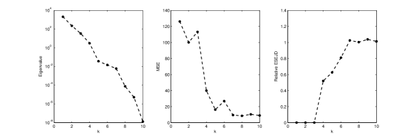
Figure S2: Left panel: Spectrum (up to the first 10 eigenvalues) of the prior-preconditioned Hessian matrix for the one-dimensional image restoration example; Middle: The approximate mean squared error (MSE) in estimating $\mathbb{E}(\boldsymbol{x}\mid\boldsymbol{b})$ versus the rank of the proposal distribution in the LRIS; Right: Approximate expected squared Euclidean jump distance (ESEJD) of the $\boldsymbol{x}$ chain relative to the ESEJD from block Gibbs sampling at convergence.

The middle panel of Figure S2 displays the mean squared errors in the posterior mean estimates versus the rank of the LRIS proposal distribution. We see that the statistical efficiency of the sample mean increases sharply as non-negligible eigenvalues are added to the low-rank approximation, and becomes steady at $k=7$. The right panel of the Figure displays the approximate expected squared Euclidean jumping distance of the Markov chains relative to the average squared jumping distance of the block Gibbs sampler, $\widehat{ESEJD}_{k}/ESEJD_{\text{Gibbs}},~{}k=1,\ldots,10$. Similar to MSE, we can glean that only seven eigenvalues are necessary to obtain within 2,000 iterations a sample whose behavior is equivalent to a converged block Gibbs sampler. This equivalence is further supported in Figure S3, which displays smoothed estimates of the marginal densities of $\mu$ and $\sigma$ as the rank increases. We again see the ability of the LRIS-based algorithm to closely estimate the true marginal density with only 2,000 MCMC iterates. It is interesting to observe that the noise precision $\mu$ is well identified regardless of the rank of the approximation, whereas $\sigma$ is much more difficult to estimate. This reflects identifiability issues that are characteristic of ill-posed Bayesian inverse problems [5].

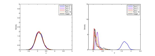
Figure S3: Smoothed approximate marginal posterior densities of the noise precision $\mu$ (left) and prior precision $\sigma$ (right) in the one-dimensional image restoration example. The target density is estimated with the last 1,000 draws from an ordinary block Gibbs sampler with chain length $10^{6}$.

These results demonstrate sharp improvement in the behavior of an LRIS-based MCMC algorithm that is possible when the spectrum of the prior-preconditioned Hessian decays rapidly. Thus, for computationally expensive forward models, there is the potential to dramatically reduce the computational burden without sacrificing the convergence behavior of the Markov chain.

Appendix B Priors on the Nuisance Parameters

Consider the Bayesian linear inverse problem with forward operator $\boldsymbol{A}\in\mathbb{R}^{m\times n}$, assuming independent observations with common precision $\mu$. We assume a Gaussian prior on the target $\boldsymbol{x}$ to correspond to the $L_{2}$ penalty in regularized inversion, with prior covariance matrix $\boldsymbol{\Gamma}_{\text{pr}}$ known up to a multiplicative constant (precision) $\sigma$. Let $\boldsymbol{b}$ denote the observed data. Then the model is

$$\begin{aligned} \boldsymbol{b}\mid\boldsymbol{x},\mu&\sim\mathcal{N}(\boldsymbol{Ax},\mu^{-1}\boldsymbol{I})\\ \boldsymbol{x}\mid\sigma&\sim\mathcal{N}(\boldsymbol{0},\sigma^{-1}\boldsymbol{\Gamma}_{\text{pr}})\\ (\mu,\sigma)&\sim\Pi,\\ \end{aligned}$$ (S1)

where $\Pi$ is some distribution with support $\mathbb{R}^{+}\times\mathbb{R}^{+}$. In the following, we consider two different specifications of $\Pi$.

B.1 Conditionally Conjugate Gamma Priors

The most straightforward case (and by far the most common) is to let $\mu\sim\text{Gamma}(a_{\mu},b_{\mu})$ and $\sigma\sim\text{Gamma}(a_{\sigma},b_{\sigma})$ independently, where we use the shape/rate parameterization of a Gamma distribution; e.g.,

$$\text{Gamma}(\mu\mid a,b)\propto\mu^{a-1}\exp(-b\mu),~{}~{}\mu>0.$$

With these Gamma prior models on $\mu$ and $\sigma$, the joint posterior distribution of the model specified by (S1) is given by

$$\pi(\boldsymbol{x},\mu,\sigma\mid\boldsymbol{b})\propto\mu^{m/2+a_{\mu}-1}\sigma^{n/2+a_{\sigma}-1}\exp\left(-\frac{\mu}{2}\|\boldsymbol{Ax}-\boldsymbol{b}\|^{2}_{2}-\frac{\sigma}{2}\|\boldsymbol{Lx}\|^{2}_{2}-b_{\mu}\mu-b_{\sigma}\sigma\right).$$ (S2)

Since the elements of $\boldsymbol{x}$ are expected to be highly correlated in the posterior, it is desirable to update $\boldsymbol{x}$ all at once in a block Gibbs sampler. The full conditional distributions in this case are

$$\boldsymbol{x}\mid\boldsymbol{b},\mu,\sigma\>\sim \>\mathcal{N}(\boldsymbol{x}_{\text{cond}},\boldsymbol{\Gamma}_{\text{cond}})$$ (S3)

$$\mu\mid\boldsymbol{b},\boldsymbol{x},\sigma\>\sim \>\text{Gamma}\left(m/2+a_{\mu},\frac{1}{2}\|\boldsymbol{Ax}-\boldsymbol{b}\|_{2}^{2}+b_{\mu}\right)$$

$$\sigma\mid\boldsymbol{b},\boldsymbol{x},\mu\>\sim \>\text{Gamma}\left(n/2+a_{\sigma},\frac{1}{2}\|\boldsymbol{Lx}\|_{2}^{2}+b_{\sigma}\right),$$

where $\boldsymbol{\Gamma}_{\text{cond}}=(\mu\boldsymbol{A}^{\top}\boldsymbol{A}+\sigma\boldsymbol{\Gamma}_{\text{pr}}^{-1})^{-1}$ and $\boldsymbol{x}_{\text{cond}}=\mu\boldsymbol{\Gamma}_{\text{cond}}\boldsymbol{A}^{\top}\boldsymbol{b}$. The remaining question becomes specification of the hyperparameters in the Gamma priors.

To impose strong prior assumptions and to stabilize the MCMC algorithm, we can rescale the observed data with $\tilde{\boldsymbol{b}}=\boldsymbol{b}/s_{b}$, where $s_{b}=\sqrt{(m-1)^{-1}\sum_{i=1}^{m}(b_{i}-\overline{b})^{2}}$ is the sample standard deviation. (See, for instance, [31].) In this case, $\mathbb{V}(\tilde{\boldsymbol{b}})$ is expected to be reasonably close to one, though not exactly equal since correlation in the data induced by dependence on $\boldsymbol{x}$ will cause $s_{b}$ to over- or under-estimate the true standard deviation. After rescaling, an equivalent model to (S1) is

$$\tilde{\boldsymbol{b}}=\boldsymbol{A}\tilde{\boldsymbol{x}}+\tilde{\boldsymbol{\epsilon}},$$ (S4)

where $\tilde{\boldsymbol{x}}=\boldsymbol{x}/s_{b}$ and $\tilde{\boldsymbol{\epsilon}}\sim N(\boldsymbol{0},\tilde{\mu}^{-1}\boldsymbol{I})$. This is similar to the notion of a standardized regression model. (See, e.g., [38, Section 7.5].) In this case, we set the hyperparameters in the prior on $\tilde{\mu}$ (or simply $\mu$, without loss of generality) to mildly concentrate the density about one; e.g. $a_{\mu}=b_{\mu}=1$. By concentrating $\mu$ about 1 and allowing $\sigma$ to be vague with, say, $a_{\sigma}=b_{\sigma}=0.1$, we do not strongly restrict values of $\lambda=\sigma/\mu$, the corresponding regularization parameter in the MAP estimator. We remark, however, that in a fully Bayesian model the primary goal is to obtain an estimate of $\boldsymbol{x}$, so we are not really interested in $\mu$ or $\sigma$ in their own right (hence the term “nuisance parameters").

If $\mu\sim\text{Gamma}(\epsilon,\epsilon)$, then $\pi(\mu)\propto\mu^{\epsilon-1}e^{-\epsilon\mu}\rightarrow\mu^{-1}$ as $\epsilon\rightarrow 0$. But $\pi(\mu)=\mu^{-1}$ is the Jeffreys prior for a scale parameter and thus is invariant to reparameterization [9, Ch. 3]. For this reason it is common practice to set $\epsilon$ to some small value in a $\text{Gamma}(\epsilon,\epsilon)$ prior, say $\epsilon=0.1$ or $\epsilon=0.01$, to approximate the behavior of the objective prior without sacrificing propriety or conjugacy. These are the priors we use in the 2D image deblurring example in Section 4.1 of the manuscript.

B.2 Weakly Informative Priors

Despite the convenience associated with the Gamma priors, it was observed by [21] that there is no limiting posterior distribution associated with taking $\epsilon\rightarrow 0$ in a $\text{Gamma}(\epsilon,\epsilon)$ prior, and that using such a hyperprior on the prior-level precision $\sigma$ can sometimes yield undesirable behavior. (Although Carlin and Louis [14] remarked that it may not make a difference in terms of the estimand of interest, $\boldsymbol{x}$.) To rectify this, Gelman [21] proposed as a default prior the folded-t distribution. This prior strikes a good compromise between a completely noninformative prior, which can lead to unreasonable estimates if the data are not informative about a parameter, and a strongly informative prior which prevents the data from ‘speaking for themselves’ in determining plausible a posteriori values. As such, it is called a “weakly informative" prior. Scott and Berger [60] proposed what has since become known as a “proper Jeffreys" prior [48] on the variance components. Defining $\kappa^{2}=\mu^{-1}$ and $\tau^{2}=\sigma^{-1}$, the proper Jeffreys prior takes

$$\pi(\kappa^{2},\tau^{2})=(\kappa^{2}+\tau^{2})^{-2},~{}~{}\kappa^{2},\tau^{2}>0.$$

This prior approximates the improper Jeffreys prior, $\pi(\kappa^{2},\tau^{2})=(\kappa^{2}+\tau^{2})^{-1}$ [65]. Scott and Berger [60] observed that the proper Jeffreys prior can be written as $\pi(\kappa^{2},\tau^{2})=\kappa^{-2}(1+\tau^{2}/\kappa^{2})^{-2}\kappa^{-2}\equiv\pi(\tau^{2}\mid\kappa^{2})\pi(\kappa^{2})$, so that this model is equivalent to using the usual objective prior on the data-level variance while scaling the prior-level variance by $\kappa^{2}$, following the principle originally suggested by Jeffreys [33]. The conditional prior on $\tau^{2}\mid\kappa^{2}$ is also proper, an important consideration in finite mixture models, or when the data contain limited information about $\tau^{2}$. Lastly, it was observed by [11] that the proper Jeffreys prior is tail-equivalent to the prior obtained by placing a folded-$t_{2}$ on $\tau$, and thus is suitable as a default prior choice. For these reasons, this can be an attractive alternative to conjugate Gamma priors. In the CT example in Section 4.2 of the manuscript, we use the proper Jeffreys prior on the variance components. The sampling algorithm is not quite as simple since we no longer have conjugacy (see Appendix B of the manuscript), but we are still able to use our proposed low-rank independence sampler.

Appendix C Non-Centered Parameterizations

In model (S1), the distribution of $\boldsymbol{x}$ depends on $\sigma$, and the distribution of $\boldsymbol{b}$ depends on $\boldsymbol{x}$, but $\boldsymbol{b}$ is conditionally independent of $\sigma$, given $\boldsymbol{x}$. Under Gamma priors on $\mu$ and $\sigma$, this yields convenient conditionally conjugate distributions for use inside a block Gibbs sampler, as discussed in Section B.1 of the Supplementary Material. However, this also leads to high correlation between the $\sigma$ and $\boldsymbol{x}$ chains as the dimension of the problem increases, as noted by Bardsley [5] and Agapiou et al. [1].

A framework for potentially reducing the dependence between parameters in an MCMC algorithm is the so-called non-centered parameterization [45, 46]. A non-centered parameterization is one such that parameters are assigned independent prior distributions but still result in a model equivalent to the usual case, called a centered parameterization. The “centered" and “non-centered" terminology is a reference to the parameterizations considered by [19] for efficient sampling on normal linear mixed models, where certain parameters were centered or non-centered about other parameters.

Papaspiliopoulos et al. [46] argued that the best choice of parameterization depends on how well the underlying parameters are identified by the data. In our case, if the data were significantly informative about $\boldsymbol{x}$ so that strong Bayesian learning occurred in the posterior, then a centered parameterization would likely be appropriate. On the other hand, if $\boldsymbol{x}$ is only weakly identified by the data alone and hence more dependent on prior information, then there tends to be stronger correlation between $\sigma$ and $\boldsymbol{x}$ under the centered parameterization. In this case, a non-centered parameterization is likely the better option. Similar behavior was observed by Agapiou et al. [1], where it was shown that the performance of the non-centered parameterization breaks down as the data-level variance becomes small (i.e., the data become more reliable and thus contain more information about the solution). There exist also “partially non-centered" parameterizations, which can be estimated from the data when the appropriate parameterization to use is not clear [45, 46].

C.1 Implementation

To determine a non-centered parameterization for the hierarchical Bayesian inverse problem, we define a random variable $\boldsymbol{z}$ independent of $\sigma$ and express the distribution of $\boldsymbol{x}$ in terms of these independent random variables. In our case, we have that $\boldsymbol{x}\stackrel{{\scriptstyle\text{d}}}{{=}}\sigma^{-1/2}\boldsymbol{z}$, where $\boldsymbol{z}\sim\mathcal{N}(\boldsymbol{0},\boldsymbol{\Gamma}_{\text{pr}})$ independent of $\sigma$. Substituting this parameterization into (S1), the model becomes

$$\begin{aligned} \boldsymbol{b}\mid\boldsymbol{z},\mu,\sigma&\sim\mathcal{N}(\sigma^{-1/2}\boldsymbol{Az},\mu^{-1}\boldsymbol{I})\\ \boldsymbol{z}&\sim\mathcal{N}(\boldsymbol{0},\boldsymbol{\Gamma}_{\text{pr}})\\ \mu&\sim\text{Gamma}(a_{\mu},b_{\mu})\\ \sigma&\sim\text{Gamma}(a_{\sigma},b_{\sigma}).\end{aligned}$$ (S5)

The joint posterior density is

$$\pi(\boldsymbol{z},\mu,\sigma\mid\boldsymbol{b})\propto f(\boldsymbol{b}\mid\boldsymbol{z},\mu,\sigma)\pi(\boldsymbol{z})\pi(\mu)\pi(\sigma),$$ (S6)

where $f$ is the likelihood, and we adopt the conventional ambiguous use of $\pi$, understood to be defined by its arguments.

The conditional distributions for Gibbs sampling can be derived in a similar manner to the centered case discussed in Section B.1 of the Supplementary Material, with the exception of $\sigma$. The non-centered parameterization loses the conditional conjugacy on this parameter, making an indirect sampling approach necessary. The conditional density of $\boldsymbol{z}$ can be derived as the usual Normal-Normal model $\boldsymbol{b}\sim\mathcal{N}(\boldsymbol{A}_{\sigma}\boldsymbol{z},\mu^{-1}\boldsymbol{I})$ and $\boldsymbol{z}\sim\mathcal{N}(\boldsymbol{0},\boldsymbol{\Gamma}_{\text{pr}})$, where $\boldsymbol{A}_{\sigma}=\sigma^{-1/2}\boldsymbol{A}$. Thus,

$$\boldsymbol{z}\mid\boldsymbol{b},\mu,\sigma\sim\mathcal{N}(\boldsymbol{z}_{\text{cond}},\boldsymbol{\Gamma}_{\text{cond}}),$$

where $\boldsymbol{z}_{\text{cond}}=(\mu\boldsymbol{A}_{\sigma}^{\top}\boldsymbol{A}_{\sigma}+\boldsymbol{L}^{\top}\boldsymbol{L})^{-1}=((\mu/\sigma)\boldsymbol{A}^{\top}\boldsymbol{A}+\boldsymbol{L}^{\top}\boldsymbol{L})^{-1}$ and $\boldsymbol{z}_{\text{cond}}=\mu\boldsymbol{\Gamma}_{\text{cond}}\boldsymbol{A}_{\sigma}^{\top}\boldsymbol{b}=(\mu/\sigma^{1/2})\boldsymbol{\Gamma}_{\text{cond}}\boldsymbol{A}^{\top}\boldsymbol{b}$. One can easily show the same results for this parameterization as in the manuscript with appropriate substitutions of $\mu$ and $\sigma$. In particular, the same simplification of the MH acceptance ratio for the $\boldsymbol{z}$ chain holds as in Proposition 1. The full conditional of $\mu$ is also straightforward. It is derived similarly to the centered case:

$$\pi(\mu\mid\boldsymbol{b},\boldsymbol{z},\sigma) \propto \mu^{m/2+a_{\mu}-1}\exp\left[-\mu\left(\frac{1}{2}\|\boldsymbol{A}_{\sigma}\boldsymbol{z}-\boldsymbol{b}\|_{2}^{2}+b_{\mu}\right)\right]$$

$$\Rightarrow\mu\mid\boldsymbol{b},\boldsymbol{z},\sigma \sim \text{Gamma}\left(m/2+a_{\mu},\frac{1}{2}\|\boldsymbol{A}_{\sigma}\boldsymbol{z}-\boldsymbol{b}\|_{2}^{2}+b_{\mu}\right).$$

The most substantial difference between the centered and non-centered parameterizations is the loss of conditional conjugacy on $\sigma$. The conditional density for $\sigma$ is

$$\pi(\sigma\mid\boldsymbol{b},\boldsymbol{z},\mu)\propto\exp\left[-\frac{\mu}{2}\|\sigma^{-1/2}\boldsymbol{Az}-\boldsymbol{b}\|_{2}^{2}\right]\sigma^{a_{\sigma}-1}e^{-b_{\sigma}\sigma}.$$ (S7)

While there is no obvious simplification or standard distribution for $\sigma$, we can use a random walk Metropolis step to sample from it. Simplifying (S7) slightly, we have

$$\pi(\sigma\mid\boldsymbol{b},\boldsymbol{z},\mu)\propto\sigma^{a_{\sigma}-1}e^{-b_{\sigma}\sigma}\exp\left[-\frac{\mu}{2\sigma}\left(\boldsymbol{z}^{\top}\boldsymbol{A}^{\top}\boldsymbol{Az}-2\sigma^{1/2}\boldsymbol{z}^{\top}\boldsymbol{A}^{\top}\boldsymbol{b}\right)\right],~{}~{}\sigma>0.$$

To eliminate boundary constraints on $\sigma$ and thus facilitate Gaussian proposals in the Metropolis algorithm, reparameterize the model with $\omega=\log(\sigma)$. Then the density for $\omega$ becomes

$$\pi_{\omega}(\omega\mid\boldsymbol{b},\boldsymbol{z},\mu)\propto e^{(a_{\sigma}-1)\omega-b_{\sigma}e^{\omega}}\exp\left[-\frac{\mu}{2}\left(e^{-\omega}\boldsymbol{z}^{\top}\boldsymbol{A}^{\top}\boldsymbol{Az}-2e^{-\omega/2}\boldsymbol{z}^{\top}\boldsymbol{A}^{\top}\boldsymbol{b}\right)\right].$$

To implement the Metropolis step inside the block Gibbs algorithm, we can explicitly separate the burn-in phase from the sampling phase. During the first phase, we seek a suitable proposal distribution for $\sigma$ (i.e., a suitable Gaussian proposal for $\omega$). This is done by adaptively controlling the variance $c$, adjusting its scale based on the acceptance rate of the $\sigma$ samples. A skeleton of this procedure is as follows:

1. Initialize $c=c_{0}$ and $accept=0$.

2. For $i\in$ (burn-in iterations)

   1. Draw $\omega^{\ast}\sim N(\omega^{(i-1)},c)$

   2. Accept/reject $\omega^{\ast}$ according to the Metropolis ratio. If accepted, $accept\leftarrow accept+1$.

   3. If $\mod(i,100)=0$, then

      1. If $accept/100<0.35,~{}c\leftarrow 0.75c$,

      2. Else, if $accept/100>0.5,~{}c\leftarrow 1.75c$

      3. $accept\leftarrow 0$

   4. Repeat

3. For $i\in$ (sampling iterations)

   1. Draw $\omega^{\ast}\sim N(\omega^{(i-1)},c)$, where $c$ is fixed at the value determined from the burn-in period.

   2. Accept/reject $\omega^{\ast}$ according to the Metropolis ratio.

   3. Repeat

Agaipiou et al. [1] also considered a non-centered parameterization in a Bayesian Gaussian linear inverse problem, similar to that considered in this work. They relied on Metropolis sampling, but with a different proposal mechanism. Instead of sampling $\sigma$ directly, they considered $\zeta:=\sigma^{-1/2}$. After a change of variables, the full conditional distribution of $\zeta$ is

$$\pi(\zeta\mid\boldsymbol{b},\boldsymbol{z},\mu) \propto f(\boldsymbol{b}\mid\boldsymbol{z},\mu,\zeta)\pi(\zeta)$$

$$\propto \exp\left[-\frac{\mu}{2}(\boldsymbol{b}-\zeta\boldsymbol{Az})^{\top}(\boldsymbol{b}-\zeta\boldsymbol{Az})\right]\left(\frac{1}{\zeta^{2}}\right)^{a_{\sigma}+1/2}e^{-b_{\sigma}/\zeta^{2}}.$$

We see that the likelihood contribution to this density, written as a function of $\zeta$, is proportional to a Gaussian density. That is,

$$g(\zeta):=\exp\left[-\frac{\mu}{2}(\boldsymbol{b}-\zeta\boldsymbol{Az})^{\top}(\boldsymbol{b}-\zeta\boldsymbol{Az})\right]\propto\exp\left[-\frac{\mu\boldsymbol{z}^{\top}\boldsymbol{A}^{\top}\boldsymbol{Az}}{2}\left(\zeta-\frac{\boldsymbol{z}^{\top}\boldsymbol{A}^{\top}\boldsymbol{b}}{\boldsymbol{z}^{\top}\boldsymbol{A}^{\top}\boldsymbol{Az}}\right)^{2}\right],$$ (S8)

which is the density of a normal distribution with mean $\zeta_{c}:=\boldsymbol{z}^{\top}\boldsymbol{A}^{\top}\boldsymbol{b}(\boldsymbol{z}^{\top}\boldsymbol{A}^{\top}\boldsymbol{Az})^{-1}$ and variance $\xi_{c}:=(\mu\boldsymbol{z}^{\top}\boldsymbol{A}^{\top}\boldsymbol{Az})^{-1}$. Agaipiou et al. [1] use this Gaussian distribution as a proposal for an independence sampler, except that $\zeta$ is restricted to be positive. In other words, their proposal distribution is a truncated Gaussian with density

$$q(\zeta^{\ast})=\mathcal{N}\left(\zeta^{\ast}\mid\zeta_{c},\xi_{c}\right)\left(1-\Phi(-\zeta_{c}/\sqrt{\xi_{c}})\right)^{-1},$$

where $\Phi(\cdot)$ is the cumulative distribution function of the standard normal distribution. It is important to note that this approach assumes $\boldsymbol{A}$ is of full rank, so that $\boldsymbol{Az}\neq\boldsymbol{0}$ for all $\boldsymbol{z}~{}(a.e.)$. In cases where $\boldsymbol{A}$ is rank deficient, one can use the random walk Metropolis step previously discussed, but other approaches are possible.

C.2 Illustration with Image Deblurring

To illustrate use of the non-centered parameterization in our proposed LRIS algorithm, we consider again the 2D image deblurring example from Section 4.1 of the manuscript. Here, the target image $\boldsymbol{x}$ and the blurring operator $\boldsymbol{A}$ are the same as before. However, we create two different observed datasets $\boldsymbol{b}_{i}=\boldsymbol{Ax}+\boldsymbol{\epsilon}_{i},~{}~{}i=1,2$, with two different levels of noise. One set is strongly corrupted with 50% noise, $Var(\boldsymbol{\epsilon}_{1})=0.5^{2}\|\boldsymbol{b}\|_{\infty}^{2}\boldsymbol{I}$, and the other contains much less noise, $Var(\boldsymbol{\epsilon}_{2})=0.01^{2}\|\boldsymbol{b}\|_{\infty}^{2}\boldsymbol{I}$, and thus is more informative about the true solution $\boldsymbol{x}$. The target image, blurred image, and noisy data sets are displayed in Figure S4.

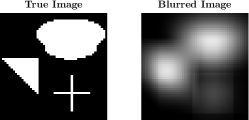
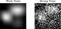
Figure S4: From left to right: target image, blurred image, reliable data, and corrupted data, used for comparing noncentered and centered parameterizations under low-rank independence sampling for 2D deblurring.

For the centered parameterization, we use the same priors on $\boldsymbol{x},\mu$ and $\sigma$ in model (S1) as in the manuscript, namely $\boldsymbol{\Gamma}_{\text{pr}}^{-1}=\boldsymbol{L}^{\top}\boldsymbol{L}$ with $\boldsymbol{L}=-\Delta+\delta\boldsymbol{I}$ and $\epsilon=0.1$ in the $\text{Gamma}(\epsilon,\epsilon)$ priors on $\mu$ and $\sigma$ to approximate scale invariant objective priors. We use the same low-rank Metropolis-Hastings-within-Gibbs algorithm as in the manuscript. To implement the non-centered parameterization, we use our proposed low-rank independent sampler to update $\boldsymbol{x}$ and the independent sampler proposed by [1] to update $\sigma^{-1/2}$. Our interest here is not in posterior inference about the target image, but in the mixing behavior of these two parameterizations applied to data with different amounts of noise. Thus, rather than running to and diagnosing convergence, we run only 5,000 iterations of each Markov chain to study autocorrelation and how quickly the chains appear to be moving through their support. Under each configuration, we run three chains in parallel, with $\mu$ and $\boldsymbol{x}$ initialized by drawing them randomly from their prior distributions. The prior precision $\sigma$ is initialized at $0.1,6$, and $25$ for chains 1, 2, and 3, respectively.

Figure S5 displays the trace plots of the three $\sigma$ chains under each of the four combinations of data and parameterization. With severely noisy data, the noncentered parameterization shows stronger mixing than the centered parameterization. The opposite is true with the reliable data containing only 1% noise. The differences under the reliable data are particulary striking, where we see improvement in the centered paramterization but a very severe degradation in performance of the noncentered parameterization. The drift in all of the chains is indicative of considerable autocorrelation, and this is confirmed by examining the autocorrelation functions plotted in Figure S6 and the estimated lag 1 and lag 50 correlation coefficients in Table S1. Each chain suffers from high lag 1 autocorrelation, but it decays faster under the non-centered parameterization for the noisy data, and faster for the centered parameterization under the more reliable data. The decay of the autocorrelation is particularly poor for the noncentered parameterization with the reliable data.

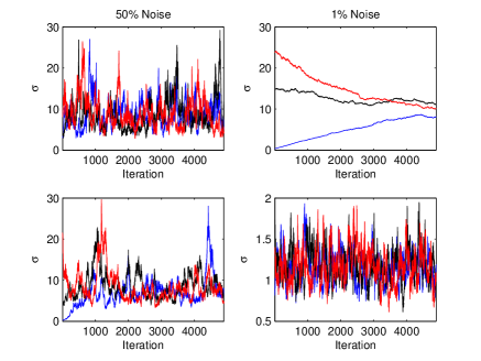
Figure S5: Trace plots of the $\sigma$ chains obtained from centered and non-centered parameterizations using both datasets displayed in Figure S4. The left column corresponds to the noisy data and right column to the reliable data. The top row are plots obtained from the noncentered parameterization, and the bottom row is obtained from the centered parameterization.

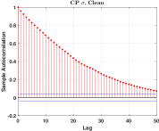
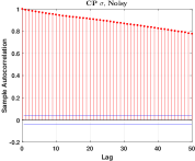
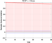
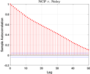
Figure S6: Estimated autocorrelation functions of one $\sigma$ chain from the Supplementary 2D deblurring simulation study, each obtained from centered (top row) and non-centered (bottom row) parameterizations using both weakly (left column) and strongly (right column) corrupted data.

	Reliable		Noisy
	Lag 1	Lag 50	Lag 1	Lag 50
CP	0.968	0.174	0.995	0.774
NCP	0.999	0.974	0.982	0.348

Table S1: Estimated autocorrelation coefficients of one $\sigma$ chain, for each data / parameterization combination in Supplementary simulation study.

The results of this illustration demonstrate the ease with which either the non-centered or centered parameterization can be used in combination with our proposed LRIS. Further, the relative performance of non-centered versus centered parameterizations previously observed in [45, 46, 1] is still present when using our more computationally efficient alternative. In particular, for strongly corrupted data, $\boldsymbol{x}$ is more strongly determined through the prior than the data, so that a non-centered parameterization is preferable. More reliable data impose the constraint that $\boldsymbol{b}\approx\sigma^{-1/2}\boldsymbol{Az}$, severely degrading the performance of the non-centered parameterizaton. Thus, when using our proposed approach, a practitioner can still appeal to the same considerations when choosing a more effective parameterization for convergence of their MCMC algorithm.

Appendix D Adaptive LRIS

The target rank $k$ for the low-rank approximation may not be known in practice, or may depend explicitly on the parameters $\mu$ and $\sigma$. Here we outline a simple adaptive strategy for determining the target rank. The basic idea is to increment the rank till the acceptance ratio meets the desired tolerance.

1. Inputs: user defined tolerance $\delta$, initial rank $k_{\text{init}}$, rank increment $k_{\text{inc}}$

2. Start $k=k_{\text{init}}$

3. While not converged

4. Check if acceptance ratio is higher than $1-\delta$. If, yes, mark converged.

5. Increment the rank $k\leftarrow k+k_{\text{inc}}$.

6. End While

Monitoring the acceptance ratio is important to determine a stopping criterion for the algorithm described above. We suggest several different strategies:

1. The acceptance ratio can be monitored empirically as the independence sampler is exploring the distribution. If the acceptance ratio is too small, the target rank may be incremented.

2. In the case that the exact eigenpairs are used, we derive a lower bound for $w(\boldsymbol{x})$. From the proof of Theorem 1, we find that if $\widehat{\boldsymbol{H}}=\boldsymbol{V}_{k}\boldsymbol{\Lambda}_{k}\boldsymbol{V}_{k}^{\top}$

   $$w(\boldsymbol{x})\geq\exp\left(-\frac{\mu}{2}\|\boldsymbol{Lx}\|_{2}^{2}\|\boldsymbol{H}-\widehat{\boldsymbol{H}}\|_{2}\right)=\exp\left(-\frac{\mu\lambda_{k+1}}{2}\|\boldsymbol{Lx}\|_{2}^{2}\right).$$

   Here $\lambda_{k+1}$ is the largest eigenvalue that is discarded. This suggests that the target rank $k$ is the minimum index which satisfies

   $$\lambda_{k+1}\leq\frac{2}{\mu\|\boldsymbol{Lx}\|_{2}^{2}}\log\frac{1}{1-\delta}.$$

   This will ensure $w(\boldsymbol{x})\geq 1-\delta$, where $\delta$ is a user-defined parameter. It is worth mentioning that the entire eigendecomposition need not be computed, nor recommended. In practice, the eigenpairs can be computed in an incremental fashion.

3. In the randomized low-rank approach, $\lambda_{k+1}$ may not be available. However, it may be easy to estimate $\|\boldsymbol{H}-\widehat{\boldsymbol{H}}\|_{2}$ cheaply using a randomized estimator; see [26, Lemma 4.1]. Then to ensure that $w(\boldsymbol{x})\geq 1-\delta$, it is required that $\|\boldsymbol{H}-\widehat{\boldsymbol{H}}\|_{2}\leq\varepsilon$, where $\varepsilon$ satisfies

   $$\varepsilon\leq\frac{2}{\mu\|\boldsymbol{Lx}\|_{2}^{2}}\log\frac{1}{1-\delta}.$$

   The low-rank approximation can be adaptively and efficiently determined using the adaptive range finding algorithm, see [26, Algorithm 4.2].

Appendix E NMR Relaxometry Simulation

In this section, we investigate the performance of our approach on a large-scale ill-posed inverse problem with a different low-rank nature than the CT example. We consider the problem of nuclear magnetic resonance (NMR) relaxometry in which nuclear magnetic moments are used to infer physical or chemical properties of a medium. The deterioration (or relaxation) of the signal over time is analyzed using various electromagnetic pulse sequences and acquisition strategies. The longitudinal and traverse relaxation times of the medium, denoted $T_{1}$ and $T_{2}$, respectively, can be recovered from these acquisitions. The goal of 2D NMR relaxometry is to reconstruct the joint distribution of the relaxation times, $f(T_{1},T_{2})$, from measured signals gathered at different experimental times, denoted $g(\tau_{1},\tau_{2})$. Mathematically, the forward model is a Fredholm integral equation of the first kind, $g(\tau_{1},\tau_{2})=\int_{0}^{\hat{T}_{2}}\int_{0}^{\hat{T}_{1}}K(\tau_{1},\tau_{2},T_{1},T_{2})f(T_{1},T_{2})\,\mathrm{d}T_{1}\mathrm{d}T_{2}.$ As in the 1D image deblurring example, the measurement noise is typically assumed to be Gaussian and the problem is to reconstruct $f$ from $g$ and $K$.

We use the implementation in the Matlab package IR Tools [18] to simulate NMR data. In this example, the kernel is separable, and after discretization we obtain the linear inverse problem $\boldsymbol{Ax}=\boldsymbol{b}$, where $\boldsymbol{b}$ is the vectorization of the data $g$ and $\boldsymbol{x}$ the vectorization of the unknown $f$. Unlike the other examples we consider in this work, the forward map $\boldsymbol{A}$ and its transpose are not constructed explicitly, but their matrix-vector products are computed using available function handles. We again enforce smoothness in $\boldsymbol{x}$ by specifying $\boldsymbol{L}=-\Delta+\delta\boldsymbol{I}$ and corrupt the data with one percent Gaussian random noise. With the default discretizations, the data have dimension $m=65,536$ and the unknown has dimension $n=16,384$. The noisy data $\boldsymbol{b}$ and unknown $\boldsymbol{x}$ are displayed in Figure S7. We compute approximate eigenvalues of the prior preconditioned Hessian using Randomized SVD with $\ell=1000$. The sharp decay in the eigenvalues, also displayed in Figure S7, illustrates the severe ill-posedness of the NMR relaxometry inverse problem.

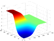
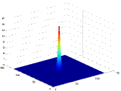
Figure S7: Noisy measured data $\boldsymbol{b}$ (left) and true relaxation distribution $\boldsymbol{x}$ (center) in the NMR relaxometry example. Approximate spectrum of $\boldsymbol{H}$ (right) shows significant decay within the first few hundred eigenvalues.

For implementation, we perform the same experiment as in Section 4.2 of the manuscript with the same vague conjugate Gamma priors on $\mu$ and $\sigma$. Analyzing the acceptance rates for different eigenvalue truncation levels as well as the spectral decay in Figure S7, we specify the truncation level $k=300$ (average acceptance rate $\approx 100\%$). We simulate three Markov chains for 40,000 iterations each, initializing each chain with random draws from the priors. To reduce the autocorrelation in the chains, they are thinned to retain every 50th draw, after which the first 400 draws are discarded as the burn-in period. Approximate convergence of the chains is diagnosed via trace plots and autocorrelation plots, displayed in Figures S8 and S9. The PSRFs for $\mu$ and $\sigma$ are 0.99 and 1.01, respectively. The computations are carried out in MATLAB 2013a on a Dell Precision T3600 desktop PC running Windows 7 Enterprise with an Intel Xeon E5-1660 3.30GHz CPU and 64GB RAM. The total computation time is 13,263 seconds, or about 3.7 hours.

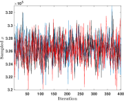
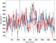
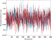
Figure S8: Trace plots for the three thinned chains using Gamma priors in the NMR relaxometry example. Left: noise precision $\mu$. Center: prior precision $\sigma$. Right: a randomly chosen pixel of the image $\boldsymbol{x}$.

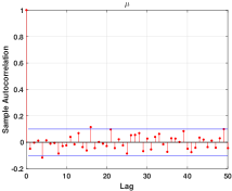
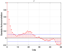
Figure S9: Autocorrelation plots for one thinned chain using Gamma priors in the NMR relaxometry example. Left: noise precision $\mu$. Right: prior precision $\sigma$.

Figure S10 displays the posterior mean of $\boldsymbol{x}$ based upon the output of the MCMC at approximate convergence, as well as the approximate densities of $\mu$ and $\sigma$. While we obtain a reasonable estimate of the distribution of relaxation times, it is strongly attenuated compared to the true solution and exhibits background fluctuations (including negative values). The attenuation, though, is similar to the solution obtained in [18] via conjugate gradient least squares, though our posterior mean produces a smoother estimate. Indeed, [18] remark that the NMR problem is extremely challenging and that even the iterative methods they consider require many thousands of iterations to produce interpretable estimates of $\boldsymbol{x}$.

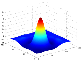
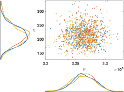
Figure S10: Posterior mean estimate of $\boldsymbol{x}$ (left) and smoothed histograms of $\mu$ and $\sigma$ (right) in the NMR relaxometry example.

Our low-rank approach offers considerable computational advantages over standard MCMC, thus making it feasible to reconstruct a competitive solution along with appropriate measures of uncertainty. It is demonstrated in [18] that non-negativity constraints on $\boldsymbol{x}$ can yield an improved solution. In our framework, this suggests that a truncated Gaussian or lognormal prior on $\boldsymbol{x}$ may produce solutions superior to that produced by the Gaussian prior. Such an investigation is beyond the scope of this work and left for future research.

Appendix F Supplementary Figures

In Supplementary Figure S11, we compare the (vague) Gamma priors on $\mu$ and $\sigma$ with the marginal posterior distributions estimated from the MCMC samples of the joint posterior. The prior for $\mu$ has been scaled by a factor of 10,000 for visualization. Note the significant difference between the distributions, indicating that strong Bayesian learning has occurred.

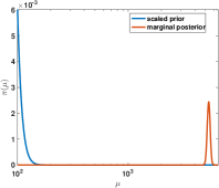
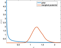
Figure S11: Priors and marginal posterior distributions for $\mu$ (left) and $\sigma$ (right) in the 2D deblurring example.

Trace plots of the samples from the thinned MCMC chains using weakly informative priors in the CT example (Section 4.2) are displayed in Supplementary Figure S12, and autocorrelation plots are displayed in Supplementary Figure S13. In Supplementary Figure S14, we plot the cumulative averages of the parameters $\kappa^{2}$ and $\upsilon$ of these samples. The PSRFs for these parameters were both 1.00. Even after thinning, we see some correlation between the samples.

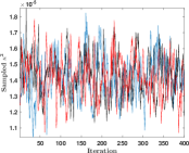
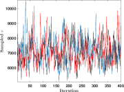
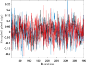
Figure S12: Trace plots for the thinned chains in the CT image reconstruction example. Left: noise variance $\kappa^{2}$. Center: Variance ratio $\upsilon=\tau^{2}/\kappa^{2}$. Right: A randomly chosen pixel of the image $\boldsymbol{x}$.

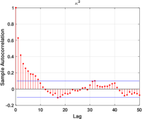
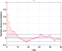
Figure S13: Autocorrelation plots for the thinned chains in the CT image reconstruction example. Left: noise variance $\kappa^{2}$. Right: Variance ratio $\upsilon=\tau^{2}/\kappa^{2}$.

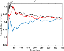
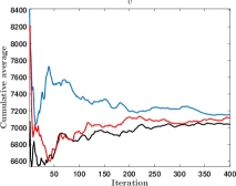
Figure S14: Cumulative averages of $\kappa^{2}$ and $\upsilon$ for each of the thinned MCMC chains in the CT example.

We next present convergence diagnostics for the CT example with the conjugate Gamma prior instead of proper Jeffreys to justify the comparison in the manuscript. We use vague Gamma priors for $\mu$ and $\sigma$ as in the 2D example, and the same prior for $\boldsymbol{x}$ as in the original CT experiment. We again use Randomized SVD with target rank $\ell=5000$ in the low-rank proposal distribution for $\boldsymbol{x}$. We simulate three (randomly initialized) Markov chains using the MCMC algorithm with our proposed approach for 20,000 iterations. These chains are then thinned and the burn-in period discarded to produce an equal Monte Carlo sample size as in the previous experiment. Trace plots, autocorrelation plots, and PSRFs are used to determine approximate convergence of the chains. The trace plots are displayed in Supplementary Figure S15 and the autocorrelation plots for $\mu$ and $\sigma$ are in Supplementary Figure S16. The PSRFs for $\mu$ and $\sigma$ were 1.00 and 1.01 respectively.

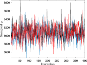
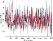
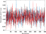
Figure S15: Trace plots for the three thinned chains using Gamma priors in the CT image reconstruction example. Left: noise precision $\mu$. Center: prior precision $\sigma$. Right: a randomly chosen pixel of the image $\boldsymbol{x}$.

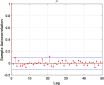
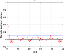
Figure S16: Autocorrelation plots for one thinned chain using Gamma priors in the CT image reconstruction example. Left: noise precision $\mu$. Right: prior precision $\sigma$.

References

- [1] S. Agapiou, J. M. Bardsley, O. Papaspiliopoulos, and A. M. Stuart. Analysis of the Gibbs sampler for hierarchical inverse problems. SIAM/ASA Journal on Uncertainty Quantification, 2(1):511–544, 2014.
- [2] K. E. Andersen, S. P. Brooks, and M. B. Hansen. Bayesian inversion of geoelectrical resistivity data. J. R. Stat. Soc. B., 65(3):619–642, 2003.
- [3] J. M. Bardsley. WMRNSD for medical imaging examples. http://www.math.umt.edu/bardsley/codes.html. Accessed: 2016-06-23.
- [4] J. M. Bardsley. Applications of nonnegatively constrained iterative method with statistically based stopping rules to CT, PET, and SPECT imaging. Electron. Trans. Numer. Ana., 38:34–43, 2011.
- [5] J. M. Bardsley. MCMC-based image reconstruction with uncertainty quantification. SIAM J. Sci. Comput., 34(3):A1316–A1332, 2012.
- [6] J. M. Bardsley, M. Howard, and J. G. Nagy. Efficient MCMC–based image deblurring with Neumann boundary conditions. Electron. Trans. Numer. Ana., 40:476–488, 2013.
- [7] J. M. Bardsley, K. T. Joyce, and A. Luttman. Partially collapsed Gibbs samplers for linear inverse problems and applications to X-ray imaging. Manuscript in submission, 2016.
- [8] J. M. Bardsley and A. Luttman. A Metropolis-Hastings method for linear inverse problems with Poisson likelihood and Gaussian prior. Int. J. Uncertain. Quan., 6(1):35–55, 2016.
- [9] J. O. Berger. Statistical Decision Theory and Bayesian Analysis. Springer-Verlag, New York, 2nd edition, 1985.
- [10] S. P. Brooks and A. Gelman. General methods for monitoring convergence of iterative simulations. J. Comput. Graph. Stat., 7(4):434–455, 1998.
- [11] D. A. Brown, G. S. Datta, and N. A. Lazar. A Bayesian generalized CAR model for correlated signal detection. Stat. Sinica, 27:1125–1153, 2017.
- [12] T. Bui-Thanh, O. Ghattas, J. Martin, and G. Stadler. A computational framework for infinite-dimensional Bayesian inverse problems part i: The linearized case, with application to global seismic inversion. SIAM J. Sci. Comput., 35(6):A2494–A2523, 2013.
- [13] D. Calvetti, J. P. Kaipio, and E. Somersalo. Inverse problems in the Bayesian framework. Inverse Probl., 30(11), 2014.
- [14] B. P. Carlin and T. A. Louis. Bayesian Methods for Data Analysis. Chapman & Hall/CRC, Boca Raton, 3rd edition, 2009.
- [15] R. V. Craiu and X.-L. Meng. Perfection within reach: Exact MCMC sampling. In S. Brooks, A. Gelman, G. L. Jones, and X.-L. Meng, editors, Handbook of Markov Chain Monte Carlo, pages 199–226. Chapman & Hall/CRC Press, 2011.
- [16] H. P. Flath, L. C. Wilcox, V. Akçelik, J. Hill, B. van Bloemen Waanders, and O. Ghattas. Fast algorithms for Bayesian uncertainty quantification in large-scale linear inverse problems based on low-rank partial Hessian approximations. SIAM J. Sci. Comput., 33(1):407–432, 2011.
- [17] C. Fox and R. A. Norton. Fast sampling in a linear–Gaussian inverse problem. SIAM/ASA Journal on Uncertainty Quantification, 4:1191–1218, 2016.
- [18] S. Gazzola, P. C. Hansen, and J. G. Nagy. Ir tools: A matlab package of iterative regularization methods and large-scale test problems. arXiv preprint arXiv:1712:05602, 2017.
- [19] A E Gelfand, S K Sahu, and B P Carlin. Efficient parameterisations for normal linear mixed models. Biometrika, 82(3):479–488, 1995.
- [20] A. E. Gelfand and A. F. M. Smith. Sampling-based approaches to calculating marginal densities. J. Am. Stat. Assoc., 85(410):398–409, 1990.
- [21] A. Gelman. Prior distributions for variance parameters in hierarchical models. Bayesian Anal., 1(3):515–533, 2006.
- [22] A. Gelman, J. B. Carlin, H. S. Stern, D. B. Dunson, A. Vehtari, and D. B. Rubin. Bayesian Data Analysis. Chapman & Hall/CRC, Boca Raton, 3rd edition, 2014.
- [23] A. Gelman, G. Roberts, and W. Gilks. Efficient Metropolis jumping rules. In J. M. Bernardo, J. O. Berger, A. P. Dawid, and A. F. M. Smith, editors, Bayesian Statistics 5, volume 5, pages 599–607. Oxford University Press, New York, 1995.
- [24] A. Gelman and D. B. Rubin. Inference from iterative simulation using multiple sequences (with discussion). Stat. Sci., 7:457–511, 1992.
- [25] S. Geman and D. Geman. Stochastic relaxation, Gibbs distributions and the Bayesian restoration of images. IEEE T. Pattern Anal., 6:721–741, 1984.
- [26] N. Halko, P. G. Martinsson, and J. A. Tropp. Finding structure with randomness: Probabilistic algorithms for constructing approximate matrix decompositions. SIAM Rev., 53(2):217–288, 2011.
- [27] P. C. Hansen. Regularization tools version 4.0 for Matlab 7.3. Numer. Algorithms, 46:189–194, 2007.
- [28] P. C. Hansen. Discrete inverse problems: Insight and algorithms, volume 7. SIAM, 2010.
- [29] W. Hastings. Monte Carlo sampling methods using Markov chains and their application. Biometrika, 57:97–109, 1970.
- [30] O. Hauk. Keep it simple: A case for using classical minimum norm estimation in the analysis of EEG and MEG data. NeuroImage, 21:1612–1621, 2004.
- [31] D. Higdon, J. Gattiker, B. Williams, and M. Rightley. Computer model calibration using high-dimensional output. J. Am. Stat. Assoc., 103:570–583, 2008.
- [32] R. A. Horn and C. R. Johnson. Topics in Matrix Analysis. Cambridge University Press, Cambridge, 1991.
- [33] H. Jeffreys. Theory of Probability. Oxford University Press, Cambridge, 3rd edition, 1961.
- [34] A. Johnson, G. L. Jones, and R. C. Neath. Component-wise Markov chain Monte Carlo: Uniform and geometric ergodicity under mixing and composition. Stat. Sci., 28(3):360–375, 2013.
- [35] R. A. Johnson and D. W. Wichern. Applied Multivariate Statistical Analysis. Prentice Hall, Upper Saddle River, 6th edition, 2007.
- [36] M. Jordan, Z. Ghahramani, T. Jaakkola, and L. Saul. Introduction to variational methods for graphical models. Mach. Learn., 37(1):183–233, 1999.
- [37] J. Kaipio and E. Somersalo. Statistical and Computational Inverse Problems. Springer, New York, 2005.
- [38] Kutner, M. and Nachtsheim, C. and Neter, J. and Li, W. Applied Linear Statistical Models. McGraw-Hill/Irwin, Boston, 5th edition, 2005.
- [39] J. S. Liu. Metropolized independent sampling with comparisons to rejection sampling and importance sampling. Stat. Comput., 6:113–119, 1996.
- [40] J. S. Liu, W. H. Wong, and A. Kong. Covariance structure of the Gibbs sampler with applications to the comparisons of estimators and augmentation schemes. Biometrika, 84:27–40, 1994.
- [41] N. Metropolis, A. W. Rosenbluth, M. N. Rosenbluth, A. H. Teller, and E. Teller. Equation of state calculations by fast computing machines. J. Chem. Phys., 21:1087–1091, 1953.
- [42] K. Mosegaard and A. Tarantola. Probabilistic approach to inverse problems. In International Handbook of Earthquake & Engineering Seismology, Part A., pages 237–265. Academic Press, 2002.
- [43] P. Müller. A generic approach to posterior integration and Gibbs sampling. Technical Report, Purdue University, 1991.
- [44] C. Nahkhleh, D. Higdon, C. K. Allen, and R. Ryne. Bayesian reconstruction of particle beam phase space. In Bayesian Theory and Applications, pages 673–686. Oxford University Press, 2013.
- [45] O. Papaspiliopoulos and G. O. Roberts. Non-Centered Parameterisations for Hierarchical Models and Data Augmentation. Bayesian Statistics, 7:307–326, 2003.
- [46] O. Papaspiliopoulos, G. O. Roberts, and M. Sköld. A General Framework for the Parametrization of Hierarchical Models. Stat. Sci., 22(1):59–73, 2007.
- [47] N. Petra, J. Martin, G. Stadler, and O. Ghattas. A computational framework for infinite-dimensional Bayesian inverse problems, part ii: Stochastic Newton MCMC with application to ice sheet flow inverse problems. SIAM J. Sci. Comput., 36(4):A1525–A1555, 2014.
- [48] N. G. Polson and J. G. Scott. Shrink globally, act locally: Sparse Bayesian regression and prediction. In J. M. Bernardo, M. J. Bayarri, J. O. Berger, A. P. Dawid, D. Heckerman, A. F. M. Smith, and M. West, editors, Bayesian Statistics 9, pages 501–538. Oxford University Press, 2010.
- [49] P. Z. G. Qian and C. F. J. Wu. Bayesian hierarchical modeling for integrating low-accuracy and high-accuracy experiments. Techometrics, 50:192–204, 2008.
- [50] C. E. Rasmussen and C. K. I. Williams. Gaussian Processes for Machine Learning. MIT Press, Cambridge, 2006.
- [51] S. I. Resnick. A Probability Path. Birkhäuser, Boston, 1999.
- [52] C. Robert and G. Casella. Monte Carlo Statistical Methods. Springer, New York, 2nd edition, 2004.
- [53] J. S. Rosenthal. Optimal proposal distributions and adaptive MCMC. In S. Brooks, A. Gelman, G. L. Jones, and X.-L. Meng, editors, Handbook of Markov Chain Monte Carlo, pages 93–111. Chapman & Hall/CRC, Boca Raton, 2011.
- [54] H. Rue and L. Held. Gaussian Markov Random Fields. Chapman & Hall/CRC, Boca Raton, 2005.
- [55] H. Rue, S. Martino, and N. Chopin. Approximate Bayesian inference for latent Gaussian models by using integrated nested Laplace approximations. J. R. Stat. Soc. B., 71(2):319–392, 2009.
- [56] Y. Saad. Numerical Methods for Large Eigenvalue Problems, volume 158. SIAM, 1992.
- [57] A. K. Saibaba and P. K. Kitanidis. Fast computation of uncertainty quantification measures in the geostatistical approach to solve inverse problems. Adv. Water Resour., 82(0):124–138, 2015.
- [58] A. K. Saibaba, J. Lee, and P. K. Kitanidis. Randomized algorithms for generalized Hermitian eigenvalue problems with application to computing Karhunen–Loève expansion. Numer. Linear Algebr., 23(2):314–339, 2016.
- [59] T. J. Santner, B. J. Williams, and W. I. Notz. The Design and Analysis of Computer Experiments. Springer-Verlag, New York, 2003.
- [60] J. G. Scott and J. O. Berger. An exploration of aspects of Bayesian multiple testing. J. Stat. Plan. Infer., 136(7):2144–2162, 2006.
- [61] C. B. Shaw. Improvements of the resolution of an instrument by numerical solution of an integral equation. J. Math. Anal. Appl., 37:83–112, 1972.
- [62] L. A. Shepp and B. F. Logan. The Fourier reconstruction of a head section. IEEE T. Nucl. Sci., 21(3):21–43, 1974.
- [63] A. Spantini, A. Solonen, T. Cui, J. Martin, L. Tenorio, and Y. Marzouk. Optimal low-rank approximations of Bayesian linear inverse problems. SIAM J. Sci. Comput., 37(6):A2451–A2487, 2015.
- [64] A. M. Stuart. Inverse problems : A Bayesian perspective. Acta Numer., 19(May):451–559, 2010.
- [65] G. C. Tiao and W. Tan. Bayesian analysis of random-effect models in the analysis of variance, I. Posterior distribution of variance components. Biometrika, 51:37–53, 1965.
- [66] J. A. Tropp, A. Yurtsever, M. Udell, and V. Cevher. Randomized single-view algorithms for low-rank matrix approximation. arXiv preprint arXiv:1609.00048, 2016.
- [67] van Dyk, D. and Park, T. Partially collapsed Gibbs samplers. J. Am. Stat. Assoc., 103:790–796, 2008.
Supplementary Material for Low Rank Independence Samplers in Bayesian Inverse Problems
D. Andrew Brown Arvind Saibaba Sarah Vallélian