Blind Detection of Ultra-faint Streaks with a Maximum Likelihood Method

Abstract

We have developed a maximum likelihood source detection method capable of detecting ultra-faint streaks with surface brightnesses approximately an order of magnitude fainter than the pixel level noise. Our maximum likelihood detection method is a model based approach that requires no a priori knowledge about the streak location, orientation, length, or surface brightness. This method enables discovery of typically undiscovered objects, and enables the utilization of low-cost sensors (i.e., higher-noise data). The method also easily facilitates multi-epoch co-addition. We will present the results from the application of this method to simulations, as well as real low earth orbit observations.

Introduction

Satellites and near earth objects (NEOs) appear as streaks in the images of sidereal tracking surveys. There is evidence that the NEOs and satellites (including space debris) follow an inverse power law luminosity function with there being many more fainter objects than brighter objects [11, 10, 1]. Thus going fainter provides the best return on object characterization and actionable information. Additionally, algorithms that can detect streaks as faint as possible can enable the use of lower cost telescopes and detectors.

Astronomical surveys of local solar system or Earth orbiting objects typically fall into two broad categories: object tracking and sidereal tracking. In the case of object tracking, the object of interest will appear as a point source convolved with the atmospheric/optic point spread function (PSF) and the stars or other objects moving at a different angular velocity will appear as streaks. In the case of sidereal tracking, the stars will appear as PSF’s and satellites and NEOs will appear as streaks of varying lengths. Sidereal tracking surveys have the advantage of enabling easy discrimination of satellites and NEOs from galactic and extra-galactic sources, which significantly outnumber the satellites and NEOs. This comes at the price of making detection of satellites and NEOs more challenging due to extending their signal spatially and increasing the noise floor as a function of the angular velocity of the source [8]. We will introduce a maximum likelihood detection method as a statistically rigorous extension of a signal-matched-filter [19, 17] that is capable of maximizing the detectability of satellites and NEOs in both categories of surveys while maintaining high purity.

Method

In general, a signal-matched-filter will maximize the detectability of a given object. In the case of a ground-based object tracking survey the signal matched filter is the PSF, and in the case of a sidereal tracking survey it is a finite line convolved with the PSF, see for example the work by [13] presented at this conference or [18, 7, 12]. In addition to incorporating a signal- matched-filter, methods that can account for spatially and temporally varying pixel covariance, facilitate the combination of multiple epochs of images [16], incorporate prior information, and account for pixel level systematics (e.g., aliasing), among other basic image reduction tasks (e.g., flat-fielding, background subtraction, etc.), can further increase the magnitude limit of detectability. The maximum likelihood detection method exemplifies all of these beneficial features and is furthermore statistically sound.

Kaiser developed and discussed in great detail a maximum likelihood detection method for PSF sources as part of the Pan-STARRS survey [4, 5]. In this section we generalize this method to include extended sources and specifically discuss the applicability of the method to detecting streaks. Additionally, we discuss some of the practical considerations in applying this method.

General Form

In this section we derive the general form of the maximum likelihood source detection method. The likelihood of there being a source at location $\mathbf{x}$ in the image plane with properties $\omega$ is,

$$\mathrm{ln}\mathcal{L}\left(\mathbf{x},\omega\right)=-\tfrac{1}{2}\left[d(\mathbf{x})-m(\mathbf{x},\omega)\right]^{\mathrm{T}}\Sigma\left(\mathbf{x},\omega\right)^{-1}\left[d(\mathbf{x})-m(\mathbf{x},\omega)\right]+C,$$ (1)

where $d$ is the pixel data (e.g., analog-to-digital units), $m$ is the source model that can be the convolution of the source $s$ with the PSF $\Pi$,

$$m(\mathbf{x},\omega)=\int s(\mathbf{x},\omega)\Pi(\mathbf{x})\mathrm{d}\mathbf{x},$$ (2)

$\Sigma$ is the pixel covariance, and $C$ is a constant. We can maximize this likelihood with respect to the object flux,

$$m(\mathbf{x},\omega)\equiv\alpha\mu(\mathbf{x},\Omega),$$ (3)

where $\mu$ is a source image model with unity flux, $\alpha$ is a multiplicative scaling of the unit flux, and $\Omega$ is the same as the set $\omega$ but excluding the flux or surface brightness parameter. It is also convenient to expand the likelihood,

$$\mathrm{ln}\mathcal{L}\left(\mathbf{x},\omega\right)=-\tfrac{1}{2}d^{\mathrm{T}}\Sigma^{-1}d-\tfrac{1}{2}m^{\mathrm{T}}\Sigma^{-1}m+d^{\mathrm{T}}\Sigma^{-1}m+C,$$ (4)

and define the functions

$$\Phi(\mathbf{x},\Omega)=\mu(\mathbf{x},\Omega)^{\mathrm{T}}\Sigma^{-1}\mu(\mathbf{x},\Omega),$$ (5)

and

$$\Psi(\mathbf{x},\Omega)=d(\mathbf{x})^{\mathrm{T}}\Sigma^{-1}\mu(\mathbf{x},\Omega).$$ (6)

These are the noise weighted model auto-correlation, and noise weighted data-model cross-correlation, respectively. In these terms the maximum likelihood can be solved for with

$$\frac{\partial\mathrm{ln}\mathcal{L}}{\partial\alpha}=\alpha\Phi(\mathbf{x},\Omega)-\Psi(\mathbf{x},\Omega)=0.$$ (7)

Solving Equation 7 we see that the maximum likelihood flux of the model object at position $\mathbf{x}$ is

$$\alpha_{\mathrm{ML}}=\frac{\Psi(\mathbf{x},\Omega)}{\Phi(\mathbf{x},\Omega)},$$ (8)

and the maximum likelihood is,

$$\mathrm{ln}\mathcal{L}_{\mathrm{ML}}=\frac{\Psi^{2}(\mathbf{x},\Omega)}{2\Phi(\mathbf{x},\Omega)}.$$ (9)

Given this we can express the significance of there being an object at location $\mathbf{x}$ with properties $\Omega$ as

$$\nu(\mathbf{x},\Omega)=\frac{\Psi(\mathbf{x},\Omega)}{\sqrt{\Phi(\mathbf{x},\Omega)}}.$$ (10)

There are a number of beneficial features associated with this method. If we wish to combine multiple epochs we simply need to sum the log likelihoods, Equation 9, of the different epochs (see also [3]). For example, if the source moves or if the PSF changes between epochs $i$ and $j$ we can simply sum $\mathrm{ln}\mathcal{L}_{\mathrm{ML}}(\mathbf{x}_{i},\Pi_{i}(\mathbf{x}_{i}),\cdot)+\mathrm{ln}\mathcal{L}_{\mathrm{ML}}(\mathbf{x}_{j},\Pi_{j}(\mathbf{x}_{j}),\cdot)$ and estimate a combined significance of detection. Note that because the coordinates $\mathbf{x}$ need not be integer pixel values, this avoids many systematics associated with working on a pixel grid and obviates the need for complex pixel transformations before co-addition. This also more rigorous than many common co-addition practices, such as convolving to the images taken with better seeing (i.e., smaller PSF) by that of the worst seeing image’s PSF before co- adding data, which throw away information. It is also trivial to incorporate spatially varying source models, image noise, and PSFs.

Streak Model

Since point source models (i.e., $s=\delta(\mathbf{x})$) are more straightforward and have been treated in great detail by Kaiser [4, 5], we will focus on streak models for this report. As detailed in [13], we model a streak in image space as a product of a narrow Gaussian (representing the width that can be made arbitrarily small) and a rectangular window (representing the extent of the streak; see also [18]). We further assume that the streak model is evaluated in a coordinate system with the center of the streak at the origin and the extent of the streak along the x-axis. This can always be accomplished by means of a coordinate translation by $x_{0}$, $y_{0}$ and a rotation by $\phi_{0}$. Then a streak of length $L$, width $\sigma_{y}$, and surface brightness $l_{0}$ (i.e., luminosity per unit area) convolved with a Gaussian approximated PSF with covariance $\sigma^{2}_{\Pi}$ can be modeled as,

$$m=\frac{\ell_{0}}{2}\left[\rm Erf\left(\frac{L-2H_{x}}{2\sqrt{2\sigma_{\Pi}^{2}}}\right)+\rm Erf\left(\frac{L+2H_{x}}{2\sqrt{2\sigma_{\Pi}^{2}}}\right)\right]\exp\left(-\frac{1}{2}\frac{H_{y}^{2}}{\sigma_{\Pi}^{2}+\sigma_{y}^{2}}\right)\frac{\sqrt{2\pi\sigma_{y}^{2}}}{\sqrt{2\pi(\sigma_{\Pi}^{2}+\sigma_{y}^{2})}}$$ (11)

where the streak’s location, $\left(x_{0},y_{0}\right)$, and position angle, $\phi_{0}$, in image space can be described by,

$$\mathbf{H}_{x} =(x-x_{0})\cos\phi_{0}-(y-y_{0})\sin\phi_{0}$$ (12)

$$\mathbf{H}_{y} =(x-x_{0})\sin\phi_{0}+(y-y_{0})\cos\phi_{0}.$$ (13)

For the current consideration of ground-based imaging $\sigma_{y}^{2}\ll\sigma_{\Pi}^{2}$ for this model and can be neglected. Thus our streak model has parameters,

$$\omega\equiv\left[x_{0},y_{0},\phi_{0},\ell_{0},L,\sigma_{\Pi}^{2}\right].$$ (14)

Since we maximize the likelihood with respect to the object flux for detection, Equation 11, we only need to explore the model parameter space,

$$\Omega\equiv\left[x_{0},y_{0},\phi_{0},L,\sigma_{\Pi}^{2}\right],$$ (15)

when detecting streaks.

Practical Matters

While in principle one can incorporate the non- flatness and background of the image into the source model, it is convenient to utilize conventional image reduction procedures to first produce flat fielded and background subtracted images and then run the maximum likelihood source detection on these.

It is also convenient when searching for ultra-faint satellites and NEOs to remove the stars and galaxies from the images before running the maximum likelihood source detection to detect the satellites and NEOs. There are numerous ways to do this. One convenient means, when consecutive images have been taken of the same area of the sky, is median stacking. In the case of object tracking, a median stack can be created which will effectively filter out the star streaks, assuming that the density of stars is low enough and exposure times are short enough that star streaks do not significantly overlap from exposure to exposure. In the case of sidereal tracking, a median stack can be constructed which will filter out all objects that move from exposure to exposure. This median stack can then be subtracted for the individual epochs to leave images with only the moving objects. This is superior to masking procedures which often fail to mask the low surface brightness Airy disk wings of stars that can contribute significantly to false detections when searching for low surface brightness streaks.

In subsection 4.3 we will discuss the practical matter of using the maximum likelihood method to detect multiple streaks of varying properties in a single image, as well as deblending.

Demonstrations of the Method

In this section, we demonstrate the maximum likelihood detection method discussed in section 3 by applying it to simulations and real data. We will focus on the more challenging sidereal tracking case (i.e., detecting streaks). In subsection 4.1, we apply the method to simulated data of a single ultra-faint streak showing details of various phases of the detection pipeline. In subsection 4.2, we show some of the results of applying our method in an unsupervised, or blind, fashion to real data containing a satellite in low earth orbit (LEO). Finally, in subsection 4.3, we demonstrate how multiple objects can be detected in a simulated image containing multiple streaks.

Fig. 1: A sequence of images demonstrating various phases of the maximum likelihood reduction pipeline, section 3. a) We simulated an ultra-faint streak according to our model, Equation 11, between four brighter Gaussian PSF stars. The black line is an annotation to guide the eye to the simulated streak. b) We use a Gaussian PSF model in our maximum likelihood formalism to detect objects with $\nu_{\mathrm{PSF}}>5$ and mask these regions from the $\Psi_{\mathrm{PSF}}$ and $\Phi_{\mathrm{PSF}}$ images. Note that the faint streak is just barely visible, but all portions of it are still below $5\sigma$ significance. c) Since the convolutions are transitive we can operate on the $\Psi_{\mathrm{PSF}}$ and $\Phi_{\mathrm{PSF}}$ images with a simple line model (absent the PSF) to generate c) $\Psi_{\mathrm{streak}}$, d) $\Phi_{\mathrm{streak}}$, and e) $\nu_{\mathrm{streak}}$ images for faint streak detection purposes. f) Shows the faint streak footprint which was detected at more than $10\sigma$ significance.

Simulated Single Ultra-faint Streak

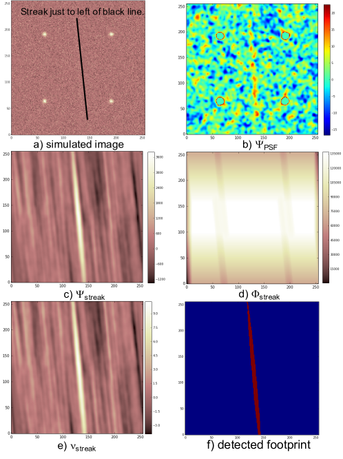
We simulated a ground-based image containing an ultra-faint streak ($l_{0}<$RMS noise) along with four brighter stars, all convolved with a Gaussian PSF, see Figure 1a. We first estimate the PSF, convolve the image with a Gaussian kernel of that width, and using the maximum likelihood detection method, detect objects with significance $\nu_{\mathrm{PSF}}>5$, where $\nu$ is defined in Equation 10. We then refine our PSF estimate empirically based on the detected stars and redo the detection process to generate $\Psi_{\mathrm{PSF}}$, $\Phi_{\mathrm{PSF}}$, and $\nu_{\mathrm{PSF}}$ images. Using percolation theory to identify contiguous pixels in the $\nu$ image above the threshold, we then mask out the pixels associated with star (or bright streaks that were identified after the PSF convolution) from the various PSF images. For example, we show the masked $\Psi_{\mathrm{PSF}}$ image in Figure 1b, where hints of the simulated streak is now apparent but still low significance.

Because convolution operations are transitive we can operate on the PSF convolved images with a simple line model and it is the same as operating on the raw data with a PSF convolved streak model, Equation 11. By convolving the PSF convolved images with lines of varying $L$ and $\phi_{0}$, we can determine which combination results in the maximum $\mathrm{ln}\mathcal{L}_{\mathrm{ML}}$. We performed a grid based search in $L$ and $\phi_{0}$ to determine the streak model that maximized streak model significance. Figure 1c, d, and e show the intermediate maximum likelihood products for the optimal streak model. From Figure 1e we see that we are able to detect the ultra-faint streak at greater than 10 significance. Figure 1e shows the detected footprint that can be used to identify pixels that can be used to measure the properties of the streak. Alternatively, we can use the optimal streak model as an estimate of the streak properties.

Real LEO Ultra-faint Streak

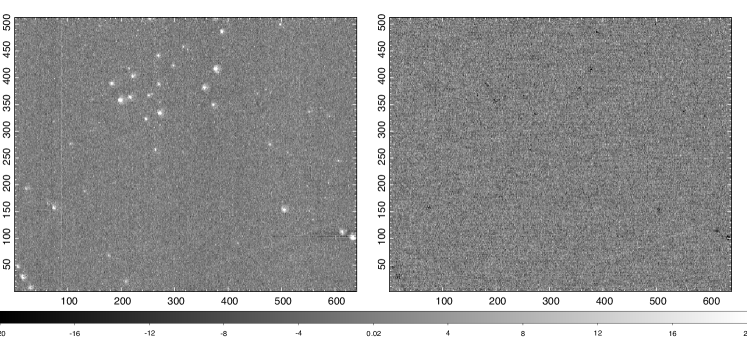
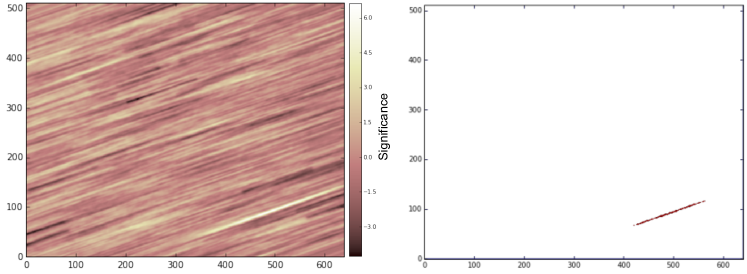
In this section we show the results of applying our maximum likelihood source detection to real data from the Space-based Telescopes for Actionable Refinement of Ephemeris (STARE) pilot survey [15, 14]. Figure 2 shows an image from this survey that we analyzed as part of our automatic detection pipeline, which is similar to that outlined in subsection 4.1. One key difference being that we used image subtraction to remove the stars, rather than masking, before running the maximum likelihood streak detection method (see the right panel of Figure 2). While no streak was originally detected in the survey, we were able to detect an ultra-faint LEO object in the lower right corner of the image with significance $\nu>5$, see Figure 3.

Fig. 2: Left: An image from the Space-based Telescopes for Actionable Refinement of Ephemeris (STARE) pilot survey [15, 14]. The ground-based survey was conducted in sidereal tracking mode thus stars appear as atmospheric PSF convolved point sources, and satellites will appear as streaks. Right: The same image after subtracting an image of the same field taken one minute earlier. Thus the majority of the stellar flux has been subtracted, however sources that move appreciably over the period of one minute (e.g. LEO’s) will remain. Operating on the differenced image enables a much higher streak detection purity, with minor completeness loss due to slightly increased noise in the differenced image (which could further be minimized by differencing a median stacked image rather than a single image). Note that the differenced image also removes static detector defects like the vertical line at the $x\sim 90$ pixel location in the left image. Both images are to the same scale.

Fig. 3: Maximum likelihood detection pipeline products for the images in Figure 2. Left: The $\nu_{\mathrm{streak}}$ with the maximum significance after running a grid based model search in $\Omega$ parameter space. A streak in the lower right of the image is detected with $>6\sigma$ significance. Right: The detected streak footprint after applying a $5\sigma$ detection threshold to the $\nu_{\mathrm{streak}}$ image.

Detecting Multiple Arbitrary Streaks in Single Image

As demonstrated in the previous sections it is relatively straightforward to detect a single streak in an image using the maximum likelihood method. However, there are often multiple streaks in a single image and these may have very different properties $\Omega$. Ideally any detection method will simultaneously find all streaks in an image, regardless of varying streak locations, lengths, and orientations, as well as deblend streaks and maintain a high purity and completeness (i.e., minimize false detections while maximizing the number of detected sources). In this section, we show that the maximum likelihood method derived in section 3 can be formally extended to enable unsupervised detection of multiple sources.

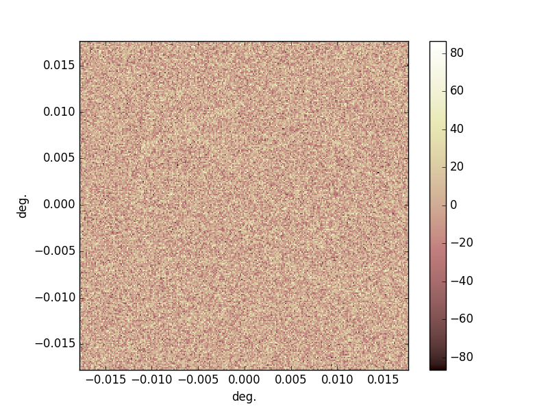
To demonstrate this capability, we simulated an image containing three streaks, Figure 4(b). As can be seen from the noise free version of the image, Figure 4(a), which is used only for presentation, two of the streaks have the exact same location parameters, $(x_{0},y_{0})$, but different orientations.

(a) Noise Free

(b) With Noise

Fig. 4: A simulated image containing three streaks convolved with a Gaussian PSF. Figure 4(a) shows the three streaks without any noise but including the PSF. Figure 4(b) is the same as Figure 4(a) but with significant random noise added such that the streak surface flux density is $<<$ than the RMS of the pixel noise.

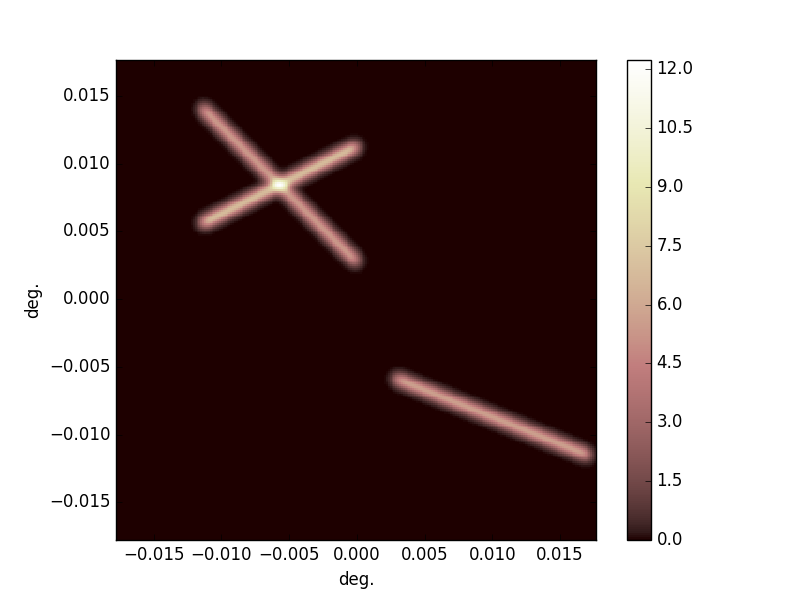
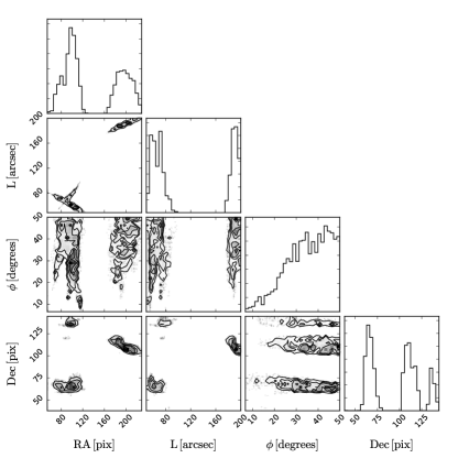
The key to detecting multiple streaks in a single image is construction of the streak model parameter $\Omega$ posterior probability densities for an entire image. This posterior probability density summarizes the probability of having sources across the range of parameter space. This posterior can be constructed by using the log likelihood, Equation 9, with a sampling method. Some examples of valid sampling methods include Markov Chain Monte Carlo (MCMC), or random/grid-based searches coupled with Sequential Importance Resampling (SIR). [12] successfully implemented an ad hoc variant of this method by performing a grid based search in $L$ and $\phi_{0}$ parameter space, using the “angle history”, and “length history” as a means of quasi-importance resampling.

For this work, we randomly sampled 10,000 points in $L$ and $\phi_{0}$ parameter space, convolving the $\Psi_{\mathrm{PSF}}$ and $\Phi+\mathrm{PSF}$ images each time with the given streak line model. Thus we had $10000\times N_{\mathrm{pixels}}$ samples. To reduce memory load we only saved samples with $\nu>5$, however this GMM method does not require such an arbitrary sample selection. Given the $\nu$ estimates associated with each sample we calculated the corresponding posterior probability and used those to resample with a SIR method. The resulting posterior is shown in Figure 5.

Fig. 5: The posterior probability density for the streak model space $\Omega$ resulting from a SIR analysis and using the likelihoods from a random search of 4(b) with the maximum likelihood detection method. To reduce memory load we only saved samples with $\nu_{\mathrm{streak}}>5$. Note that the Dec.-axis has been flipped relative to the y-axis of Figure 4.

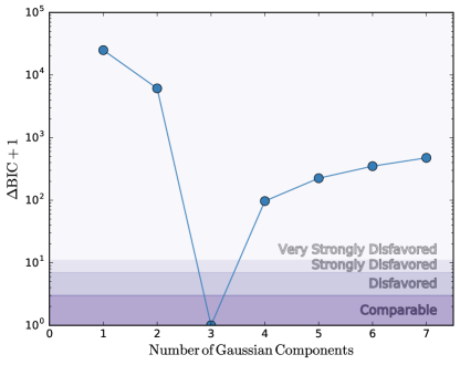
After constructing the posterior we can use this with unsupervised clustering algorithms to determine the number and properties of the streaks. In a similar fashion to the work of [2], we implement scikit- learn’s [9] GMM program and apply it to the four- dimensional posterior. We consider mixtures of 1 to 7 multivariate Gaussian components with fully unstructured covariance structures. For each number of components ($n$) we calculate the Bayesian Information Criterion (BIC) and use this to infer the optimal number of subclusters. We plot these results as,

$$\Delta\mathrm{BIC}_{n}=\mathrm{BIC}_{n}-\min\left(\mathrm{BIC}_{n}|n\in\mathbb{Z}_{1...7}\right)$$ (16)

where $\mathbb{Z}_{1...7}$ is the set of integers from 1 to 7. For convenience of interpretation we color-code regions of the $\Delta$BIC plot according to the broad model comparison categories suggested by Kass et al. [6]. From Figure 6 we see that the GMM $\Delta$BIC strongly favors the model with three streaks.

Fig. 6: A $\Delta$BIC plot comparing GMM fits to the four-dimensional streak model parameter (right ascension, declination, length, and position angle) posterior distribution from an MCMC analysis of Figure 4(b)., with varying number of Gaussian components and covariance type. The GMM analysis was done assuming a fully variable covariance type. The purple shaded regions roughly denote how a given model compares with the model that has the lowest BIC score. The best fit is a three component model, meaning that all three simulated streaks were detected and there were no false detections.

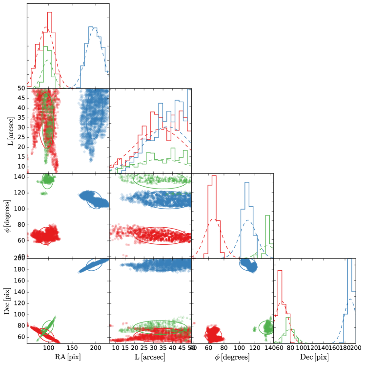
In Figure 7 we show the parameter posterior distribution but with samples color coded according to their most likely cluster membership assignment of the three-component component model. We see that while the components may overlap in some parameter spaces the fact that we can utilize all four-dimensions simultaneously we can deblend objects so long as they do not completely overlap in all parameter dimensions. Furthermore, the clustered samples provide estimates of the streak properties, including uncertainties, and can also be used as priors in subsequent forward modeling of the detected sources (see for example [13]).

Fig. 7: Four-dimensional posterior distribution of the streak model SIR fit to Figure 4(b) and their most likely cluster membership assignment for the best fit GMM (see Figure 6). For the projected one-dimensional distributions we plot the marginalized Gaussian components for the best fit model (dashed lines). For the projected two-dimensional distributions we plot projected ellipses that encompass $\sim 68\%$ of the corresponding members in the best fit model Gaussian components. The differently colored ellipses are non-overlapping in many 2D projections, which is how we are able to effectively deblend the streak images.

Summary & Discussion

Signal-matched filters have been used extensively in astronomical image detection algorithms to detect faint, low surface brightness, sources. In this conference proceeding we have outlined how signal-matched filters can be incorporated into a maximum likelihood statistical formalism. This formalism has a number of advantages. It accounts for spatially-varying source models, image noise, and PSFs. In addition, it enables easy epoch co-addition that is absent of the systemics associated with varying PSFs and the processing of data on a pixel grid.

In addition to outlining the maximum likelihood detection method we have demonstrated it on a number of simulated images, as well as an image of a real LEO object observed during the STARE proof of concept survey. We have also demonstrated how the method enables us to detect and deblend multiple ultra-faint streaks, with varying properties, in a single image.

The ability of the maximum likelihood method to recover all of the information in a given image, and combine the information from multiple epochs in a statistically rigorous manner, enables the detection of ultra-faint sources. Furthermore, the probabilistic basis of the maximum likelihood detection method enables detection of multiple objects in a given image (including blended sources), and initial estimates of the detected object properties, including uncertainties that can be consistently propagated to downstream estimates (e.g., orbit parameter estimates; see [13]). It is for these reasons that ultra-faint, low signal-to-noise, sources can still result in actionable information.

References

- [1] National Research Council. Defending Planet Earth: Near-Earth-Object Surveys and Hazard Mitigation Strategies. The National Academies Press, Washington, DC, 2010.
- [2] W. A. Dawson, M. J. Jee, A. Stroe, Y. K. Ng, N. Golovich, D. Wittman, D. Sobral, M. Brüggen, H. J. A. Röttgering, and R. J. van Weeren. MC2: Galaxy Imaging and Redshift Analysis of the Merging Cluster CIZA J2242.8+5301. ApJ, 805:143, June 2015.
- [3] G. Jogesh Babu, A. Mahabal, S. G. Djorgovski, and R. Williams. Object detection in multi-epoch data. Statistical Methodology, 5:299–306, July 2008.
- [4] N. Kaiser. Addition of Images with Varying Seeing. Technical Report PSDC-002-011-xx, Institute for Astronomy, University of Hawaii at Manoa, Honolulu, Hawaii, July 2001.
- [5] N. Kaiser. The Likelihood of Point Sources in Pixellated Images. Technical Report PSDC-002-010-xx, Institute for Astronomy, University of Hawaii at Manoa, Honolulu, Hawaii, September 2002.
- [6] Robert E. Kass and Adrian E. Raftery. Bayes factors. Journal of the American Statistical Association, 90(430):773–795, 1995.
- [7] Vladimir Kouprianov. Distinguishing features of ccd astrometry of faint geo objects. Advances in Space Research, 41(7):1029 – 1038, 2008.
- [8] Y. N. Krugly. Problems of CCD Photometry of Fast-Moving Asteroids. Solar System Research, 38:241–248, May 2004.
- [9] F. Pedregosa, G. Varoquaux, A. Gramfort, V. Michel, B. Thirion, O. Grisel, M. Blondel, P. Prettenhofer, R. Weiss, V. Dubourg, J. Vanderplas, A. Passos, D. Cournapeau, M. Brucher, M. Perrot, and E. Duchesnay. Scikit-learn: Machine learning in Python. Journal of Machine Learning Research, 12:2825–2830, 2011.
- [10] T. Schildknecht, R. Musci, M. Ploner, G. Beutler, W. Flury, J. Kuusela, J. de Leon Cruz, and L. de Fatima Dominguez Palmero. Optical observations of space debris in geo and in highly-eccentric orbits. Advances in Space Research, 34(5):901 – 911, 2004. Space Debris.
- [11] T. Schildknecht, M. Ploner, and U. Hugentobler. The search for debris in geo. Advances in Space Research, 28(9):1291 – 1299, 2001.
- [12] T. Schildknecht, K. Schild, and A. Vannanti. Streak Detection Algorithm for Space Debris Detection on Optical Images. In Advanced Maui Optical and Space Surveillance Technologies Conference, page 36, 2015.
- [13] M. D. Schneider and W. A. Dawson. Synthesis of disparate optical imaging data for space domain awareness. In Advanced Maui Optical and Space Surveillance Technologies Conference, 2016.
- [14] L. Simms, D. Phillion, W. De Vries, V. Riot, B. Bauman, and D. Carter. Orbit Refinement with the STARE Telescope. Journal of Small Satellites, 2:235–251, 2013.
- [15] L. M. Simms, W. D. Vries, V. Riot, S. S. Olivier, A. Pertica, B. J. Bauman, D. Phillion, and S. Nikolaev. Space-based telescopes for actionable refinement of ephemeris pathfinder mission. Optical Engineering, 51(1):011004–011004, January 2012.
- [16] A. S. Szalay, A. J. Connolly, and G. P. Szokoly. Simultaneous Multicolor Detection of Faint Galaxies in the Hubble Deep Field. AJ, 117:68–74, January 1999.
- [17] G. Turin. An introduction to matched filters. Information Theory, IRE Transactions on, 6(3):311–329, June 1960.
- [18] Peter Vereš, Robert Jedicke, Larry Denneau, Richard Wainscoat, Matthew J. Holman, and Hsing-Wen Lin. Improved asteroid astrometry and photometry with trail fitting. Publications of the Astronomical Society of the Pacific, 124(921):1197, 2012.
- [19] P.M. Woodward. Probability and Information Theory: With Applications to Radar. Number v. 3 in Electronics and Waves. Elsevier Science & Technology, 1953.