Synthesis of disparate optical imaging data for space domain awareness

Abstract

We present a Bayesian algorithm to combine optical imaging of unresolved objects from distinct epochs and observation platforms for orbit determination and tracking. By propagating the non-Gaussian uncertainties we are able to optimally combine imaging of arbitrary signal-to-noise ratios, allowing the integration of data from low-cost sensors. Our Bayesian approach to image characterization also allows large compression of imaging data without loss of statistical information. With a computationally efficient algorithm to combine multiple observation epochs and multiple telescopes, we show statistically optimal orbit inferences.

Introduction

The Geosynchronous Earth Orbit (GEO) is an increasingly crowded environment requiring regular monitoring for orbit determinations and refinements in catalog maintenance. When using optical telescopes to monitor GEO, many observations are needed to measure sufficient arc length to constrain an orbit. The exposure time for a single exposure is often limited by the requirement to avoid detector saturation from bright stars. Or, in the case of non-sidereal tracking, the exposure time is limited by the avoidance of star streaks covering too much detector area. The telescope aperture then limits the faintest magnitudes that can be tracked, which are correlated with satellite or debris size [6].

We present an algorithm for characterization of streaks in optical CCD imaging of arbitrary signal-to-noise ratio (assuming an initial detection has been made [3]) and subsequent orbit determinations including uncertainty propagation and combinations of information from multiple observing epochs or telescopes. We characterize streak information (position, length, and flux) via a statistical model that allows statistical compression of image information.

Method

Image forward model

We seek an analytic model for a streak image because with parameters that we can infer in a probabilistic framework. This in principle allows us to optimally utilize all the information in the streak image, including the positions, flux, and point-spread function (PSF) size. An analytic model including the PSF also avoids computing time that might be spent in numerical convolutions of the image with the PSF when rendering an image model.

We choose a Gaussian model for the PSF because the Fourier transform is also a Gaussian and the central peak of an Airy disk (the diffraction limited PSF of an unaberrated system with a circular aperture) is well approximated by a Gaussian.

$$\Pi_{i}(\mathbf{H}_{i})\equiv\exp\left(-\frac{1}{2}|\mathbf{H}_{i}|^{2}/\sigma_{\Pi}^{2}\right),$$ (1)

where $\mathbf{H}_{i}$ are angular positions in the focal plane of the $i$th telescope.

We model a streak as a product of a narrow Gaussian (representing the width that can be made arbitrarily small) and a rectangular window (representing the extent of the streak). We further assume that the streak model is evaluated in a coordinate system with the center of the streak at the origin and the extent of the streak along the $x$-axis. This can always be accomplished by means of a coordinate translation by $x_{0},y_{0}$ and a rotation by $\phi_{0}$ giving observed focal plane coordinates $\mathbf{H}$,

$$\mathbf{H}_{x} =\cos\phi_{0}(x-x_{0})-\sin\phi_{0}(y-y_{0})$$ (2)

$$\mathbf{H}_{y} =\sin\phi_{0}(x-x_{0})+\cos\phi_{0}(y-y_{0}).$$ (3)

Then (see also [9]),

$$\boldsymbol{\ell}(\mathbf{H})=\ell_{0}{\rm rect}\left(\frac{H_{x}}{L}\right)\exp\left(-\frac{1}{2}\frac{H_{y}^{2}}{\sigma_{y}^{2}}\right),$$ (4)

where $L$ is the length of the streak, $\ell_{0}$ is the surface brightness of the streak (i.e., luminosity per unit area), and ${\rm rect}$ is the rectangular window function.

The Fourier transforms of the PSF and streak model are,

$$\tilde{\Pi}_{i}(\boldsymbol{\rho})=\exp\left(-\frac{1}{2}|\boldsymbol{\rho}|^{2}\sigma_{\Pi}^{2}\right),$$ (5)

and,

$$\tilde{\boldsymbol{\ell}}(\boldsymbol{\rho})=\ell_{0}\,\rm sinc\left(\frac{L\rho_{x}}{2}\right)\exp\left(-\frac{1}{2}\rho_{y}^{2}\sigma_{y}^{2}\right).$$ (6)

The streak image after convolution with the PSF is,

$$\hat{\boldsymbol{\ell}}(\mathbf{H})=\frac{\ell_{0}}{2}\left[\rm Erf\left(\frac{L-2H_{x}}{2\sqrt{2\sigma_{\Pi}^{2}}}\right)+\rm Erf\left(\frac{L+2H_{x}}{2\sqrt{2\sigma_{\Pi}^{2}}}\right)\right]\exp\left(-\frac{1}{2}\frac{H_{y}^{2}}{\sigma_{\Pi}^{2}+\sigma_{y}^{2}}\right)\frac{\sqrt{2\pi\sigma_{y}^{2}}}{\sqrt{2\pi(\sigma_{\Pi}^{2}+\sigma_{y}^{2})}}$$ (7)

Equation 7 is our model for the image of a streak, which has parameters,

$$\omega\equiv\left[x_{0},y_{0},\phi_{0},\ell_{0},L,\sigma_{\Pi}^{2}\right].$$ (8)

We will always set $\sigma_{y}^{2}\ll\sigma_{\Pi}^{2}$ for this model.

We fit the streak image parameters $\omega$ to the pixel values of a CCD image $\mathbf{d}$ by means of a likelihood function, with the likelihood for all available images of a unique source assumed to factor into a product of the likelihoods for each image. Assuming also Gaussian, uncorrelated pixel noise in each image,

$${\rm Pr}(\mathbf{d}|\omega_{i},\sigma^{2}_{{\rm noise},i})=\prod_{i=1}^{n_{\rm telescopes}}\mathcal{N}_{\mathbf{d}_{i}}\left(\mathbf{m}(\omega_{i}),\sigma^{2}_{{\rm noise},i}\right),$$ (9)

where $\mathbf{m}$ is the model prediction for the pixel data in telescope $i$ given streak image parameters $\omega_{i}$, $\sigma^{2}_{{\rm noise},i}$ is the per-pixel noise variance in telescope $i$, and $\mathcal{N}_{x}$ indicates a Normal (or Gaussian) distribution for the variable $x$.

Given a single streak image, we infer ‘interim’ posterior constraints on the parameters of the streak image using the likelihood function in Equation 9,

$${\rm Pr}(\omega_{i}|\mathbf{d}_{i},\sigma^{2}_{{\rm noise},i})\propto{\rm Pr}(\mathbf{d}_{i}|\omega_{i},\sigma^{2}_{{\rm noise},i}){\rm Pr}(\omega_{i}|I_{0}),$$ (10)

where $I_{0}$ encodes the prior assumptions for fitting of single-epoch streak images. Sampling in the streak image parameters $\omega_{i}$ provides a convenient way to extract source information and compress the image data into a set of $K$ model parameter samples $\omega_{i;k},k=1,\dots,K$.

Preliminary orbit determination

To obtain preliminary orbit determinations (PODs), we want to sample from ${\rm Pr}(\theta|\mathbf{d})$, where $\theta$ are the orbit parameters.

The streak image parameters are

$$\omega=(x_{0},y_{0},L,\phi_{0},\ell_{0},\sigma^{2}_{\Pi})\equiv(\hat{\omega},\ell_{0},\sigma^{2}_{\Pi}),$$ (11)

where we have split out $\ell_{0},\sigma^{2}_{\Pi}$ as nuisance parameters for orbit determination.

The (osculating) Keplerian elements $\theta$ are entirely determined given the remaining streak image parameters $\hat{\omega}$ coupled with ranges, $\rho$, (i.e., line-of-sight distances) at the exposure start and end times [8],

$$\theta=\theta(\hat{\omega},\rho,t).$$ (12)

Note there is an ambiguity in the variable transformation in Equation 12 if the orbit is not known to be prograde or retrograde. In this case, both solutions must be tried. This degeneracy can be broken if subsequent exposures are taken or a time-tagging procedure as in [5] is used.

The posterior for the POD is then,

$${\rm Pr}(\theta|\mathbf{d},\alpha,t)\,d\theta\propto{\rm Pr}(\theta(\rho,\hat{\omega},t))\int d\ell_{0}d\sigma^{2}_{\Pi}\,\left[{\rm Pr}(\mathbf{d}|\omega,t){\rm Pr}(\omega|t)\right]{\rm Pr}(\rho|t,\alpha)\frac{1}{{\rm Pr}(\omega|t)}\left|\frac{d(\hat{\omega},\rho)}{d\theta}\right|\,d\theta,$$ (13)

where the bracketed expression ${\rm Pr}(\mathbf{d}|\omega,t){\rm Pr}(\omega|t)$ is the posterior from which samples of $\omega$ are drawn in the interim sampling to fit the streak image model, ${\rm Pr}(\rho|t,\alpha)$ is an asserted prior distribution for the ranges, and $\alpha$ represents the parameters describing the prior distribution. We must assert the range prior because observations of a single streak cannot constrain the range parameters.

Equation 13 suggests a sampling algorithm for POD,

1. Select $N$ (uncorrelated) samples of $\hat{\omega}_{i}$ from the interim sampling used to fit the streak image model,

2. Draw $N$ samples of $\rho_{i}$ from ${\rm Pr}(\rho|t,\alpha)$ given hyper-parameters $\alpha$ (as in [7]),

3. Compute $\theta_{i}(\rho_{i},\hat{\omega}_{i},t)$ for each $i=1,\dots,N$,

4. Optionally, re-weight or compute accept/reject sampling of $\theta_{i}$ under a new prior,

   $$p\equiv{\rm Pr}(\theta)\left|\frac{d(\hat{\omega},\rho)}{d\theta}\right|\frac{1}{{\rm Pr}(\hat{\omega}|t)}.$$ (14)

Combining preliminary orbits

After inferring PODs for each observation epoch separately, we have a set of posterior samples, $\boldsymbol{\theta}^{(i)}$, for each epoch or telescope $i$. To refine our orbit inferences, we describe a method to re-weight the samples $\boldsymbol{\theta}^{(i)}$ to propagate the information from the combination of all observations.

We use the Generalized Multiple Importance Sampling (MIS) algorithm from [4]. The MIS weights associated with the $k$th interim posterior sample $\theta^{(i)}_{k}$ are,

$$w_{k}^{(i)}\equiv\frac{\prod_{j=1}^{N_{\rm epochs}}{\rm Pr}(\mathbf{d}_{j}|\theta^{(i)}_{k})}{\sum_{j=1}^{N_{\rm epochs}}{\rm Pr}(\mathbf{d}_{j}|\theta^{(i)}_{k})},$$ (15)

where the likelihood of the single-epoch data $\mathbf{d}_{j}$ is implicitly defined by the integrand in Equation 13. The key feature to note in Equation 15 is that we evaluate the likelihood of the orbit parameters from the epoch $i$ analysis given the data from all other epochs $j$. The weights in Equation 15 are thus only large if the likelihoods of all available images are consistent with the given parameters $\boldsymbol{\theta}^{(i)}$.

To evaluate the single-epoch likelihoods in Equation 15,

1. Convert $\boldsymbol{\theta}^{(i)}_{k}$ to $\hat{\omega}^{(i)}_{k}(\boldsymbol{\theta},\mathbf{x}_{j},\boldsymbol{\gamma}_{j})$ and $\rho^{(i)}(t_{j})$ (where $\mathbf{x}_{j}$ represents the telescope position and $\boldsymbol{\gamma}_{j}$ represents the pointing vector),

2. Sample $\ell_{0},\sigma_{\Pi}^{2}$ (and, optionally, $\mathbf{x}_{j}$ and $\boldsymbol{\gamma}_{j}$) with replacement from the interim image model samples from epoch $j$,

3. Evaluate

   $${\rm Pr}(\mathbf{d}_{j}|\omega^{(i)},t_{j}){\rm Pr}(\rho^{(i)}|t_{j},\alpha)p_{j},$$ (16)

   where $p_{j}$ is defined in Equation 14.

We have also found that a kernel density approximation of ${\rm Pr}(\mathbf{d}_{j}|\theta^{(i)})$ can be sufficient for accurate evaluation of Equation 15.

Results

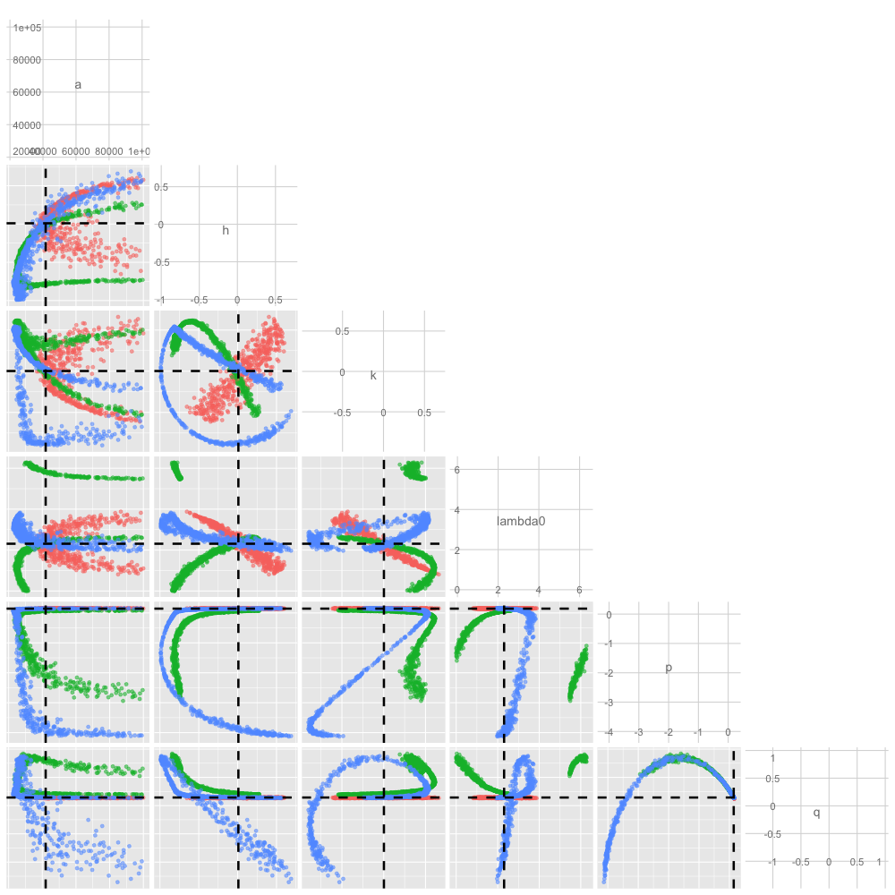
In this section we demonstrate the algorithm in section 3 with simulated images of a GEO satellite where we can compare with the known true orbit. We consider a scenario with 3 observatories at different locations: 1 telescope located on the surface of the Earth and 2 satellites in a sub-GEO orbit that are offset in orbital phase by a fraction of a period as in Figure 1 (see [2] for a related scenario).

Fig. 1: The scenario for our simulation study includes 3 telescopes observing a single GEO satellite. One telescope is ground-based and two are space-based.

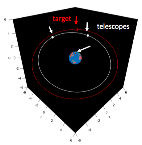
We will compare the orbit inferences from this combination of 3 telescopes to that achievable with multiple exposures taken from the single ground-based observatory. In all cases we assume 30 second exposures and pixel scales of 20 arcseconds on the ground and 10 arcseconds in space. We show the mock images in Figure 2.

Fig. 2: Mock images of a GEO satellite in a 30 second exposure taken from ground (left) and two space-based platforms (middle and right).

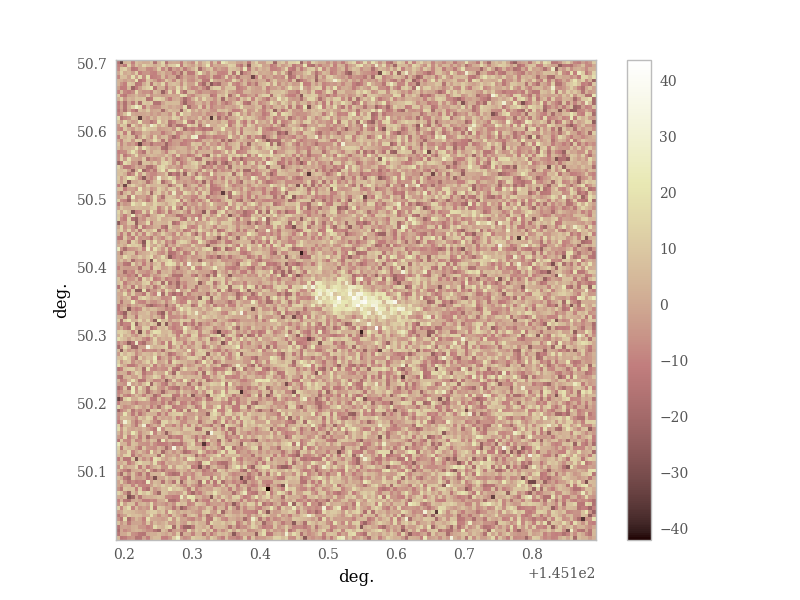
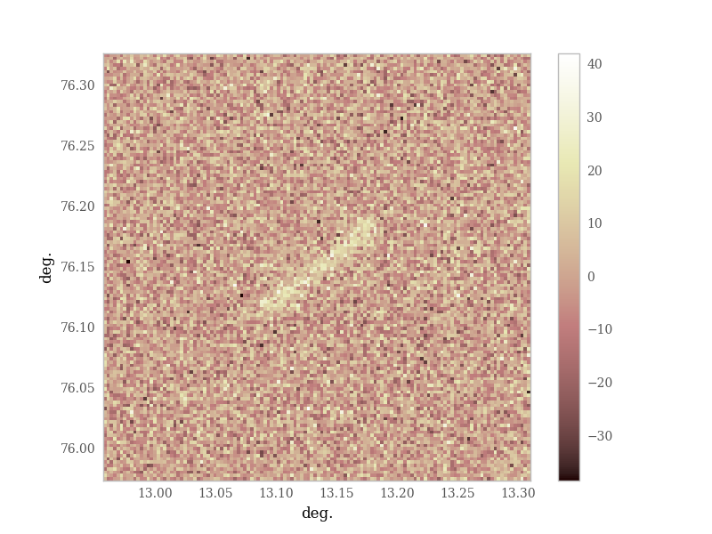
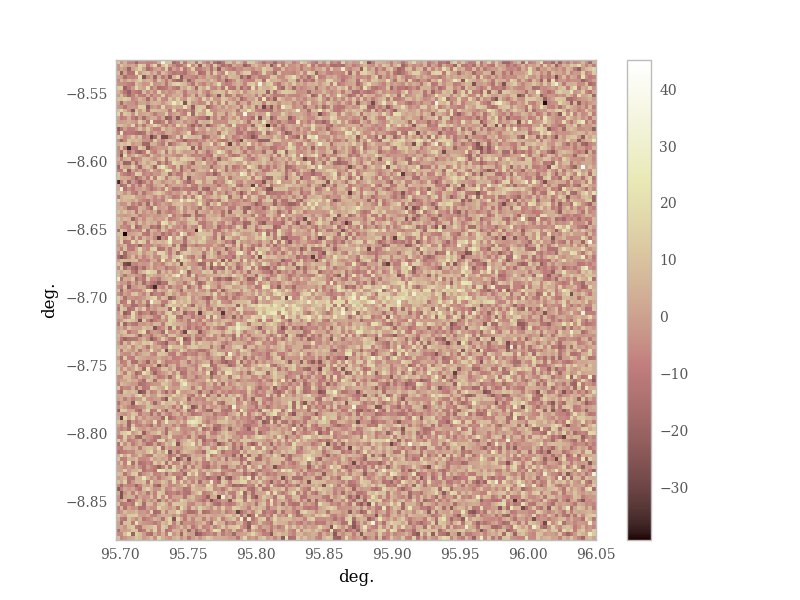
In Figure 3 we show the PODs from simultaneous observations from the ground and space telescopes as 2D marginal samples of the six equinoctial Keplerian elements [1]. Each telescope has a view of the satellite from a different location and perspective, which leads to vastly different posterior constraints on the equinoctial elements. But, while the constraints on the equinoctial elements in Figure 3 are weak and non-Gaussian for any single telescope, the regions of parameter space where the constraints from all telescopes overlap is much smaller. The geometric information from the different perspectives on a single satellite thus helps constrain the orbit.

Fig. 3: Posterior samples of equinoctial Keplerian orbital elements given a single 30-second observation of a GEO satellite as seen from telescopes either on the ground or in a sub-GEO orbit. Red: ground-based telescope. Blue/green: space-based telescopes offset in orbital phase (see text).

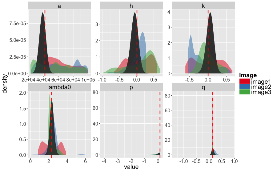
We show the 1D marginal posterior constraints on the equinoctial elements from each telescope individually and combined in Figure 4. The combined constraints shown in shaded gray use Equation 15 to re-weight the posterior samples of the orbital elements from each telescope. The shaded red, blue, and green distributions in Figure 4 show the constraints from each of the telescopes individually.

Fig. 4: The 1D marginal posterior constraints on the equinoctial Keplerian orbital elements from an observing scenario with 1 ground- and 2 space-based telescopes taking a simultaneous 30 second observation of a GEO satellite (see text). The red, blue, and green shaded distributions show the posteriors given single-telescope observations (ground or space), while the gray shaded posterior is given the combined information from all 3 telescopes.

To better understand the impact of the geometric diversity of the combined ground- and space-based observatories, we also simulate a series of consecutive 30-second exposures from the ground, separated by 5 seconds of readout time. In Figure 5 we compare the 1D marginal posterior constraints on the equinoctial elements between the consecutive ground exposures and the combined ground and space observations (using only a single simultaneous 30-second exposure on each telescope for the latter).

Fig. 5: Comparison of the marginal posterior constraints on the equinoctial elements of a GEO satellite from two observing scenarios. Green: constraints from 3 telescopes, 1 ground-based and 2 space-based taking a simultaneous 30-second observation. Red: 1 ground-based telescope taking 3 consecutive 30-second exposures. Blue: same as red, but taking 10 consecutive exposures.

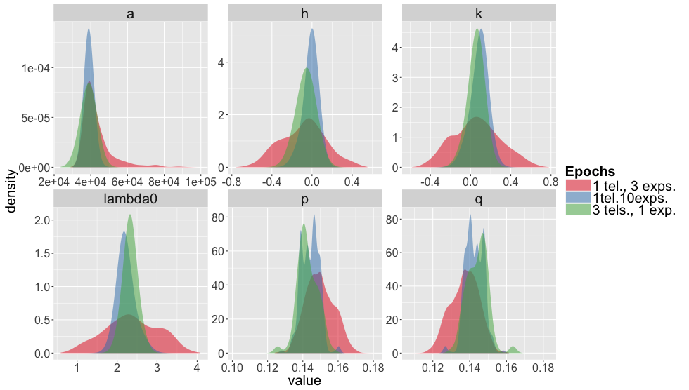
We see in Figure 5 that 3 consecutive 30-second exposures from the ground yields much more uncertain orbit inferences than the combination of 30-second exposures from the ground and space. However, 10 consecutive exposures from the ground can provide comparable orbit inferences to those from the simultaneous 30 second ground and space observations.

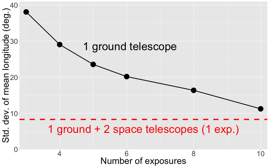
Because most of the orbit uncertainty is in the in-track direction (i.e., the timing along the orbit is most uncertain), we compare just the marginal posterior standard deviation of the mean longitudes in Figure 6. The horizontal dashed line in Figure 6 shows the standard deviation on the mean longitude inferred from the simultaneous ground- and space-based observations. The black points show the decrease in the mean longitude standard deviation with increasing numbers of consecutive 30-second exposures from the single ground-based telescope. As in Figure 5, we see that 10 exposures from the ground yields comparable constraints to the 3 telescope scenario, but that fewer consecutive exposures leaves significantly larger uncertainties on the mean longitude. That is, there is a relatively slow rate of convergence between the two observing scenarios.

Fig. 6: The marginal posterior standard deviation of the mean longitude for two observing scenarios. Red dashed horizontal line: a single simultaneous 30-second observation taken from 1 ground- and 2 space-based telescopes (see text). Black points: cumulative constraints from consecutive 30-second exposures (separated by 5-seconds readout) for a single ground-based telescope.

Conclusions

Using a simulation study, we demonstrated a new algorithm to combine images of a satellite from multiple telescopes or exposures for orbit determination and refinement.

Our algorithm uses a probabilistic forward model for satellite images in sidereal tracking optical observations. The output of a probabilistic fit to an image is samples of streak image model parameters from an interim posterior distribution. These samples constitute a form of statistical image compression. Because we propagate all uncertainties in the streak fitting process we can select images of arbitrary signal-to-noise ratio.

Given interim posterior samples of streak image parameters from an image, we perform a preliminary orbit determination (POD) using a ‘statistical ranging’ algorithm from [10, 7] to transform image positions to probabilistic samples of osculating Keplerian elements. This is a flexible approach to image processing that allows trivial parallelization of computations across distinct images.

Given the PODs from all images of a satellite (over all times and telescopes), we can combine the statistical samples of orbit parameters with a new importance sampling algorithm. The importance sampling requires new evaluations of the likelihood functions of each exposure, but can again be massively parallelized unlike Markov Chain algorithms [7].

In our simulation study we found distinct advantages in orbit determination in the combination of ground- and space-based observing deriving from the geometry of separate observatories. To perform similar orbit inferences from a single ground-based telescope requires a higher cadence of tracking observations, which we expect to become impractical as more sources and larger areas of the sky are monitored.

References

- [1] R. A. Broucke and P. J. Cefola. On the Equinoctial Orbit Elements. Celestial Mechanics, 5:303–310, May 1972.
- [2] Radu Danescu, Florin Oniga, Vlad Turcu, and Octavian Cristea. Long baseline stereovision for automatic detection and ranging of moving objects in the night sky. Sensors, 12(10):12940–12963, 2012.
- [3] W. A. Dawson, M. D. Schneider, , and C. Kamath. Blind Detection of Ultra-faint Streaks with a Maximum Likelihood Method. In Advanced Maui Optical and Space Surveillance Technologies Conference, 2016.
- [4] V. Elvira, L. Martino, D. Luengo, and M. F. Bugallo. Generalized Multiple Importance Sampling. ArXiv e-prints, November 2015.
- [5] Sun-Youp Park, Kang-Hoon Keum, Seong-Whan Lee, Ho Jin, Yung-Sik Park, Hong-Suh Yim, Jung Hyun Jo, Hong-Kyu Moon, Young-Ho Bae, Jin Choi, Young-Jun Choi, Jang-Hyun Park, and Jung-Ho Lee. Development of a Data Reduction algorithm for Optical Wide Field Patrol. Journal of Astronomy and Space Sciences, 30(3):193–206, 2013.
- [6] T. Schildknecht, R. Musci, M. Ploner, G. Beutler, W. Flury, J. Kuusela, J. de Leon Cruz, and L. de Fatima Dominguez Palmero. Optical observations of space debris in geo and in highly-eccentric orbits. Advances in Space Research, 34(5):901 – 911, 2004. Space Debris.
- [7] Michael D. Schneider. Bayesian linking of geosynchronous orbital debris tracks as seen by the Large Synoptic Survey Telescope. Advances in Space Research, 49(4):655–666, February 2012.
- [8] VA Shefer. New method of orbit determination from two position vectors based on solving Gauss’s equations. Solar System Research, 44(3):252–266, 2010.
- [9] Peter Vereš, Robert Jedicke, Larry Denneau, Richard Wainscoat, Matthew J. Holman, and Hsing-Wen Lin. Improved asteroid astrometry and photometry with trail fitting. Publications of the Astronomical Society of the Pacific, 124(921):1197, 2012.
- [10] J. Virtanen, K. Muinonen, and E. Bowell. Statistical ranging of asteroid orbits. Icarus, 154(2):412–431, 2001.