MULTIVARIATE GARCH WITH DYNAMIC BETA

Abstract

We investigate a solution for the problems related to the application of multivariate GARCH models to markets with a large number of stocks by restricting the form of the conditional covariance matrix. The model is a factor model and uses only six free GARCH parameters. One factor can be interpreted as the market component, the remaining factors are equal. This allow the analytical calculation of the inverse covariance matrix. The time-dependence of the factors enables the determination of dynamical beta coefficients. We compare the results from our model with the results of other GARCH models for the daily returns from the S&P500 market and find that they are competitive. As applications we use the daily values of beta coefficients to confirm a transition of the market in 2006. Furthermore we discuss the relationship of our model with the leverage effect.

1 Introduction

The estimation of co-movement between stocks is an essential problem in the analysis of asset returns, financial integration, and for portfolio management. On the one side, the statistical properties of asset returns necessitate to treat them in a setting that includes time-varying volatility. The most common setting thus are GARCH models. In many analysis of co-movement one would however also like to analyze samples that cover entire markets and which can thus be very large. This is at odds with many multivariate versions of GARCH models.

A multivariate GARCH model for $N$ stocks can be characterized by the dynamics of the conditional covariance matrix $H(t)$ and by its mean $\bar{H}$. The number of so-called nuisance parameters in $\bar{H}$ typically exceeds the power of a maximum likelihood estimate (MLE) for samples like the constituents of the S&P index. A possible solution are methods using covariance targeting (Engle and Mezrich, 1996) that replace $\bar{H}$ by the observed time-averaged covariance $C$. Since $C$ has similarity with a random matrix one can expect the uncertainty in $\bar{H}$ to be in the order of $\sqrt{N/T}$ (see Laloux et al., 1999; Marčenko and Pastur, 1967). A different solution are shrinkage methods as proposed by Engle et al. (2018) which renders improved estimates of the eigenvalues of $\bar{H}$ but not its eigenvectors.

We will overcome the problem of estimating $\bar{H}$ in large samples by a restricted form of $\bar{H}$ as in the $K$-factor model (see Bauwens et al., 2006). In this method only parts of $C$ are used that can be determined with a relative accuracy in the order of $\sqrt{1/T}$.

Another issue for estimations are the GARCH parameters that govern the dynamics of $H(t)$. In the VEC model (Bollerslev et al., 1988) the elements of $H(t)$ are treated as a $N(N+1)/2$ vector, which can lead to a large number of parameters. In its scalar version (Ding and Engle, 2001) only two parameters remain. The $K$-factor BEKK model (Engle and Kroner, 1995) uses $N$-dimensional matrix multiplication. Also in this model the number of parameters can become very large unless one uses the scalar version with a manageable number of $2K$ parameters.

Last but not least use of MLE requires the estimation of $H^{-1}(t)$ when Gaussian noise is used, and even worse $H^{-1/2}(t)$ for general noise. For large $N$ numerical inversion can be prohibitive. In $K$-factor models these time consuming calculations can be done outside MLE resulting in $K$ independent univariate GARCH models for the factors. A restricted form for $H(t)$ has also been proposed in the DECO model (Engle and Kelly, 2012) which assumes the same time-dependent correlation between all pairs of stocks and therefore also circumvents these issues.

Our model is loosely based on the BEKK model and adds two effective dynamic factors. We define one common volatility factor $v_{0}(t)$ and $N-1$ degenerate equal factors $v_{1}(t)$. This ensures the existence of $H^{-1}(t)$ and at the same time allows its analytical calculation. As the second part we use a rotation of the eigenvector that belongs to the $v_{0}(t)$ factor. In contrast to the GO-GARCH model (van der Weide, 2002) this rotation is time-dependent and is determined dynamically. This part of the model therefore delivers time-dependent beta coefficients relative to the market in the spirit of a CAPM.

Summarized, the model dynamics lead to a coupled system of GARCH recursions for the factors $v_{k}(t)$ and a vector recursion for $\beta(t)$. Only six GARCH parameters have to be estimated by MLE.

The paper is organized in the following way. The definition of our model and the derivation of the recursion are described in section 2 together with a comparison to other models. We apply the estimation by MLE to the daily returns of 356 stocks from the S&P market in the years 1995-2013 in section 3. We then compare the estimation results with other models in section 4. Section 5 contains two applications. By using our $\beta(t)$ we verify a transitions in the market observed by Raddant and Wagner (2017). As a second application we investigate the correlation of the leverage effect with $\beta$. The last section contains some conclusions.

2 Multivariate GARCH with restricted covariance

2.1 Model for the covariance matrix

We consider a time series of returns for $N$ stocks with length $T$ denoted by $r_{i}(t)$ with $i=1\dots N$ and $t=1\dots T$. We assume the mean of $r_{i}(t)$ with respect to $t$ is zero. In a multivariate GARCH model $r(t)$ are related to a noise $\varepsilon(t)$ by

$$r(t)={H(t)}^{1/2}\;\varepsilon(t)$$ (1)

The i.i.d. $\varepsilon$ have mean zero and variance one. The matrix $H(t)$ corresponds to the conditional covariance of $r_{i}(t)$. The dynamics of $H(t)$ are expressed by a recursion formula that relates $H(t+1)$ to the values of $H(t)$ and the returns at time $t$. A well-known example for such a model is the $K$-component BEKK(1,1,K) model (Engle and Kroner, 1995) in which the recursion is normally stated like this

$$H(t+1)=\Omega+\sum_{k}A_{k}\bigl{(}r(t)r(t)^{\prime}\bigr{)}A_{k}^{\prime}+B_{k}H(t)B^{\prime}_{k}$$ (2)

The model that we are going to introduce is different from the BEKK model, however, the structural form of the recursion for $H(t)$ has some similarities. As a starting point, consider the following specification

$$H(t+1)=H(t)+\sum_{k=0}^{K-1}\bigl{[}A_{k}\bigl{(}r(t)r(t)^{\prime}-H(t)\bigr{)}A_{k}+G_{k}\bigl{(}\bar{H}-H(t)\bigr{)}G_{k}\bigr{]}$$ (3)

where $A_{k}$ and $G_{k}$ are time-independent symmetric $N\times N$ matrices. $\bar{H}$ denotes the expected value of $H(t)$.

There are several important differences in this equation compared to other GARCH models. In many applications of multivariate GARCH models a recursion like equation (3) applies to the standardized returns and the correlation matrix $R$. In our case it applies to the conditional covariance matrix $H(t)$. This means that we preserve the information on the level of $r$, which will help to define $\beta$-values. The recursion also exhibits clearly the fixed point $H(t)=\bar{H}\;$ if $\;r(t)r(t)^{\prime}$ is replaced by its conditional expected value. The parameters in $A_{k}$ describe how fast $H(t)$ returns to its mean $\bar{H}$ after a disturbance by $r(t)r(t)^{\prime}$, $G_{k}$ describes the persistence of $H_{t}$ (similar yet not identical to $B$ in other GARCH models). This specific form of (3) will be helpful in the following generalization for time-dependent $A_{k},G_{k}$.

The linearity of equation (3) also allows the evaluation with linear algebra. We can use this property by using the following representation of symmetric matrices $M$ with dimension $N$

$$M=\sum_{k=0}^{K-1}\;\lambda_{k}\;P_{k}$$ (4)

with $N\times N$ projection matrices $P_{k}$ satisfying the orthogonality relations

$$P_{k}\cdot P_{l}=P_{k}\;\delta_{lk}$$ (5)

and the completeness relation with the unit matrix $I$

$$\sum_{k=0}^{K-1}\;P_{k}=I$$ (6)

It is important to note that the sums in equations (4) and (6) run only over the different eigenvalues $\lambda_{k}$. The trace of $P_{k}$ gives the multiplicity of $\lambda_{k}$. In the non-degenerate case ($K=N$) the $P_{k}$ are the dyadic products of the eigenvectors. For $K<N$   $P_{k}$ are independent of the particular choice of the eigenvectors. Functions of $M$ as for $H(t)$ in equation (3) can be calculated with

$$f(M)=\sum_{k=0}^{K-1}\;f(\lambda_{k})\;P_{k}$$ (7)

This formalism is particular useful in the case of a single eigenvalue $\lambda_{0}$ and $N-1$ degenerate eigenvalues $\lambda_{1}$ ($K=2$). From equation (6) we see that essentially only one projector $P_{0}$ exists with $P_{1}=I-P_{0}$.

The eigenvalue-spectrum of the covariance matrix is related to the projection matrices by

$$C=\frac{1}{T}\sum_{t=1}^{T}\;r(t)r^{\prime}(t)=\sum_{k=0}^{N-1}\;\lambda_{k}\;P_{k}$$ (8)

In figure 1 we show the eigenvalue spectrum for the S&P data ($\mbox{N=356},\mbox{T=4782}$). $C$ exhibits one large eigenvalue $\lambda_{0}$ and $N-1$ eigenvalues of order $\lambda_{0}/N$. Within the framework of a multivariate GARCH model one can interpret this behavior as if the true covariance matrix $E[H]$ had a single eigenvalue $\lambda_{0}$ and $N-1$ degenerate eigenvalues. The noise transforms them into a MP spectrum as described by Marčenko and Pastur (1967), which qualitatively agrees with the observed spectrum of $C$.

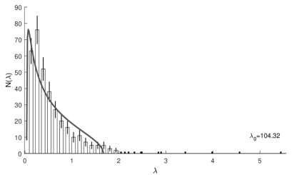
Figure 1: Histogram of eigenvalue spectrum of the covariance matrix $C$ for the daily returns of 356 S&P constituents. Returns are normalized to have $trace(C)=N$. The largest eigenvalue $\lambda_{0}=104$ is not shown. The curve corresponds to a MP spectrum. See appendix D for information on the calculation of the errors.

To arrive at a new form of $H(t)$ we assume a two component structure as in $C$ at each $t$ and write $H(t)$ as

$$H(t)=N\;v_{0}(t)\;P_{0}(t)\;+v_{1}(t)(I-\;P_{0}(t))$$ (9)

with the projector $P_{0}(t)$

$$P_{0}(t)=\frac{1}{N}\beta(t)\beta^{\prime}(t)$$ (10)

in terms of the eigenvector $\beta$, which is normalized to $\beta^{\prime}(t)\cdot\beta(t)=N$.

The form assumed in equation (9) actually corresponds to a $K=N$ factor model. The factors are the eigenvalues of $H(t)$. The first factor is $Nv_{0}(t)$. This component of the large eigenvalue of $C$ can be regarded as the market (see, e.g., Laloux et al., 1999) and therefore the first part in equation (9) can be interpreted as a time-dependent market factor. When we project $r(t)$ on the eigenvector $\beta(t)$ we obtain a market return $r_{M}(t)$

$$r_{M}(t)=\frac{1}{N}\beta^{\prime}(t)r(t)$$ (11)

Due to the relation

$$\beta_{i}(t)=\frac{E_{t-1}[r_{i}(t)r_{M}(t)]}{E_{t-1}[r_{M}^{2}(t)]}$$ (12)

$\beta_{i}(t)$ can be interpreted similar to beta coefficients in a CAPM approach (Sharpe, 1964; Lintner, 1965) relative to $r_{M}(t)$. A similar definition for conditional betas can be found in Engle (2016). Additionally we have $N-1$ degenerate factors $v_{1}(t)$ which together form the second component and show as the second term in equation (9).

We can now apply this two component structure and modify the recursion into a factor model (see Lin, 1992) with time-dependent $A_{k}$ and $G_{k}$ with

$$A_{k}(t)=\sqrt{\alpha_{k}}\;P_{k}(t)\quad\mbox{and}\quad G_{k}(t)=\sqrt{\gamma_{k}}\;P_{k}(t)$$ (13)

In order to make also the $\beta$ in the recursion dynamic we have to add the off-diagonal terms that allow for a transition between $P_{0}(t)$ and $P_{1}(t)$. These terms contribute only to $r(t)r(t)^{\prime}$ and $\bar{H}$. After adding those terms our recursion reads

$$H(t+1)=H(t) +\sum_{k=0,1}P_{k}(t)\left[\alpha_{k}\left(r(t)r^{\prime}(t)-H(t)\right)+\gamma_{k}\left(\bar{H}-H(t)\right)\right]P_{k}(t)$$

$$+P_{0}(t)\left[\alpha_{01}r(t)r^{\prime}(t)+\gamma_{01}\bar{H}\right]P_{1}(t)$$

$$+P_{1}(t)\left[\alpha_{01}r(t)r^{\prime}(t)+\gamma_{01}\bar{H}\right]P_{0}(t)$$ (14)

The six parameters of our model can be estimated by maximum likelihood, for details see appendix B.

For the mean value $\bar{H}$ we assume the same restriction as for $H(t)$

$$\bar{H}=\bar{v}_{0}\;\bar{\beta}\bar{\beta}^{\prime}+\bar{v}_{1}(I-\frac{\bar{\beta}\bar{\beta}^{\prime}}{N})$$ (15)

Details on covariance targeting and the expected error are described in detail in appendix C. We can determine the parameters $\bar{v}_{0,1}$ and $\bar{\beta}$ from the observed covariance matrix $C$ with relative accuracy $\frac{1}{\sqrt{T}}$ under the assumption of slowly varying $v_{0}(t)$ and $\beta(t)$.

The recursion for $H(t+1)$ is obviously tied to the recursions for $v_{0,1}(t+1)$ and $\beta(t+1)$. By performing the operation $tr\;P_{k}(t)(\cdot)\;$ on both sides of equation (2.1) one obtains two equations for $v_{k}(t+1)$. If we apply both sides of equation (2.1) on $\beta_{i}(t)$ we find a vector $D_{i}(t)$ which determines the change of $\beta(t+1)$:

$$D_{i}(t)=\alpha_{01}\;r_{M}(t)\big{(}r_{i}(t)-r_{M}(t)\beta_{i}(t)\big{)}+\gamma_{01}\bar{m}(t)\bar{v}_{0}\big{(}\bar{\beta}_{i}-\bar{m}(t)\beta_{i}(t)\big{)}$$ (16)

The details are given in appendix A. Since the results look rather complicated, we quote them here only in the limit $N\gg 1$. In the application to the S&P market we found no difference in using the full solution from appendix A. The recursion for $v_{0}(t+1)$ is given by

$$m^{2}(t)v_{0}(t+1)=R_{0}(t)$$ (17)

with $R_{0}(t)$ denoting the operation $tr\;P_{0}(t)(\cdot)$ on the r.h.s. of equation (2.1)

$$R_{0}(t)=v_{0}(t)+\gamma_{0}\big{(}\bar{m}^{2}(t)\bar{v}_{0}-v_{0}(t)\big{)}+\alpha_{0}\left(r_{M}^{2}(t)-v_{0}(t)\right)$$ (18)

Equation (17) depends on the angle $\phi(t)$ between $\beta(t+1)$ and $\beta(t)$ given by the overlap $\cos(\phi(t))={m}(t)=\beta^{\prime}(t+1)\cdot\beta(t)/N$. Similarly, $\bar{m}(t)=\bar{\beta}^{\prime}\cdot\beta(t)/N$ corresponds to the angle between $\beta(t)$ and $\bar{\beta}$. The overlap ${m}(t)$ is determined from the normalization condition $\beta^{\prime}(t+1)\cdot\beta(t+1)=N$ with

$$m^{2}(t)=\left[1+\frac{D^{\prime}(t)\cdot D(t)}{N\;R_{0}^{2}(t)}\right]^{-1}$$ (19)

The recursion for $\beta(t+1)$ is expressed in terms of $D(t)$ by

$$\beta_{i}(t+1)={m}(t)\left[\beta_{i}(t)+\frac{D_{i}(t)}{R_{0}(t)}\right]$$ (20)

$\beta_{i}(t+1)$ can change only for deviations of $r(t)$ from the market return $r_{M}(t)$ and deviations of $\beta(t)$ from the mean value $\bar{\beta}$. Since $D^{\prime}(t)\cdot D(t)\propto N$ there is no $N$-dependence in equation (19). When $v_{0}(t+1)$ is known we can obtain the recursion for $v_{1}(t+1)$:

$$v_{1}(t+1)= \;v_{1}(t)-(1-m^{2}(t))v_{0}(t+1)+\alpha_{1}\bigl{(}\frac{r^{2}(t)}{N}-r_{M}^{2}(t)-v_{1}(t)\bigr{)}$$

$$+\gamma_{1}(\bar{v}_{1}+(1-\bar{m}^{2}(t))\bar{v}_{0}-v_{1}(t))$$ (21)

The returns $r(t)$ appear in the recursions (17) through the market component $r_{M}(t)$ and in (16) and (2.1) through the component perpendicular to $\beta(t)$. The recursions differ from those in factor models with constant eigenvectors of $H$ in the interpretation of $\bar{v}_{k}$ and $\bar{\beta}$. They are determined by covariance targeting from the empirical covariance matrix $C$ (see appendix C). Due to the non-linearity of the recursions they may differ from the expectation values of $v_{k}(t)$, resp. $\beta(t)$. For small $\alpha_{01}$ the recursions have a fixed point solution $v_{k}(t)=\bar{v}_{k}$ and $\beta(t)=\bar{\beta}$. A necessary condition for its stability are the following inequalities for the GARCH parameters $\alpha_{k}$ and $\gamma_{k}$

$$0<\gamma_{k}<\gamma_{k}+\alpha_{k}<1$$ (22)

2.2 Relation to other models

One class of multivariate GARCH models suitable for large $N$ are factor models. They are characterized by using constant $P_{k}$ with rank 1 obtained from $C$ by equation (8) with the $K$ largest eigenvalues. A model structure similar to O-GARCH (Alexander, 2001) could be achieved by setting $A_{k}=\sqrt{\alpha_{k}}P_{k}$ and $G_{k}=\sqrt{\gamma_{k}}P_{k}$ with time-dependent $\lambda_{k}(t)$ in $H(t)=\sum\lambda_{k}(t)P_{k}$. A slightly more complex approach are full-factor models like Vrontos et al. (2003) where the conditional correlations obey a GARCH behavior, a feature which has some similarity with the behavior of our dynamic $\beta$.

Another model is the GO-GARCH (van der Weide, 2002), which is applied to the de-correlated returns $\tilde{r}(t)=C^{-1/2}\;r(t)$. The $K$ principal components of $\tilde{r}$ are rotated by a $K-$dimensional rotation. The additional $K(K-1)/2$ angles are additional parameters in MLE. Our model therefore may be called an effective two-factor model. It differs from these factor models by two features. The first is that we have always two factors. The factor $v_{0}(t)$ describes the market and we can interpret the nonmarket component $v_{1}(t)$ as a second factor that corresponds to $N-1$ identical factors $v_{1}(t)$. Second, we use a time-dependent $P_{k}(t)$. Equation (20) (or equation (40) in appendix A) corresponds to a time-dependent rotation with angle $\cos(\phi(t))=m(t)$ as in a $K=2$ GO-GARCH. However, $\phi(t)$ is determined by the recursion and not by estimation.

For the large literature on other factor ARCH, GARCH and DCC models the reader is referred to Bollerslev et al. (1992) and Zhang and Chan (2009).

Another class of models avoids numerical calculation of $H^{-1}(t)$ by a restricted $H(t)$ as in our model. An example is the DECO model of Engle and Kelly (2012). In the conditional correlation matrix $R(t)$ pairwise correlations are equal

$$R(t)=(1-\rho(t))\;I\;+\;\rho(t)$$ (23)

which allows analytical calculation of $R^{-1}(t)$. In this model first the diagonal matrix of conditional expectation values $D_{i}^{2}(t)$ of $r_{i}^{2}(t)$ is determined by $N$ univariate GARCH models. With this one can then calculate $H(t)=D(t)R(t)D(t)$ and obtain the average correlation $\rho(t)$ from the DCC recursion. Our model could reproduce a DECO type model by setting $\beta(t)=1$ with

$$\rho(t)=\left(1+\frac{v_{1}(t)}{v_{0}(t)}\right)^{-1}$$ (24)

3 Estimation and results for S&P stocks

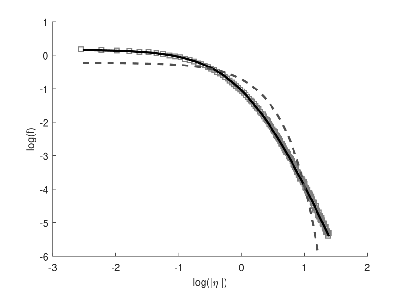
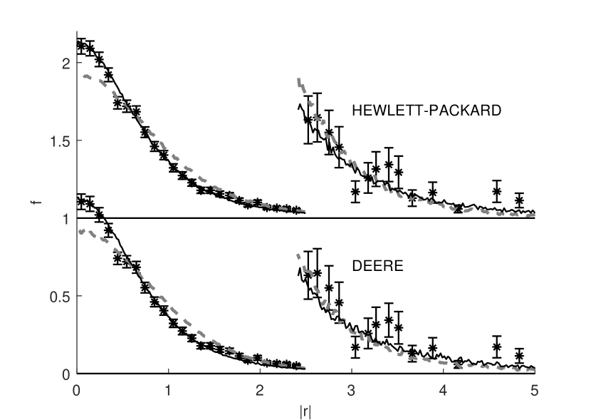
Figure 2: The left panel shows the pdf of all GARCH filtered returns $\eta_{G}(t)_{i}$ obtained from the raw returns by applying (25). The black line corresponds to a fitted t-distribution with $\nu=3.32$, the broken gray line shows a Gaussian distribution. In the right panel two typical pdfs for stocks of the S&P market are compared with the predicted pdf using t-distributed (black) or Gaussian (gray) noise (see appendix D for calculation of errors). The values (log of the pdf) $|r|>2.5$ are multiplied by a factor of 10. The theoretical curves are based on the 2-parameter fits as shown in table 1.

3.1 Preliminary fit and noise dependence

In this section we describe the maximum likelihood estimation with data of daily returns of 356 stocks that were constituents of the S&P index for the years 1995-2013. For our analysis we use data from Thompson Reuters on the closing price of stocks which were continuously traded with sufficient volume throughout the sample period and had a meaningful market capitalization.

The scale of returns is arbitrary. We choose to normalize $r(t)$ such that the average of $r_{i}^{2}(t)$ over all $i$ and $t$ is equal to one. This affects the scale in figures 2, 4, 6, 8 and 12.

$N_{par}$	$L/T$	$\alpha_{0}\cdot 10^{2}$	$\gamma_{0}\cdot 10^{2}$	$\alpha_{1}\cdot 10^{1}$	$\gamma_{1}\cdot 10^{2}$	$\alpha_{01}\cdot 10^{2}$	$\gamma_{01}\cdot 10^{2}$
2	-52.2	4.871	0.383	$\alpha_{0}$	$\gamma_{0}$	$\alpha_{0}$	$\gamma_{0}$
		(0.068)	(0.014)
2	-2.57	3.132	0.284	$\alpha_{0}$	$\gamma_{0}$	$\alpha_{0}$	$\gamma_{0}$
		(0.048)	(0.011)
4	-0.10	1.592	0.328	2.472	0.766	$\alpha_{0}$	$\gamma_{0}$
		(0.042)	(0.016)	(0.050)	(0.078)
6	0.00	5.14	4.13	2.487	0.781	1.673	0.298
		(0.16)	(0.31)	(0.041)	(0.065)	(0.044)	(0.014)

Table 1: Maximum likelihood estimates of the parameters for the S&P market. Column one states the number of parameters, column two the values of the log likelihood per time relative to the six parameter fit. Standard errors are given in parentheses. The results in the two top rows are obtained with Gaussian noise, in rows 3-8 with t-distributed noise.

We calculate the log likelihood $L$ of our model with the exact solution of the recursion as described in appendix A. The initial values $\bar{v}_{\nu}$ and $\bar{\beta}$ have been determined from the observed covariance matrix $C$ in the first 4 years. In a preliminary fit we use only two parameters with $\alpha_{1}=\alpha_{0}$, $\alpha_{01}=\alpha_{0}$, $\gamma_{1}=\gamma_{0}$ and $\gamma_{01}=\gamma_{0}$ together with a Gaussian distributed noise. The resulting log likelihood (divided by $T$) and the parameter values are given in table 1.

As a check on the property of this fit we consider the so-called de-garched returns $\eta_{G}(t)$. These are obtained by inverting equation (1)

$$\eta_{G}(t)=H(t)^{-1/2}\;r(t)$$ (25)

If the GARCH model represents the data exactly $\eta_{G}(t)$ should be again Gaussian distributed. This is not the case, as the pdf in the left panel of figure 2 shows. The pdf for $\eta_{G}(t)$ is well described by a Student’s t-distribution with a tail index of $\nu=3.32$. This motivates to repeat the estimate with a t-distributed noise. The estimated value of $\nu=3.25$ agrees within the errors with the value obtained before (see figure 2). The resulting $L$ ($2^{nd}$ column in table 1) corresponds to an astronomical increase of probability. Even the pessimistic evaluation using the probability change per $t$ given by $exp(-\Delta L/T)$ is highly significant.

Such a strong noise dependence is not present in applications of univariate GARCH(1,1) models. There, the tail index can be reproduced either by t-distributed or Gaussian noise. However, since our model (hereafter called RMG for restricted matrix GARCH) has only four GARCH parameters, $\alpha_{0,1}$ and $\gamma_{0,1}$, the tail cannot be matched for all $N$ stocks when Gaussian noise is used (see also Wagner et al., 2010, for a non-parametric moment analysis of stocks and indices).

In the right panel of figure 2 two typical pdfs of returns are compared with the predicted density either using t-distributed (black line) or Gaussian (broken gray line) noise. The latter describes the tails but fails grossly for the Gaussian region near $r=0$ and in the transition to the tail. Therefore, in all subsequent estimations we use a t-distributed noise with $\nu=3.35$.

3.2 Using simulated returns to evaluate the fit

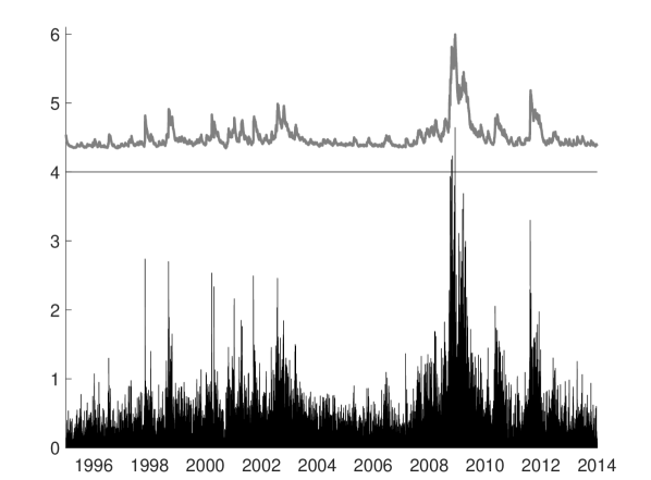
Figure 3: Market factor $\sqrt{v_{0}(t)}$ (top) and market return $|r_{M(t)}|$ (bottom). A value of 2 is added to $\sqrt{v_{0}(t)}$

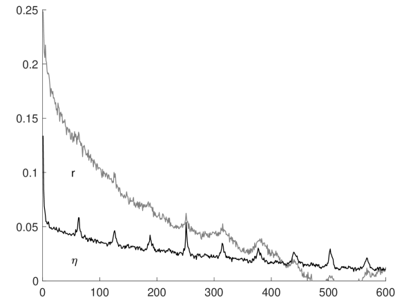
Figure 4: Autocorrelation for returns $|r_{i}(t)|$ averaged over all stocks (top) and the averaged GARCH filtered returns $|\eta_{G}(ti)|$ (bottom).

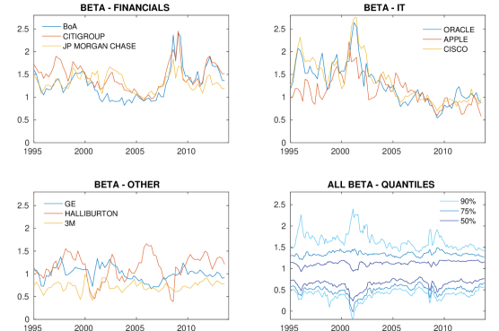
Figure 5: Beta values from the RMG model. The top panels and the bottom left panel show beta values for different stocks, averaged over a 60-day window. The bottom right panel shows the dynamics of the distribution of beta values by the quantiles, using a 20-day window.

To make sure that our model describes the distribution of returns adequately we chose to simulate the returns and to compare them to the empirical ones.

Equation (1) predicts $r(t)$ for given $H(t)$ from any GARCH model and noise at time $t$. This relationship can easily be utilized for a Monte Carlo simulation. By multiplying $H(t)^{-1/2}$ with a vector of noise we obtain simulated predicted returns $\hat{r}(t)$. When we repeat this process with different noise $n_{sim}$ times we obtain a range of possible values for the returns. By performing this procedure at all $t$ we obtain $n_{sim}T$ predictions for $\hat{r}$. Individual time series cannot be obtained, however, average values as pdf should agree with the observed quantities.

As we will see in section 4, this procedure can also be used to compare distributions of covariances for different models. To obtain smooth distributions we found that $n_{sim}=10$ is sufficient for the pdf of $\hat{r}$, covariances require $n_{sim}=40$).

The drawback of the preliminary two parameter fit consists in the small value for $\gamma_{0}$. The estimate corresponds to autocorrelation that lasts for 339 days, which is roughly twice as long as we would expect from the observed individual $|r_{i}(t)|$. The likelihood improves when we add $\alpha_{01}=\alpha_{0}$ and $\gamma_{01}=\gamma_{0}$ to the estimation (third row in table 1). However, only after including all six $\alpha$ and $\gamma$ parameters the likelihood increases again and we obtain a reasonable value for $\gamma_{0}$. The estimates for the parameters that govern the dynamics of $\beta$ are smaller by comparison, indicating that $\beta(t)$ varies much less than the factors $\sqrt{v_{\nu}(t)}$. As in any GARCH model, these exhibit much less fluctuations than the underlying returns. This is shown in figure 4 where the market factor $\sqrt{v_{0}(t)}$ is compared with $r_{M}(t)$.

More details on the autocorrelation are shown in figure 4, where we compare the GARCH filtered returns $|\eta_{G}(t)_{i}|$ with $|r_{i}(t)|$ averaged over all stocks $i$. The large statistics allow to resolve the peaks at multiples of three months, which are caused by the dividend pay days. These correlations are outside of the realm of any GARCH and survive the filtering. One can however see that the autocorrelation in $\eta$ is not perfectly removed. The reason is that with just 6 parameters the model gets the volatility right on average but mutes (inflates) stocks with very high (low) volatility since the $\beta$ move slower than $v_{0}$. As we will see in section 4.2, this particular weakness however does not carry over to the estimated covariances.

3.3 Beta values for financials and IT companies

Figure 5 finally gives an overview about the beta values that can be obtained from the RMG. Note that these betas are normalized to $\beta^{\prime}(t)\cdot\beta(t)=N$. The top left panel shows the development of beta values for some financial stocks, the top right shows the beta of IT-related companies. Stocks from both groups show strong similarity within their group. The bottom left panel shows the beta for stocks from other sectors. They develop much more diverse. The bottom right panel illustrates how the distribution of beta values has develops over time. At the times of the IT bubble and the Lehmann crisis we observe peaks for the beta values but also a much wider distribution in general.

4 Comparison with other GARCH models

In the following we will compare the estimation results of our model with those of other multivariate GARCH models. We will look at the predicted returns and covariances. Here we are interested in the practical implications of the dynamics of the model for application. In particular we are interested in a rough approximation of the precision of the estimated covariances with respect to the empirical data. A formal model comparison and selection process would be outside the scope of this paper.

4.1 Comparison of distributions of returns

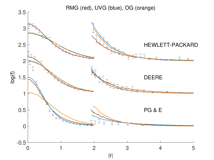
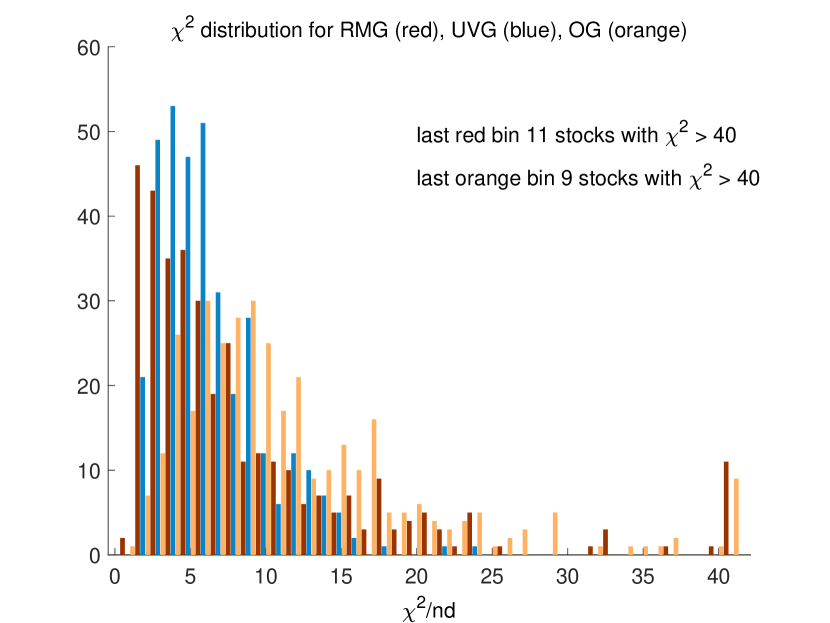
Figure 6: The left panel shows the pdf of returns compared with the prediction of RMG (red), UVG (blue) and OG (orange). The right panel shows a histogram of $\chi^{2}$ for all stocks for RMG, UVG and OG.

We start by comparing the predicted pdf of stock returns from the RMG model discussed in section 3 with those of the univariate GARCH(1,1) (abbreviated UVG) and OGARCH model (hereafter abbreviated OG). In both cases we use i.i.d. Gaussian $\varepsilon$ for the noise.

The left part of figure 6 shows that the pdf for the same two stocks as in figure 2 is in reasonable agreement with the three models. RMG and OG fail in cases where the leading eigenvector does not dominate $H(t)$, as the third example for PG&E shows.

For a more comprehensive comparison we use the $\chi^{2}/n_{d}$ ratio, which is the sum of quadratic deviation in units of the squared error divided by the number $n_{d}$ of bins. A histogram that shows how well the distributions of predicted returns fit the data measured by these ratios for all 356 stocks of the S&P market is shown for RMG, OG and UVG in the right panel of figure 6. All three distributions exhibit a peak around a value of 4-5 which corresponds to the 5% confidence level. Values between 10-20 lead still to a qualitative description (see appendix D for details on the calculation of the statistics). In contrast to UVG, both RMG and OG have a small fraction (5%) of outliers mainly from the energy sector as PG&E. On average RMG performs better than OG which may be due to the systematic error by covariance targeting. We stress that for UVG and OG 712 parameter have to be determined. The only six parameters used in RMG lead to a much more parsimonious description of the data.

4.2 Comparison of covariances

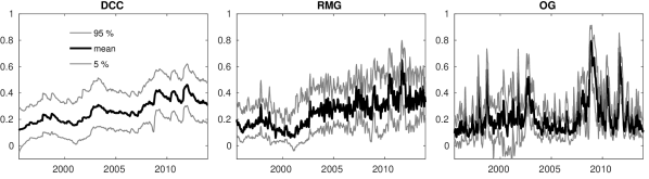
Figure 7: Averaged correlation as function of time. The figure shows the mean as well as the 90% bands of correlation coefficients obtained for the DCC, RMG, and OG model. For the calculation of all correlations 10-day non-overlapping windows have been applied.

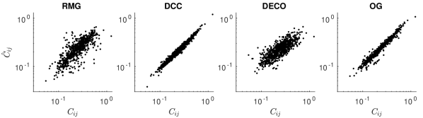
Figure 8: Covariances of simulated returns versus covariances of empirical returns. For better visibility we plot $C_{ij}$ for only 792 randomly chosen pairs of stocks on a log-log scale.

In the following we compare the covariances obtained from the RMG model with those obtained from the DCC, OG and DECO model and those implied by the empirical data. The form of $H_{t}$ in RMG, OG and DECO is in each case in some way restricted, which influences the estimated covariances. We therefore consider the standard DCC model, applied to subsamples of the data, as a benchmark estimation.

Even if the DCC model allows relatively large $N$, it is not designed for a sample like ours. It is typically applied for (and works best) for $N\leq 10$ (see Pakel et al., 2017; Zhang and Chan, 2009). For approaches to overcome this problem by using modified estimators, composite likelihood and shrinkage methods we refer the reader to Aielli (2013) and Engle et al. (2018).

For computational reasons the comparisons in this section (with exception of figure 7) are based on subsamples of covariances. We apply the DCC model to blocks of 8 stocks. The division of the stocks into these blocks is random. With a total number of 44 blocks we cover 352 stocks and 1,232 covariances. The RMG, OG and DECO model have been estimated for the entire sample of stocks, the comparison of covariances however is always based on the exact same 1,232 covariances. By repeating the sampling we have verified that the results presented in this section do not depend on the sampling.

Figure 7 shows the average correlation $\rho(t)$ together with the 90% interval for DCC, RMG and OG. The average correlation from DECO (not shown) is almost identical to that of the DCC model. The overall dynamics of the DCC and the RMG model seem to be rather similar. RMG exhibits larger fluctuations since it describes all pairs with 6 parameters. The OG model leads to qualitatively very different dynamics of the correlations.

	RMG	DECO	DCC	OG
$RMSE(\hat{C}_{ij}-C_{ij})$	2.1390	3.0633	1.4018	0.9513
$<|\hat{C}_{ij}-C_{ij})|>$	6.88 $\%$	11.03 $\%$	5.97 $\%$	4.44 $\%$
$<\Delta(\hat{r}_{i}\hat{r}_{j},r_{i}r_{j})>$	0.0091	0.0570	0.0558	0.1395
$std(\cdot)$	0.079	0.031	0.031	0.054
$<|\Delta(\hat{r}_{i}\hat{r}_{j},r_{i}r_{j})|>$	0.0650	0.0575	0.0562	0.1395
$std(\cdot)$	0.046	0.030	0.030	0.054

Table 2: The upper part of the table shows the differences between the estimated versus the empirical covariances. We also report the average percentage deviation of this difference with respect to $C_{ij}$. The bottom part of the table reports the differences in the distributions of the covariances, applying Cliff’s delta test. The first line gives the average value, the second line the average absolute difference together with the standard deviation.

We can judge whether the models lead to a correct description of the covariances by confronting them with the empirical data. For the conditional covariances perform the Monte Carlo simulation described in section 3 to obtain time averaged covariances $\hat{C}_{ij}$ and distributions of $\hat{r}_{i}\hat{r}_{j}$.

In figure 8 we show scatterplots comparing $\hat{C}_{ij}$ for the models with the observed time averaged covariances $C_{ij}$. Since $C$ is input in OG and is used for the mean of $H$ in DCC by covariance targeting we observe almost straight lines broadened by noise for these two cases. The somewhat larger deviation seen for RMG is partly due to the systematic error of the random matrix $C$. In RMG only the properties of the large eigenvalue of $C$ are used. The performance of DECO is similar and is caused due by the assumed stock-independent correlation. We can quantify this observation by calculating the differences between simulated and empirical covariances as $RMSE(C_{ij}-\hat{C}_{ij})$ given in the top part of table 2.

A more interesting comparison is to look at the distributions of the covariances. These distributions have pronounced peaks around 0 which are very dominant but not very decisive for our comparison. We have therefore decided to look at absolute covariances, in particular $\log(|r_{i}r_{j}|)$ for $|r_{i}r_{j}|>0$. Three examples for this distribution are shown in the figure in appendix E.

We measure the difference between the predicted distributions and those given by the data by calculating Cliff (1999)’s delta, denoted by $\Delta$. This statistic relies on comparing the elements in both distributions and counting how often each element is larger (smaller) than any element from the other distribution. Delta is bound within [-1,1], a value of 0 signals distributions that are indistinguishable while positive (negative) values signal some degree of imperfection in the overlap of the two distributions.

$$\Delta_{ij}=\frac{1}{n_{t}n_{\tau}}\sum_{t,\tau}\boldsymbol{[}|\hat{r}_{i}\hat{r}_{j}(\tau)|>|r_{i}r_{j}(t)|\boldsymbol{]}-\boldsymbol{[}|\hat{r}_{i}\hat{r}_{j}(\tau)|<|r_{i}r_{j}(t)|\boldsymbol{]}$$ (26)

In the bottom part of table 2 we report the mean of $\Delta$ and $|\Delta|$. Their standard deviation are a measure of the uncertainty. RMG has a $\Delta$ compatible with zero, while the values of DECO and DCC are slightly larger than zero. The dispersion of $\Delta$ however is larger for RMG than for the other models. Judging by the absolute $\Delta$ we can see that RMG achieves results that are only marginally behind DECO and DCC. The OG model for comparison performs noticeably worse.

5 Applications

5.1 Market transition

The large number of stocks in our sample allows to search for group specific regularities. An obvious question is if the correlations that can be extracted from $H(t)$ differ for stocks from specific sectors, and more interestingly, how they develop over time. Our sample period covers a time period during which we have seen pronounced changes in the market, including the IT bubble and the financial crisis. The visual inspection of some stocks’ betas in section 4 has already hinted at changes in the IT and the financial sector, which we want to analyze in more detail. For this reason we use the estimated $H(t)$ and then derive the conditional correlation matrices from $D^{-1}H(t)D^{-1}$ , where $D$ is a diagonal matrix with the square root of $H_{ii}(t)$ on the main diagonal. We can use these correlations to calculate the median correlation for pairs of stocks from specific sectors (GICS classification).

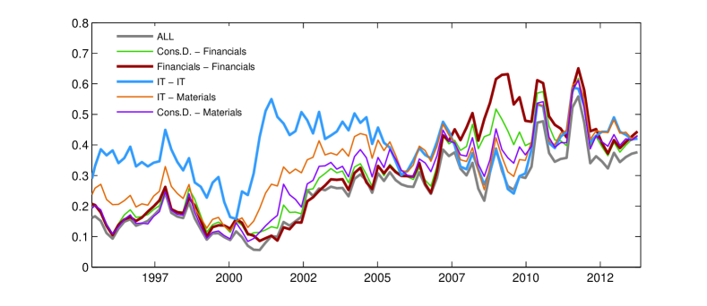
Figure 9: Development of median correlation by sector, averaged over 50 days. We show the average of all stock correlations (bold gray line), as well as some of the sectors with the strongest correlations. The sector with the strongest inter-sector correlation has for a long time been the IT sector (blue), later the financial sector (red) has taken over this role.

Figure 9 shows some of these median correlations. We observe very high average within-sector-correlations for stocks in the IT and financial sector. But also some correlations between stocks of different sectors are rather high, for example when the consumer or materials sectors are involved.

In general we observe two important changes over time. First, the overall level of correlations has shifted upwards from 2002 until 2007. The second observation is that the relative contribution of different sectors to overall correlation has changed. The most important change is that the financial sector surpasses the IT sector in terms of correlation around 2006.

These changes can be analyzed in more detail. In the analysis of Raddant and Wagner (2017) of the US, the UK, and the German stock market the same change has been found in the behavior based on the stock’s beta values, derived under the assumption that the covariance matrix of the returns has one large eigenvalue already at a time window sizes of 3 years. In the years 1994–2006 stocks with high trading volume and high beta mainly came from the information technology sector, whereas in 2006–2012 such stocks came mainly from the financial sector. Since a $\beta>1$ signals a risky investment, a market risk measure $\hat{R}(t,s)$ has been defined for the sectors $s$ by multiplying $\beta_{i}>1$ with the number $V(t,i)$ of traded shares in each time window.

$$\hat{R}(t,s)=A_{S}\sum_{i\epsilon s}\theta(\beta_{i}-1.0)\beta_{i}(t)\;V(t,i)$$ (27)

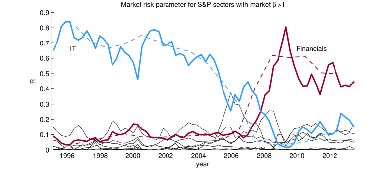
Figure 10: Time dependence of the risk parameter described in equation (27) for the sectors of the S&P market. The dashed line shows the result of Raddant and Wagner (2017). The solid lines (blue for the information technology and red for the financial sector) use daily $\beta$s from the RMG.

The normalization constant $A_{S}$ is chosen to have $\sum_{s}\;\hat{R}(t,s)=1$. When we apply this measure we see that before 2006 only the information technology sector and after 2006 only the financial sector exhibit large values of the risk measure.

However, the time and the duration of this transition had a systematic error of 1.5 years due to the window size. Repeating the calculation of $\hat{R}$ with the $\beta$ obtained from the RMG model serves two purposes. Firstly it is a check whether in RMG the market property can be reproduced and secondly the transition time can be determined more accurately, since daily $\beta$ are known from RMG. To reduce the noise on $\beta$ we average $\hat{R}(t,s)$ over one month. In figure 10 the risk parameters from equation (27) for the S&P market is shown as a function of time. The agreement with the previous determination (dashed lines) is good. With a time resolution of one month we can now safely say that the transition happens during the year 2006.

5.2 Leverage effect

The leverage effect consists in a negative correlation between volatility and future returns (Black, 1976; Bekaert and Wu, 2000). It is a relatively small effect (Schwert, 1989), but important for the estimation of risk. Since GARCH models provide a measurement of the daily volatility they are well suited for an analysis of this effect.

In a first step we determine for each stock the time correlation $L_{i}(t)$ between the market volatility $v_{0}$ and the observed returns $r_{ti}$:

$$L_{i}(t)=\frac{1}{N_{L}}\sum_{t^{\prime}}\left(v_{0}(t^{\prime}-t)-\bar{v_{0}}\right)r_{t^{\prime}i}$$ (28)

with the normalization factor $N_{L}^{2}=T\cdot var(v_{0})\sum_{t}r_{ti}^{2}$. Empirically the $L_{i}(t)\cdot sign(t)$ are dominantly negative with large fluctuations. To improve the sensitivity we use the asymmetry defined by

$$A_{i}=\frac{1}{t_{m}}\sum_{t=1}^{t_{m}}\big{(}L_{i}(t)-L_{i}(-t)\big{)}$$ (29)

with a maximum of the time lag $t_{m}$ of two months. $A_{i}$ corresponds to the difference in the area under $L(t)$ for positive and negative $t$. Due to the time symmetry of our model, using either $r_{ti}$ from equation (1) or the filtered returns $\eta_{G}$ should eliminate the leverage effect.

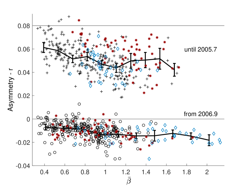
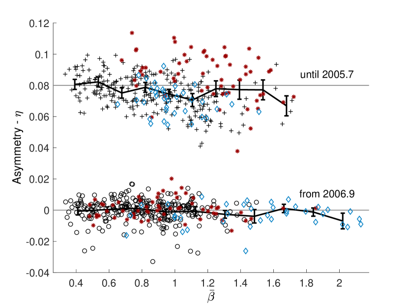
Figure 11: Asymmetry of $r$ vs $\bar{\beta}$ for stocks (left panel) and asymmetry of $\eta$ vs $\bar{\beta}$ (right panel) for all stocks. Blue diamonds refer to stocks from the technology sector, red stars to financials. The black line shows the average $\bar{\beta}$ and standard deviation. In both panels the upper part shows the result for the time period 1995–2005 and the lower part the results for 2007–2013.

It has been suggested by Black that the leverage effect is related to risk. To test this suggestion we show in the left panel of figure 11 the asymmetry as a function of the mean value $\bar{\beta}_{i}$. Since ${\beta(t)}$ changes around 2006 we use two time series, one covering the years 1995 until 2005 and a second one covering 2007 until 2013. The asymmetries are clearly negative and increase slightly with $\bar{\beta}$ as indicated by the line connecting the mean of $A$. By replacing $r_{t}$ by $\eta_{G}$ in equation (28) the effect should disappear. As shown in the right panel this is in fact the case.

The leverage effect can be included in the recursion. Analogous to the GJR-GARCH model (Glosten et al., 1993) an additional matrix proportional to $P_{\nu}(t)\;GJR\;P_{\nu^{\prime}}(t)$ with $GJR_{ij}=\delta_{ij}r_{ti}|r_{ti}|$ can be added on the r.h.s. of equation (37). For large $N$ the recursions for $v_{0}$ and $\beta$ are unchanged, only $v_{1}$ is affected. We repeated the fit including such a term. The likelihood improves, however the values of $\alpha$ and $\gamma$ are inside the errors the same. Also the results contained in figure 11 remain the same.

6 Conclusions

In our GARCH model we split the return into a market component and the remainder similar to a two-factor model. The parametrization of the covariance matrix $H$ avoids the numerical inversion of $H$. The small number of parameters and a computing time $T_{comp}\propto N$ allow the application to markets with a large number of stocks. The off-diagonal elements of our $H(t)$ have a precision that is competitive with other established models. Further, our model has the advantage that daily $\beta$ values relative to the market are determined. We found that replacing Gaussian by t-distributed noise is essential for the quality of the estimation results.

A possible development of the model would be to follow a similar strategy like DECO and to estimate univariate $h(t)$ in a first stage and to base the actual estimation of the model on residuals in a second stage.

Appendix

Appendix A Derivation of the recursions

We calculate $v_{k}(t+1)$ and $\beta(t+1)$ contained in the conditional covariance matrix

$$H(t+1)=Nv_{0}(t+1)P_{0}(t+1)+v_{1}(t+1)(I-P_{0}(t+1))$$ (30)

from the recursion (2.1)

$$H(t+1) = H(t)+\sum_{k=0,1}P_{k}(t)\left[\alpha_{k}\left(r(t)r^{\prime}(t)-H(t)\right)+\gamma_{k}\left(\bar{H}-H(t)\right)\right]P_{k}(t)$$ (31)

$$+ P_{0}(t)\left[\alpha_{10}r(t)r^{\prime}(t)+\gamma_{10}\bar{H}\right]P_{1}(t)$$

$$+ \;P_{1}(t)\left[\alpha_{10}r(t)r^{\prime}(t)+\gamma_{10}\bar{H}\right]P_{0}(t)$$

The mean $\bar{H}$ is given by equation (15). We apply the operation trace$P_{k}(t)\cdot$ on both sides of equation (31). The computation can be done using the algebraic properties of $P_{k}$ shown in equations (5) and (6). This leads to

$$\mbox{trace}H(t+1)P_{0}(t) = Nm^{2}(t)\;v_{0}(t+1)+{v_{1}(t+1)}(1-m^{2}(t))$$ (32)

$$= N\;R_{0}(t)$$

$$\mbox{trace}H(t+1)P_{1}(t) = N\;(1-m^{2}(t))\;v_{0}(t+1)+{v_{1}(t+1)}(N-2+m^{2}(t))$$ (33)

$$= N\;R_{1}(t)$$

where $m(t)=\beta^{\prime}(t+1)\cdot\beta(t)/N$ denotes the overlap between $\beta(t)$ and $\beta(t+1)$. The $R_{k}(t)$ represent the result of the same operation on the r.h.s. of equation (31) involving only the diagonal terms given by

$$R_{0}(t)=(1-\alpha_{0}-\gamma_{0})v_{0}(t)+\alpha_{0}r_{M}^{2}(t)+\frac{\gamma_{0}}{N}(N\bar{m}^{2}(t)\bar{v}_{0}-(1-\bar{m}^{2}(t))\bar{v}_{1})$$ (34)

$$R_{1}(t) = \frac{N-1}{N}(1-\alpha_{1}-\gamma_{1})v_{1}(t)+\alpha_{1}\bigl{(}\frac{r^{\prime}(t)r(t)}{N}-r_{M}^{2}(t)\bigr{)}$$ (35)

$$+ \frac{\gamma_{1}}{N}\bigl{(}N(1-\bar{m}^{2}(t))\bar{v}_{0}+(N-2+\bar{m}^{2}(t))\bar{v}_{1}\bigr{)}$$

The determination of the mean values $\bar{v}_{k}$ and $\bar{\beta}$ from $\bar{H}$ in equation (15) is described in appendix C. $\bar{m}(t)$ denotes the overlap between $\beta(t)$ and $\bar{\beta}$. Equations (33) and (34) determine $v_{k}(t+1)$ from the quantities $R_{k}(t)$ known at time $t$ and the overlap $m^{2}(t)$.

$$v_{0}(t+1)=\frac{1}{Nm^{2}(t)-1}\;\left[(N-2+m^{2}(t))R_{0}-(1-m^{2}(t))R_{1}\right]$$ (36)

$$v_{1}(t+1)=\frac{N}{Nm^{2}(t)-1}\;\left[m^{2}(t)R_{1}-(1-m^{2}(t))R_{0}\right]$$ (37)

To find $\beta(t+1)$ and thereby $m^{2}(t)$ we apply $H(t+1)$ to $\beta_{i}(t)$ and subtract $\beta_{i}(t)\;trace\;P_{0}(t)H(t+1)$ to obtain

$$\frac{1}{N}\bigl{(}(H(t+1)\beta)_{i}-\beta_{i}(t)\;trace\;H(t+1)P_{0}\bigr{)} =$$

$$w(t+1)\bigl{(}\beta_{i}(t+1)-m(t)\beta_{i}(t)\bigr{)} = D_{i}(t)$$ (38)

where we used the abbreviation $w(t)=v_{0}(t)-v_{1}(t)/N$. $D_{i}(t)$ represents the same operation on the r.h.s. of equation (31) involving only the non-diagonal terms. It is given by

$$D_{i}(t)=\alpha_{10}r_{M}(t)\bigl{(}r_{i}(t)-r_{M}(t)\beta_{i}(t)\bigr{)}+\gamma_{10}\;\bar{w}\;\bar{m}(t)\bigl{(}\bar{\beta}_{i}-\bar{m}(t)\beta_{i}(t)\bigr{)}$$ (39)

This leads to the following recursion for $\beta(t+1)$.

$$\beta_{i}(t+1)=m(t)\beta_{i}(t)+\frac{D_{i}(t)}{w(t+1)m(t)}$$ (40)

The unknown $m(t)$ follows from the normalization of $\beta^{\prime}(t+1)\cdot\beta(t+1)=N$. By some miracle the equation for $m(t)$ is only quadratic in $m^{2}(t)$ despite the complicated structure of equations (36) and (37). It reads

$$\left(R_{0}-\frac{R_{0}+R_{1}}{N}\right)^{2}m^{2}(t)(1-m^{2}(t))=\frac{D^{\prime}\cdot D}{N}\left(m^{2}(t)-\frac{1}{N}\right)^{2}$$ (41)

One of the two solutions with $Nm^{2}(t)\leq 1$ is to be excluded. Since $H(t+1)$ is insensitive to the sign of $\beta(t+1)$ we always have a positive overlap $m(t)$. With the correct solution of $m(t)$ the set of equations (36),(37),(40) and (41) yields $v_{k}(t+1)$ and $\beta(t+1)$ in terms of $r(t)$ and $\bar{H}$. The explicit solution looks rather complicated due to the dependence on $N$ in equation (41). For our purpose the limit $N\gg 1$ is sufficient. In this case we have

$$m^{2}(t)v_{0}(t+1)=R_{0}(t)$$ (42)

With $D_{i}(t)$ from equation (39) we get $m(t)$ by

$$m^{2}(t)=\left(1+\frac{D^{\prime}(t)\cdot D(t)}{NR^{2}_{0}(t)}\right)^{-1}$$ (43)

Finally $\beta(t+1)$ and $v_{1}(t+1)$ are found by

$$\beta_{i}(t+1)=m(t)\left(\beta_{i}(t)+\frac{D_{i}(t)}{R_{0}(t)}\right)$$ (44)

Inserting $R_{k}(t)$ leads to the formula given in section 2.

Necessary conditions on the GARCH parameters $\alpha_{k}$ and $\gamma_{k}$ are obtained by setting $r_{Mt}^{2}=\bar{v}_{0}$ and $r^{2}(t)=N(\bar{v}_{0}+\bar{v}_{1})$ to its mean values. Then the recursions have a fixed point $v_{k}(t)=\bar{v}_{k}$ and $\beta(t)=\bar{\beta}$ which is stable for

$$0<\gamma_{k}<\gamma_{k}+\alpha_{k}<1$$ (45)

Appendix B Calculation of the likelihood

The log likelihood with noise distribution $f(\varepsilon)$ can be computed using

$$\varepsilon(t)={H(t)}^{-1/2}r(t)$$ (46)

With a spectral decomposition for $H(t)$ functions of $H$ can be calculated analytically. For $H(t)^{-1/2}$ we obtain

$$H(t)^{-1/2}=\frac{1}{\sqrt{Nv_{0}(t)}}\;P_{0}(t)\;+\frac{1}{\sqrt{v_{1}(t)}}\;P_{1}(t)$$ (47)

It is easy to verify $(H(t)^{-1/2})^{2}\cdot H(t)=1$ with the orthogonality relations for $P_{\nu}(t)$. For $\varepsilon$ we obtain

$$\varepsilon(t)=\frac{r_{M}(t)}{\sqrt{Nv_{0}(t)}}\;\beta(t)\;+\;\frac{1}{\sqrt{v_{1}(t)}}\;(r(t)-r_{M}(t)\beta(t))$$ (48)

The log likelihood $L$ is given by

$$L=\frac{1}{2}\sum_{t}\left[\sum_{i}\ln f(\varepsilon_{i}(t))-\ln(Nv_{0}(t))-(N-1)\ln v_{1}(t)\right]$$ (49)

For Gaussian noise calculation of the $\ln(f)$ can be avoided. The complication of using t-distributed noise leads to an negligible increase of computing time compared to the calculation of $v_{\nu}(t)$ and $\beta(t)$. In any case the computing time increases only with $T\cdot N$.

Appendix C Covariance targeting for the restricted covariance matrix

For the time averaged covariance matrix $\tilde{C}$ of our model computed from

$$r(t)=\bar{H}^{1/2}\varepsilon(t)$$ (50)

we decompose the noise $\varepsilon$ into a component $\varepsilon_{M}(t)$ parallel to $\bar{\beta}$ and a component $\bar{\varepsilon}_{i}(t)$ perpendicular to $\bar{\beta}$. Both are i.i.d. with mean zero and variance one for large $N$. For $\tilde{C}$ we obtain

$$\tilde{C} = \frac{1}{T}\sum_{t}\left[N\;v_{0}(t)\;P_{0}(t)\;\varepsilon_{M}^{2}(t)+v_{1}(t)\;\bar{\varepsilon}(t)\bar{\varepsilon}^{\prime}(t)\right.$$ (51)

$$+ \left.\sqrt{v_{0}(t)v_{1}(t)}\;\varepsilon_{M}(t)(\beta(t)\bar{\varepsilon}^{\prime}(t)+\bar{\varepsilon}(t)\beta^{\prime}(t))\right]$$

The statistical uncertainty of $\tilde{C}$ is mainly due to the noise and much less due to the fluctuations of the slowly varying $v_{\nu}(t)$ and $\beta(t)$. For a rough estimate we neglect in the time average the $\varepsilon$-dependence in the latter. For the $tr(\tilde{C})$ we get for large $N$

$$tr(\tilde{C})=\frac{1}{T}\sum_{t}\left[N\;v_{0}(t)\;\varepsilon_{M}^{2}(t)+v_{1}(t)\;\sum_{i}\;\bar{\varepsilon}_{i}^{2}(t)\right]$$ (52)

The law of large numbers leads for the average over the noise to

$$tr(\tilde{C})=\frac{N}{T}\sum_{t}\;(v_{0}(t)\;+v_{1}(t))=N(\bar{v}_{0}+\bar{v}_{1})$$ (53)

where we replaced the time average of $v_{\nu}(t)$ by its mean $\bar{v}_{\nu}$. Comparing equation (53) with the observed covariance matrix gives one relation for $\bar{v}_{\nu}$ with a relative error of $1/\sqrt{T}$. The same procedure leads for the third term in equation (51) to a contribution of order $1/\sqrt{T}$ since the expectation value of $\bar{\varepsilon}_{i}(t)\;\varepsilon_{M}(t)$ vanishes. Replacing the second term $v_{1}(t)$ by $\bar{v_{1}}$ leads to a random matrix $R$ with a Marčenko-Pastur-spectrum. The average of the first term in equation (51) is equal to $N\bar{v}_{0}\bar{P}_{0}$. The resulting $\tilde{C}$ reads as

$$\tilde{C}=N\;\bar{v}_{0}\;\bar{P}_{0}\;+\;R$$ (54)

Since $|R_{ij}|<<N$ we can determine $\bar{v}_{0}$ and $\bar{\beta}$ by comparing the leading eigenvalue and eigenvector of $\tilde{C}$ and the observed $C$. The statistical error is in the order of $1/\sqrt{T}$.

Appendix D Experimental distributions

For comparing empirical data with simulations we apply a qualitative criterion which allows to locate eventual disagreement and is less sensitive to systematic errors as outliers. We assume $T$ independent measurements of an observable $x(t)\;(t=1,T)$. The values $x(t)$ are binned into $M$ bins of width $\Delta x_{m}$ centered around $x_{m}$ containing $n_{m}$ events. The probability density $f_{m}$ at $x_{m}$ is given by the relative frequency

$$f_{m}=\frac{1}{\Delta x_{m}}\;\frac{n_{m}}{T}$$ (55)

Errors of $f_{m}$ can be estimated assuming a Gaussian distribution by

$$\Delta f_{m}=\frac{1}{\sqrt{n_{m}-1}}\;f_{m}$$ (56)

Good plots of the distribution can be achieved by varying $\Delta x_{m}$ and by using a minimum for $n_{m}\geq 6$. In this way the empirical distributions in figures 1, 2, and 6 were created.

To estimate the quality of agreement of $f_{m}$ with a simulated density $F(x)$ we adopt the following qualitative measure: the average mean squared deviation also called $\chi^{2}$ ratio

$$\chi^{2}=\frac{1}{M}\sum_{m=1}^{M}\;\left(\frac{F(x_{m})-f_{m}}{\Delta f_{m}}\right)^{2}$$ (57)

A value of $\chi^{2}<4$ can be interpreted as agreement with 5% confidence level and values of $\chi^{2}<10$ still signal qualitative agreement.

Appendix E Distributions of covariances

For a visual comparison of the distributions we use the variable $\log(|r_{i}r_{j}|)$ for $|r_{i}r_{j}|>0$ in order to be sensitive to large values of $r_{i}r_{j}$ and not to be overwhelmed by the many small $r_{i}r_{j}$. Three typical examples of these distributions for pairs of stocks are shown in figure 12. The results for OG are often outside the empirical errors, whereas RMG and DECO agree with DCC and the data.

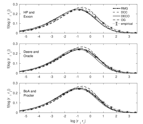
Figure 12: Simulated distributions of covariances. We show the distributions of the predicted covariances versus the original data. The dotted line connects the empirical pdf and a two standard deviations range. The broken and dotted black line corresponds to the simulated predicted correlations of RMG. The results for the DCC model are represented by the broken gray line The DECO model is represented by the gray line and the OGarch model by the broken black line. Note that the horizontal axis shows the logarithm of the absolute values of $r_{i}r_{j}$, therefore cases where the correlation is 0 are omitted.

References

- Aielli (2013) Gian Piero Aielli. Dynamic conditional correlation: On properties and estimation. Journal of Business & Economic Statistics, 31(3):282–299, 2013.
- Alexander (2001) Carol Alexander. A primer on the orthogonal GARCH model. mimeo, 2001.
- Bauwens et al. (2006) Luc Bauwens, Sébastien Laurent, and Jeroen V.K. Rombouts. Multivariate GARCH models: a survey. Journal of Applied Econometrics, 21(1):79–109, 2006.
- Bekaert and Wu (2000) Geert Bekaert and Guojun Wu. Asymmetric volatility and risk in equity markets. The Review of Financial Studies, 13(1):1–42, 2000.
- Black (1976) Fischer Black. Studies of stock market volatility changes. Proceedings of the American Statistical Association, Business and Economic Statistics Section, pages 177–181, 1976.
- Bollerslev et al. (1988) Tim Bollerslev, Robert F. Engle, and Jeffry M. Wooldridge. A capital asset pricing model with time-varying covariances. Journal of Political Economy, 96(1):116–131, 1988.
- Bollerslev et al. (1992) Tim Bollerslev, Ray Y. Chou, and Kenneth F. Kroner. ARCH modeling in finance. Journal of Econometrics, 52:5–59, 1992.
- Cliff (1999) Norman Cliff. Dominance statistics: Ordinal analyses to answer ordinal questions. Psychological Bulletin, 114(3):1–42, 1999.
- Ding and Engle (2001) Zhuanxin Ding and Robert F. Engle. Large scale conditional covariance matrix modeling, estimation and testing. working paper FLN-01-029, NYU Stern School of Business, 2001.
- Engle (2016) Robert F. Engle. Dynamic conditional beta. Journal of Financial Econometrics, 14(4):643–667, 2016.
- Engle and Kelly (2012) Robert F. Engle and Bryan Kelly. Dynamic equicorrelation. Journal of Business & Economic Statistics, 30:212–228, 2012.
- Engle and Kroner (1995) Robert F. Engle and Kenneth F. Kroner. Multivariate simultaneous generalized ARCH. Economic Theory, 11:122–150, 1995.
- Engle and Mezrich (1996) Robert F. Engle and Joseph Mezrich. GARCH for groups. Risk, 9:36–40, 1996.
- Engle et al. (2018) Robert F. Engle, Olivier Ledoit, and Michael Wolf. Large dynamic covariance matrices. Journal of Business & Economic Statistics, in press, 2018.
- Glosten et al. (1993) Lawrence R. Glosten, Ravi Jagannathan, and David E. Runkle. On the relation between the expected value and the volatility of the nominal excess return on stocks. The Journal of Finance, 48(5):1779–1801, 1993.
- Laloux et al. (1999) Laurent Laloux, Pierre Cizeau, Jean-Philippe Bouchaud, and Marc Potters. Noise dressing of financial correlation matrices. Phys.Rev.Lett., 83:1467, 1999.
- Lin (1992) Wen-Ling Lin. Alternative estimators for factor garch models – a monte carlo comparison. Journal of Applied Econometrics, 7:259–279, 1992.
- Lintner (1965) John Lintner. The valuation of risk assets and the selection of risky investments in stock portfolios and capital budgets. Review of Economics and Statistics, 47:13–37, 1965.
- Marčenko and Pastur (1967) Vladimir A. Marčenko and Leonid A. Pastur. Distribution of eigenvalues for some sets of random matrices. Mat. Sb. (N.S.), 72(114)(4):507–536, 1967.
- Pakel et al. (2017) Cavit Pakel, Neil Shephard, Kevin Sheppard, and Robert F. Engle. Fitting vast dimensional time-varying covariance models. NYU working paper, 2017.
- Raddant and Wagner (2017) Matthias Raddant and Friedrich Wagner. Transitions in the stock markets of the US, UK and Germany. Quantitative Finance, 17(2):289–297, 2017.
- Schwert (1989) G. William Schwert. Why does stock market volatility change over time? The Journal of Finance, 44(5):1115–1153, 1989.
- Sharpe (1964) William F. Sharpe. Capital asset prices: A theory of market equilibrium under conditions of risk. Journal of Finance, 19:425–442, 1964.
- van der Weide (2002) Roy van der Weide. GO-GARCH: A multivariate generalized orthogonal Garch model. Journal of Applied Econometrics, 17:549–564, 2002.
- Vrontos et al. (2003) I.D. Vrontos, P. Dellaportas, and D.N. Politis. A full-factor multivariate GARCH model. Econometrics Journal, 6:312–334, 2003.
- Wagner et al. (2010) Friedrich Wagner, Mishael Milaković, and Simone Alfarano. What distinguishes individual stocks from the index? Eur. Phys. J. B, 73:23–28, 2010.
- Zhang and Chan (2009) Kun Zhang and Laiwan Chan. Efficient factor GARCH models and factor-DCC models. Quantitative Finance, 9(1):71–91, 2009.