Nonparametric Bayesian Topic Modelling with the Hierarchical Pitman-Yor Processes

Abstract

The Dirichlet process and its extension, the Pitman-Yor process, are stochastic processes that take probability distributions as a parameter. These processes can be stacked up to form a hierarchical nonparametric Bayesian model. In this article, we present efficient methods for the use of these processes in this hierarchical context, and apply them to latent variable models for text analytics. In particular, we propose a general framework for designing these Bayesian models, which are called topic models in the computer science community. We then propose a specific nonparametric Bayesian topic model for modelling text from social media. We focus on tweets (posts on Twitter) in this article due to their ease of access. We find that our nonparametric model performs better than existing parametric models in both goodness of fit and real world applications.

Keywords: Bayesian nonparametric methods, Markov chain Monte Carlo, topic models, hierarchical Pitman-Yor processes, Twitter network modelling

1 Introduction

We live in the information age. With the Internet, information can be obtained easily and almost instantly. This has changed the dynamic of information acquisition, for example, we can now (1) attain knowledge by visiting digital libraries, (2) be aware of the world by reading news online, (3) seek opinions from social media, and (4) engage in political debates via web forums. As technology advances, more information is created, to a point where it is infeasible for a person to digest all the available content. To illustrate, in the context of a healthcare database (PubMed), the number of entries has seen a growth rate of approximately 3,000 new entries per day in the ten-year period from 2003 to 2013 (Suominen et al., 2014). This motivates the use of machines to automatically organise, filter, summarise, and analyse the available data for the users. To this end, researchers have developed various methods, which can be broadly categorised into computer vision (Low, 1991; Mai, 2010), speech recognition (Rabiner and Juang, 1993; Jelinek, 1997), and natural language processing (NLP, Manning and Schütze, 1999; Jurafsky and Martin, 2000). This article focuses on text analysis within NLP.

In text analytics, researchers seek to accomplish various goals, including sentiment analysis or opinion mining (Pang and Lee, 2008; Liu, 2012), information retrieval (Manning et al., 2008), text summarisation (Lloret and Palomar, 2012), and topic modelling (Blei, 2012). To illustrate, sentiment analysis can be used to extract digestible summaries or reviews on products and services, which can be valuable to consumers. On the other hand, topic models attempt to discover abstract topics that are present in a collection of text documents.

Topic models were inspired by latent semantic indexing (LSI, Landauer et al., 2007) and its probabilistic variant, probabilistic latent semantic indexing (pLSI), also known as the probabilistic latent semantic analysis (pLSA, Hofmann, 1999). Pioneered by Blei et al. (2003), latent Dirichlet allocation (LDA) is a fully Bayesian extension of pLSI, and can be considered the simplest Bayesian topic model. The LDA is then extended to many different types of topic models. Some of them are designed for specific applications (Wei and Croft, 2006; Mei et al., 2007), some of them model the structure in the text (Blei and Lafferty, 2006; Du, 2012), while some incorporate extra information in their modelling (Ramage et al., 2009; Jin et al., 2011).

On the other hand, due to the well known correspondence between the Gamma-Poisson family of distributions and the Dirichlet-multinomial family, Gamma-Poisson factor models (Canny, 2004) and their nonparametric extensions, and other Poisson-based variants of non-negative matrix factorisation (NMF) form a methodological continuum with topic models. These NMF methods are often applied to text, however, we do not consider these methods here.

This article will concentrate on topic models that take into account additional information. This information can be auxiliary data (or metadata) that accompany the text, such as keywords (or tags), dates, authors, and sources; or external resources like word lexicons. For example, on Twitter, a popular social media platform, its messages, known as tweets, are often associated with several metadata like location, time published, and the user who has written the tweet. This information is often utilised, for instance, Kinsella et al. (2011) model tweets with location data, while Wang et al. (2011b) use hashtags for sentiment classification on tweets. On the other hand, many topic models have been designed to perform bibliographic analysis by using auxiliary information. Most notable of these is the author-topic model (ATM, Rosen-Zvi et al., 2004), which, as its name suggests, incorporates authorship information. In addition to authorship, the Citation Author Topic model (Tu et al., 2010) and the Author Cite Topic Model (Kataria et al., 2011) make use of citations to model research publications. There are also topic models that employ external resources to improve modelling. For instance, He (2012) and Lim and Buntine (2014) incorporate a sentiment lexicon as prior information for a weakly supervised sentiment analysis.

Independent to the use of auxiliary data, recent advances in nonparametric Bayesian methods have produced topic models that utilise nonparametric Bayesian priors. The simplest examples replace Dirichlet distributions by the Dirichlet process (DP, Ferguson, 1973). The simplest is hierarchical Dirichlet process LDA (HDP-LDA) proposed by Teh et al. (2006) that replaces just the document by topic matrix in LDA. One can further extend topic models by using the Pitman-Yor process (PYP, Ishwaran and James, 2001) that generalises the DP, by replacing the second Dirichlet distribution which generates the topic by word matrix in LDA. This includes the work of Sato and Nakagawa (2010), Du et al. (2012b), Lindsey et al. (2012), among others. Like the HDP, the PYPs can be stacked to form hierarchical Pitman-Yor processes (HPYP), which are used in more complex models. Another fully nonparametric extension to topic modelling uses the Indian buffet process (Archambeau et al., 2015) to sparsify both the document by topic matrix and the topic by word matrix in LDA.

Advantages of employing nonparametric Bayesian methods with topic models is the ability to estimate the topic and word priors and to infer the number of clusters from the data. Using the PYP also allows the modelling of the power-law property exhibited by natural languages (Goldwater et al., 2005). These touted advantages have been shown to yield significant improvements in performance (Buntine and Mishra, 2014). However, we note the best known approach for learning with hierarchical Dirichlet (or Pitman-Yor) processes is to use the Chinese restaurant franchise (Teh and Jordan, 2010). Because this requires dynamic memory allocation to implement the hierarchy, there has been extensive research in attempting to efficiently implement just the HDP-LDA extension to LDA mostly based around variational methods (Teh et al., 2008; Wang et al., 2011a; Bryant and Sudderth, 2012; Sato et al., 2012; Hoffman et al., 2013). Variational methods have rarely been applied to more complex topic models, as we consider here, and unfortunately Bayesian nonparametric methods are gaining a reputation of being difficult to use. A newer collapsed and blocked Gibbs sampler (Chen et al., 2011) has been shown to generally outperform the variational methods as well as the original Chinese restaurant franchise in both computational time and space and in some standard performance metrics (Buntine and Mishra, 2014). Moreover, the technique does appear suitable for more complex topic models, as we consider here.

This article, extending the algorithm of Chen et al. (2011), shows how to develop fully nonparametric and relatively efficient Bayesian topic models that incorporate auxiliary information, with a goal to produce more accurate models that work well in tackling several applications. As a by-product, we wish to encourage the use of state-of-the-art Bayesian techniques, and also to incorporate auxiliary information, in modelling.

The remainder of this article is as follows. We first provide a brief background on the Pitman-Yor process in Section 2. Then, in Section 3, we detail our modelling framework by illustrating it on a simple topic model. We continue through to the inference procedure on the topic model in Section 4. Finally, in Section 5, we present an application on modelling social network data, utilising the proposed framework. Section 6 concludes.

2 Background on Pitman-Yor Process

We provide a brief, informal review of the Pitman-Yor process (PYP, Ishwaran and James, 2001) in this section. We assume the readers are familiar with basic probability distributions (see Walck, 2007) and the Dirichlet process (DP, Ferguson, 1973). In addition, we refer the readers to Hjort et al. (2010) for a tutorial on Bayesian nonparametric modelling.

2.1 Pitman-Yor Process

The Pitman-Yor process (PYP, Ishwaran and James, 2001) is also known as the two-parameter Poisson-Dirichlet process. The PYP is a two-parameter generalisation of the DP, now with an extra parameter $\alpha$ named the discount parameter in addition to the concentration parameter $\beta$. Similar to DP, a sample from a PYP corresponds to a discrete distribution (known as the output distribution) with the same support as its base distribution $H$. The underlying distribution of the PYP is the Poisson-Dirichlet distribution (PDD), which was introduced by Pitman and Yor (1997).

The PDD is defined by its construction process. For $0\leq\alpha<1$ and $\beta>-\alpha$, let $V_{k}$ be distributed independently as follows:

$$(V_{k}\,|\,\alpha,\beta)\sim\mathrm{Beta}(1-\alpha,\beta+k\alpha)\,, \mathrm{for}\ k=1,2,3,\,\dots\,,$$ (1)

and define $(p_{1},p_{2},p_{3},\,\dots)$ as

$$p_{1} =V_{1}\,,$$ (2)

$$p_{k} =V_{k}\prod_{i=1}^{k-1}(1-V_{i})\,, \mathrm{for}\ k\geq 2\,.$$ (3)

If we let ${p}=(\tilde{p}_{1},\tilde{p}_{2},\tilde{p}_{3},\,\dots)$ be a sorted version of $(p_{1},p_{2},p_{3},\,\dots)$ in descending order, then ${p}$ is Poisson-Dirichlet distributed with parameter $\alpha$ and $\beta$:

$${p}\sim\mathrm{PDD}(\alpha,\beta)\,.$$ (4)

Note that the unsorted version $(p_{1},p_{2},p_{3},\,\dots)$ follows a $\mathrm{GEM}(\alpha,\beta)$ distribution, which is named after Griffiths, Engen and McCloskey (Pitman, 2006).

With the PDD defined, we can then define the PYP formally. Let $H$ be a distribution over a measurable space $(\mathcal{X},\mathcal{B})$, for $0\leq\alpha<1$ and $\beta>-\alpha$, suppose that ${p}=(p_{1},p_{2},p_{3},\,\dots)$ follows a PDD (or GEM) with parameters $\alpha$ and $\beta$, then PYP is given by the formula

$$p(x\,|\,\alpha,\beta,H)=\sum_{k=1}^{\infty}p_{k}\,\delta_{X_{k}}(x)\,, \mathrm{for}\ k=1,2,3,\,\dots\,,$$ (5)

where $X_{k}$ are independent samples drawn from the base measure $H$ and $\delta_{X_{k}}(x)$ represents probability point mass concentrated at $X_{k}$ (i.e., it is an indicator function that is equal to $1$ when $x=X_{k}$ and $0$ otherwise):

$$\delta_{x}(y)=\left\{\begin{array}[]{ll}1&\mbox{if }x=y\\ 0&\mbox{otherwise}~{}\,.\end{array}\right.$$ (8)

This construction, Equation (1), is named the stick-breaking process. The PYP can also be constructed using an analogue to Chinese restaurant process (which explicitly draws a sequence of samples from the base distribution). A more extensive review on the PYP is given by Buntine and Hutter (2012).

A PYP is often more suitable than a DP in modelling since it exhibits a power-law behaviour (when $\alpha\neq 0$), which is observed in natural languages (Goldwater et al., 2005; Teh and Jordan, 2010). The PYP has also been employed in genomics (Favaro et al., 2009) and economics (Aoki, 2008). Note that when the discount parameter $\alpha$ is $0$, the PYP simply reduces to a DP.

2.2 Pitman-Yor Process with a Mixture Base

Note that the base measure $H$ of a PYP is not necessarily restricted to a single probability distribution. $H$ can also be a mixture distribution such as

$$H=\rho_{1}H_{1}+\rho_{2}H_{2}+\dots+\rho_{n}H_{n}\,,$$ (9)

where $\sum_{i=1}^{n}\rho_{i}=1$ and $\{H_{1},\dots H_{n}\}$ is a set of distributions over the same measurable space $(\mathcal{X},\mathcal{B})$ as $H$.

With this specification of $H$, the PYP is also named the compound Poisson-Dirichlet process in Du (2012), or the doubly hierarchical Pitman-Yor process in Wood and Teh (2009). A special case of this is the DP equivalent, which is also known as the DP with mixed random measures in Kim et al. (2012). Note that we have assumed constant values for the $\rho_{i}$ , though of course we can go fully Bayesian and assign a prior distribution for each of them, a natural prior would be the Dirichlet distribution.

2.3 Remark on Bayesian Inference

Performing exact Bayesian inference on nonparametric models is often intractable due to the difficulty in deriving the closed-form posterior distributions. This motivates the use of Markov chain Monte Carlo (MCMC) methods (see Gelman et al., 2013) for approximate inference. Most notable of the MCMC methods are the Metropolis-Hastings (MH) algorithms (Metropolis et al., 1953; Hastings, 1970) and Gibbs samplers (Geman and Geman, 1984). These algorithms serve as a building block for more advanced samplers, such as the MH algorithms with delayed rejection (Mira, 2001). Generalisations of the MCMC method include the reversible jump MCMC (Green, 1995) and its delayed rejection variant (Green and Mira, 2001) can also be employed for Bayesian inference, however, they are out of the scope in this article.

Instead of sampling one parameter at a time, one can develop an algorithm that updates more parameters in each iteration, a so-called blocked Gibbs sampler (Liu, 1994). Also, in practice we are usually only interested in a certain subset of the parameters; in such cases we can sometimes derive more efficient collapsed Gibbs samplers (Liu, 1994) by integrating out the nuisance parameters. In the remainder of this article, we will employ a combination of the blocked and collapsed Gibbs samplers for Bayesian inference.

3 Modelling Framework with Hierarchical Pitman-Yor Process

In this section, we discuss the basic design of our nonparametric Bayesian topic models using thierarchical Pitman-Yor processes (HPYP). In particular, we will introduce a simple topic model that will be extended later. We discuss the general inference algorithm for the topic model and hyperparameter optimisation.

Development of topic models is fundamentally motivated by their applications. Depending on the application, a specific topic model that is most suitable for the task should be designed and used. However, despite the ease of designing the model, the majority of time is spent on implementing, assessing, and redesigning it. This calls for a better designing cycle/routine that is more efficient, that is, spending less time in implementation and more time in model design and development.

We can achieve this by a higher level implementation of the algorithms for topic modelling. This has been made possible in other statistical domains by BUGS (Bayesian inference using Gibbs sampling, Lunn et al., 2000) or JAGS (just another Gibbs sampler, Plummer, 2003), albeit with standard probability distributions. Theoretically, BUGS and JAGS will work on LDA; however, in practice, running Gibbs sampling for LDA with BUGS and JAGS is very slow. This is because their Gibbs samplers are uncollapsed and not optimised. Furthermore, they cannot be used in a model with stochastic processes, like the Gaussian process (GP) and DP.

Below, we present a framework that allows us to implement HPYP topic models efficiently. This framework allows us to test variants of our proposed topic models without significant reimplementation.

3.1 Hierarchical Pitman-Yor Process Topic Model

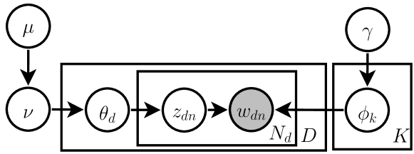
Figure 1: Graphical model of the HPYP topic model. It is an extension to LDA by allowing the probability vectors to be modelled by PYPs instead of the Dirichlet distributions. The area on the left of the graphical model (consists of $\mu$, $\nu$ and $\theta$) is usually referred as topic side, while the right hand side (with $\gamma$ and $\phi$) is called the vocabulary side. The word node denoted by $w_{dn}$ is observed. The notations are defined in Table 3.1.

The HPYP topic model is a simple network of PYP nodes since all distributions on the probability vectors are modelled by the PYP. For simplicity, we assume a topic model with three PYP layers, although in practice there is no limit to the number of PYP layers. We present the graphical model of our generic topic model in Figure 1. This model is a variant of those presented in Buntine and Mishra (2014), and is presented here as a starting model for illustrating our methods and for subsequent extensions.

At the root level, we have $\mu$ and $\gamma$ distributed as PYPs:

$$\mu \sim\mathrm{PYP}(\alpha^{\mu},\beta^{\mu},H^{\mu})\,,$$ (10)

$$\gamma \sim\mathrm{PYP}(\alpha^{\gamma},\beta^{\gamma},H^{\gamma})\,.$$ (11)

The variable $\mu$ is the root node for the topics in a topic model while $\gamma$ is the root node for the words. To allow arbitrary number of topics to be learned, we let the base distribution for $\mu$, $H^{\mu}$, to be a continuous distribution or a discrete distribution with infinite samples.

We usually choose a discrete uniform distribution for $\gamma$ based on the word vocabulary size of the text corpus. This decision is technical in nature, as we are able to assign a tiny probability to words not observed in the training set, which eases the evaluation process. Thus $H^{\gamma}=\{\cdots,\frac{1}{|\mathcal{V}|},\cdots\}$ where $|\mathcal{V}|$ is the set of all word vocabulary of the text corpus.

We now consider the topic side of the HPYP topic model. Here we have $\nu$, which is the child node of $\mu$. It follows a PYP given $\nu$, which acts as its base distribution:

$$\nu\sim\mathrm{PYP}(\alpha^{\nu},\beta^{\nu},\mu)\,.$$ (12)

For each document $d$ in a text corpus of size $D$, we have a document–topic distribution $\theta_{d}$ , which is a topic distribution specific to a document. Each of them tells us about the topic composition of a document.

$$\theta_{d}\sim\mathrm{PYP}(\alpha^{\theta_{d}},\beta^{\theta_{d}},\nu)\,, \mathrm{for\ \ }d=1,\dots,D\,.$$ (13)

While for the vocabulary side, for each topic $k$ learned by the model, we have a topic–word distribution $\phi_{k}$ which tells us about the words associated with each topic. The topic–word distribution $\phi_{k}$ is PYP distributed given the parent node $\gamma$, as follows:

$$\phi_{k}\sim\mathrm{PYP}(\alpha^{\phi_{k}},\beta^{\phi_{k}},\gamma)\,, \mathrm{for\ \ }k=1,\dots,K\,.$$ (14)

Here, $K$ is the number of topics in the topic model.

For every word $w_{dn}$ in a document $d$ which is indexed by $n$ (from $1$ to $N_{d}$ , the number of words in document $d$), we have a latent topic $z_{dn}$ (also known as topic assignment) which indicates the topic the word represents. $z_{dn}$ and $w_{dn}$ are categorical variables generated from $\theta_{d}$ and $\phi_{k}$ respectively:

$$z_{dn}\,|\,\theta_{d} \sim\mathrm{Discrete}(\theta_{d})\,,$$ (15)

$$w_{dn}\,|\,z_{dn},\phi \sim\mathrm{Discrete}(\phi_{z_{d}})\,, \mathrm{for\ \ }n=1,\dots,N_{d}\,.$$ (16)

The above $\alpha$ and $\beta$ are the discount and concentration parameters of the PYPs (see Section 2.1), note that they are called the hyperparameters in the model. We present a list of variables used in this section in Table 3.1.

Table 1: List of variables for the HPYP topic model used in this section.

Variable	Name	Description
$z_{dn}$	Topic	Topical label for word $w_{dn}$ .
$w_{dn}$	Word	Observed word or phrase at position $n$ in document $d$.
$\phi_{k}$	Topic–word distribution	Probability distribution in generating words for topic $k$.
$\theta_{d}$	Document–topic distribution	Probability distribution in generating topics for document $d$.
$\gamma$	Global word distribution	Word prior for $\phi_{k}$ .
$\nu$	Global topic distribution	Topic prior for $\theta_{d}$ .
$\mu$	Global topic distribution	Topic prior for $\nu$.
$\alpha^{\mathcal{N}}$	Discount	Discount parameter for PYP $\mathcal{N}$.
$\beta^{\mathcal{N}}$	Concentration	Concentration parameter for PYP $\mathcal{N}$.
$H^{\mathcal{N}}$	Base distribution	Base distribution for PYP $\mathcal{N}$.
$c^{\mathcal{N}}_{k}$	Customer count	Number of customers having dish $k$ in restaurant $\mathcal{N}$.
$t^{\mathcal{N}}_{k}$	Table count	Number of tables serving dish $k$ in restaurant $\mathcal{N}$.
$\mathbf{Z}$	All topics	Collection of all topics $z_{dn}$ .
$\mathbf{W}$	All words	Collection of all words $w_{dn}$ .
$\mathbf{\Xi}$	All hyperparameters	Collection of all hyperparameters and constants.
$\mathbf{C}$	All customer counts	Collection of all customers counts $c^{\mathcal{N}}_{k}$.
$\mathbf{T}$	All table counts	Collection of all table counts $t^{\mathcal{N}}_{k}$.

3.2 Model Representation and Posterior Likelihood

In a Bayesian setting, posterior inference requires us to analyse the posterior distribution of the model variables given the observed data. For instance, the joint posterior distribution for the HPYP topic model is

$$p(\mu,\nu,\gamma,\theta,\phi,\mathbf{Z}\,|\,\mathbf{W},\mathbf{\Xi})\,.$$ (17)

Here, we use bold face capital letters to represent the set of all relevant variables. For instance, $\mathbf{W}$ captures all words in the corpus. Additionally, we denote $\mathbf{\Xi}$ as the set of all hyperparameters and constants in the model.

Note that deriving the posterior distribution analytically is almost impossible due to its complex nature. This leaves us with approximate Bayesian inference techniques as mentioned in Section 2.3. However, even with these techniques, performing posterior inference with the posterior distribution is difficult due to the coupling of the probability vectors from the PYPs.

The key to an efficient inference procedure with the PYPs is to marginalise out the PYPs in the model and record various associated counts instead, which yields a collapsed sampler. To achieve this, we adopt a Chinese Restaurant Process (CRP) metaphor (Teh and Jordan, 2010; Blei et al., 2010) to represent the variables in the topic model. With this metaphor, all data in the model (e.g., topics and words) are the customers; while the PYP nodes are the restaurants the customers visit. In each restaurant, each customer is to be seated at only one table, though each table can have any number of customers. Each table in a restaurant serves a dish, the dish corresponds to the categorical label a data point may have (e.g., the topic label or word). Note that there can be more than one table serving the same dish. In a HPYP topic model, the tables in a restaurant $\mathcal{N}$ are treated as the customers for the parent restaurant $\mathcal{P}$ (in the graphical model, $\mathcal{P}$ points to $\mathcal{N}$), and they share the same dish. This means that the data is passed up recursively until the root node. For illustration, we present a simple example in Figure 2, showing the seating arrangement of the customers from two restaurants.

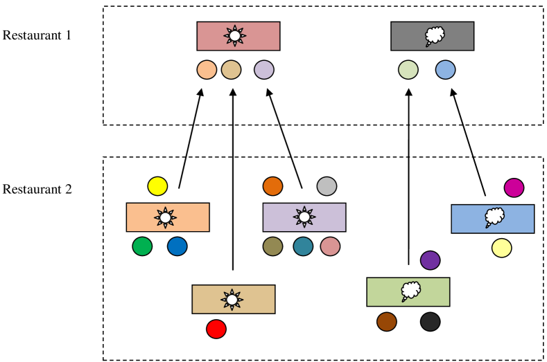
Figure 2: An illustration of the Chinese restaurant process representation. The customers are represented by the circles while the tables are represented by the rectangles. The dishes are the symbols in the middle of the rectangles, here they are denoted by the sunny symbol and the cloudy symbol. In this illustration, we know the number of customers corresponds to each table, for example, the green table is occupied by three customers. Also, since Restaurant 1 is the parent of Restaurant 2, the tables in Restaurant 2 are treated as the customers for Restaurant 1.

Naïvely recording the seating arrangement (table and dish) of each customer brings about computational inefficiency during inference. Instead, we adopt the table multiplicity (or table counts) representation of Chen et al. (2011) which requires no dynamic memory, thus consuming only a factor of memory at no loss of inference efficiency. Under this representation, we store only the customer counts and table counts associated with each restaurant. The customer count $c^{\mathcal{N}}_{k}$ denotes the number of customers who are having dish $k$ in restaurant $\mathcal{N}$. The corresponding symbol without subscript, $c^{\mathcal{N}}$, denotes the collection of customer counts in restaurant $\mathcal{N}$, that is, $c^{\mathcal{N}}=(\cdots,c^{\mathcal{N}}_{k},\cdots)$. The total number of customers in a restaurant $\mathcal{N}$ is denoted by the capitalised symbol instead, $C^{\mathcal{N}}=\sum_{k}c^{\mathcal{N}}_{k}$. Similar to the customer count, the table count $t^{\mathcal{N}}_{k}$ denotes the number of non-empty tables serving dish $k$ in restaurant $\mathcal{N}$. The corresponding $t^{\mathcal{N}}$ and $T^{\mathcal{N}}$ are defined similarly. For instance, from the example in Figure 2, we have $c^{2}_{\mathrm{sun}}=9$ and $t^{2}_{\mathrm{sun}}=3$, the corresponding illustration of the table multiplicity representation is presented in Figure 3. We refer the readers to Chen et al. (2011) for a detailed derivation of the posterior likelihood of a restaurant.

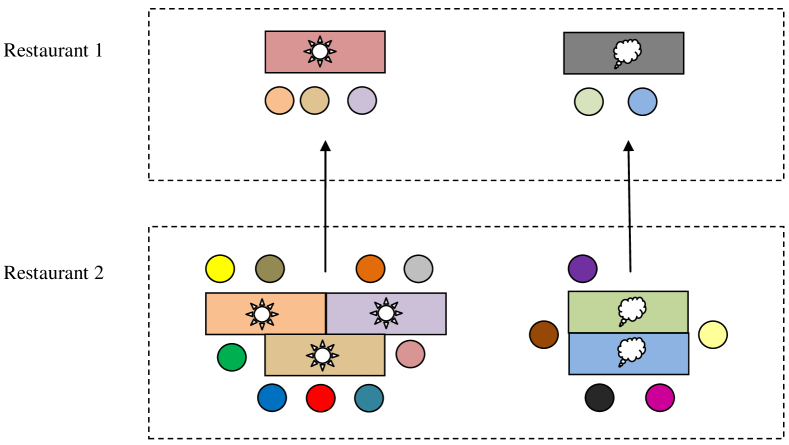
Figure 3: An illustration of the Chinese restaurant with the table counts representation. Here the setting is the same as Figure 2 but the seating arrangement of the customers are “forgotten” and only the table and customer counts are recorded. Thus, we only know that there are three sunny tables in Restaurant 2, with a total of nine customers.

For the posterior likelihood of the HPYP topic model, we marginalise out the probability vector associated with the PYPs and represent them with the customer counts and table counts, following Chen et al. (2011, Theorem 1). We present the modularised version of the full posterior of the HPYP topic model, which allows the posterior to be computed very quickly. The full posterior consists of the modularised likelihood associated with each PYP in the model, defined as

$$f(\mathcal{N}) =\frac{\big{(}\beta^{\mathcal{N}}\big{|}\alpha^{\mathcal{N}}\big{)}_{{T}^{\mathcal{N}}}}{\big{(}\beta^{\mathcal{N}}\big{)}_{C^{\mathcal{N}}}}\prod_{k=1}^{K}S^{c^{\mathcal{N}}_{k}}_{{t}^{\mathcal{N}}_{k},\,\alpha^{\mathcal{N}}}\binom{c^{\mathcal{N}}_{k}}{t^{\mathcal{N}}_{k}}^{-1}\,, \mathrm{for\ \ }\mathcal{N}\sim\mathrm{PYP}\big{(}\alpha^{\mathcal{N}},\beta^{\mathcal{N}},\mathcal{P}\big{)}\,.$$ (18)

Here, $S^{x}_{y,\,\alpha}$ are generalised Stirling numbers (Buntine and Hutter, 2012, Theorem 17). Both $(x)_{T}$ and $(x|y)_{T}$ denote Pochhammer symbols with rising factorials (Oldham et al., 2009, Section 18):

$$(x)_{T} =x\cdot(x+1)\cdots\big{(}x+(T-1)\big{)}~{}\,,$$ (19)

$$(x|y)_{T} =x\cdot(x+y)\cdots\big{(}x+(T-1)y\big{)}\,.$$ (20)

With the CRP representation, the full posterior of the HPYP topic model can now be written — in terms of $f(\cdot)$ given in Equation (18) — as

$$p(\mathbf{Z},\mathbf{T},\mathbf{C}\,|\,\mathbf{W},\mathbf{\Xi}) \propto p(\mathbf{Z},\mathbf{W},\mathbf{T},\mathbf{C}\,|\,\mathbf{\Xi})$$

$$\propto f(\mu)f(\nu)\Bigg{(}\prod_{d=1}^{D}f(\theta_{d})\!\Bigg{)}\Bigg{(}\prod_{k=1}^{K}f(\phi_{k})\!\Bigg{)}f(\gamma)\Bigg{(}\prod_{v=1}^{|\mathcal{V}|}\left(\frac{1}{|\mathcal{V}|}\right)^{t^{\gamma}_{v}}\Bigg{)}.$$ (21)

This result is a generalisation of Chen et al. (2011, Theorem 1) to account for discrete base distribution — the last term in Equation (21) corresponds to the base distribution of $\gamma$, and $v$ indexes each unique word in vocabulary set $\mathcal{V}$. The bold face $\mathbf{T}$ and $\mathbf{C}$ denote the collection of all table counts and customer counts, respectively. Note that the topic assignments $\mathbf{Z}$ are implicitly captured by the customer counts:

$$c^{\theta_{d}}_{k}=\sum_{n=1}^{N_{d}}I(z_{dn}=k)\,,$$ (22)

where $I(\cdot)$ is the indicator function, which evaluates to $1$ when the statement inside the function is true, and $0$ otherwise. We would like to point out that even though the probability vectors of the PYPs are integrated out and not explicitly stored, they can easily be reconstructed. This is discussed in Section 4.4. We move on to Bayesian inference in the next section.

4 Posterior Inference for the HPYP Topic Model

We focus on the MCMC method for Bayesian inference on the HPYP topic model. The MCMC method on topic models follows these simple procedures — decrementing counts contributed by a word, sample a new topic for the word, and update the model by accepting or rejecting the proposed sample. Here, we describe the collapsed blocked Gibbs sampler for the HPYP topic model. Note the PYPs are marginalised out so we only deal with the counts.

4.1 Decrementing the Counts Associated with a Word

The first step in a Gibbs sampler is to remove a word and corresponding latent topic, then decrement the associated customer counts and table counts. To give an example from Figure 2, if we remove the red customer from Restaurant 2, we would decrement the customer count $c^{2}_{\mathrm{sun}}$ by $1$. Additionally, we also decrement the table count $t^{2}_{\mathrm{sun}}$ by $1$ because the red customer is the only customer on its table. This in turn decrements the customer count $c^{1}_{\mathrm{sun}}$ by $1$. However, this requires us to keep track of the customers’ seating arrangement which leads to increased memory requirements and poorer performance due to inadequate mixing (Chen et al., 2011).

To overcome the above issue, we follow the concept of table indicator (Chen et al., 2011) and introduce a new auxiliary Bernoulli indicator variable $u^{\mathcal{N}}_{k}$, which indicates whether removing the customer also removes the table by which the customer is seated. Note that our Bernoulli indicator is different to that of Chen et al. (2011) which indicates the restaurant a customer contributes to. The Bernoulli indicator is sampled as needed in the decrementing procedure and it is not stored, this means that we simply “forget” the seating arrangements and re-sample them later when needed, thus we do not need to store the seating arrangement. The Bernoulli indicator of a restaurant $\mathcal{N}$ depends solely on the customer counts and the table counts:

$$p\big{(}u^{\mathcal{N}}_{k}\big{)}=\left\{\begin{array}[]{ll}t^{\mathcal{N}}_{k}/c^{\mathcal{N}}_{k}&~{}~{}\mathrm{if~{}~{}}u^{\mathcal{N}}_{k}=1\\[6.0pt] 1-t^{\mathcal{N}}_{k}/c^{\mathcal{N}}_{k}&~{}~{}\mathrm{if~{}~{}}u^{\mathcal{N}}_{k}=0~{}\,.\end{array}\right.$$ (25)

In the context of the HPYP topic model described in Section 3.1, we formally present how we decrement the counts associated with the word $w_{dn}$ and latent topic $z_{dn}$ from document $d$ and position $n$. First, on the vocabulary side (see Figure 1), we decrement the customer count $c^{\phi_{z_{dn}}}_{w_{dn}}$ associated with $\phi_{z_{dn}}$ by 1. Then sample a Bernoulli indicator $u^{\phi_{z_{dn}}}_{w_{dn}}$ according to Equation (25). If $u^{\phi_{z_{dn}}}_{w_{dn}}=1$, we decrement the table count $t^{\phi_{z_{dn}}}_{w_{dn}}$ and also the customer count $c^{\gamma}_{w_{dn}}$ by one. In this case, we would sample a Bernoulli indicator $u^{\gamma}_{w_{dn}}$ for $\gamma$, and decrement $t^{\gamma}_{w_{dn}}$ if $u^{\gamma}_{w_{dn}}=1$. We do not decrement the respective customer count if the Bernoulli indicator is $0$. Second, we would need to decrement the counts associated with the latent topic $z_{dn}$ . The procedure is similar, we decrement $c^{\theta_{d}}_{z_{dn}}$ by $1$ and sample the Bernoulli indicator $u^{\theta_{d}}_{z_{dn}}$ . Note that whenever we decrement a customer count, we sample the corresponding Bernoulli indicator. We repeat this procedure recursively until the Bernoulli indicator is $0$ or until the procedure hits the root node.

4.2 Sampling a New Topic for a Word

After decrementing the variables associated with a word $w_{dn}$ , we use a blocked Gibbs sampler to sample a new topic $z_{dn}$ for the word and the corresponding customer counts and table counts. The conditional posterior used in sampling can be computed quickly when the full posterior is represented in a modularised form. To illustrate, the conditional posterior for $z_{dn}$ and its associated customer counts and table counts is

$$p(z_{dn},\mathbf{T},\mathbf{C}\,|\,\mathbf{Z}^{-dn},\mathbf{W},\mathbf{T}^{-dn},\mathbf{C}^{-dn},\mathbf{\Xi})=\frac{p(\mathbf{Z},\mathbf{T},\mathbf{C}\,|\,\mathbf{W},\mathbf{\Xi})}{p(\mathbf{Z}^{-dn},\mathbf{T}^{-dn},\mathbf{C}^{-dn}\,|\,\mathbf{W},\mathbf{\Xi})}\,,$$ (26)

which is further broken down by substituting the posterior likelihood defined in Equation (21), giving the following ratios of the modularised likelihoods:

$$\frac{f(\mu)}{f(\mu^{-dn})}\frac{f(\nu)}{f(\nu^{-dn})}\frac{f(\theta_{d})}{f(\theta_{d}^{-dn})}\frac{f(\phi_{z_{dn}})}{f(\phi_{z_{dn}}^{-dn})}\frac{f(\gamma)}{f(\gamma^{-dn})}\left(\frac{1}{|\mathcal{V}|}\right)^{t^{\gamma}_{w_{dn}}-{(t^{\gamma}_{w_{dn}})}^{-dn}}\,.$$ (27)

The superscript $\Box^{-dn}$ indicates that the variables associated with the word $w_{dn}$ are removed from the respective sets, that is, the customer counts and table counts are after the decrementing procedure. Since we are only sample the topic assignment $z_{dn}$ associated with one word, the customer counts and table counts can only increment by at most $1$, see Table 2 for a list of all possible proposals.

Table 2: All possible proposals of the blocked Gibbs sampler for the variables associated with $w_{dn}$ . To illustrate, one sample would be $z_{dn}=1$, $t^{\mathcal{N}}_{z_{dn}}$ does not increment (stays the same), and $c^{\mathcal{N}}_{z_{dn}}$ increments by 1, for all $\mathcal{N}$ in $\{\mu,\nu,\theta_{d},\phi_{z_{dn}},\gamma\}$. We note that the proposals can include states that are invalid, but this is not an issue since those states have zero posterior probability and thus will not be sampled.

Variable	Possibilities	Variable	Possibilities	Variable	Possibilities
$z_{dn}$	$\{1,\dots,K\}$	$t^{\mathcal{N}}_{z_{dn}}$	$\{t^{\mathcal{N}}_{z_{dn}},\,t^{\mathcal{N}}_{z_{dn}}+1\}$	$c^{\mathcal{N}}_{z_{dn}}$	$\{c^{\mathcal{N}}_{z_{dn}},\,c^{\mathcal{N}}_{z_{dn}}+1\}$

This allows the ratios of the modularised likelihoods, which consists of ratios of Pochhammer symbol and ratio of Stirling numbers

$$\frac{f(\mathcal{N})}{f({\mathcal{N}}^{-dn})}=\frac{(\beta^{\mathcal{N}})_{{(C^{\mathcal{N}})}^{-dn}}}{(\beta^{\mathcal{N}})_{C^{\mathcal{N}}}}\frac{(\beta^{\mathcal{N}}|\alpha^{\mathcal{N}})_{{T}^{\mathcal{N}}}}{(\beta^{\mathcal{N}}|\alpha^{\mathcal{N}})_{{(T^{\mathcal{N}})}^{-dn}}}\prod_{k=1}^{K}\frac{S^{c^{\mathcal{N}}_{k}}_{{t}^{\mathcal{N}}_{k},\,\alpha^{\mathcal{N}}}}{S^{{(c^{\mathcal{N}}_{k})}^{-dn}}_{{(t^{\mathcal{N}}_{k})}^{-dn},\,\alpha^{\mathcal{N}}}}~{}\,,$$ (28)

to simplify further. For instance, the ratios of Pochhammer symbols can be reduced to constants, as follows:

$$\frac{(x)_{T+1}}{(x)_{T}}=x+T\,, \frac{(x|y)_{T+1}}{(x|y)_{T}}=x+yT\,.$$ (29)

The ratio of Stirling numbers, such as $S^{y+1}_{x+1,\,\alpha}/S^{y}_{x,\,\alpha}$ , can be computed quickly via caching (Buntine and Hutter, 2012). Technical details on implementing the Stirling numbers cache can be found in Lim (2016).

With the conditional posterior defined, we proceed to the sampling process. Our first step involves finding all possible changes to the topic $z_{dn}$ , customer counts, and the table counts (hereafter known as ‘state’) associated with adding the removed word $w_{dn}$ back into the topic model. Since only one word is added into the model, the customer counts and the table counts can only increase by at most $1$, constraining the possible states to a reasonably small number. Furthermore, the customer counts of a parent node will only be incremented when the table counts of its child node increases. Note that it is possible for the added customer to generate a new dish (topic) for the model. This requires the customer to increment the table count of a new dish in the root node $\mu$ by $1$ (from $0$).

Next, we compute the conditional posterior (Equation (26)) for all possible states. The conditional posterior (up to a proportional constant) can be computed quickly by breaking down the posterior and calculating the relevant parts. We then normalise them to sample one of the states to be the proposed next state. Note that the proposed state will always be accepted, which is an artifact of Gibbs sampler.

Finally, given the proposal, we update the HPYP model by incrementing the relevant customer counts and table counts.

4.3 Optimising the Hyperparameters

Choosing the right hyperparameters for the priors is important for topic models. Wallach et al. (2009a) show that an optimised hyperparameter increases the robustness of the topic models and improves their model fitting. The hyperparameters of the HPYP topic models are the discount parameters and concentration parameters of the PYPs. Here, we propose a procedure to optimise the concentration parameters, but leave the discount parameters fixed due to their coupling with the Stirling numbers cache.

The concentration parameters $\beta$ of all the PYPs are optimised using an auxiliary variable sampler similar to Teh (2006). Being Bayesian, we assume the concentration parameter $\beta^{\mathcal{N}}$ of a PYP node $\mathcal{N}$ has the following hyperprior:

$$\beta^{\mathcal{N}}\sim\mathrm{Gamma}(\tau_{0},\tau_{1})\,, \mathrm{for\ \ }\mathcal{N}\sim\mathrm{PYP}\big{(}\alpha^{\mathcal{N}},\beta^{\mathcal{N}},\mathcal{P}\big{)}\,,$$ (30)

where $\tau_{0}$ is the shape parameter and $\tau_{1}$ is the rate parameter. The gamma prior is chosen due to its conjugacy which gives a gamma posterior for $\beta^{\mathcal{N}}$.

To optimise $\beta^{\mathcal{N}}$, we first sample the auxiliary variables $\omega$ and $\zeta_{i}$ given the current value of $\alpha^{\mathcal{N}}$ and $\beta^{\mathcal{N}}$, as follows:

$$\omega\,|\,\beta^{\mathcal{N}} \sim\mathrm{Beta}\big{(}C^{\mathcal{N}},\beta^{\mathcal{N}}\big{)}\,,$$ (31)

$$\zeta_{i}\,|\,\alpha^{\mathcal{N}},\beta^{\mathcal{N}} \sim\mathrm{Bernoulli}\left(\frac{\beta^{\mathcal{N}}}{\beta^{\mathcal{N}}+i\alpha^{\mathcal{N}}}\right)\,, \mathrm{for\ \ }i=0,1,\dots,T^{\mathcal{N}}-1~{}\,.$$ (32)

With these, we can then sample a new $\beta^{\mathcal{N}}$ from its conditional posterior

$$\beta^{\mathcal{N}}\,\big{|}\,\omega,\zeta\sim\mathrm{Gamma}\left(\tau_{0}+\sum_{i=0}^{T^{\mathcal{N}}-1}\zeta_{i}~{}~{},~{}~{}\tau_{1}-\log(1-\omega)\right)~{}\,.$$ (33)

The collapsed Gibbs sampler is summarised by Algorithm 1.

Algorithm 1 Collapsed Gibbs Sampler for the HPYP Topic Model

1. Initialise the HPYP topic model by assigning random topic to the latent topic $z_{dn}$ associated to each word $w_{dn}$ . Then update all the relevant customer counts $\mathbf{C}$ and table counts $\mathbf{T}$ by using Equation (22) and setting the table counts to be about half of the customer counts.

2. For each word $w_{dn}$ in each document $d$, do the following:

   1. Decrement the counts associated with $w_{dn}$ (see Section 4.1).

   2. Block sample a new topic for $z_{dn}$ and corresponding customer counts $\mathbf{C}$ and table counts $\mathbf{T}$ (see Section 4.2).

   3. Update (increment counts) the topic model based on the sample.

3. Update the hyperparameter $\beta^{\mathcal{N}}$ for each PYP nodes $\mathcal{N}$ (see Section 4.3).

4. Repeat Steps 2 – 3 until the model converges or when a fix number of iterations is reached.

4.4 Estimating the Probability Vectors of the PYPs

Recall that the aim of topic modelling is to analyse the posterior of the model parameters, such as one in Equation (17). Although we have marginalised out the PYPs in the above Gibbs sampler, the PYPs can be reconstructed from the associated customer counts and table counts. Recovering the full posterior distribution of the PYPs is a complicated task. So, instead, we will analyse the PYPs via the expected value of their conditional marginal posterior distribution, or simply, their posterior mean,

$$\mathbb{E}[\mathcal{N}\,|\,\mathbf{Z},\mathbf{W},\mathbf{T},\mathbf{C},\mathbf{\Xi}]\,, \mathrm{for\ }\mathcal{N}\in\{\mu,\nu,\gamma,\theta_{d},\phi_{k}\}\,.$$ (34)

The posterior mean of a PYP corresponds to the probability of sampling a new customer for the PYP. To illustrate, we consider the posterior of the topic distribution $\theta_{d}$ . We let $\tilde{z}_{dn}$ to be a unknown future latent topic in addition to the known $\mathbf{Z}$. With this, we can write the posterior mean of $\theta_{dk}$ as

$$\mathbb{E}[\theta_{dk}\,|\,\mathbf{Z},\mathbf{W},\mathbf{T},\mathbf{C},\mathbf{\Xi}] =\mathbb{E}[p(\tilde{z}_{dn}=k\,|\,\theta_{d},\mathbf{Z},\mathbf{W},\mathbf{T},\mathbf{C},\mathbf{\Xi})\,|\,\mathbf{Z},\mathbf{W},\mathbf{T},\mathbf{C},\mathbf{\Xi}]$$

$$=\mathbb{E}[p(\tilde{z}_{dn}=k\,|\,\mathbf{Z},\mathbf{T},\mathbf{C})\,|\,\mathbf{Z},\mathbf{W},\mathbf{T},\mathbf{C},\mathbf{\Xi}]\,.$$ (35)

by replacing $\theta_{dk}$ with the posterior predictive distribution of $\tilde{z}_{dn}$ and note that $\tilde{z}_{dn}$ can be sampled using the CRP, as follows:

$$p(\tilde{z}_{dn}=k\,|\,\mathbf{Z},\mathbf{T},\mathbf{C})=\frac{(\alpha^{\theta_{d}}T^{\theta_{d}}+\beta^{\theta_{d}})\nu_{k}+c_{k}^{\theta_{d}}-\alpha^{\theta_{d}}T_{k}^{\theta_{d}}}{\beta^{\theta_{d}}+C^{\theta_{d}}}\,.$$ (36)

Thus, the posterior mean of $\theta_{d}$ is given as

$$\mathbb{E}[\theta_{dk}\,|\,\mathbf{Z},\mathbf{W},\mathbf{T},\mathbf{C},\mathbf{\Xi}]=\frac{(\alpha^{\theta_{d}}T^{\theta_{d}}+\beta^{\theta_{d}})\mathbb{E}[\nu_{k}\,|\,\mathbf{Z},\mathbf{W},\mathbf{T},\mathbf{C},\mathbf{\Xi}]+c_{k}^{\theta_{d}}-\alpha^{\theta_{d}}T_{k}^{\theta_{d}}}{\beta^{\theta_{d}}+C^{\theta_{d}}}\,,$$ (37)

which is written in term of the posterior mean of its parent PYP, $\nu$. The posterior means of the other PYPs such as $\nu$ can be derived by taking a similar approach. Generally, the posterior mean corresponds to a PYP $\mathcal{N}$ (with parent PYP $\mathcal{P}$) is as follows:

$$\mathbb{E}[\mathcal{N}_{k}\,|\,\mathbf{Z},\mathbf{W},\mathbf{T},\mathbf{C},\mathbf{\Xi}]=\frac{(\alpha^{\mathcal{N}}T^{\mathcal{N}}+\beta^{\mathcal{N}})\mathbb{E}[\mathcal{P}_{k}\,|\,\mathbf{Z},\mathbf{W},\mathbf{T},\mathbf{C},\mathbf{\Xi}]+c_{k}^{\mathcal{N}}-\alpha^{\mathcal{N}}T_{k}^{\mathcal{N}}}{\beta^{\mathcal{N}}+C^{\mathcal{N}}}\,,$$ (38)

By applying Equation (38) recursively, we obtain the posterior mean for all the PYPs in the model.

We note that the dimension of the topic distributions ($\mu$, $\nu$, $\theta$) is $K+1$, where $K$ is the number of observed topics. This accounts for the generation of a new topic associated with the new customer, though the probability of generating a new topic is usually much smaller. In practice, we may instead ignore the extra dimension during the evaluation of a topic model since it does not provide useful interpretation. One way to do this is to simply discard the extra dimension of all the probability vectors after computing the posterior mean. Another approach would be to normalise the posterior mean of the root node $\mu$ after discarding the extra dimension, before computing the posterior mean of others PYPs. Note that for a considerably large corpus, the difference in the above approaches would be too small to notice.

4.5 Evaluations on Topic Models

Generally, there are two ways to evaluate a topic model. The first is to evaluate the topic model based on the task it performs, for instance, the ability to make predictions. The second approach is the statistical evaluation of the topic model on modelling the data, which is also known as the goodness-of-fit test. In this section, we will present some commonly used evaluation metrics that are applicable to all topic models, but we first discuss the procedure for estimating variables associated with the test set.

4.5.1 Predictive Inference on the Test Documents

Test documents, which are used for evaluations, are set aside from learning documents. As such, the document–topic distributions ${\theta}$ associated with the test documents are unknown and hence need to be estimated. One estimate for ${\theta}$ is its posterior mean given the variables learned from the Gibbs sampler:

$$\hat{{\theta}}_{d}=\mathbb{E}[{\theta}_{d}\,|\,\mathbf{Z},\mathbf{W},\mathbf{T},\mathbf{C},\mathbf{\Xi}]\,,$$ (39)

obtainable by applying Equation (38). Note that since the latent topics $\tilde{\mathbf{Z}}$ corresponding to the test set are not sampled, the customer counts and table counts associated with ${\theta}_{d}$ are $0$, thus $\hat{{\theta}}_{d}$ is equal to $\hat{\nu}$, the posterior mean of $\nu$. However, this is not a good estimate for the topic distribution of the test documents since they will be identical for all the test documents. To overcome this issue, we will instead use some of the words in the test documents to obtain a better estimate for ${\theta}$. This method is known as document completion (Wallach et al., 2009b), as we use part of the text to estimate ${\theta}$, and use the rest for evaluation.

Getting a better estimate for ${\theta}$ requires us to first sample some of the latent topics $\tilde{z}_{dn}$ in the test documents. The proper way to do this is by running an algorithm akin to the collapsed Gibbs sampler, but this would be excruciatingly slow due to the need to re-sample the customer counts and table counts for all the parent PYPs. Instead, we assume that the variables learned from the Gibbs sampler are fixed and sample the $\tilde{z}_{dn}$ from their conditional posterior sequentially, given the previous latent topics:

$$p(\tilde{z}_{dn}=k\,|\,\tilde{w}_{dn},{\theta}_{d},\phi,\tilde{z}_{d1},\dots,\tilde{z}_{d,n-1})\propto{\theta}_{dk}\,\phi_{kw_{dn}}\,.$$ (40)

Whenever a latent topic $\tilde{z}_{dn}$ is sampled, we increment the customer count $c^{{\theta}_{d}}_{\tilde{z}_{dn}}$ for the test document. For simplicity, we set the table count $t^{{\theta}_{d}}_{\tilde{z}_{dn}}$ to be half the corresponding customer counts $c^{{\theta}_{d}}_{\tilde{z}_{dn}}$, this avoids the expensive operation of sampling the table counts. Additionally, ${\theta}_{d}$ is re-estimated using Equation (39) before sampling the next latent topic. We note that the estimated variables are unbiased.

The final ${\theta}_{d}$ becomes an estimate for the topic distribution of the test document $d$. The above procedure is repeated $R$ times to give $R$ samples of ${\theta}_{d}^{(r)}$, which are used to compute the following Monte Carlo estimate of ${\theta}_{d}$:

$$\hat{{\theta}}_{d}=\frac{1}{R}\sum_{r=1}^{R}{\theta}_{d}^{(r)}\,.$$ (41)

This Monte Carlo estimate can then be used for computing the evaluation metrics. Note that when estimating ${\theta}$, we have ignored the possibility of generating a new topic, that is, the latent topics $\tilde{z}$ are constrained to the existing topics, as previously discussed in Section 4.4.

4.5.2 Goodness-of-fit Test

Measures of goodness-of-fit usually involves computing the discrepancy of the observed values and the predicted values under the model. However, the observed variables in a topic model are the words in the corpus, which are not quantifiable since they are discrete labels. Thus evaluations on topic models are usually based on the model likelihoods instead.

A popular metric commonly used to evaluate the goodness-of-fit of a topic model is perplexity, which is negatively related to the likelihood of the observed words $\mathbf{W}$ given the model, this is defined as

$$\mathrm{perplexity}(\mathbf{W}\,|\,\theta,\phi)=\exp\Bigg{(}-\frac{\sum_{d=1}^{D}\sum_{n=1}^{N_{d}}\log p(w_{dn}\,|\,\theta_{d},\phi)}{\sum_{d=1}^{D}N_{d}}\Bigg{)}\,,$$ (42)

where $p(w_{dn}\,|\,\theta_{d},\phi)$ is the likelihood of sampling the word $w_{dn}$ given the document–topic distribution $\theta_{d}$ and the topic–word distributions $\phi$. Computing $p(w_{dn}\,|\,\theta_{d},\phi)$ requires us to marginalise out $z_{dn}$ from their joint distribution, as follows:

$$p(w_{dn}\,|\,\theta_{d},\phi) =\sum_{k}p(w_{dn},\,z_{dn}=k\,|\,\theta_{d},\phi)$$

$$=\sum_{k}p(w_{dn}\,|\,z_{dn}=k,\phi_{k})\,p(z_{dn}=k\,|\,\theta_{d})$$

$$=\sum_{k}\phi_{kw_{dn}}\theta_{dk}~{}\,.$$ (43)

Although perplexity can be computed on the whole corpus, in practice we compute the perplexity on test documents. This is to measure if the topic model generalises well to unseen data. A good topic model would be able to predict the words in the test set better, thereby assigning a higher probability $p(w_{dn}\,|\,\theta_{d},\phi)$ in generating the words. Since perplexity is negatively related to the likelihood, a lower perplexity is better.

4.5.3 Document Clustering

We can also evaluate the clustering ability of the topic models. Note that topic models assign a topic to each word in a document, essentially performing a soft clustering (Erosheva and Fienberg, 2005) for the documents in which the membership is given by the document–topic distribution $\theta$. To evaluate the clustering of the documents, we convert the soft clustering to hard clustering by choosing a topic that best represents the documents, hereafter called the dominant topic. The dominant topic of a document $d$ corresponds to the topic that has the highest proportion in the topic distribution, that is,

$$\mathrm{Dominant\ Topic}(\theta_{d})=\operatornamewithlimits{arg\,max}_{k}\theta_{dk}\,.$$ (44)

Two commonly used evaluation measures for clustering are purity and normalised mutual information (NMI, Manning et al., 2008). The purity is a simple clustering measure which can be interpreted as the proportion of documents correctly clustered, while NMI is an information theoretic measures used for clustering comparison. If we denote the ground truth classes as $\mathcal{S}=\{s_{1},\dots,s_{J}\}$ and the obtained clusters as $\mathcal{R}=\{r_{1},\dots,r_{K}\}$, where each $s_{j}$ and $r_{k}$ represents a collection (set) of documents, then the purity and NMI can be computed as

$$\mathrm{purity}(\mathcal{S},\mathcal{R})=\frac{1}{D}\sum_{k=1}^{K}\max_{j}|r_{k}\cap s_{j}|\,, \mathrm{NMI}(\mathcal{S},\mathcal{R})=\frac{2\,\mathrm{MI}(\mathcal{S};\mathcal{R})}{E(\mathcal{S})+E(\mathcal{R})}\,,$$ (45)

where $\mathrm{MI}(\mathcal{S};\mathcal{R})$ denotes the mutual information between two sets and $E(\cdot)$ denotes the entropy. They are defined as follows:

$$\mathrm{MI}(\mathcal{S};\mathcal{R})=\sum_{k=1}^{K}\sum_{j=1}^{J}\frac{|r_{k}\cap s_{j}|}{D}\log_{2}D\frac{|r_{k}\cap s_{j}|}{|r_{k}||s_{j}|}\,, E(\mathcal{R})=-\sum_{k=1}^{K}\frac{|r_{k}|}{D}\log_{2}\frac{|r_{k}|}{D}\,.$$ (46)

Note that the higher the purity or NMI, the better the clustering.

5 Application: Modelling Social Network on Twitter

This section looks at how we can employ the framework discussed above for an application of tweet modelling, using auxiliary information that is available on Twitter. We propose the Twitter-Network topic model (TNTM) to jointly model the text and the social network in a fully Bayesian nonparametric way, in particular, by incorporating the authors, hashtags, the “follower” network, and the text content in modelling. The TNTM employs a HPYP for text modelling and a Gaussian process (GP) random function model for social network modelling. We show that the TNTM significantly outperforms several existing nonparametric models due to its flexibility.

5.1 Motivation

Emergence of web services such as blogs, microblogs and social networking websites allows people to contribute information freely and publicly. This user-generated information is generally more personal, informal, and often contains personal opinions. In aggregate, it can be useful for reputation analysis of entities and products (Aula, 2010), natural disaster detection (Karimi et al., 2013), obtaining first-hand news (Broersma and Graham, 2012), or even demographic analysis (Correa et al., 2010). We focus on Twitter, an accessible source of information that allows users to freely voice their opinions and thoughts in short text known as tweets.

Although LDA (Blei et al., 2003) is a popular model for text modelling, a direct application on tweets often yields poor result as tweets are short and often noisy (Zhao et al., 2011; Baldwin et al., 2013), that is, tweets are unstructured and often contain grammatical and spelling errors, as well as informal words such as user-defined abbreviations due to the 140 characters limit. LDA fails on short tweets since it is heavily dependent on word co-occurrence. Also notable is that the text in tweets may contain special tokens known as hashtags; they are used as keywords and allow users to link their tweets with other tweets tagged with the same hashtag. Nevertheless, hashtags are informal since they have no standards. Hashtags can be used as both inline words or categorical labels. When used as labels, hashtags are often noisy, since users can create new hashtags easily and use any existing hashtags in any way they like. Hence instead of being hard labels, hashtags are best treated as special words which can be the themes of the tweets. These properties of tweets make them challenging for topic models, and ad hoc alternatives are used instead. For instance, Maynard et al. (2012) advocate the use of shallow method for tweets, and Mehrotra et al. (2013) utilise a tweet-pooling approach to group short tweets into a larger document. In other text analysis applications, tweets are often ‘cleansed’ by NLP methods such as lexical normalisation (Baldwin et al., 2013). However, the use of normalisation is also criticised (Eisenstein, 2013), as normalisation can change the meaning of text.

In the following, we propose a novel method for better modelling of microblogs by leveraging the auxiliary information that accompanies tweets. This information, complementing word co-occurrence, also opens the door to more applications, such as user recommendation and hashtag suggestion. Our major contributions include (1) a fully Bayesian nonparametric model named the Twitter-Network topic model (TNTM) that models tweets well, and (2) a combination of both the HPYP and the GP to jointly model text, hashtags, authors and the followers network. Despite the seeming complexity of the TNTM model, its implementation is made relatively straightforward using the flexible framework developed in Section 3. Indeed, a number of other variants were rapidly implemented with this framework as well.

5.2 The Twitter-Network Topic Model

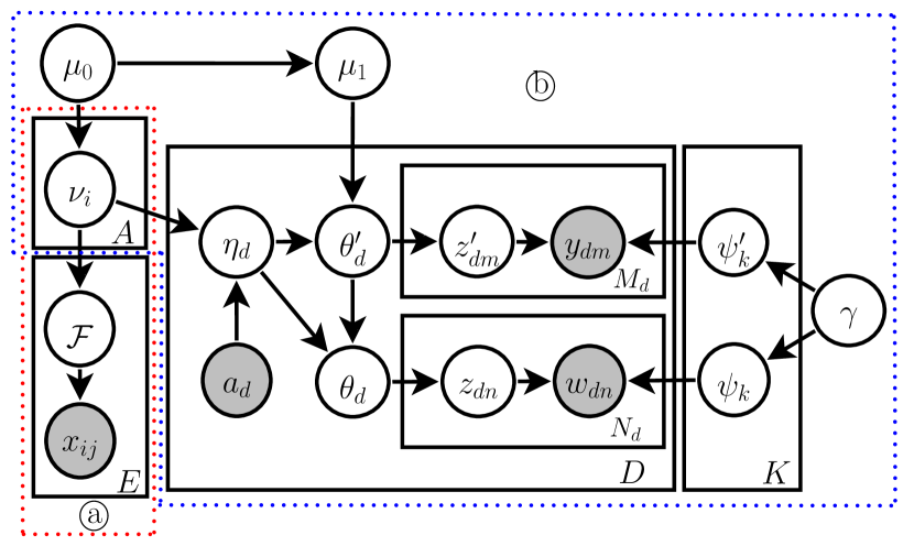
Figure 4: Graphical model for the Twitter-Network Topic Model (TNTM) composed of a HPYP topic model (region ⓑ) and a GP based random function network model (region ⓐ). The author–topic distributions $\nu$ serve to link the two together. Each tweet is modelled with a hierarchy of document–topic distributions denoted by $\eta$, $\theta^{\prime}$, and $\theta$, where each is attuned to the whole tweet, the hashtags, and the words, in that order. With their own topic assignments $z^{\prime}$ and $z$, the hashtags $y$ and the words $w$ are separately modelled. They are generated from the topic–hashtag distributions $\psi^{\prime}$ and the topic–word distributions $\psi$ respectively. The variables $\mu_{0}$ , $\mu_{1}$ and $\gamma$ are priors for the respective PYPs. The connections between the authors are denoted by $x$, modelled by random function $\mathcal{F}$.

The TNTM makes use of the accompanying hashtags, authors, and followers network to model tweets better. The TNTM is composed of two main components: a HPYP topic model for the text and hashtags, and a GP based random function network model for the followers network. The authorship information serves to connect the two together. The HPYP topic model is illustrated by region ⓑ in Figure 4 while the network model is captured by region ⓐ.

5.2.1 HPYP Topic Model

The HPYP topic model described in Section 3 is extended as follows. For the word distributions, we first generate a parent word distribution prior $\gamma$ for all topics:

$$\gamma\sim\mathrm{PYP}(\alpha^{\gamma},\beta^{\gamma},H^{\gamma})\,,$$ (47)

where $H_{\gamma}$ is a discrete uniform distribution over the complete word vocabulary $\mathcal{V}$. Then, we sample the hashtag distribution $\psi^{\prime}_{k}$ and word distribution $\psi_{k}$ for each topic $k$, with $\gamma$ as the base distribution:

$$\psi^{\prime}_{k}\,|\,\gamma \sim\mathrm{PYP}(\alpha^{\psi^{\prime}_{k}},\beta^{\psi^{\prime}_{k}},\gamma)\,,$$ (48)

$$\psi_{k}\,|\,\gamma \sim\mathrm{PYP}(\alpha^{\psi_{k}},\beta^{\psi_{k}},\gamma)\,, \mathrm{for\ \ }k=1,\dots,K\,.$$ (49)

Note that the tokens of the hashtags are shared with the words, that is, the hashtag #happy shares the same token as the word happy, and are thus treated as the same word. This treatment is important since some hashtags are used as words instead of labels. Additionally, this also allows any words to be hashtags, which will be useful for hashtag recommendation.

For the topic distributions, we generate a global topic distribution $\mu_{0}$, which serves as a prior, from a GEM distribution. Then generate the author–topic distribution $\nu_{i}$ for each author $i$, and a miscellaneous topic distribution $\mu_{1}$ to capture topics that deviate from the authors’ usual topics:

$$\mu_{0} \sim\mathrm{GEM}(\alpha^{\mu_{0}},\beta^{\mu_{0}})\,,$$ (50)

$$\mu_{1}\,|\,\mu_{0} \sim\mathrm{PYP}(\alpha^{\mu_{1}},\beta^{\mu_{1}},\mu_{0})\,,$$ (51)

$$\nu_{i}\,|\,\mu_{0} \sim\mathrm{PYP}(\alpha^{\nu_{i}},\beta^{\nu_{i}},\mu_{0})\,, \mathrm{for\ \ }i=1,\dots,A\,.$$ (52)

For each tweet $d$, given the author–topic distribution $\nu$ and the observed author $a_{d}$ , we sample the document–topic distribution $\eta_{d}$ , as follows:

$$\eta_{d}\,|\,a_{d},\nu\sim\mathrm{PYP}(\alpha^{\eta_{d}},\beta^{\eta_{d}},\nu_{a_{d}})\,, \mathrm{for\ \ }d=1,\dots,D\,.$$ (53)

Next, we generate the topic distributions for the observed hashtags ($\theta^{\prime}_{d}$) and the observed words ($\theta_{d}$), following the technique used in the adaptive topic model (Du et al., 2012a). We explicitly model the influence of hashtags to words, by generating the words conditioned on the hashtags. The intuition comes from hashtags being the themes of a tweet, and they drive the content of the tweet. Specifically, we sample the mixing proportions $\rho^{\theta^{\prime}_{d}}$, which control the contribution of $\eta_{d}$ and $\mu_{1}$ for the base distribution of $\theta^{\prime}_{d}$ , and then generate $\theta^{\prime}_{d}$ given $\rho^{\theta^{\prime}_{d}}$:

$$\rho^{\theta^{\prime}_{d}} \sim\mathrm{Beta}\Big{(}\lambda^{\theta^{\prime}_{d}}_{0},\lambda^{\theta^{\prime}_{d}}_{1}\Big{)}\,,$$ (54)

$$\theta^{\prime}_{d}\,|\,\mu_{1},\eta_{d} \sim\mathrm{PYP}\Big{(}\alpha^{\theta^{\prime}_{d}},\beta^{\theta^{\prime}_{d}},\rho^{\theta^{\prime}_{d}}\mu_{1}+(1\!-\!\rho^{\theta^{\prime}_{d}})\eta_{d}\Big{)}\,.$$ (55)

We set $\theta^{\prime}_{d}$ and $\eta_{d}$ as the parent distributions of $\theta_{d}$ . This flexible configuration allows us to investigate the relationship between $\theta_{d}$ , $\theta^{\prime}_{d}$ and $\eta_{d}$ , that is, we can examine if $\theta_{d}$ is directly determined by $\eta_{d}$ , or through the $\theta^{\prime}_{d}$ . The mixing proportions $\rho^{\theta_{d}}$ and the topic distribution $\theta_{d}$ is generated similarly:

$$\rho^{\theta_{d}} \sim\mathrm{Beta}\Big{(}\lambda^{\theta_{d}}_{0},\lambda^{\theta_{d}}_{1}\Big{)}\,,$$ (56)

$$\theta_{d}\,|\,\eta_{d},\theta^{\prime}_{d} \sim\mathrm{PYP}\Big{(}\alpha^{\theta_{d}},\beta^{\theta_{d}},\,\rho^{\theta_{d}}\eta_{m}+(1\!-\!\rho^{\theta_{d}})\theta^{\prime}_{d}\Big{)}\,.$$ (57)

The hashtags and words are then generated in a similar fashion to LDA. For the $m$-th hashtag in tweet $d$, we sample a topic $z^{\prime}_{dm}$ and the hashtag $y_{dm}$ by

$$z^{\prime}_{dm}\,|\,\theta^{\prime}_{d} \sim\mathrm{Discrete}\big{(}\theta^{\prime}_{d}\big{)}\,,$$ (58)

$$y_{dm}\,|\,z^{\prime}_{dm},\psi^{\prime} \sim\mathrm{Discrete}\Big{(}\psi^{\prime}_{z^{\prime}_{dm}}\Big{)}\,, \mathrm{for\ \ }m=1,\dots,M_{d}\,,$$ (59)

where $M_{d}$ is the number of seen hashtags in tweet $d$. While for the $n$-th word in tweet $d$, we sample a topic $z_{dn}$ and the word $w_{dn}$ by

$$z_{dn}\,|\,\theta_{d} \sim\mathrm{Discrete}(\theta_{d})\,,$$ (60)

$$w_{dn}\,|\,z_{dn},\psi \sim\mathrm{Discrete}\big{(}\psi_{z_{dn}}\big{)}\,, \mathrm{for\ \ }n=1,\dots,N_{d}\,,$$ (61)

where $N_{d}$ is the number of observed words in tweet $d$. We note that all above $\alpha$, $\beta$ and $\lambda$ are the hyperparameters of the model. We show the importance of the above modelling with ablation studies in Section 5.6. Although the HPYP topic model may seem complex, it is a simple network of PYP nodes since all distributions on the probability vectors are modelled by the PYP.

5.2.2 Random Function Network Model

The network modelling is connected to the HPYP topic model via the author–topic distributions $\nu$, where we treat $\nu$ as inputs to the GP in the network model. The GP, represented by $\mathcal{F}$, determines the link between two authors ($x_{ij}$), which indicates the existence of the social links between author $i$ and author $j$. For each pair of authors, we sample their connections with the following random function network model:

$$Q_{ij}\,|\,\nu \sim\mathcal{F}(\nu_{i},\nu_{j})\,,$$ (62)

$$x_{ij}\,|\,Q_{ij} \sim\mathrm{Bernoulli}\big{(}s(Q_{ij})\big{)}\,, \mathrm{for\ \ }i=1,\dots,A;\ j=1,\dots,A\,,$$ (63)

where $s(\cdot)$ is the sigmoid function:

$$s(t)=\frac{1}{1+e^{-t}}~{}.$$ (64)

By marginalising out $\mathcal{F}$, we can write $\mathbf{Q}\sim\mathrm{GP}(\varsigma,\kappa)$, where $\mathbf{Q}$ is a vectorised collection of $Q_{ij}$ . $\varsigma$ denotes the mean vector and $\kappa$ is the covariance matrix of the GP:

$$\varsigma_{ij} =\mathrm{Sim}(\nu_{i},\nu_{j})\,,$$ (65)

$$\kappa_{ij,i^{\prime}j^{\prime}} =\frac{s^{2}}{2}\exp\!\Bigg{(}\!-\frac{\big{|}\mathrm{Sim}(\nu_{i},\nu_{j})-\mathrm{Sim}(\nu_{i^{\prime}},\nu_{j^{\prime}})\big{|}^{2}}{2l^{2}}\Bigg{)}+\sigma^{2}I(ij=i^{\prime}j^{\prime})\,,$$ (66)

where $s$, $l$ and $\sigma$ are the hyperparameters associated to the kernel. $\mathrm{Sim}(\cdot,\cdot)$ is a similarity function that has a range between $0$ and $1$, here chosen to be cosine similarity due to its ease of computation and popularity.

5.2.3 Relationships with Other Models

The TNTM is related to many existing models after removing certain components of the model. When hashtags and the network components are removed, the TNTM is reduced to a nonparametric variant of the author topic model (ATM). Oppositely, if authorship information is discarded, the TNTM resembles the correspondence LDA (Blei and Jordan, 2003), although it differs in that it allows hashtags and words to be generated from a common vocabulary.

In contrast to existing parametric models, the network model in the TNTM provides possibly the most flexible way of network modelling via a nonparametric Bayesian prior (GP), following Lloyd et al. (2012). Different to Lloyd et al. (2012), we propose a new kernel function that fits our purpose better and achieves significant improvement over the original kernel.

5.3 Representation and Model Likelihood

As with previous sections, we represent the TNTM using the CRP representation discussed in Section 3.2. However, since the PYP variables in the TNTM can have multiple parents, we extend the representation following Du et al. (2012a). The distinction is that we store multiple tables counts for each PYP, to illustrate, $t_{k}^{\mathcal{N}\to\mathcal{P}}$ represents the number of tables in PYP $\mathcal{N}$ serving dish $k$ that are contributed to the customer counts in PYP $\mathcal{P}$, $c_{k}^{\mathcal{P}}$. Similarly, the total table counts that contribute to $\mathcal{P}$ is denoted as $T^{\mathcal{N}\to\mathcal{P}}=\sum_{k}t_{k}^{\mathcal{N}\to\mathcal{P}}$. Note the number of tables in PYP $\mathcal{N}$ is $t_{k}^{\mathcal{N}}=\sum_{\mathcal{P}}t_{k}^{\mathcal{N}\to\mathcal{P}}$, while the total number of tables is $T^{\mathcal{N}}=\sum_{\mathcal{P}}T^{\mathcal{N}\to\mathcal{P}}$. We refer the readers to Lim et al. (2013, Appendix B) for a detailed discussion.

We use bold face capital letters to denote the set of all relevant lower case variables, for example, we denote $\mathbf{W}^{\circ}=\{\mathbf{W},\mathbf{Y}\}$ as the set of all words and hashtags; $\mathbf{Z}^{\circ}=\{\mathbf{Z},\mathbf{Z}^{\prime}\}$ as the set of all topic assignments for the words and the hashtags; $\mathbf{T}$ as the set of all table counts and $\mathbf{C}$ as the set of all customer counts; and we introduce $\mathbf{\Xi}$ as the set of all hyperparameters. By marginalising out the latent variables, we write down the model likelihood corresponding to the HPYP topic model in terms of the counts:

$$p(\mathbf{Z}^{\circ},\mathbf{T},\mathbf{C}\,|\,\mathbf{W}^{\circ},\mathbf{\Xi})\propto \ p(\mathbf{Z}^{\circ},\mathbf{W}^{\circ},\mathbf{T},\mathbf{C}\,|\,\mathbf{\Xi})$$

$$\propto \ f(\mu_{0})f(\mu_{1})\Bigg{(}\prod_{i=1}^{A}f(\nu_{i})\Bigg{)}\Bigg{(}\prod_{k=1}^{K}f(\psi^{\prime}_{k})f(\psi_{k})\Bigg{)}f(\gamma)$$

$$\ \ \ \times\Bigg{(}\prod_{d=1}^{D}f(\eta_{d})f(\theta^{\prime}_{d})f(\theta_{d})g\big{(}\rho^{\theta^{\prime}_{d}}\big{)}g\big{(}\rho^{\theta}_{d}\big{)}\Bigg{)}\prod_{v=1}^{|\mathcal{V}|}\bigg{(}\frac{1}{|\mathcal{V}|}\bigg{)}^{t_{v}^{\gamma}},$$ (67)

where $f(\mathcal{N})$ is the modularised likelihood corresponding to node $\mathcal{N}$, as defined by Equation (18), and $g(\rho)$ is the likelihood corresponding to the probability $\rho$ that controls which parent node to send a customer to, defined as

$$g(\rho^{\mathcal{N}}) =B\Big{(}\lambda^{\mathcal{N}}_{0}+T^{\mathcal{N}\to\mathcal{P}_{0}},\ \lambda^{\mathcal{N}}_{1}+T^{\mathcal{N}\to\mathcal{P}_{1}}\Big{)}\,,$$ (68)

for $\mathcal{N}\sim\mathrm{PYP}\big{(}\alpha^{\mathcal{N}},\beta^{\mathcal{N}},\,\rho^{\mathcal{N}}\mathcal{P}_{0}+(1\!-\!\rho^{\mathcal{N}})\mathcal{P}_{1}\big{)}$. Note that $B(a,b)$ denotes the Beta function that normalises a Dirichlet distribution, defined as follows:

$$B(a,b)=\frac{\Gamma(a)\,\Gamma(b)}{\Gamma(a+b)}~{}.$$ (69)

For the random function network model, the conditional posterior can be derived as

$$p(\mathbf{Q}\,|\,\mathbf{X},\nu,\mathbf{\Xi})\propto \ p(\mathbf{X},\mathbf{Q}\,|\,\nu,\mathbf{\Xi})$$

$$\propto \ \Bigg{(}\prod_{i=1}^{A}\prod_{j=1}^{A}s(Q_{ij})^{x_{ij}}\,\Big{(}1-s(Q_{ij})\Big{)}^{1-x_{ij}}\Bigg{)}$$

$$\ \ \ \ \ \times|\kappa|^{-\frac{1}{2}}\,\exp\!\bigg{(}\!-\frac{1}{2}(\mathbf{Q}-\varsigma)^{\mathsf{T}}\,\kappa^{-1}\,(\mathbf{Q}-\varsigma)\bigg{)}\,.$$ (70)

The full posterior likelihood is thus the product of the topic model posterior (Equation (67)) and the network posterior (Equation (70)):

$$p(\mathbf{Q},\mathbf{Z}^{\circ},\mathbf{T},\mathbf{C}\,|\,\mathbf{X},\mathbf{W}^{\circ},\mathbf{\Xi})=p(\mathbf{Z}^{\circ},\mathbf{T},\mathbf{C}\,|\,\mathbf{W}^{\circ},\mathbf{\Xi})\,p(\mathbf{Q}\,|\,\mathbf{X},\nu,\mathbf{\Xi})\,.$$ (71)

5.4 Performing Posterior Inference on the TNTM

In the TNTM, combining a GP with a HPYP makes its posterior inference non-trivial. Hence, we employ approximate inference by alternatively performing MCMC sampling on the HPYP topic model and the network model, conditioned on each other. For the HPYP topic model, we employ the flexible framework discussed in Section 3 to perform collapsed blocked Gibbs sampling. For the network model, we derive a Metropolis-Hastings (MH) algorithm based on the elliptical slice sampler (Murray et al., 2010). In addition, the author–topic distributions $\nu$ connecting the HPYP and the GP are sampled with an MH scheme since their posteriors do not follow a standard form. We note that the PYPs in this section can have multiple parents, so we extend the framework in Section 3 to allow for this.

The collapsed Gibbs sampling for the HPYP topic model in TNTM is similar to the procedure in Section 4, although there are two main differences. The first difference is that we need to sample the topics for both words and hashtags, each with a different conditional posterior compared to that of Section 4. While the second is due to the PYPs in TNTM can have multiple parents, thus an alternative to decrementing the counts is required. A detailed discussion on performing posterior inference and hyperparameter sampling is presented in the appendix.

5.5 Twitter Data

For evaluation of the TNTM, we construct a tweet corpus from the Twitter 7 dataset (Yang and Leskovec, 2011), This corpus is queried using the hashtags #sport, #music, #finance, #politics, #science and #tech, chosen for diversity. We remove the non-English tweets with langid.py (Lui and Baldwin, 2012). We obtain the data on the followers network from Kwak et al. (2010). However, note that this followers network data is not complete and does not contain information for all authors. Thus we filter out the authors that are not part of the followers network data from the tweet corpus. Additionally, we also remove authors who have written less than fifty tweets from the corpus. We name this corpus T6 since it is queried with six hashtags. It is consists of 240,517 tweets with 150 authors after filtering.

Besides the T6 corpus, we also use the tweet datasets described in Mehrotra et al. (2013). The datasets contains three corpora, each of them is queried with exactly ten query terms. The first corpus, named the Generic Dataset, are queried with generic terms. The second is named the Specific Dataset, which is composed of tweets on specific named entities. Lastly, the Events Dataset is associated with certain events. The datasets are mainly used for comparing the performance of the TNTM against the tweet pooling techniques in Mehrotra et al. (2013). We present a summary of the tweet corpora in Table 3.

Table 3: Summary of the datasets used in this section, showing the number of tweets ($D$), authors ($A$), unique word tokens ($|\mathcal{V}|$), and the average number of words and hashtags in each tweet. The T6 dataset is queried with six different hashtags and thus has a higher number of hashtags per tweet. We note that there is a typo on the number of tweets for the Events Dataset in Mehrotra et al. (2013), the correct number is 107,128.

Dataset	Tweets	Authors	Vocabulary	Words/Tweet	Hashtags/Tweet
T6	$240\,517$	$150$	$5\,343$	$6.35$	$1.34$
Generic	$359\,478$	$213\,488$	$14\,581$	$6.84$	$0.10$
Specific	$214\,580$	$116\,685$	$15\,751$	$6.31$	$0.25$
Events	$107\,128$	$67\,388$	$12\,765$	$5.84$	$0.17$

5.6 Experiments and Results

We consider several tasks to evaluate the TNTM. The first task involves comparing the TNTM with existing baselines on performing topic modelling on tweets. We also compare the TNTM with the random function network model on modelling the followers network. Next, we evaluate the TNTM with ablation studies, in which we perform comparison with the TNTM itself but with each component taken away. Additionally, we evaluate the clustering performance of the TNTM, we compare the TNTM against the state-of-the-art tweets-pooling LDA method in Mehrotra et al. (2013).

5.6.1 Experiment Settings

In all the following experiments, we vary the discount parameters $\alpha$ for the topic distributions $\mu_{0}$ , $\mu_{1}$ , $\nu_{i}$ , $\eta_{m}$ , $\theta^{\prime}_{m}$ , and $\theta_{m}$ , we set $\alpha$ to $0.7$ for the word distributions $\psi$, $\phi^{\prime}$ and $\gamma$ to induce power-law behaviour (Goldwater et al., 2011). We initialise the concentration parameters $\beta$ to $0.5$, noting that they are learned automatically during inference, we set their hyperprior to $\mathrm{Gamma}(0.1,0.1)$ for a vague prior. We fix the hyperparameters $\lambda$, $s$, $l$ and $\sigma$ to $1$, as we find that their values have no significant impact on the model performance.

In the following evaluations, we run the full inference algorithm for 2,000 iterations for the models to converge. We note that the MH algorithm only starts after 1,000 iterations. We repeat each experiment five times to reduce the estimation error for the evaluations.

5.6.2 Goodness-of-fit Test

Table 4: Test perplexity and network log likelihood comparisons between the HDP-LDA, the nonparametric ATM, the random function network model and the TNTM. Lower perplexity indicates better model fitting. The TNTM significantly outperforms the other models in term of model fitting.

Model	Test Perplexity		Network Log	Likelihood
HDP-LDA	$840.03$ $\pm$	$15.7$	N/A
Nonparametric ATM	$664.25$ $\pm$	$17.76$	N/A
Random Function	N/A		$-557.86$ $\pm$	$11.2$
TNTM	${\bf 505.01}$ $\pm$	$7.8$	${\bf-500.63}$ $\pm$	$13.6$

We compare the TNTM with the HDP-LDA and a nonparametric author-topic model (ATM) on fitting the text data (words and hashtags). Their performances are measured using perplexity on the test set (see Section 4.5.2). The perplexity for the TNTM, accounting for both words and hashtags, is

$$\mathrm{Perplexity}(\mathbf{W}^{\circ})=\exp\!\Bigg{(}-\frac{\log p\big{(}\mathbf{W}^{\circ}\,|\,\nu,\mu_{1},\psi,\psi^{\prime}\big{)}}{\sum_{d=1}^{D}N_{d}+M_{d}}\Bigg{)}\,,$$ (72)

where the likelihood $p\big{(}\mathbf{W}^{\circ}\,|\,\nu,\mu_{1},\psi,\psi^{\prime}\big{)}$ is broken into

$$p\big{(}\mathbf{W}^{\circ}\,|\,\nu,\mu_{1},\psi,\psi^{\prime}\big{)}= \ \prod_{d=1}^{D}\prod_{m=1}^{M_{d}}p(y_{dm}\,|\,\nu,\mu_{1},\psi^{\prime})\prod_{n=1}^{N_{d}}p(w_{dn}\,|\,y_{d},\nu,\mu_{1},\psi)\,.$$ (73)

We also compare the TNTM against the original random function network model in terms of the log likelihood of the network data, given by $\log p(\mathbf{X}\,|\,\nu)$. We present the comparison of the perplexity and the network log likelihood in Table 5.6.2. We note that for the network log likelihood, the less negative the better. From the result, we can see that the TNTM achieves a much lower perplexity compared to the HDP-LDA and the nonparametric ATM. Also, the nonparametric ATM is significantly better than the HDP-LDA. This clearly shows that using more auxiliary information gives a better model fitting. Additionally, we can also see that jointly modelling the text and network data leads to a better modelling on the followers network.

5.6.3 Ablation Test

Table 5: Ablation test on the TNTM. The test perplexity and the network log likelihood is evaluated on the TNTM against several ablated variants of the TNTM. The result shows that each component in the TNTM is important.

TNTM Model	Test Perplexity		Network Log	Likelihood
No author	$669.12$ $\pm$	$9.3$	N/A
No hashtag	$1017.23$ $\pm$	$27.5$	$-522.83$ $\pm$	$17.7$
No $\mu_{1}$ node	$607.70$ $\pm$	$10.7$	$-508.59$ $\pm$	$9.8$
No $\theta^{\prime}$- $\theta$ connection	$551.78$ $\pm$	$16.0$	$-509.21$ $\pm$	$18.7$
No power-law	$508.64$ $\pm$	$7.1$	$-560.28$ $\pm$	$30.7$
Full model	${\bf 505.01}$ $\pm$	$7.8$	${\bf-500.63}$ $\pm$	$13.6$

Next, we perform an extensive ablation study with the TNTM. The components that are tested in this study are (1) authorship, (2) hashtags, (3) PYP $\mu_{1}$ , (4) connection between PYP $\theta^{\prime}_{d}$ and $\theta_{d}$ , and (5) power-law behaviour on the PYPs. We compare the full TNTM against variations in which each component is ablated. Table 5.6.3 presents the test set perplexity and the network log likelihood of these models, it shows significant improvements of the TNTM over the ablated models. From this, we see that the greatest improvement on perplexity is from modelling the hashtags, which suggests that the hashtag information is the most important for modelling tweets. Second to the hashtags, the authorship information is very important as well. Even though modelling the power-law behaviour is not that important for perplexity, we see that the improvement on the network log likelihood is best achieved by modelling the power-law. This is because the flexibility enables us to learn the author–topic distributions better, and thus allowing the TNTM to fit the network data better. This also suggests that the authors in the corpus tend to focus on a specific topic rather than having a wide interest.

5.6.4 Document Clustering and Topic Coherence

Table 6: Clustering evaluations of the TNTM against the LDA with different pooling schemes. Note that higher purity and NMI indicate better performance. The results for the different pooling methods are obtained from Table 4 in Mehrotra et al. (2013). The TNTM achieves better performance on the purity and the NMI for all datasets except for the Specific dataset, where it obtains the same purity score as the best pooling method.

Method/Model	Purity			NMI
Data	Generic	Specific	Events	Generic	Specific	Events
No pooling	$0.49$	$0.64$	$0.69$	$0.28$	$0.22$	$0.39$
Author	$0.54$	$0.62$	$0.60$	$0.24$	$0.17$	$0.41$
Hourly	$0.45$	$0.61$	$0.61$	$0.07$	$0.09$	$0.32$
Burstwise	$0.42$	$0.60$	$0.64$	$0.18$	$0.16$	$0.33$
Hashtag	$0.54$	$\mathbf{0.68}$	$0.71$	$0.28$	$0.23$	$0.42$
TNTM	$\mathbf{0.66}$	$\mathbf{0.68}$	$\mathbf{0.79}$	$\mathbf{0.43}$	$\mathbf{0.31}$	$\mathbf{0.52}$

Mehrotra et al. (2013) shows that running LDA on pooled tweets rather than unpooled tweets gives significant improvement on clustering. In particular, they find that grouping tweets based on the hashtags provides most improvement. Here, we show that instead of resorting to such an ad hoc method, the TNTM can achieve a significantly better result on clustering. The clustering evaluations are measured with purity and normalised mutual information (NMI, see Manning et al., 2008) described in 4.5.3. Since ground truth labels are unknown, we use the respective query terms as the ground truth for evaluations. Note that tweets that satisfy multiple labels are removed. Given the learned model, we assign a tweet to a cluster based on its dominant topic.

We perform the evaluations on the Generic, Specific and Events datasets for comparison purpose. We note the lack of network information in these datasets, and thus we employ only the HPYP part of the TNTM. Additionally, since the purity can trivially be improved by increasing the number of clusters, we limit the maximum number of topics to twenty for a fair comparison. We present the results in Table 5.6.4. We can see that the TNTM outperforms the pooling method in all aspects except on the Specific dataset, where it achieves the same purity as the best pooling scheme.

5.6.5 Automatic Topic Labelling

Traditionally, researchers assign a topic for each topic–word distribution manually by inspection. More recently, there have been attempts to label topics automatically in topic modelling. For instance, Lau et al. (2011) use Wikipedia to extract labels for topics, and Mehdad et al. (2013) use the entailment relations to select relevant phrases for topics. Here, we show that we can use hashtags to obtain good topic labels. In Table 5.6.5, we display the top words from the topic–word distribution $\psi_{k}$ for each topic $k$. Instead of manually assigning the topic labels, we display the top three hashtags from the topic–hashtag distribution $\psi^{\prime}_{k}$ . As we can see from Table 5.6.5, the hashtags appear suitable as topic labels. In fact, by empirically evaluating the suitability of the hashtags in representing the topics, we consistently find that, over 90 % of the hashtags are good candidates for the topic labels. Moreover, inspecting the topics show that the major hashtags coincide with the query terms used in constructing the T6 dataset, which is to be expected. This verifies that the TNTM is working properly.

Table 7: Topical analysis on the T6 dataset with the TNTM, which displays the top three hashtags and the top $n$ words on six topics. Instead of manually assigning a topic label to the topics, we find that the top hashtags can serve as the topic labels.

Topic	Top Hashtags	Top Words
Topic 1	finance, money, economy	finance, money, bank, marketwatch,
		stocks, china, group, shares, sales
Topic 2	politics, iranelection, tcot	politics, iran, iranelection, tcot,
		tlot, topprog, obama, musiceanewsfeed
Topic 3	music, folk, pop	music, folk, monster, head, pop,
		free, indie, album, gratuit, dernier
Topic 4	sports, women, asheville	sports, women, football, win, game,
		top, world, asheville, vols, team
Topic 5	tech, news, jobs	tech, news, jquery, jobs, hiring,
		gizmos, google, reuters
Topic 6	science, news, biology	science, news, source, study, scientists,
		cancer, researchers, brain, biology, health

6 Conclusion

In this article, we proposed a topic modelling framework utilising PYPs, for which their realisation is a probability distribution or another stochastic process of the same type. In particular, for the purpose of performing inference, we described the CRP representation for the PYPs. This allows us to propose a single framework, discussed in Section 3, to implement these topic models, where we modularise the PYPs (and other variables) into blocks that can be combined to form different models. Doing so enables significant time to be saved on implementation of the topic models.

We presented a general HPYP topic model, that can be seen as a generalisation to the HDP-LDA (Teh and Jordan, 2010). The HPYP topic model is represented using a Chinese Restaurant Process (CRP) metaphor (Teh and Jordan, 2010; Blei et al., 2010; Chen et al., 2011), and we discussed how the posterior likelihood of the HPYP topic model can be modularised. We then detailed the learning algorithm for the topic model in the modularised form.

We applied our HPYP topic model framework on Twitter data and proposed the Twitter-Network Topic model (TNTM). The TNTM models the authors, text, hashtags, and the authors-follower network in an integrated manner. In addition to HPYP, the TNTM employs the Gaussian process (GP) for the network modelling. The main suggested use of the TNTM is for content discovery on social networks. Through experiments, we show that jointly modelling of the text content and the network leads to better model fitting as compared to modelling them separately. Results on the qualitative analysis show that the learned topics and the authors’ topics are sound. Our experiments suggest that incorporating more auxiliary information leads to better fitting models.

6.1 Future Research

For future work on TNTM, it would be interesting to apply TNTM to other types of data, such as blogs and news feeds. We could also use TNTM for other applications. such as hashtag recommendation and content suggestion for new Twitter users. Moreover, we could extend TNTM to incorporate more auxiliary information: for instance, we can model the location of tweets and the embedded multimedia contents such as URL, images and videos. Another interesting source of information would be the path of retweeted content.

Another interesting area of research is the combination of different kinds of topic models for a better analysis. This allows us to transfer learned knowledge from one topic model to another. The work on combining LDA has already been looked at by Schnober and Gurevych (2015), however, combining other kinds of topic models, such as nonparametric ones, is unexplored.

Acknowledgments

The authors like to thank Shamin Kinathil, the editors, and the anonymous reviewers for their valuable feedback and comments. NICTA is funded by the Australian Government through the Department of Communications and the Australian Research Council through the ICT Centre of Excellence Program.

A Posterior Inference for TNTM

A.1 Decrementing the Counts Associated with a Word or Hashtag

When we remove a word or a hashtag during inference, we decrement by one the customer count from the PYP associated with the word or the hashtag, that is, $c_{k}^{\theta_{d}}$ for word $w_{dn}$ ($z_{dn}=k$) and $c_{k}^{\theta^{\prime}_{d}}$ for hashtag $y_{dm}$ ($z^{\prime}_{dm}=k$). Decrementing the customer count may or may not decrement the respective table count. However, if the table count is decremented, then we would decrement the customer count of the parent PYP. This is relatively straight forward in Section 4.1 since the PYPs have only one parent. Here, when a PYP $\mathcal{N}$ has multiple parents, we would sample for one of its parent PYPs and decrement the table count corresponding to the parent PYP. Although not the same, the rationale of this procedure follows Section 4.1.

We explain in more details below. When the customer count $c_{k}^{\mathcal{N}}$ is decremented, we introduce an auxiliary variable $u_{k}^{\mathcal{N}}$ that indicates which parent of $\mathcal{N}$ to remove a table from, or none at all. The sample space for $u_{k}^{\mathcal{N}}$ is the $P$ parent nodes $\mathcal{P}_{1}\,,\dots,\mathcal{P}_{P}$ of $\mathcal{N}$, plus $\emptyset$. When $u_{k}^{\mathcal{N}}$ is equal to $\mathcal{P}_{i}$ , we decrement the table count $t_{k}^{\mathcal{N}\to\mathcal{P}_{i}}$ and subsequently decrement the customer count $c_{k}^{\mathcal{P}_{i}}$ in node $\mathcal{P}_{i}$ . If $u_{k}^{\mathcal{N}}$ equals to $\emptyset$, we do not decrement any table count. The process is repeated recursively as long as a customer count is decremented, that is, we stop when $u^{\mathcal{N}}_{k}=\emptyset$.

The value of $u^{\mathcal{N}}_{k}$ is sampled as follows:

$$p\big{(}u^{\mathcal{N}}_{k}\big{)}=\left\{\begin{array}[]{ll}t^{\mathcal{N}\to\mathcal{P}_{i}}_{k}/c^{\mathcal{N}}_{k}&~{}~{}\mathrm{if~{}~{}}u^{\mathcal{N}}_{k}=\mathcal{P}_{i}\\[6.0pt] 1-\sum_{\mathcal{P}_{i}}p\big{(}u^{\mathcal{N}}_{k}=\mathcal{P}_{i}\big{)}&~{}~{}\mathrm{if~{}~{}}u^{\mathcal{N}}_{k}=\emptyset~{}~{}.\end{array}\right.$$ (74)

To illustrate, when a word $w_{dn}$ (with topic $z_{dn}$) is removed, we decrement $c^{\theta_{d}}_{z_{dn}}$ , that is, $c^{\theta_{d}}_{z_{dn}}$ becomes $c^{\theta_{d}}_{z_{dn}}-1$. We then determine if this word contributes to any table in node $\theta_{d}$ by sampling $u^{\theta_{d}}_{z_{dn}}$ from Equation (74). If $u^{\theta_{d}}_{z_{dn}}=\emptyset$, we do not decrement any table count and proceed with the next step in Gibbs sampling; otherwise, $u^{\theta_{d}}_{z_{dn}}$ can either be $\theta^{\prime}_{d}$ or $\eta_{d}$ , in these cases, we would decrement $t^{\theta_{d}\to u^{\theta_{d}}_{z_{dn}}}_{z_{dn}}$ and $c^{u^{\theta_{d}}_{z_{dn}}}_{z_{dn}}$, and continue the process recursively.

We present the decrementing process in Algorithm 2. To remove a word $w_{dn}$ during inference, we would need to decrement the counts contributed by $w_{dn}$ (and $z_{dn}$). For the topic side, we decrement the counts associated with node $\mathcal{N}=\theta_{d}$ with group $k=z_{dn}$ using Algorithm 2. While for the vocabulary side, we decrement the counts associated with the node $\mathcal{N}=\psi_{z_{dn}}$ with group $k=w_{dn}$ . The effect of the word on the other PYP variables are implicitly considered through recursion.

Note that the procedure to decrementing a hashtag $y_{dm}$ is similar, in this case, we decrement the counts for $\mathcal{N}=\theta^{\prime}_{d}$ with $k=z^{\prime}_{dm}$ (topic side), then decrement the counts for $\mathcal{N}=\psi^{\prime}_{z^{\prime}_{dm}}$ with $k=y_{dm}$ (vocabulary side).

Algorithm 2 Decrementing counts associated with a PYP $\mathcal{N}$ and group $k$.

1. Decrement the customer count $c_{k}^{\mathcal{N}}$ by one.

2. Sample an auxiliary variable $u_{k}^{\mathcal{N}}$ with Equation (74).

3. For the sampled $u_{k}^{\mathcal{N}}$, perform the following:

   1. If $u_{k}^{\mathcal{N}}=\emptyset$, exit the algorithm.

   2. Otherwise, decrement the table count $t_{k}^{\mathcal{N}\to u_{k}^{\mathcal{N}}}$ by one and repeat Steps 2 – 4 by replacing $\mathcal{N}$ with $u_{k}^{\mathcal{N}}$.

A.2 Sampling a New Topic for a Word or a Hashtag

After decrementing, we sample a new topic for the word or the hashtag. The sampling process follows the procedure discussed in Section 4.2, but with different conditional posteriors (for both the word and the hashtag). The full conditional posterior probability for the collapsed blocked Gibbs sampling can be derived easily. For instance, the conditional posterior for sampling the topic $z_{dn}$ of word $w_{dn}$ is

$$p(z_{dn},\mathbf{T},\mathbf{C}\,|\,{\mathbf{Z}^{\circ}}^{-dn},\mathbf{W}^{\circ},\mathbf{T}^{-dn},\mathbf{C}^{-dn},\mathbf{\Xi})=\frac{p(\mathbf{Z}^{\circ},\mathbf{T},\mathbf{C}\,|\,\mathbf{W}^{\circ},\mathbf{\Xi})}{p({\mathbf{Z}^{\circ}}^{-dn},\mathbf{T}^{-dn},\mathbf{C}^{-dn}\,|\,\mathbf{W}^{\circ},\mathbf{\Xi})}$$ (75)

which can then be easily decomposed into simpler form (see discussion in Section 4.2) using Equation (67). Here, the superscript $\Box^{-dn}$ indicates the word $w_{dn}$ and the topic $z_{dn}$ are removed from the respective sets. Similarly, the conditional posterior probability for sampling the topic $z^{\prime}_{dm}$ of hashtag $y_{dm}$ can be derived as

$$p(z^{\prime}_{dm},\mathbf{T},\mathbf{C}\,|\,{\mathbf{Z}^{\circ}}^{-dm},\mathbf{W}^{\circ},\mathbf{T}^{-dm},\mathbf{C}^{-dm},\mathbf{\Xi})=\frac{p(\mathbf{Z}^{\circ},\mathbf{T},\mathbf{C}\,|\,\mathbf{W}^{\circ},\mathbf{\Xi})}{p({\mathbf{Z}^{\circ}}^{-dm},\mathbf{T}^{-dm},\mathbf{C}^{-dm}\,|\,\mathbf{W}^{\circ},\mathbf{\Xi})}$$ (76)

where the superscript $\Box^{-dm}$ signals the removal of the hashtag $y_{dm}$ and the topic $z^{\prime}_{dm}$ . As in Section 4.2, we compute the posterior for all possible changes to $\mathbf{T}$ and $\mathbf{C}$ corresponding to the new topic (for $z_{dn}$ or $z^{\prime}_{dm}$). We then sample the next state using a Gibbs sampler.

A.3 Estimating the Probability Vectors of the PYPs with Multiple Parents

Following Section 4.4, we estimate the various probability distributions of the PYPs by their posterior means. For a PYP $\mathcal{N}$ with a single PYP parent $\mathcal{P}_{1}$ , as discussed in Section 4.4, we can estimate its probability vector $\hat{\mathcal{N}}=(\hat{\mathcal{N}}_{1},\dots,\hat{\mathcal{N}}_{K})$ as

$$\hat{\mathcal{N}}_{k} =\mathbb{E}[\mathcal{N}_{k}\,|\,\mathbf{Z}^{\circ},\mathbf{W}^{\circ},\mathbf{T},\mathbf{C},\mathbf{\Xi}]$$

$$=\frac{\big{(}\alpha^{\mathcal{N}}T^{\mathcal{N}}+\beta^{\mathcal{N}}\big{)}\mathbb{E}[\mathcal{P}_{1k}\,|\,\mathbf{Z}^{\circ},\mathbf{W}^{\circ},\mathbf{T},\mathbf{C},\mathbf{\Xi}]+c_{k}^{\mathcal{N}}-\alpha^{\mathcal{N}}T_{k}^{\mathcal{N}}}{\beta^{\mathcal{N}}+C^{\mathcal{N}}}~{},$$ (77)

which lets one analyse the probability vectors in a topic model using recursion.

Unlike the above, the posterior mean is slightly more complicated for a PYP $\mathcal{N}$ that has multiple PYP parents $\mathcal{P}_{1},\dots,\mathcal{P}_{P}$ . Formally, we define the PYP $\mathcal{N}$ as

$$\mathcal{N}\,|\,\mathcal{P}_{1},\dots,\mathcal{P}_{P}\sim\mathrm{PYP}\Big{(}\alpha^{\mathcal{N}},\beta^{\mathcal{N}},\rho_{1}^{\mathcal{N}}\mathcal{P}_{1}+\dots+\rho_{P}^{\mathcal{N}}\mathcal{P}_{P}\Big{)}\,,$$ (78)

where the mixing proportion $\rho^{\mathcal{N}}=(\rho_{1}^{\mathcal{N}},\dots,\rho_{P}^{\mathcal{N}})$ follows a Dirichlet distribution with parameter $\lambda^{\mathcal{N}}=(\lambda_{1}^{\mathcal{N}},\dots,\lambda_{P}^{\mathcal{N}})$:

$$\rho^{\mathcal{N}} \sim\mathrm{Dirichlet}\big{(}\lambda^{\mathcal{N}}\big{)}\,.$$ (79)

Before we can estimate the probability vector, we first estimate the mixing proportion with its posterior mean given the customer counts and table counts:

$$\hat{\rho}_{i}^{\mathcal{N}}=\mathbb{E}[\rho_{i}^{\mathcal{N}}\,|\,\mathbf{Z}^{\circ},\mathbf{W}^{\circ},\mathbf{T},\mathbf{C},\mathbf{\Xi}]=\frac{T^{\mathcal{N}\to\mathcal{P}_{i}}+\lambda_{i}^{\mathcal{N}}}{T^{\mathcal{N}}+\sum_{i}\lambda_{i}^{\mathcal{N}}}~{}.$$ (80)

Then, we can estimate the probability vector $\hat{\mathcal{N}}=(\hat{\mathcal{N}}_{1},\dots,\hat{\mathcal{N}}_{K})$ by

$$\hat{\mathcal{N}}_{k} =\frac{\big{(}\alpha^{\mathcal{N}}T^{\mathcal{N}}+\beta^{\mathcal{N}}\big{)}\hat{H}_{k}^{\mathcal{N}}+c_{k}^{\mathcal{N}}-\alpha^{\mathcal{N}}T_{k}^{\mathcal{N}}}{\beta^{\mathcal{N}}+C^{\mathcal{N}}}~{},$$ (81)

where $\hat{H}^{\mathcal{N}}=(\hat{H}_{1}^{\mathcal{N}},\dots,\hat{H}_{K}^{\mathcal{N}})$ is the expected base distribution:

$$\hat{H}_{k}^{\mathcal{N}}=\sum_{i=1}^{P}\hat{\rho}_{i}^{\mathcal{N}}\mathbb{E}[\mathcal{P}_{ik}\,|\,\mathbf{Z}^{\circ},\mathbf{W}^{\circ},\mathbf{T},\mathbf{C},\mathbf{\Xi}]\,.$$ (82)

With these formulations, all the topic distributions and the word distributions in the TNTM can be reconstructed from the customer counts and table counts. For instance, the author–topic distribution $\nu_{i}$ of each author $i$ can be determined recursively by first estimating the topic distribution $\mu_{0}$ . The word distributions for each topic are similarly estimated.

A.4 MH Algorithm for the Random Function Network Model

Here, we discuss how we learn the topic distributions $\mu_{0}$ and $\nu$ from the random function network model. We configure the MH algorithm to start after running one thousand iterations of the collapsed blocked Gibbs sampler, this is to we can quickly initialise the TNTM with the HPYP topic model before running the full algorithm. In addition, this allows us to demonstrate the improvement to the TNTM due to the random function network model.

To facilitate the MH algorithm, we have to represent the topic distributions $\mu_{0}$ and $\nu$ explicitly as probability vectors, that is, we do not store the customer counts and table counts for $\mu_{0}$ and $\nu$ after starting the MH algorithm. In the MH algorithm, we propose new samples for $\mu_{0}$ and $\nu$, and then accept or reject the samples. The details for the MH algorithm is as follow.

In each iteration of the MH algorithm, we use the Dirichlet distributions as proposal distributions for $\mu_{0}$ and $\nu$:

$$q(\mu_{0}^{\mathrm{new}}\,|\,\mu_{0}) =\mathrm{Dirichlet}(\beta^{\mu_{0}}\mu_{0})\,,$$ (83)

$$q(\nu_{i}^{\mathrm{new}}\,|\,\nu_{i}) =\mathrm{Dirichlet}(\beta^{\nu_{i}}\nu_{i})\,.$$ (84)

These proposed $\mu_{0}$ and $\nu$ are sampled given the their previous values, and we note that the first $\mu_{0}$ and $\nu$ are computed using the technique discussed in A.3. These proposed samples are subsequently used to sample $\mathbf{Q}^{\mathrm{new}}$. We first compute the quantities $\varsigma^{\mathrm{new}}$ and $\kappa^{\mathrm{new}}$ using the proposed $\mu_{0}^{\mathrm{new}}$ and $\nu^{\mathrm{new}}$ with Equation (65) and Equation (66). Then we sample $\mathbf{Q}^{\mathrm{new}}$ given $\varsigma^{\mathrm{new}}$ and $\kappa^{\mathrm{new}}$ using the elliptical slice sampler (see Murray et al., 2010):

$$\mathbf{Q}^{\mathrm{new}}\sim\mathrm{GP}(\varsigma^{\mathrm{new}},\kappa^{\mathrm{new}})\,.$$ (85)

Finally, we compute the acceptance probability $A^{\prime}=\min(A,1)$, where

$$A= \ \frac{p(\mathbf{Q}^{\mathrm{new}}\,|\,\mathbf{X},\nu^{\mathrm{new}},\mathbf{\Xi})}{p(\mathbf{Q}^{\mathrm{old}}\,|\,\mathbf{X},\nu^{\mathrm{old}},\mathbf{\Xi})}\frac{f^{*}(\mu_{0}^{\mathrm{new}}\,|\,\nu^{\mathrm{new}},\mathbf{T})\,\prod_{i=1}^{A}f^{*}(\nu_{i}^{\mathrm{new}}\,|\,\mathbf{T})}{f^{*}(\mu_{0}^{\mathrm{old}}\,|\,\nu^{\mathrm{old}},\mathbf{T})\,\prod_{i=1}^{A}f^{*}(\nu_{i}^{\mathrm{old}}\,|\,\mathbf{T})}$$

$$\ \ \ \ \times\frac{q(\mu_{0}^{\mathrm{old}}\,|\,\mu_{0}^{\mathrm{new}})\,\prod_{i=1}^{A}q(\nu_{i}^{\mathrm{old}}\,|\,\nu_{i}^{\mathrm{new}})}{q(\mu_{0}^{\mathrm{new}}\,|\,\mu_{0}^{\mathrm{old}})\,\prod_{i=1}^{A}q(\nu_{i}^{\mathrm{new}}\,|\,\nu_{i}^{\mathrm{old}})}~{},$$ (86)

and we define $f^{*}(\mu_{0}\,|\,\nu,\mathbf{T})$ and $f^{*}(\nu\,|\,\mathbf{T})$ as

$$f^{*}(\mu_{0}\,|\,\nu,\mathbf{T}) =\prod_{k=1}^{K}(\mu_{0k})^{t_{k}^{\mu_{1}}+\sum_{i=1}^{A}\nu_{i}}~{},$$ (87)

$$f^{*}(\nu_{i}\,|\,\mathbf{T}) =\prod_{k=1}^{K}(\nu_{ik})^{\sum_{d=1}^{D}t_{k}^{\eta_{d}}I(a_{d}=i)}~{}.$$ (88)

The $f^{*}(\cdot)$ corresponds to the topic model posterior of the variables $\mu_{0}$ and $\nu$ after we represent them as probability vectors explicitly. Note that we treat the acceptance probability $A$ as $1$ when the expression in Equation (86) evaluates to more than $1$. We then accept the proposed samples with probability $A$, if the sample are not accepted, we keep the respective old values. This completes one iteration of the MH scheme. We summarise the MH algorithm in Algorithm 3.

Algorithm 3 Performing the MH algorithm for one iteration.

1. Propose a new $\mu_{0}^{\mathrm{new}}$ with Equation (83).

2. For each author $i$, propose a new $\nu_{i}^{\mathrm{new}}$ with Equation (84).

3. Compute the mean function $\varsigma^{\mathrm{new}}$ and the covariance matrix $\kappa^{\mathrm{new}}$ with Equation (65) and Equation (66).

4. Sample $\mathbf{Q}^{\mathrm{new}}$ from Equation (85) using the elliptical slice sampler from Murray et al. (2010).

5. Accept or reject the samples with acceptance probability from Equation (86).

A.5 Hyperparameter Sampling

We sample the hyperparameters $\beta$ using an auxiliary variable sampler while leaving $\alpha$ fixed. We note that the auxiliary variable sampler for PYPs that have multiple parents are identical to that of PYPs with single parent, since the sampler only used the total customer counts $C^{\mathcal{N}}$ and the total table counts $T^{\mathcal{N}}$ for a PYP $\mathcal{N}$. We refer the readers to Section 4.3 for details.

We would like to point out that hyperparameter sampling is performed for all PYPs in TNTM for the first one thousand iterations. After that, as $\mu_{0}$ and $\nu$ are represented as probability vectors explicitly, we only sample the hyperparameters for the other PYPs (except $\mu_{0}$ and $\nu$). We note that sampling the concentration parameters allows the topic distributions of each author to vary, that is, some authors have few very specific topics and some other authors can have a wider range of topics. For simplicity, we fix the kernel hyperparameters $s$, $l$ and $\sigma$ to $1$. Additionally, we also make the priors for the mixing proportions uninformative by setting the $\lambda$ to $1$. We summarise the full inference algorithm for the TNTM in Algorithm 4.

Algorithm 4 Full inference algorithm for the TNTM.

1. Initialise the HPYP topic model by assigning random topic to the latent topic $z_{dn}$ associated with each word $w_{dn}$ , and to the latent topic $z^{\prime}_{dm}$ associated with each hashtag $y_{dm}$ . Then update all the relevant customer counts $\mathbf{C}$ and table counts $\mathbf{T}$.

2. For each word $w_{dn}$ in each document $d$, perform the following:

   1. Decrement the counts associated with $w_{dn}$ (see A.1).

   2. Blocked sample a new topic for $z_{dn}$ and corresponding customer counts $\mathbf{C}$ and table counts $\mathbf{T}$ (with Equation (75)).

   3. Update (increment counts) the topic model based on the sample.

3. For each hashtag $y_{dm}$ in each document $d$, perform the following:

   1. Decrement the counts associated with $y_{dm}$ (see A.1).

   2. Blocked sample a new topic for $z^{\prime}_{dn}$ and corresponding customer counts $\mathbf{C}$ and table counts $\mathbf{T}$ (with Equation (76)).

   3. Update (increment counts) the topic model based on the sample.

4. Sample the hyperparameter $\beta^{\mathcal{N}}$ for each PYP $\mathcal{N}$ (see A.5).

5. Repeat Steps 2 – 4 for 1,000 iterations.

6. Alternatingly perform the MH algorithm (Algorithm 3) and the collapsed blocked Gibbs sampler conditioned on $\mu_{0}$ and $\nu$.

7. Sample the hyperparameter $\beta^{\mathcal{N}}$ for each PYP $\mathcal{N}$ except for $\mu_{0}$ and $\nu$.

8. Repeat Steps 6 – 7 until the model converges or when a fix number of iterations is reached.

References

- Aoki (2008) Aoki, M. (2008). Thermodynamic limits of macroeconomic or financial models: One- and two-parameter Poisson-Dirichlet models. Journal of Economic Dynamics and Control, 32(1):66–84.
- Archambeau et al. (2015) Archambeau, C., Lakshminarayanan, B., and Bouchard, G. (2015). Latent IBP compound Dirichlet allocation. IEEE Transactions on Pattern Analysis and Machine Intelligence, 37(2):321–333.
- Aula (2010) Aula, P. (2010). Social media, reputation risk and ambient publicity management. Strategy & Leadership, 38(6):43–49.
- Baldwin et al. (2013) Baldwin, T., Cook, P., Lui, M., MacKinlay, A., and Wang, L. (2013). How noisy social media text, how diffrnt [sic] social media sources? In Proceedings of the Sixth International Joint Conference on Natural Language Processing, IJCNLP 2013, pages 356–364, Nagoya, Japan. Asian Federation of Natural Language Processing.
- Blei (2012) Blei, D. M. (2012). Probabilistic topic models. Communications of the ACM, 55(4):77–84.
- Blei et al. (2010) Blei, D. M., Griffiths, T. L., and Jordan, M. I. (2010). The nested Chinese Restaurant Process and Bayesian nonparametric inference of topic hierarchies. Journal of the ACM, 57(2):7:1–7:30.
- Blei and Jordan (2003) Blei, D. M. and Jordan, M. I. (2003). Modeling annotated data. In Proceedings of the 26th Annual International ACM SIGIR Conference on Research and Development in Informaion Retrieval, SIGIR 2003, pages 127–134, New York, NY, USA. ACM.
- Blei and Lafferty (2006) Blei, D. M. and Lafferty, J. D. (2006). Dynamic topic models. In Proceedings of the 23rd International Conference on Machine Learning, ICML 2006, pages 113–120, New York, NY, USA. ACM.
- Blei et al. (2003) Blei, D. M., Ng, A. Y., and Jordan, M. I. (2003). Latent Dirichlet Allocation. Journal of Machine Learning Research, 3:993–1022.
- Broersma and Graham (2012) Broersma, M. and Graham, T. (2012). Social media as beat. Journalism Practice, 6(3):403–419.
- Bryant and Sudderth (2012) Bryant, M. and Sudderth, E. B. (2012). Truly nonparametric online variational inference for hierarchical Dirichlet processes. In Advances in Neural Information Processing Systems 25, pages 2699–2707. Curran Associates, Rostrevor, Northern Ireland.
- Buntine and Hutter (2012) Buntine, W. L. and Hutter, M. (2012). A Bayesian view of the Poisson-Dirichlet process. ArXiv e-prints arXiv:1007.0296v2.
- Buntine and Mishra (2014) Buntine, W. L. and Mishra, S. (2014). Experiments with non-parametric topic models. In Proceedings of the 20th ACM SIGKDD International Conference on Knowledge Discovery and Data Mining, KDD 2014, pages 881–890, New York, NY, USA. ACM.
- Canny (2004) Canny, J. (2004). GaP: a factor model for discrete data. In Proceedings of the 27th Annual International ACM SIGIR Conference on Research and Development in Informaion Retrieval, SIGIR 2014, pages 122–129, New York, NY, USA. ACM.
- Chen et al. (2011) Chen, C., Du, L., and Buntine, W. L. (2011). Sampling table configurations for the hierarchical Poisson-Dirichlet process. In Proceedings of the 2011 European Conference on Machine Learning and Knowledge Discovery in Databases - Volume Part I, ECML 2011, pages 296–311, Berlin, Heidelberg. Springer-Verlag.
- Correa et al. (2010) Correa, T., Hinsley, A. W., and de Zúñiga, H. G. (2010). Who interacts on the Web?: The intersection of users’ personality and social media use. Computers in Human Behavior, 26(2):247–253.
- Du (2012) Du, L. (2012). Non-parametric Bayesian methods for structured topic models. PhD thesis, The Australian National University, Canberra, Australia.
- Du et al. (2012a) Du, L., Buntine, W. L., and Jin, H. (2012a). Modelling sequential text with an adaptive topic model. In Proceedings of the 2012 Joint Conference on Empirical Methods in Natural Language Processing and Computational Natural Language Learning, EMNLP-CoNLL 2012, pages 535–545, Stroudsburg, PA, USA. ACL.
- Du et al. (2012b) Du, L., Buntine, W. L., Jin, H., and Chen, C. (2012b). Sequential latent Dirichlet allocation. Knowledge and Information Systems, 31(3):475–503.
- Eisenstein (2013) Eisenstein, J. (2013). What to do about bad language on the internet. In Proceedings of the 2013 Conference of the North American Chapter of the ACL: Human Language Technologies, NAACL-HLT 2013, pages 359–369, Stroudsburg, PA, USA. ACL.
- Erosheva and Fienberg (2005) Erosheva, E. A. and Fienberg, S. E. (2005). Bayesian Mixed Membership Models for Soft Clustering and Classification, pages 11–26. Springer Berlin Heidelberg, Berlin, Heidelberg.
- Favaro et al. (2009) Favaro, S., Lijoi, A., Mena, R. H., and Prünster, I. (2009). Bayesian non-parametric inference for species variety with a two-parameter Poisson-Dirichlet process prior. Journal of the Royal Statistical Society: Series B (Statistical Methodology), 71(5):993–1008.
- Ferguson (1973) Ferguson, T. S. (1973). A Bayesian analysis of some nonparametric problems. The Annals of Statistics, 1(2):209–230.
- Gelman et al. (2013) Gelman, A., Carlin, J. B., Stern, H. S., Dunson, D. B., Vehtari, A., and Rubin, D. B. (2013). Bayesian Data Analysis, Third Edition. Chapman & Hall/CRC Texts in Statistical Science. CRC Press, Boca Raton, FL, USA.
- Geman and Geman (1984) Geman, S. and Geman, D. (1984). Stochastic relaxation, Gibbs distributions, and the Bayesian restoration of images. IEEE Transactions on Pattern Analysis and Machine Intelligence, PAMI-6(6):721–741.
- Goldwater et al. (2005) Goldwater, S., Griffiths, T. L., and Johnson, M. (2005). Interpolating between types and tokens by estimating power-law generators. In Advances in Neural Information Processing Systems 18, NIPS 2005, pages 459–466. MIT Press, Cambridge, MA, USA.
- Goldwater et al. (2011) Goldwater, S., Griffiths, T. L., and Johnson, M. (2011). Producing power-law distributions and damping word frequencies with two-stage language models. Journal of Machine Learning Research, 12:2335–2382.
- Green (1995) Green, P. J. (1995). Reversible jump Markov chain Monte Carlo computation and Bayesian model determination. Biometrika, 82(4):711–732.
- Green and Mira (2001) Green, P. J. and Mira, A. (2001). Delayed rejection in reversible jump Metropolis-Hastings. Biometrika, 88(4):1035–1053.
- Hastings (1970) Hastings, W. K. (1970). Monte Carlo sampling methods using Markov chains and their applications. Biometrika, 57(1):97–109.
- He (2012) He, Y. (2012). Incorporating sentiment prior knowledge for weakly supervised sentiment analysis. ACM Transactions on Asian Language Information Processing (TALIP), 11(2):4:1–4:19.
- Hjort et al. (2010) Hjort, N. L., Holmes, C., Müller, P., and Walker, S. G. (2010). Bayesian Nonparametrics, volume 28. Cambridge University Press, Cambridge, England.
- Hoffman et al. (2013) Hoffman, M. D., Blei, D. M., Wang, C., and Paisley, J. (2013). Stochastic variational inference. Journal of Machine Learning Research, 14:1303–1347.
- Hofmann (1999) Hofmann, T. (1999). Probabilistic latent semantic indexing. In Proceedings of the 22nd Annual International ACM SIGIR Conference on Research and Development in Information Retrieval, SIGIR 1999, pages 50–57, New York, NY, USA. ACM.
- Ishwaran and James (2001) Ishwaran, H. and James, L. F. (2001). Gibbs sampling methods for stick-breaking priors. Journal of the American Statistical Association, 96(453):161–173.
- Jelinek (1997) Jelinek, F. (1997). Statistical Methods for Speech Recognition. MIT Press, Cambridge, MA, USA.
- Jin et al. (2011) Jin, O., Liu, N. N., Zhao, K., Yu, Y., and Yang, Q. (2011). Transferring topical knowledge from auxiliary long texts for short text clustering. In Proceedings of the 20th ACM International Conference on Information and Knowledge Management, CIKM 2011, pages 775–784, New York, NY, USA. ACM.
- Jurafsky and Martin (2000) Jurafsky, D. and Martin, J. H. (2000). Speech & Language Processing. Prentice-Hall, Upper Saddle River, NJ, USA.
- Karimi et al. (2013) Karimi, S., Yin, J., and Paris, C. (2013). Classifying microblogs for disasters. In Proceedings of the 18th Australasian Document Computing Symposium, ADCS 2013, pages 26–33, New York, NY, USA. ACM.
- Kataria et al. (2011) Kataria, S., Mitra, P., Caragea, C., and Giles, C. L. (2011). Context sensitive topic models for author influence in document networks. In Proceedings of the Twenty-Second International Joint Conference on Artificial Intelligence - Volume Three, IJCAI 2011, pages 2274–2280, Palo Alto, CA, USA. AAAI Press.
- Kim et al. (2012) Kim, D., Kim, S., and Oh, A. (2012). Dirichlet process with mixed random measures: A nonparametric topic model for labeled data. In Proceedings of the 29th International Conference on Machine Learning, ICML 2012, pages 727–734, New York, NY, USA. Omnipress.
- Kinsella et al. (2011) Kinsella, S., Murdock, V., and O’Hare, N. (2011). “I’m eating a sandwich in Glasgow”: Modeling locations with tweets. In Proceedings of the 3rd International Workshop on Search and Mining User-generated Contents, SMUC 2011, pages 61–68, New York, NY, USA. ACM.
- Kwak et al. (2010) Kwak, H., Lee, C., Park, H., and Moon, S. (2010). What is Twitter, a social network or a news media? In Proceedings of the 19th International Conference on World Wide Web, WWW 2010, pages 591–600, New York, NY, USA. ACM.
- Landauer et al. (2007) Landauer, T. K., McNamara, D. S., Dennis, S., and Kintsch, W. (2007). Handbook of Latent Semantic Analysis. Lawrence Erlbaum, Mahwah, NJ, USA.
- Lau et al. (2011) Lau, J. H., Grieser, K., Newman, D., and Baldwin, T. (2011). Automatic labelling of topic models. In Proceedings of the 49th Annual Meeting of the ACL: Human Language Technologies - Volume 1, ACL-HLT 2011, pages 1536–1545, Stroudsburg, PA, USA. ACL.
- Lim (2016) Lim, K. W. (2016). Nonparametric Bayesian Topic Modelling with Auxiliary Data. PhD thesis, submitted, The Australian National University, Canberra, Australia.
- Lim and Buntine (2014) Lim, K. W. and Buntine, W. L. (2014). Twitter Opinion Topic Model: Extracting product opinions from tweets by leveraging hashtags and sentiment lexicon. In Proceedings of the 23rd ACM International Conference on Conference on Information and Knowledge Management, CIKM 2014, pages 1319–1328, New York, NY, USA. ACM.
- Lim et al. (2013) Lim, K. W., Chen, C., and Buntine, W. L. (2013). Twitter-Network Topic Model: A full Bayesian treatment for social network and text modeling. In Advances in Neural Information Processing Systems: Topic Models Workshop, NIPS Workshop 2013, pages 1–5, Lake Tahoe, Nevada, USA.
- Lindsey et al. (2012) Lindsey, R. V., Headden III, W. P., and Stipicevic, M. J. (2012). A phrase-discovering topic model using hierarchical Pitman-Yor processes. In Proceedings of the 2012 Joint Conference on Empirical Methods in Natural Language Processing and Computational Natural Language Learning, EMNLP-CoNLL 2012, pages 214–222, Stroudsburg, PA, USA. ACL.
- Liu (2012) Liu, B. (2012). Sentiment analysis and opinion mining. Synthesis Lectures on Human Language Technologies, 5(1):1–167.
- Liu (1994) Liu, J. S. (1994). The collapsed Gibbs sampler in Bayesian computations with applications to a gene regulation problem. Journal of the American Statistical Association, 89(427):958–966.
- Lloret and Palomar (2012) Lloret, E. and Palomar, M. (2012). Text summarisation in progress: A literature review. Artificial Intelligence Review, 37(1):1–41.
- Lloyd et al. (2012) Lloyd, J., Orbanz, P., Ghahramani, Z., and Roy, D. M. (2012). Random function priors for exchangeable arrays with applications to graphs and relational data. In Advances in Neural Information Processing Systems 25, NIPS 2012, pages 998–1006. Curran Associates, Rostrevor, Northern Ireland.
- Low (1991) Low, A. A. (1991). Introductory Computer Vision and Image Processing. McGraw-Hill, New York, NY, USA.
- Lui and Baldwin (2012) Lui, M. and Baldwin, T. (2012). langid.py: An off-the-shelf language identification tool. In Proceedings of the ACL 2012 System Demonstrations, ACL 2012, pages 25–30, Stroudsburg, PA, USA. ACL.
- Lunn et al. (2000) Lunn, D. J., Thomas, A., Best, N., and Spiegelhalter, D. (2000). WinBUGS - a Bayesian modelling framework: Concepts, structure, and extensibility. Statistics and Computing, 10(4):325–337.
- Mai (2010) Mai, L. C. (2010). Introduction to image processing and computer vision. Technical report, Institute of Information Technology, Hanoi, Vietnam.
- Manning et al. (2008) Manning, C. D., Raghavan, P., and Schütze, H. (2008). Introduction to Information Retrieval. Cambridge University Press, New York, NY, USA.
- Manning and Schütze (1999) Manning, C. D. and Schütze, H. (1999). Foundations of Statistical Natural Language Processing. MIT Press, Cambridge, MA, USA.
- Maynard et al. (2012) Maynard, D., Bontcheva, K., and Rout, D. (2012). Challenges in developing opinion mining tools for social media. In Proceedings of @NLP can u tag #user_generated_content, LREC Workshop 2012, pages 15–22, Istanbul, Turkey.
- Mehdad et al. (2013) Mehdad, Y., Carenini, G., Ng, R. T., and Joty, S. R. (2013). Towards topic labeling with phrase entailment and aggregation. In Proceedings of the 2013 Conference of the North American Chapter of the ACL: Human Language Technologies, NAACL-HLT 2013, pages 179–189, Stroudsburg, PA, USA. ACL.
- Mehrotra et al. (2013) Mehrotra, R., Sanner, S., Buntine, W. L., and Xie, L. (2013). Improving LDA topic models for microblogs via tweet pooling and automatic labeling. In Proceedings of the 36th International ACM SIGIR Conference on Research and Development in Information Retrieval, SIGIR 2013, pages 889–892, New York, NY, USA. ACM.
- Mei et al. (2007) Mei, Q., Ling, X., Wondra, M., Su, H., and Zhai, C. (2007). Topic sentiment mixture: Modeling facets and opinions in weblogs. In Proceedings of the 16th International Conference on World Wide Web, WWW 2007, pages 171–180, New York, NY, USA. ACM.
- Metropolis et al. (1953) Metropolis, N., Rosenbluth, A. W., Rosenbluth, M. N., Teller, A. H., and Teller, E. (1953). Equation of state calculations by fast computing machines. The Journal of Chemical Physics, 21(6):1087–1092.
- Mira (2001) Mira, A. (2001). On Metropolis-Hastings algorithms with delayed rejection. Metron - International Journal of Statistics, LIX(3–4):231–241.
- Murray et al. (2010) Murray, I., Adams, R. P., and MacKay, D. J. C. (2010). Elliptical slice sampling. In Proceedings of the Thirteenth International Conference on Artificial Intelligence and Statistics, AISTATS 2010, pages 541–548, Brookline, MA, USA. Microtome Publishing.
- Oldham et al. (2009) Oldham, K. B., Myland, J., and Spanier, J. (2009). An Atlas of Functions: With Equator, the Atlas Function Calculator. Springer Science and Business Media, New York, NY, USA.
- Pang and Lee (2008) Pang, B. and Lee, L. (2008). Opinion mining and sentiment analysis. Foundations and Trends in Information Retrieval, 2(1-2):1–135.
- Pitman (2006) Pitman, J. (2006). Combinatorial Stochastic Processes. Springer-Verlag, Berlin Heidelberg.
- Pitman and Yor (1997) Pitman, J. and Yor, M. (1997). The two-parameter Poisson-Dirichlet distribution derived from a stable subordinator. The Annals of Probability, 25(2):855–900.
- Plummer (2003) Plummer, M. (2003). JAGS: A program for analysis of Bayesian graphical models using Gibbs sampling. In Proceedings of the 3rd International Workshop on Distributed Statistical Computing, DSC 2003, Vienna, Austria.
- Rabiner and Juang (1993) Rabiner, L. and Juang, B.-H. (1993). Fundamentals of Speech Recognition. Prentice-Hall, Upper Saddle River, NJ, USA.
- Ramage et al. (2009) Ramage, D., Hall, D., Nallapati, R., and Manning, C. D. (2009). Labeled LDA: A supervised topic model for credit attribution in multi-labeled corpora. In Proceedings of the 2009 Conference on Empirical Methods in Natural Language Processing: Volume 1, EMNLP 2009, pages 248–256, Stroudsburg, PA, USA. ACL.
- Rosen-Zvi et al. (2004) Rosen-Zvi, M., Griffiths, T., Steyvers, M., and Smyth, P. (2004). The author-topic model for authors and documents. In Proceedings of the 20th Conference on Uncertainty in Artificial Intelligence, UAI 2004, pages 487–494, Arlington, Virginia, USA. AUAI Press.
- Sato et al. (2012) Sato, I., Kurihara, K., and Nakagawa, H. (2012). Practical collapsed variational Bayes inference for hierarchical Dirichlet process. In Proceedings of the 18th ACM SIGKDD International Conference on Knowledge Discovery and Data Mining, KDD 2012, pages 105–113, New York, NY, USA. ACM.
- Sato and Nakagawa (2010) Sato, I. and Nakagawa, H. (2010). Topic models with power-law using Pitman-Yor process. In Proceedings of the 16th ACM SIGKDD International Conference on Knowledge Discovery and Data Mining, KDD 2010, pages 673–682, New York, NY, USA. ACM.
- Schnober and Gurevych (2015) Schnober, C. and Gurevych, I. (2015). Combining topic models for corpus exploration: Applying LDA for complex corpus research tasks in a digital humanities project. In Proceedings of the 2015 Workshop on Topic Models: Post-Processing and Applications, TM 2015, pages 11–20, New York, NY, USA. ACM.
- Suominen et al. (2014) Suominen, H., Hanlen, L., and Paris, C. (2014). Twitter for health – building a social media search engine to better understand and curate laypersons’ personal experiences. In Text Mining of Web-based Medical Content, chapter 6, pages 133–174. De Gruyter, Berlin, Germany.
- Teh (2006) Teh, Y. W. (2006). A Bayesian interpretation of interpolated Kneser-Ney. Technical Report TRA2/06, National University of Singapore.
- Teh and Jordan (2010) Teh, Y. W. and Jordan, M. I. (2010). Hierarchical Bayesian nonparametric models with applications. In Bayesian Nonparametrics, chapter 5. Cambridge University Press.
- Teh et al. (2006) Teh, Y. W., Jordan, M. I., Beal, M. J., and Blei, D. M. (2006). Hierarchical Dirichlet Processes. Journal of the American Statistical Association, 101(476):1566–1581.
- Teh et al. (2008) Teh, Y. W., Kurihara, K., and Welling, M. (2008). Collapsed variational inference for HDP. In Advances in Neural Information Processing Systems 20, pages 1481–1488. Curran Associates, Rostrevor, Northern Ireland.
- Tu et al. (2010) Tu, Y., Johri, N., Roth, D., and Hockenmaier, J. (2010). Citation author topic model in expert search. In Proceedings of the 23rd International Conference on Computational Linguistics: Posters, COLING 2010, pages 1265–1273, Stroudsburg, PA, USA. ACL.
- Walck (2007) Walck, C. (2007). Handbook on statistical distributions for experimentalists. Technical Report SUF-PFY/96-01, University of Stockholm, Sweden.
- Wallach et al. (2009a) Wallach, H. M., Mimno, D. M., and McCallum, A. (2009a). Rethinking LDA: Why priors matter. In Advances in Neural Information Processing Systems, NIPS 2009, pages 1973–1981. Curran Associates, Rostrevor, Northern Ireland.
- Wallach et al. (2009b) Wallach, H. M., Murray, I., Salakhutdinov, R., and Mimno, D. (2009b). Evaluation methods for topic models. In Proceedings of the 26th Annual International Conference on Machine Learning, ICML 2009, pages 1105–1112, New York, NY, USA. ACM.
- Wang et al. (2011a) Wang, C., Paisley, J., and Blei, D. M. (2011a). Online variational inference for the hierarchical Dirichlet process. In Proceedings of the Fourteenth International Conference on Artificial Intelligence and Statistics, AISTATS 2011, pages 752–760, Brookline, MA, USA. Microtome Publishing.
- Wang et al. (2011b) Wang, X., Wei, F., Liu, X., Zhou, M., and Zhang, M. (2011b). Topic sentiment analysis in Twitter: A graph-based hashtag sentiment classification approach. In Proceedings of the 20th ACM International Conference on Information and Knowledge Management, CIKM 2011, pages 1031–1040, New York, NY, USA. ACM.
- Wei and Croft (2006) Wei, X. and Croft, W. B. (2006). LDA-based document models for ad-hoc retrieval. In Proceedings of the 29th Annual International ACM SIGIR Conference on Research and Development in Information Retrieval, SIGIR 2006, pages 178–185, New York, NY, USA. ACM.
- Wood and Teh (2009) Wood, F. and Teh, Y. W. (2009). A hierarchical nonparametric Bayesian approach to statistical language model domain adaptation. In Proceedings of the Twelfth International Conference on Artificial Intelligence and Statistics, AISTATS 2009, pages 607–614, Brookline, MA, USA. Microtome Publishing.
- Yang and Leskovec (2011) Yang, J. and Leskovec, J. (2011). Patterns of temporal variation in online media. In Proceedings of the Fourth ACM International Conference on Web Search and Data Mining, WSDM 2011, pages 177–186, New York, NY, USA. ACM.
- Zhao et al. (2011) Zhao, W. X., Jiang, J., Weng, J., He, J., Lim, E.-P., Yan, H., and Li, X. (2011). Comparing Twitter and traditional media using topic models. In Proceedings of the 33rd European Conference on Advances in Information Retrieval, ECIR 2011, pages 338–349, Berlin, Heidelberg. Springer-Verlag.