Polar Coding for Empirical Coordination of Signals and Actions over Noisy Channels

Abstract

We develop a polar coding scheme for empirical coordination in a two-node network with a noisy link in which the input and output signals have to be coordinated with the source and the reconstruction. In the case of non-causal encoding and decoding, we show that polar codes achieve the best known inner bound for the empirical coordination region, provided that a vanishing rate of common randomness is available. This scheme provides a constructive alternative to random binning and coding proofs.

I Introduction

Coordinating behavior in decentralized networks is a fundamental challenge for many applications, such as cognitive radio, autonomous vehicles, cloud computing and smart grids. These networks are composed of autonomous devices that sense their environment and choose their actions in order to achieve a general objective. Within the framework of information theory, the problem of coordination has been investigated in [1] and two different metrics have been proposed to measure the level of coordination. Empirical coordination requires the joint histogram of the actions to approach a target distribution, while strong coordination requires the total variation distance of the distribution of actions to converge to an i.i.d. target distribution. Explicit schemes using polar codes for point-to-point coordination have been proposed in the case of empirical coordination uniform actions [2], strong coordination for uniform actions [3] and then generalized to the case of non uniform actions [4]. In all these works the communication links are assumed to be error-free.

In this paper we consider a two-node network with an information source and a noisy channel. We focus on the setting in which both the encoder and the decoder are non-causal. Coordination in state-dependent networks with different observation hypotheses (causal and strictly causal encoder/decoder) has been studied in [5, 6, 7]. Following the framework in [7, 8, 9], we require empirical coordination of the channel input and output signals with the source and the reconstruction. This requirement allows us to consider scenarios in which the actions performed by an agent play a double role, influencing the global behavior, as well as carrying information for the other agents [10, 11, 12]. In [8] the authors provide an inner bound for the set of achievable joint empirical distributions, called the coordination region. This is done by considering the situation as a joint source-channel problem in which the channel inputs are coordinated with the source symbols and decoder outputs. This scenario, in which signals and actions are coordinated, can be applied to watermarking, coded power control [13] and general decentralized networks in which devices observe signals and choose actions.

Inspired by the binning technique using polar codes in [14], we propose an explicit polar coding scheme that achieves the inner bound for the coordination capacity region in [8] by using a negligible amount of common randomness. We use a chaining construction as in [15, 16] to ensure proper alignment of the polarized sets.

The remainder of the paper is organized as follows. Section II introduces the notation, describes the model under investigation and states the main achievability result. Section III details the proposed coordination scheme using polar codes. Finally, Section IV proves the main result.

Figure 1: Coordination of signals and actions for a two-node network with a noisy channel.

Figure 2: Joint source-channel model. Although we require common randomness $C$, we show that the rate is negligible.

II Problem statement

II-A Notation

We define the integer interval $[a,b]$ as the set of the integers between $a$ and $b$. For $n=2^{m}$, $m\in\mathbb{N}$, we note $G_{n}:=\footnotesize\begin{bmatrix}1&0\\ 1&1\end{bmatrix}^{\otimes m}$ the source polarization transform defined in [17]. Given $X^{1:n}:=(X^{1},\ldots,X^{n})$ a random vector, we note $X^{1:j}$ the first $j$ components of $X^{1:n}$ and $X[A]$, where $A\subset[1,n]$, the components $X^{j}$ such that $j\in A$. We note $\mathbb{V}(\cdot,\cdot)$ and $\mathbb{D}(\cdot\Arrowvert\cdot)$ the variational distance and the Kullback-Leibler divergence between two distributions, respectively. We note $T_{X^{1:n}}$ the empirical distribution of a random vector $X^{1:n}$ taking values in $\operatorname{\mathcal{X}}^{n}$. Given a distribution $P_{X}$, $X^{1:n}$ is in the $\epsilon$-typical set $T_{\epsilon}(X)$ if $\mathbb{V}(T_{X^{1:n}},P_{X})\leq\epsilon.$

II-B System model and main result

We start with the model depicted in Figure 1 and consider two agents, Node 1 and Node 2, who have access to a shared randomness source $C\in\mathcal{C}_{n}$. Node 1 draws an i.i.d. sequence of actions $S^{1:n}\in\mathcal{S}^{n}$ according to a discrete probability distribution $P_{S}$. Node 1 then selects a signal $X^{1:n}=f_{n}(S^{1:n},C)$, where $f_{n}:\mathcal{S}^{n}\times\mathcal{C}_{n}\rightarrow\operatorname{\mathcal{X}}^{n}$ is the non-causal encoder. The signal $X^{1:n}$ is transmitted over a discrete memoryless channel parametrized by the conditional distribution $P_{Y|X}$. Upon receiving $Y^{1:n}\in\mathcal{Y}^{n}$, Node 2 selects an action $\widehat{S}^{1:n}=g_{n}(Y^{1:n},C)$, where $g_{n}:\mathcal{Y}^{n}\times\mathcal{C}_{n}\rightarrow\widehat{\mathcal{S}}^{n}$ is the non-causal decoder. For block length $n$, the pair $(f_{n},g_{n})$ constitutes a code. Node 1 and Node 2 wish to coordinate in order to obtain a joint distribution of actions and signals that is close to a target distribution $P_{SXY\widehat{S}}$. We focus on the empirical coordination metric defined in [1].

Definition 1

A distribution $P_{SXY\widehat{S}}$ is achievable if for all $\epsilon>0$ there exists a code $(f_{n},g_{n})$ such that

$$\lim_{n\rightarrow\infty}\mathbb{P}\left\{\mathbb{V}\left(T_{S^{1:n}X^{1:n}Y^{1:n}\widehat{S}^{1:n}},P_{SXY\widehat{S}}\right)>\epsilon\right\}=0,$$

where $T_{S^{1:n}X^{1:n}Y^{1:n}\widehat{S}^{1:n}}(s,x,y,\hat{s})$ is the empirical distribution of the tuple $(S^{1:n},X^{1:n},Y^{1:n},\widehat{S}^{1:n})$ induced by the code. The empirical coordination region $\mathcal{R}$ is the set of achievable distributions $P_{SXY\widehat{S}}$.

In the case of non-causal encoder and decoder, the problem of characterizing the empirical coordination region is still open, but the following inner bound was proved in [8].

Theorem 1

Let $P_{S}$ and $P_{Y|X}$ be the given source and channel parameters. When the encoder and decoder are allowed to be non-causal, the region $\mathcal{R}^{\prime}\subset\mathcal{R}$ defined below is included in the empirical coordination region.

$$\mathcal{R}^{\prime}:=\begin{Bmatrix}P_{SXY\widehat{S}}\mbox{ }:\mbox{ }\exists U\mbox{ taking values in $\mathcal{U}$ s.t. }\\ P_{SXY\widehat{S}U}=P_{S}P_{U|S}P_{X|US}P_{Y|X}P_{\widehat{S}|UY},\\ \mbox{ }I(U;S)\leq I(U;Y),\\ \mbox{ }\lvert\mathcal{U}\rvert\leq\lvert\mathcal{S}\rvert\lvert\mathcal{X}\rvert\lvert\mathcal{Y}\rvert\lvert\widehat{\mathcal{S}}\rvert+1\end{Bmatrix}.$$ (1)

We propose a scheme based on polar coding that achieves the inner bound $\mathcal{R}^{\prime}$ for the empirical coordination region. The key step for coordination is to generate the same auxiliary sequence $U^{1:n}$ at the decoder and the encoder. Once this is accomplished, the task is essentially done because the sequences $X^{1:n}$ and $Y^{1:n}$ with the correct distribution can be generated via the conditional distributions $P_{X|US}$ and the channel $P_{Y|X}$; hence, the appropriate $\widehat{S}^{1:n}$ can be drawn at the decoder. For brevity, we only focus on the set of achievable distributions in $\mathcal{R}^{\prime}$ for which the auxiliary variable $U$ is binary. The scheme can be generalized to the case of a non-binary random variable $U$ using non-binary polar codes. We now state the main result of the paper.

Theorem 2

For all $P_{SXY\widehat{S}}$ for which there exists $U$ taking values in $\mathcal{U}=\{0,1\}$ such that

$$P_{SXY\widehat{S}U}=P_{S}P_{U|S}P_{X|US}P_{Y|X}P_{\widehat{S}|UY},$$

there exists an explicit polar coding scheme that achieves empirical coordination with rate of common randomness $\frac{\log_{2}\lvert\mathcal{C}_{n}\rvert}{n}$ that goes to zero as $n$ goes to infinity.

III Polar coding for coordination of signals and actions

III-A Polar coding scheme

We suppose that $P_{SXY\widehat{S}}$ belongs to $\mathcal{R}^{\prime}$ and show how to achieve empirical coordination with polar codes.

Consider the random vectors $S^{1:n}$, $U^{1:n}$, $X^{1:n}$, $Y^{1:n}$ and $\widehat{S}^{1:n}$ generated i.i.d. according to $P_{SXUY\widehat{S}}$ that satisfies (1). Let $V^{1:n}=U^{1:n}G_{n}$ the polarization of $U^{1:n}$, where $G_{n}$ is the source polarization transform defined in Section II-A. For some $0<\beta<1/2$, let $\delta_{n}=2^{-n^{\beta}}$ and define the very high entropy and high entropy sets:

$$\begin{split}\operatorname{\mathcal{V}}_{V}:&=\left\{j\in[1;n]:H(V^{j}|V^{1:j-1})>1-\delta_{n}\right\},\\ \operatorname{\mathcal{V}}_{V|S}:&=\left\{j\in[1;n]:H(V^{j}|V^{1:j-1}S^{1:n})>1-\delta_{n}\right\},\\ \operatorname{\mathcal{V}}_{V|Y}:&=\left\{j\in[1;n]:H(V^{j}|V^{1:j-1}Y^{1:n})>1-\delta_{n}\right\},\\ \operatorname{\mathcal{H}}_{V|Y}:&=\left\{j\in[1;n]:H(V^{j}|V^{1:j-1}Y^{1:n})>\delta_{n}\right\}.\end{split}$$ (2)

Now define the following sets:

$$A_{1}:=\mathcal{V}_{V|S}\cap\mathcal{H}_{V|Y},\quad A_{2}:=\mathcal{V}_{V|S}\cap\mathcal{H}_{V|Y}^{c},$$

$$A_{3}:=\mathcal{V}_{V|S}^{c}\cap\mathcal{H}_{V|Y},\quad A_{4}:=\mathcal{V}_{V|S}^{c}\cap\mathcal{H}_{V|Y}^{c}.$$

Remark 1

We have:

• $\operatorname{\mathcal{V}}_{V|Y}\subset\operatorname{\mathcal{H}}_{V|Y}$ and $\lim_{n\rightarrow\infty}\frac{\lvert\operatorname{\mathcal{H}}_{V|Y}\setminus\operatorname{\mathcal{V}}_{V|Y}\rvert}{n}=0$ [17],

• $\lim_{n\rightarrow\infty}\frac{\lvert\operatorname{\mathcal{V}}_{V|S}\rvert}{n}=H(U|S)$ [18],

• $\lim_{n\rightarrow\infty}\frac{\lvert\operatorname{\mathcal{H}}_{V|Y}\rvert}{n}=H(U|Y)$ [17].

Since $H(U|S)-H(U|Y)=I(U;Y)-I(U;S),$ for sufficiently large $n$ the assumption $I(U;Y)\geq I(U;S)$ implies directly that $\lvert A_{2}\rvert\geq\lvert A_{3}\rvert$.

III-B Encoding

Note that the set $A_{3}$ is non-empty in general. The bits $V^{j}$ with $j\in A_{3}$ can be generated at the encoder according to the previous bits, but cannot be recovered reliably at the decoder. To overcome this issue, we code over multiple blocks and use a chaining construction as in [14]. The encoder observes $k$ blocks of the source $(S_{1}^{1:n},\ldots,S_{k}^{1:n})$ and generates for each block $i\in\{1,\ldots,k\}$ a random variable $\widetilde{V}_{i}^{1:n}$ following the procedure described in Algorithm 1.

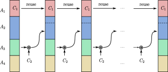
Figure 3: Chaining construction for block Markov encoding

Input :  $(S_{1}^{1:n},\ldots,S_{k}^{1:n})$, $M$ local randomness (uniform random bits) and common randomness $C=(C_{1},C_{2})$ shared with Node 2: $C_{1}$ of size $\lvert A_{1}\rvert$ and $C_{2}$ of size $\lvert A_{3}\rvert$.

Output : $\left(\widetilde{V}^{1:n}_{1},\ldots,\widetilde{V}^{1:n}_{k}\right)$

if $i=1$ then

       $\widetilde{V}_{1}[A_{1}]\longleftarrow C_{1}\qquad\widetilde{V}_{1}[A_{2}]\longleftarrow M$

       for $j\in A_{3}\cup A_{4}$ do

             Given $S_{1}^{1:n}$, succ. draw the bits $\widetilde{V}_{1}^{j}$ according to

$$P_{V^{j}\mid V^{1:j-1}S^{1:n}}\left(\widetilde{V}_{1}^{j}\mid\widetilde{V}_{1}^{1:j-1}S_{1}^{1:n}\right)$$ (3)

       end for

      

end if

for $i=2,\ldots,k$ do

       $\widetilde{V}_{i}[A_{1}]\longleftarrow C_{1}\qquad\widetilde{V}_{i}[A^{\prime}_{3}]\longleftarrow\widetilde{V}_{i-1}[A_{3}]\oplus C_{2}$

       $\widetilde{V}_{i}[A_{2}\setminus A^{\prime}_{3}]\longleftarrow M$

       for $j\in A_{3}\cup A_{4}$ do

             Given $S_{i}^{1:n}$, succ. draw the bits $\widetilde{V}_{i}^{j}$ according to

$$P_{V^{j}\mid V^{1:j-1}S^{1:n}}\left(\widetilde{V}_{i}^{j}\mid\widetilde{V}_{i}^{1:j-1}S_{i}^{1:n}\right)$$ (4)

       end for

      

end for

Algorithm 1 Encoding algorithm at Node 1

In particular, the chaining construction proceeds as follows:

• since the bits in $\operatorname{\mathcal{V}}_{V|S}$ are nearly uniform and independent of $S^{1:n}$ by Definition (2), the bits in $A_{1}\subset\operatorname{\mathcal{V}}_{V|S}$ are chosen with uniform probability using a uniform randomness source $C_{1}$ shared with Node 2, and their value is reused over all blocks;

• in the first block the bits in $A_{2}\subset\operatorname{\mathcal{V}}_{V|S}$ are chosen with uniform probability using a local randomness source $M$;

• for the following blocks, let $A^{\prime}_{3}$ be a subset of $A_{2}$ such that $\lvert A^{\prime}_{3}\rvert=\lvert A_{3}\rvert$. The bits of $A_{3}$ in block $i$ are sent to $A^{\prime}_{3}$ in the block $i+1$ using a one time pad with key $C_{2}$. Thanks to the Crypto Lemma [19, Lemma 3.1], if we choose $C_{2}$ of size $\lvert A_{3}\rvert$ to be a uniform random key, the bits in $A^{\prime}_{3}$ in the block $i+1$ are uniform. The bits in $A_{2}\setminus A^{\prime}_{3}$ are chosen with uniform probability using the local randomness source $M$;

• the bits in $A_{3}$ and in $A_{4}$ are generated according to the previous bits using successive cancellation encoding [17]. Note that it is possible to sample efficiently from $P_{V^{i}\mid V^{1:i-1}S^{1:n}}$ given $S^{1:n}$ [17].

The encoder then computes $\widetilde{U}_{i}^{1:n}=\widetilde{V}_{i}^{1:n}G_{n}$ for $i=1,\ldots,k$ and generates $X_{i}^{1:n}$ symbol by symbol from $\widetilde{U}_{i}^{1:n}$ and $S_{i}^{1:n}$ using the conditional distribution

$$P_{X_{i}^{j}|\widetilde{U}_{i}^{j}S_{i}^{j}}(x|\widetilde{u}_{i}^{j},s_{i}^{j})=P_{X|US}(x|u_{i}^{j},s_{i}^{j})$$

and sends $X_{i}^{1:n}$ over the channel.

We use an extra $(k+1)$-th block to send a version of $V_{k}[A_{3}]$ encoded with a good channel code. In particular, this can be done using the polar code construction for asymmetric channels stated in [20]. Let $Z^{1:n}=X^{1:n}G_{n}$ be the polarized version of $X^{1:n}$. We place the information $V_{k}[A_{3}]$ in the positions of $Z^{1:n}$ indexed by $\operatorname{\mathcal{V}}_{X}\cap\operatorname{\mathcal{H}}^{c}_{X\mid Y}$. We note that $\operatorname{\mathcal{V}}_{X}\cap\operatorname{\mathcal{H}}^{c}_{X\mid Y}$ has cardinality approximately equal to $nI(X;Y)$ [20]. We have $\lvert A_{3}\rvert\leq\lvert A_{2}\rvert\leq\lvert\operatorname{\mathcal{V}}_{V}\cap\operatorname{\mathcal{H}}^{c}_{V\mid Y}\rvert$, which is approximately $nI(U;Y)$. By hypothesis, we have the Markov chain $U-X-Y$ and therefore $\lvert A_{3}\rvert\leq nI(X;Y)$. We can send the bits in $A_{3}$ with vanishing error probability. The scheme in [20] requires common randomness, which will have vanishing rate when $k$ is large enough since it’s used only in the last block, and uniform messages, which can be achieved using a one-time-pad as before. Finally, $\widetilde{X}_{k+1}^{1:n}$ is the output of the channel code described above.

III-C Decoding

Input : $(Y_{1}^{1:n},\ldots,Y_{k+1}^{1:n})$, $C=(C_{1},C_{2})$ common randomness shared with Node 1

Output : $(\widehat{V}_{1}^{1:n},\ldots,\widehat{V}_{k}^{1:n})$

for $i=k,\ldots,1$ do

       $\widehat{V}_{i}[A_{1}]\longleftarrow C_{1}$

       if $i=k$ then

            $\widehat{V}_{i}[A_{3}]\longleftarrow Y_{k+1}^{1:n}$ as in [20]

       end if

      else

            $\widehat{V}_{i}[A_{3}]\longleftarrow\widehat{V}_{i+1}[A^{\prime}_{3}]$

       end if

      for $j\in A_{2}\cup A_{4}$ do

             Successively draw the bits according to

$$\widehat{V}_{i}^{j}=\begin{cases}0\quad\mbox{if }L_{n}(Y_{i}^{1:n},V_{i}^{1:j-1})\geq 1\\ 1\quad\mbox{else}\end{cases}$$

$$L_{n}(Y_{i}^{1:n},V_{i}^{1:j-1})=\frac{P_{V_{i}^{j}\mid V_{i}^{1:j-1}Y_{i}^{1:n}}\left(0\mid\widehat{V}_{i}^{1:j-1}Y_{i}^{1:n}\right)}{P_{V_{i}^{j}\mid V_{i}^{1:j-1}Y_{i}^{1:n}}\left(1\mid\widehat{V}_{i}^{1:j-1}Y_{i}^{1:n}\right)}$$

       end for

      

end for

Algorithm 2 Decoding algorithm at Node 2

The decoder observes $(Y_{1}^{1:n},\ldots,Y_{k+1}^{1:n})$ and the $(k+1)$-th block allows it to decode in reverse order. In block $i\in[1,k]$, the decoder has access to $\widehat{V}_{i}[A_{1}\cup A_{3}]=\widehat{V}_{i}[\operatorname{\mathcal{H}}_{V\mid Y}]$:

• the bits in $A_{1}$ correspond to shared randomness $C_{1}$;

• in block $k$, the bits in $A_{3}$ are recovered from $Y_{k+1}^{1:n}$ using the decoding process in [20];

• in block $i\in[1,k-1]$ the bits in $A_{3}$ are obtained by successfully recovering $A_{2}$ in block $i+1$.

For each block $i=k,\ldots,1$ the decoder recovers an estimate $\widehat{V}_{i}^{1:n}$ of $\widetilde{V}_{i}^{1:n}$ using Algorithm 2. From ${Y_{i}}^{1:n}$ and $\widehat{V}_{i}[A_{1}\cup A_{3}]$ the successive cancellation decoder can retrieve $\widehat{V}_{i}[A_{2}\cup A_{4}]$. Note that as shown in [17, Theorem 3], we have:

$$\lim_{n\rightarrow\infty}\mathbb{P}\left\{\widetilde{V}^{1:n}=\widehat{V}^{1:n}\right\}=1.$$ (5)

The decoder computes $\widehat{U}_{i}^{1:n}=\widehat{V}_{i}^{1:n}G_{n}$. Then it generates $\widehat{S}_{i}^{1:n}$ symbol by symbol using:

$$P_{\widehat{S}_{i}^{j}|\widehat{U}_{i}^{j}Y_{i}^{j}}(s|u,y)=P_{\widehat{S}|UY}(s|u,y).$$

Remark 2

The encoding and decoding complexity of this scheme is $O\left(nk\log n\right)$.

III-D Rate of common randomness

The rate of common randomness $C$ is negligible since:

$$\lim_{n\rightarrow\infty\atop k\rightarrow\infty}\frac{\lvert A_{1}\cup A_{3}\rvert}{kn}=\lim_{n\rightarrow\infty\atop k\rightarrow\infty}\frac{\lvert\operatorname{\mathcal{H}}_{V|Y}\rvert}{kn}=\lim_{k\rightarrow\infty}\frac{H(U|Y)}{k}=0.$$

IV Proof of Theorem 2

IV-A Preliminary results

We first state a few lemmas that we will need to prove Theorem 2. The proofs can be found in the Appendix.

Lemma 1

For any $i\in[1,k]$, for all $\epsilon_{0}>0$,

$$\lim_{n\rightarrow\infty}\mathbb{P}\left\{\mathbb{V}\left(T_{S^{1:n}_{i}\widetilde{U}^{1:n}_{i}},P_{SU}\right)>\epsilon_{0}\right\}=0.$$

Lemma 2

Let $P_{A}$ a distribution, $A^{1:n}$ a random vector, $B^{1:n}$ a random vector generated from $A^{1:n}$ with i.i.d. conditional distribution $P_{B|A}$ and suppose $\displaystyle\lim_{n\rightarrow\infty}\mathbb{P}\left\{\mathbb{V}\left(T_{A^{1:n}},P_{A}\right)>\epsilon\right\}=0.$ Then, for all $\epsilon^{\prime}>\epsilon$ we have:

$$\lim_{n\rightarrow\infty}\mathbb{P}\left\{\mathbb{V}\left(T_{A^{1:n}B^{1:n}},P_{AB}\right)>\epsilon^{\prime}\right\}=0.$$

Lemma 3

Let $X^{1:n}$, $\widetilde{X}^{1:n}$ two possibly dependent random sequences taking values in $\operatorname{\mathcal{X}}^{n}$ and define

$$T_{\left(X^{1:n},\widetilde{X}^{1:n}\right)}(x):=\frac{1}{2n}\sum_{i=1}^{n}\left(\mathds{1}\{X^{i}=x\}+\mathds{1}\{\widetilde{X}^{i}=x\}\right).$$

Then for any distribution $P$ on $\operatorname{\mathcal{X}}$,

$$\mathbb{V}\left(T_{\left(X^{1:n},\widetilde{X}^{1:n}\right)},P\right)\leq\frac{1}{2}\mathbb{V}\left(T_{X^{1:n}},P\right)+\frac{1}{2}\mathbb{V}\left(T_{\widetilde{X}^{1:n}},P\right).$$

Lemma 4

$\mathbb{V}\left(T_{X^{1:n}},P_{X}\right)\leq\mathbb{V}(T_{X^{1:n}Y^{1:n}},P_{XY})$.

The proof of Lemma 4 is straightforward and thus omitted.

IV-B Achievability proof

We want to show that the polar coding scheme proposed in Section III achieves empirical coordination. Given $\epsilon>0$, we want to prove that:

$$\lim_{\begin{subarray}{c}n\to\infty\\ k\to\infty\end{subarray}}\mathbb{P}\left\{\mathbb{V}\left(T_{S^{1:n}_{1:k+1}X^{1:n}_{1:k+1}Y^{1:n}_{1:k+1}\widehat{S}^{1:n}_{1:k+1}},P_{SXY\widehat{S}}\right)>\epsilon\right\}=0.$$

In order to simplify the notation, we set the joint types as

$$T :=T_{S^{1:n}_{1:k+1}\widetilde{U}^{1:n}_{1:k+1}X^{1:n}_{1:k+1}Y^{1:n}_{1:k+1}\widehat{S}^{1:n}_{1:k+1}},$$

$$T_{i} :=T_{S^{1:n}_{i}\widetilde{U}^{1:n}_{i}X^{1:n}_{i}Y^{1:n}_{i}\widehat{S}^{1:n}_{i}}\quad i\in[1,k+1].$$

Lemma 1 states that for $i\in[1,k]$ and for all $\epsilon_{0}>0$,

$$\lim_{n\rightarrow\infty}\mathbb{P}\left\{\mathbb{V}\left(T_{S^{1:n}_{i}\widetilde{U}^{1:n}_{i}},P_{SU}\right)>\epsilon_{0}\right\}=0.$$

Then, because of Lemma 2, we have that for all $\epsilon^{\prime}>\epsilon_{0}$

$$\lim_{n\rightarrow\infty}\mathbb{P}\left\{\mathbb{V}\left(T_{S^{1:n}_{i}\widetilde{U}^{1:n}_{i}X^{1:n}_{i}Y^{1:n}_{i}},P_{SUXY}\right)>\epsilon^{\prime}\right\}=0.$$

We can apply Lemma 2 again and add $\widehat{S}$, but since $\widehat{S}$ is generated by $\widehat{U}$ and not by $\widetilde{U}$, we need the conditional probability: $\forall\epsilon>\epsilon^{\prime}$ for $i\in[1,k]$ we have

$$\lim_{n\rightarrow\infty}\mathbb{P}\left\{\mathbb{V}\left(T_{i},P_{SUXY\widehat{S}}\right)>\epsilon\Big{|}\widehat{U}_{i}^{1:n}=\widetilde{U}_{i}^{1:n}\right\}=0$$

We can write:

$$\mathbb{P}\left\{\mathbb{V}\left(T_{i},P_{SUXY\widehat{S}}\right)>\epsilon\right\}$$

$$=\mathbb{P}\left\{\mathbb{V}\left(T_{i},P_{SUXY\widehat{S}}\right)>\epsilon\Big{|}\widehat{U}_{i}^{1:n}=\widetilde{U}_{i}^{1:n}\right\}\mathbb{P}\left\{\widehat{U}_{i}^{1:n}=\widetilde{U}_{i}^{1:n}\right\}$$

$$+\mathbb{P}\left\{\mathbb{V}\left(T_{i},P_{SUXY\widehat{S}}\right)>\epsilon\Big{|}\widehat{U}_{i}^{1:n}\neq\widetilde{U}_{i}^{1:n}\right\}\mathbb{P}\left\{\widehat{U}^{1:n}_{i}\neq\widetilde{U}^{1:n}_{i}\right\}.$$

Note that the last term tends to 0 since $\widetilde{U}^{1:n}$ is equal to $\widehat{U}^{1:n}$ with high probability because of (5). Hence for $i\in[1,k]$ we have

$$\lim_{n\rightarrow\infty}\mathbb{P}\left\{\mathbb{V}\left(T_{i},P_{SUXY\widehat{S}}\right)>\epsilon\right\}=0.$$

The convergence in probability of $T$ to $P_{SUXY\widehat{S}}$ follows from the convergence in probability of $T_{i}$ to $P_{SUXY\widehat{S}}$ for $i\in[1,k]$ (coordination in the first $k$ blocks). In fact, observe that by Lemma 3,

$$\mathbb{V}\left(T,P_{SUXY\widehat{S}}\right)\leq\frac{1}{k+1}\sum_{i=1}^{k+1}\mathbb{V}\left(T_{i},P_{SUXY\widehat{S}}\right).$$

This implies that:

$$\begin{split}&\mathbb{E}_{T}\left[\mathbb{V}\left(T,P_{SUXY\widehat{S}}\right)\right]\\ &\leq\frac{1}{k+1}\sum_{i=1}^{k+1}\mathbb{E}_{T}\left[\mathbb{V}\left(T_{i},P_{SUXY\widehat{S}}\right)\right].\end{split}$$ (6)

The right hand side in (6) goes to zero since:

• for $i\in[1,k]$ we already have the convergence in probability of $\mathbb{V}\left(T_{i},P_{SUXY\widehat{S}}\right)$ to zero, therefore the convergence in mean since $\mathbb{V}\left(T_{i},P_{SUXY\widehat{S}}\right)$ is bounded for all $i$;

• for $i=k+1$, since $T_{k+1}$ and $P_{SUXY\widehat{S}}$ are probability distributions, $\mathbb{V}\left(T_{k+1},P_{SUXY\widehat{S}}\right)\leq 2.$ For $k$ large enough $2/(k+1)$ goes to zero, then $\mathbb{E}[2]/(k+1)=2/(k+1)$ goes to zero and empirical coordination still holds.

Then, the left hand side in (6) goes to zero and because convergence in mean implies convergence in probability, we have the convergence in probability of $\mathbb{V}\left(T,P_{SUXY\widehat{S}}\right)$ to zero. To complete the proof we recall that because of Lemma 4, $\mathbb{V}\left(T,P_{SUXY\widehat{S}}\right)<\epsilon$ implies that

$$\mathbb{V}\left(T_{S^{1:n}_{1:k+1}X^{1:n}_{1:k+1}Y^{1:n}_{1:k+1}\widehat{S}^{1:n}_{1:k+1}},P_{SXY\widehat{S}}\right)<\epsilon.$$

-C Proof of Lemma 1

For all $\epsilon_{0}>0$, we define

$$\mathcal{T}_{\epsilon_{0}}\left(P_{SU}\right):=\left\{(S^{1:n},U^{1:n})\big{|}\mathbb{V}\left(T_{S^{1:n}U^{1:n}},P_{SU}\right)\leq\epsilon_{0}\right\}$$

$$\mathbb{P}_{P_{SU}}\left\{(s^{1:n},u^{1:n})\in\mathcal{T}_{\epsilon_{0}}\left(P_{SU}\right)\right\}:=$$

$$\quad\sum_{s^{1:n},u^{1:n}}P_{S^{1:n}U^{1:n}}\left(s^{1:n},u^{1:n}\right)\mathds{1}\left\{(s^{1:n},u^{1:n})\in\mathcal{T}_{\epsilon_{0}}\left(P_{SU}\right)\right\}.$$

Note that $\lim_{n\rightarrow\infty}\mathbb{P}_{P_{SU}}\left\{(s^{1:n},u^{1:n})\in\mathcal{T}_{\epsilon_{0}}\left(P_{SU}\right)\right\}=1$.

Let $i\in[1,k]$, we have:

$$\mathbb{P}_{P_{S\widetilde{U}}}\left\{\mathbb{V}\left(T_{S^{1:n}_{i}U^{1:n}_{i}},P_{SU}\right)>\epsilon_{0}\right\}$$

$$=\sum_{s^{1:n},u^{1:n}}P_{S^{1:n}_{i}\widetilde{U}^{1:n}_{i}}\left(s^{1:n},u^{1:n}\right)\mathds{1}\left\{(s^{1:n},u^{1:n})\notin\mathcal{T}_{\epsilon_{0}}\left(P_{SU}\right)\right\}$$

$$=\sum_{s^{1:n},u^{1:n}}(P_{S^{1:n}_{i}\widetilde{U}^{1:n}_{i}}\left(s^{1:n},u^{1:n}\right)-P_{S^{1:n}U^{1:n}}\left(s^{1:n},u^{1:n}\right)$$

$$+P_{S^{1:n}U^{1:n}}\left(s^{1:n},u^{1:n}\right))\mathds{1}{\left\{(s^{1:n},u^{1:n})\notin\mathcal{T}_{\epsilon_{0}}\left(P_{SU}\right)\right\}}$$

$$\leq\mathbb{V}(P_{S^{1:n}\widetilde{U}^{1:n}},P_{S^{1:n}U^{1:n}})+\mathbb{P}_{P_{SU}}\left\{(s^{1:n},u^{1:n})\notin\mathcal{T}_{\epsilon_{0}}\left(P_{SU}\right)\right\}$$

which tends to 0 thanks to a typicality argument and the following result.

Lemma 5

For any $i\in[1,k]$, let $\delta_{n}=2^{-n^{\beta}}$ for some $0<\beta<1/2$

$$\mathbb{V}\left(P_{U^{1:n}S^{1:n}},{P}_{\widetilde{U}_{i}^{1:n}S_{i}^{1:n}}\right)\leq\sqrt{2\log 2}\sqrt{n\delta_{n}}.$$

Proof:

We have

$$\mathbb{D}\left(P_{U^{1:n}S^{1:n}}\Big{\Arrowvert}P_{\widetilde{U}_{i}^{1:n}S_{i}^{1:n}}\right){\overset{{(a)}}{=}}\mathbb{D}\left(P_{V^{1:n}S^{1:n}}\Big{\Arrowvert}{P}_{\widetilde{V}_{i}^{1:n}S_{i}^{1:n}}\right)$$

$${\overset{{(b)}}{=}}\mathbb{D}\left(P_{V^{1:n}|S^{1:n}}\Big{\Arrowvert}{P}_{\widetilde{V}_{i}^{1:n}|S_{i}^{1:n}}\Big{|}P_{S^{1:n}}\right)$$

$${\overset{{(c)}}{=}}\sum_{j=1}^{n}\mathbb{D}\left(P_{V^{j}|V^{1:j-1}S^{1:n}}\Big{\Arrowvert}{P}_{\widetilde{V}_{i}^{j}|\widetilde{V}_{i}^{1:j-1}S_{i}^{1:n}}\Big{|}P_{V^{1:j-1}S^{1:n}}\right)$$

$${\overset{{(d)}}{=}}\sum_{j\in A_{1}\cup A_{2}}\mathbb{D}\left(P_{V^{j}|V^{1:j-1}S^{1:n}}\Big{\Arrowvert}{P}_{\widetilde{V}_{i}^{j}|\widetilde{V}_{i}^{1:j-1}S_{i}^{1:n}}\Big{|}P_{V^{1:j-1}S^{1:n}}\right)$$

$${\overset{{(e)}}{=}}\sum_{j\in A_{1}\cup A_{2}}\left(1-H(V^{j}\mid V^{1:j-1}S^{1:n})\right){\overset{{(f)}}{<}}\delta_{n}\lvert\mathcal{V}_{V\mid S}\rvert\leq n\delta_{n},$$

where $(a)$ comes from the invertibility of $G_{n}$, $(b)$ and $(c)$ come from the chain rule, $(d)$ comes from (3) and (4), $(e)$ comes from the fact that the conditional distribution $P_{\widetilde{V}_{i}^{j}|\widetilde{V}_{i}^{1:j-1}S_{i}^{1:n}}$ is uniform for $j$ in $A_{1}$ and $A_{2}$ and $(f)$ from (2). Then, the proof is completed using Pinsker’s inequality. ∎

-D Proof of Lemma 2

We have:

$$\mathbb{P}\left\{\mathbb{V}\left(T_{A^{1:n}B^{1:n}},P_{AB}\right)>\epsilon^{\prime}\right\}\leq\mathbb{P}\left\{\mathbb{V}\left(T_{A^{1:n}},P_{A}\right)>\epsilon\right\}+$$

$$\mathbb{P}\left\{\mathbb{V}\left(T_{A^{1:n}},P_{A}\right)\leq\epsilon\right\}\mathbb{P}\left\{\mathbb{V}\left(T_{A^{1:n}B^{1:n}},P_{AB}\right)>\epsilon^{\prime}\big{|}\mathbb{V}\left(T_{A^{1:n}},P_{A}\right)\leq\epsilon\right\}.$$

Then as $n$ goes to infinity, the first term tends to zero by the conditional typicality lemma [21] and the second tends to zero by hypothesis.

-E Proof of Lemma 3

The statement follows from the inequalities:

$$\big{\lvert}T_{\left(X^{n},\widetilde{X}^{n}\right)}(x)-P(x)\big{\rvert}$$

$$=\Bigg{\lvert}\frac{1}{2}\sum_{i=1}^{n}\left(\frac{\mathds{1}\{X^{i}=x\}}{n}+\frac{\mathds{1}\{\widetilde{X}^{i}=x\}}{n}\right)-\frac{P(x)}{2}-\frac{P(x)}{2}\Bigg{\rvert}$$

$$\leq\frac{1}{2}\Bigg{\lvert}\sum_{i=1}^{n}\frac{\mathds{1}\{X^{i}=x\}}{n}-P(x)\Bigg{\rvert}+\frac{1}{2}\Bigg{\lvert}\sum_{i=1}^{n}\frac{\mathds{1}\{\widetilde{X}^{i}=x\}}{n}-P(x)\Bigg{\rvert}.$$

References

- [1] P. W. Cuff, H. H. Permuter, and T. M. Cover, “Coordination capacity,” IEEE Transactions on Information Theory, vol. 56, no. 9, pp. 4181–4206, 2010.
- [2] R. Blasco-Serrano, R. Thobaben, and M. Skoglund, “Polar codes for coordination in cascade networks,” in Proc. of International Zurich Seminar on Communications, 2012, pp. 55–58.
- [3] M. R. Bloch, L. Luzzi, and J. Kliewer, “Strong coordination with polar codes,” in Proc. of Allerton Conference on Communication, Control and Computing, 2012, pp. 565–571.
- [4] R. A. Chou, M. R. Bloch, and J. Kliewer, “Polar coding for empirical and strong coordination via distribution approximation,” in Proc. of IEEE International Symposium on Information Theory (ISIT), 2015, pp. 1512–1516.
- [5] B. Larrousse, S. Lasaulce, and M. Wigger, “Coordinating partially-informed agents over state-dependent networks,” in Proc. of IEEE Information Theory Workshop (ITW), 2015, pp. 1–5.
- [6] M. Le Treust, “Correlation between channel state and information source with empirical coordination constraint,” in Proc. of IEEE Information Theory Workshop (ITW), 2014, pp. 272–276.
- [7] M. Le Treust, “Empirical coordination with two-sided state information and correlated source and state,” in Proc. of IEEE International Symposium on Information Theory (ISIT), 2015, pp. 466–470.
- [8] P. Cuff and C. Schieler, “Hybrid codes needed for coordination over the point-to-point channel,” in Proc. of Allerton Conference on Communication, Control and Computing, 2011, pp. 235–239.
- [9] M. Le Treust, “Empirical coordination for joint source-channel coding,” arXiv preprint arXiv:1406.4077, 2014.
- [10] O. Gossner, P. Hernandez, and A. Neyman, “Optimal use of communication resources,” Econometrica, pp. 1603–1636, 2006.
- [11] P. Cuff and L. Zhao, “Coordination using implicit communication,” in Proc. of IEEE Information Theory Workshop (ITW), 2011, pp. 467–471.
- [12] B. Larrousse and S. Lasaulce, “Coded power control: Performance analysis,” in Proc. of IEEE International Symposium on Information Theory (ISIT), 2013, pp. 3040–3044.
- [13] B. Larrousse, S. Lasaulce, and M. Bloch, “Coordination in distributed networks via coded actions with application to power control,” arXiv preprint arXiv:1501.03685, 2015.
- [14] R. A. Chou and M. R. Bloch, “Polar coding for the broadcast channel with confidential messages: A random binning analogy,” IEEE Transactions on Information Theory, vol. 62, no. 5, pp. 2410–2429, 2016.
- [15] S. H. Hassani and R. Urbanke, “Universal polar codes,” in Proc. of IEEE International Symposium on Information Theory (ISIT), 2014, pp. 1451–1455.
- [16] M. Mondelli, S. H. Hassani, I. Sason, and R. Urbanke, “Achieving Marton’s region for broadcast channels using polar codes,” IEEE Transactions on Information Theory, vol. 61, no. 2, pp. 783–800, 2015.
- [17] E. Arıkan, “Source polarization,” in Proc. of IEEE International Symposium on Information Theory (ISIT), 2010, pp. 899–903.
- [18] R. A. Chou, M. R. Bloch, and E. Abbe, “Polar coding for secret-key generation,” IEEE Transactions on Information Theory, vol. 61, no. 11, pp. 6213–6237, 2015.
- [19] M. Bloch and J. Barros, Physical-layer security: from information theory to security engineering. Cambridge University Press, 2011.
- [20] J. Honda and H. Yamamoto, “Polar coding without alphabet extension for asymmetric models,” IEEE Transactions on Information Theory, vol. 59, no. 12, pp. 7829–7838, 2013.
- [21] I. Csiszár and J. Körner, Information theory: coding theorems for discrete memoryless systems. Cambridge University Press, 2011.