Optimal and Scalable Methods to Approximate the Solutions of Large-Scale Bayesian Problems: Theory and Application to Atmospheric Inversions and Data Assimilation
Abstract
This paper provides a detailed theoretical analysis of methods to approximate the solutions of high-dimensional () linear Bayesian problems. An optimal low-rank projection that maximizes the information content of the Bayesian inversion is proposed and efficiently constructed using a scalable randomized SVD algorithm. Useful optimality results are established for the associated posterior error covariance matrix and posterior mean approximations, which are further investigated in a numerical experiment consisting of a large-scale atmospheric tracer transport source-inversion problem. This method proves to be a robust and efficient approach to dimension reduction, as well as a natural framework to analyze the information content of the inversion. Possible extensions of this approach to the non-linear framework in the context of operational numerical weather forecast data assimilation systems based on the incremental 4D-Var technique are also discussed, and a detailed implementation of a new Randomized Incremental Optimal Technique (RIOT) for 4D-Var algorithms leveraging our theoretical results is proposed.
1 Introduction
The Bayesian approach to inverse problems consists of updating a prior probability distribution of a quantity of interest conditioned on some physically-related observations. The conditioned probability distribution is called the posterior distribution. The Bayesian framework has been widely adopted to solve geophysical problems. For large-scale non-linear problems, such as those encountered in atmospheric modeling, sampling techniques (e.g., Markov Chain Monte-Carlo) to estimate the posterior distribution require prohibitively numerous integrations of the forward model that relates the inferred variables to the observations (Tarantola, 2005). Alternatively, when the forward model is linear and the probability distributions for the prior and the observations are Gaussian, the posterior probability distribution is Gaussian and can be fully characterized by its mean (i.e., the maximum-likelihood) and its error covariance matrix, for which analytical expressions are available. However, explicitly calculating the posterior error covariance matrix remains a challenging task in inverse problems for which the dimensions of the matrix are very large (Bousserez et al., 2015). As an example, the typical number of optimized variables in data assimilation (DA) systems for numerical weather prediction (NWP) is , which corresponds to a posterior error covariance matrix of dimension . In such cases, the posterior error covariance matrix cannot be explicitly represented in computer memory, and appropriate low-rank approximations are needed to extract useful information. Low-rank estimations of the posterior error covariance matrix are also useful to compute other quantities of interest such as the model resolution matrix and the Degree Of Freedom for Signal (DOFS), which characterize the information content of the inversion (Rodgers, 2000; Tarantola, 2005).
The variational approach to solving large-scale inverse problems employs tangent-linear and adjoint models with iterative gradient-based optimization algorithms to compute the maximum-likelihood of the posterior distribution. The potential of state-of-the-art optimization algorithms to provide posterior error covariance estimates as a by-product of the minimization have long been recognized (e.g., Thacker (1989); Rabier and Courtier (1992); Nocedal and Wright (2006); Müller and Stavrakou (2005)). For large-scale problems, such optimization algorithms are usually halted before full convergence, effectively only approximating the solution. Although the convergence properties of these approximations have been investigated in previous numerical experiments (e.g., Bousserez et al. (2015)), a theoretical analysis of their optimality with respect to the information content of the inversion has yet to be performed. Another approach to make large-scale inverse problems tractable is the use of ensembles to approximate the error covariances of the system. Such methods, which can be either stochastic (e.g., the Ensemble Kalman Filter (EnKF)) or deterministic (i.e., square-root formulations such as the Ensemble Adjusted Kalman Filter (EAKF)) have the advantage that they do not require the use of an adjoint model. However, the small number of ensembles used results in severe rank-deficiencies for the associated error covariance matrices. Sophisticated filtering localization techniques that help mitigate this sampling noise are the subject of intense research activities in ensemble-based DA (e.g., Ménétrier et al. (2015); Anderson and Lei (2013)).
Besides implicit (i.e., incomplete variational minimizations) and explicit (i.e., ensemble-based) low-rank approximations, another approach to approximate the solution of large-scale Bayesian problems consists of performing a prior dimensional reduction of the system. In the context of linear problems, such methods can allow one to explicitly form the matrices associated with the inverse problem and to analytically compute the posterior mean and posterior error covariance. In the atmospheric inversion community, several studies have focused on designing objective methods to construct reduced spaces, so as to optimize some criteria related to the information content of the problem. In Bocquet et al. (2011), a rigorous multi-scale approach to dimension reduction is proposed, wherein an optimal aggregation scheme is defined by constructing a grid of tiles for which the associated reduced Bayesian problem has maximum DOFS. However, the optimization of the grid can be computationally expensive, and the method requires explicitly calculation of the Jacobian of the system, which is not feasible for high-dimensional systems. Moreover, the optimality of the solution is guaranteed only for a specific class of reductions, namely grid aggregation methods. More recently, Turner and Jacob (2015) proposed a method to construct an optimal reduced basis set of Gaussian-mixture functions to analytically solve large-scale atmospheric source inversion problems. Their algorithm consists of an incremental construction of the basis where the posterior error variances in observation space are recomputed at each iteration (i.e., for each new dimension) until a minimum total error is reach. The cost associated with computing the posterior error variances at each iteration makes this approach poorly scalable and not suitable for problems where the optimal basis needs to be constructed in a timely manner. Similarly to Bocquet et al. (2011), their approach also lacks generality by restricting the analysis to a specific class of basis (namely, the Gaussian-mixture functions).
Recently, Spantini et al. (2015) presented a detailed theoretical analysis of optimal low-rank approximations of the posterior mean and posterior error covariance matrix for linear Bayesian problems. They show that the proposed approximations are defined in the subspace that maximizes the observational constraints, which is measured as the relative gain in information in the posterior with respect to the prior information. Interestingly, this method can reconcile theoretical optimality and computational scalability, since in practice the low-rank optimal approximations can be efficiently constructed by applying matrix-free singular value decomposition (SVD) routines to the so-called prior-preconditioned Hessian of the quadratic cost function. Furthermore, when high-performance computing is required, the use of recently developed randomized SVD methods allows to fully parallelize the algorithm and to implement and scalable approach to low-rank approximation for large-scale Bayesian problems (e.g., Bui-Thanh et al. (2012)).
In this paper, we provide a detailed theoretical analysis of the Bayesian approximation problem in the context of optimal projections. This approach has the advantage of producing approximations to the posterior mean and posterior error covariance matrix that are consistent with each other, i.e., they are both approximations to the full-dimensional posterior solutions and exact solutions to a projected low-rank Bayesian problem. Our mathematical developments generalize the theoretical framework of Bocquet et al. (2011) and allow us to construct a projection that maximizes the DOF among all low-rank projections. This maximum-DOFS projection yields posterior mean and posterior error covariance approximations similar to those proposed in Spantini et al. (2015), for which we provide additional interpretations and optimality results. Moreover, although Spantini et al. (2015) identified their optimal approximations as the solutions of a projected Bayesian problem with maximum observational information with respect to the prior, we note that they did not rigorously demonstrate this result by omitting to analyze the so-called representativeness error. This error, which quantifies the impact of the unobserved subspace in the inversion as a result of the dimension reduction, has been taken into account in our proofs. For the first time, this optimal approximation method is applied to a large-scale atmospheric-transport source inversion problem using a highly-scalable randomized SVD algorithm. Finally, we investigate new links between the maximum-DOFS approximations and preconditioned conjugate-gradient (CG) algorithms embedded in non-linear Gauss-Newton minimization methods such as incremental 4D-Var in operational DA systems for NWP. This enables us to propose an improved incremental 4D-Var algorithm leveraging both our theoretical optimality results and the efficiency of randomized SVD algorithms.
Section 2 of this paper presents the theory and formalism of the optimal low-rank projection problem and provides useful optimality results for the associated approximations of the posterior mean and posterior covariance matrices. Section 3 discusses the practical construction of the optimal approximations and describes in details a randomized SVD algorithm that allows highly-scalable implementation of the method. In Section 4, we present a numerical experiment to illustrate the theoretical results established in Section 2 and test the computational performance of the randomized SVD approach to implement the optimal low-rank approximations. Our example consists of a high-dimensional atmospheric-transport source inversion problem using a large dataset of satellite observations. Finally, in Section 5 we investigate the links between the proposed optimal approximations and variational optimization algorithms used in current operational DA systems for NWP, and we propose a new Randomized Incremental Optimal Technique (RIOT) for 4D-Var based on our findings.
2 Theory
2.1 The Bayesian Problem
2.1.1 Finding the Maximum Likelihood
Here we shall review the Bayesian inversion approach to finding the maximum likelihood of a set of random variables, given some prior probability distribution functions (pdf) on these variables and on a set of physically-related observations, adopting the notations generally used in the numerical weather prediction community. Formally, the vector of observations, , is related to the so-called control vector through a forward model operator, :
| (1) |
where , , , and and are the control space (of dimension ) and the observation space (of dimension ), respectively.
Assuming Gaussian pdfs for the prior () and the observations, with covariance error matrices and , respectively, the maximum likelihood can be obtained by minimizing the following cost function:
| (2) |
An analytical solution of (2) can be expressed as:
| (3) |
where is the Jacobian of the forward model. By applying the Shermann-Morrison-Woodbury formula to (3) (Sherman and Morrison, 1949), an alternative expression can be obtained:
| (4) |
Equations (4) and (3) differ significantly in term of practical implementation. Eq. (4) requires forming and inverting the () matrix , while in Eq. (3) the () matrix is inverted. The matrix is called the matrix of innovation statistics, and it plays an important role in DA methods.
For the common class of problems associated with a large control vector (e.g., ) but a small number of observations , provided that a tangent linear (i.e., an implicit ) and an adjoint (i.e., an implicit ) models are available, it may be possible to explicitly form and invert the matrix of innovation statistics and to compute the maximum likelihood exactly using Eq. (4) (note that in this case would need to be defined implicitly as well). This approach is at the core of the representer method (Bennett, 2005), which is similar to the so-called Physical Space Assimilation System (PSAS). Note that in practice adjoint and tangent-linear model integrations are required to extract the columns of . Although parallel implementation is possible to compute those columns, operational constraints (e.g., in NWP) and the limitation of computer resources may render this method impractical even for moderately large (e.g., ). In the case where is small enough, the maximum likelihood solution can be obtained following a similar approach, but using (3) instead of (4). The formulation is sometimes used in ensemble-based DA methods (e.g., EAKF) (Anderson, 2001), where a small number of perturbed trajectories is used to produce a sample estimate of . If neither of the analytical formulations (4) and (3) can be directly used (e.g., if both and are very large), a variational optimization approach consisting of minimizing the cost function (2) is usually the method of choice, provided an adjoint model is available. However, solutions obtained from iterative minimization techniques are often only approximations to the maximum likelihood solution, since in practice the iteration is halted before full convergence is reached.
In the present study, we shall assume that is very large () and propose optimal approximations to the Bayesian solution whose practical implementations present good scalability properties. The optimality criteria considered will rely on the information content of the inversion, whose rigorous definition is the object of the following Section.
2.1.2 The Linear Case: Information Content and Incremental Formulation
In this study we shall assume that the forward model is linear, so that . The non-linear case will be treated in Section 5, which investigates operational DA assimilation methods in NWP. Assuming linearity for the forward model allows us to rigorously define and compute useful quantities characterizing the information content of the inversion (Rodgers, 2000). With a linear forward model, , the posterior distribution is Gaussian and the maximum likelihood is equal to the posterior mean. If the linear approximation of the forward model is valid in a neighborhood of the maximum-likelihood, the local posterior pdf is approximately Gaussian, in which case the notion of posterior error covariance becomes (locally) meaningful. Moreover, for a linear forward model, the cost function defined in (2) becomes quadratic, and the inverse of its Hessian at the minimum is equal to the posterior error covariance matrix, that is:
| (5) |
where denotes the expectation of the random vector and represents the true state. Another useful formulation for can be obtained by applying the Shermann-Morrison-Woodbury formula to (5):
| (6) |
This formula expresses as a negative update of . The update term ( can be interpreted as the posterior error reduction afforded by the observations. Another useful metric related to the information content of the problem is the DOFS, which quantifies the number of parameters independently constrained by the observations. It can be defined as the trace of the model resolution matrix (or averaging kernel) , which represents the sensitivity of the posterior mean to the true state (Rodgers, 2000):
| (7) | |||||
| DOFs | (8) |
Finally, an additional useful formulation is to link the model resolution matrix to the posterior update term in (6):
| (9) |
From (7) we clearly see that can be interpreted as a relative posterior error reduction.
Both and characterize the information content of the inversion (in an absolute and relative sense, respectively) and will be central to our analysis. Since the triplet fully characterizes the posterior pdf and the information content of the linear Bayesian problem, it shall be referred to as the solution of the Bayesian problem. It is worth noting that in our large-scale framework the matrices and cannot be computed directly nor represented explicitly in computer memory. Meaningful approximations of these quantities are therefore needed to properly interpret the statistical significance and the information content of the estimated posterior mean. Other applications include posterior sampling strategies (e.g., in cycling DA methods), where optimal and efficient approximations of the square-root for are required (see Section 5.2.2).
In the case of a linear forward model, , the posterior update formula (4) suggests a simplification of the problem by considering the increment and innovation as the control and observation vector, respectively. The error statistics associated with the variables and are the same as those associated with and , respectively. Therefore, the previous equations defining the Bayesian solutions are unchanged when applying this change of variable. Note that in this incremental framework the prior is now the constant null vector (), whereas the true state is a random variable (). In the rest of this paper, unless specified otherwise, the control vector will be identified with the increment , and the observation vector replaced by the innovation vector .
2.1.3 Low-Rank Projections versus Low-Rank Approximations
When approximating the solution of a large-scale Bayesian problem, a fundamental distinction needs to be made between low-rank projections and low-rank approximations. A low-rank projections consists of restricting the Bayesian problem to a (small) subspace of the initial control space (by means of a projection operator). In this case a Bayesian problem of lower-rank is solved, and its solution can be considered to be an approximation of the initial problem in the sense that its posterior mean and posterior error covariance matrix converge to the true solutions as the reduced control space is (incrementally) increased. On the other hand, low-rank approximations of Bayesian problems belong to a more general class of methods that construct approximations of the posterior mean and posterior error covariance matrix of the initial high-dimensional problem, without the requirement of consistency between the approximated (low-rank) posterior mean and posterior error covariance (that is, they do not necessarily represent the posterior mean and corresponding posterior error covariance of a Bayesian problem). This distinction is important for interpretation as well as for applications of these methods. For instance, in a non-linear framework, a projection can be useful to define a low-rank version of a large-scale Bayesian problem to which MCMC sampling methods can be efficiently applied (e.g., Cui et al. (2014)). Other approximations of the same rank that do not correspond to a projected Bayesian problem may provide better estimates of the true solution, but would not be suitable for this application. In our study, we will first describe the formalism of low-rank projections and provide an optimal projection for the Bayesian problem that maximizes the information content (i.e., the DOFS) of the inversion (see Section 2.2). We will then explore the link between the solutions of this optimal projected problem and optimal low-rank approximations of the posterior mean and posterior error covariance matrix (Section 2.3).
2.2 Low-Rank Projections
2.2.1 General Formulation
One way to reduce the computational cost associated with solving a large-scale Bayesian problem is to project the problem onto a small subspace, , of dimension . By construction, the projection restricts the posterior updates to the prior mean () and to the prior error covariance matrix to the subspace , which effectively amounts to solving a problem of dimension . The projection can be chosen so as to optimize some criteria, usually related to the information content of the inversion (e.g., maximum DOF or minimum posterior error covariance matrix for some norm). An important aspect of the projection is that it may induce an additional observational error if the observed subspace (i.e., the orthogonal of the kernel of ) is not included in the range of the projector. This additional term is the so-called representativeness error. In the following we shall rigorously define the projected Bayesian problem and provide an analytical expression for the representativeness error.
Definition 2.1 (Projected Bayesian Problem).
Let us consider a Bayesian problem defined by (using the definitions in Section 2.1.1), and a projection operator (i.e, ). The projected problem associated with is the Bayesian problem , where , and , , and are the forward model, prior and observation error covariance matrices, respectively, in some basis of and .
The observational error covariance matrix () of the projected problem can be expressed as a function of and :
Proposition 2.2 (Representativeness Error).
The observational error covariance matrix for the projected Bayesian problem can be expressed as the sum of the observational error covariance for the original Bayesian problem, , and a representativeness error, as follows:
| (10) |
Proof.
For the sake of clarity, below we distinguish between the control vector and its associated increment , and the observation vector and the corresponding innovation . In the incremental framework, the observational error covariance matrix can be written:
Using the independence assumption between the errors in the observations and in the prior, one obtains:
∎
Our goal is to find a projection that maximizes the DOFS or minimizes the posterior error covariance matrix of the Bayesian problem , in some sense to be defined thereafter. In the following we describe a two-step approach to the optimal projection problem, wherein an appropriate decomposition is used to construct a class of projectors in which the optimal solutions must lie. This restriction to a particular class of projectors allows us to greatly simplify the problem, as we show in Section 2.2.4. In addition, the two-step method yields some interesting theoretical interpretations, and can be related to previous Bayesian dimension reduction approaches, as described in Sections 2.2.2 and 2.2.3.
2.2.2 A Two-Step Approach
The idea behind the projection approach is to solve a Bayesian problem of smaller dimension () than the original large-scale problem (i.e., one has ), allowing fast (sometimes analytical) computation of its solution. In this Section, a factorization of rank- projectors is proposed to construct a Bayesian problem of dimension from which the solutions of the projected problem in the canonical basis of can be derived with simple transformations. Let us recall that any projector is defined by its null space and its range, and can be written:
| (11) |
where is a matrix whose columns form an orthonormal basis for the orthogonal of the null space of , and is a matrix whose columns span the range of . In other words, defines the subspace (of dimension ) onto which the Bayesian problem is projected, while defines the direction of the projection. Another form for (11) can be derived as follows:
Proposition 2.3 (Factorization of a Projector).
Any linear operator is a projector of rank if and only if it can be written as the product of two rank- matrices, one of which is the left inverse of the other, i.e.:
| (12) |
where and two matrices of dimension and , respectively, with maximum rank and:
| (13) |
Proof.
Any projector of rank can be written , where (the range of ) and (the orthogonal of the null space of ) are two matrices of rank and dimension . Defining and , we obtain , with and of dimension and , respectively, and . Now let us consider a linear operator , with . One has also . Defining and , one sees that has the general form of a projector. ∎
Remarks 2.1.
In practice, and can be derived from the range and the null space of the projection (see previous proof). Note that the decomposition is not unique. Indeed, and verify (12) and (13) for all orthogonal matrices and (i.e., verifying ). This simply formalizes the fact that a projection is only defined by its null space and range, and is therefore basis-invariant.
The previous decomposition is now used to define a reduced Bayesian problem of dimension in order to be able to express the solution of the projected problem in the initial control space .
Definition 2.4 (Reduced Bayesian Problem).
Let us consider a projected Bayesian problem defined by . The reduced Bayesian problem associated with in the basis defined by the columns of is the problem , where and is a rank- factorization of the projector , as defined in Prop. 2.3.
The couple characterizes the correspondence between the reduced control space , on which the reduced problem is defined, and the initial control space . Note that the columns of form a basis for the subspace of on which the Bayesian problem is projected. Therefore, the vector represents the coordinates of in the basis defined by . Using the posterior solution of the reduced Bayesian problem , one can provide an analytical solution for the projected problem in the initial space :
Proposition 2.5 (Posterior Solution for a General Projection ).
Let us consider a projector , factored according to Prop. 2.3. We define the associated projected and reduced Bayesian problems, and , respectively. One has:
| (14) | |||||
| (15) | |||||
| (16) |
where and are the posterior mean of and , respectively, and are the posterior error covariance matrices of and , respectively, and and are the model resolution matrices of and , respectively. More precisely:
| (17) | |||||
| (18) | |||||
| (19) |
Or equivalently:
| (20) | |||||
| (21) | |||||
| (22) |
Here the solution is expressed in the canonical basis of the initial control space .
Proof.
Let us define the two vector spaces and . One can easily verify that the following application defines an isomorphism between and :
With this definition, associates any vector of expressed in the canonical basis of to its coordinates in the basis formed by the columns of , while associates any vector of expressed in the basis defined by to its coordinates in the canonical basis of . The prior error covariance matrix in the basis defined by is simply . Likewise, the forward model expressed in the basis defined by is simply , since: . Therefore, the Bayesian problems and are strictly equivalent ( is expressed in the particular basis defined by ). Noting , and the posterior mean, posterior error covariance and model resolution matrix, respectively, of the Bayesian problem , one can directly obtain Eq. (14) and (15) by applying . For Eq. (16), we note that the model resolution matrix of the reduced problem in the canonical basis must verify: . Using in the right-hand side, one obtains , which by identification gives Eq. (16). Formulas (17)-(19) and (20)-(22) are then obtained by replacing in (14)-(16) using Eq. (4), (6), (9), and Eq. (3), (5), (7), respectively. ∎
Remarks 2.2.
As long as the dimension of the observation space allows for explicit construction and inversion of () covariance matrices in , formulas (17)-(19) or (20)-(22) can be used to compute the posterior mean and extract any column of the posterior error covariance or model resolution matrices for the projected problem. On the other hand, when is large, due to the presence of the representativeness error and the necessity to form the matrix , it may not be practical to use either of the two formulations (17)-(19) or (20)-(22). Interestingly, as we will show in Section 2.2.4, one can define an optimal projection which has the remarkable property that it effectively avoids the need to know and evaluate the representativeness errors covariance matrix to compute the posterior solution.
Aggregations and Projections
In the multi-scale formalism presented by Bocquet et al. (2011), and are called the aggregation and prolongation operators, respectively, and is an imposed stability condition. In their study the operator consists of a weighted average of model grid cell parameters (e.g., atmospheric fluxes) and the objective is to solve an aggregated version of the initial Bayesian problem of smaller dimension, which corresponds to our reduced problem . Although Prop. 2.5 shows that the formulations for the aggregated problem and the projected problem are theoretically equivalent, their interpretations are quite different. In the projection framework, the analysis is centered on choosing a subspace of , , on which the Bayesian problem is solved, i.e., on the choice of , whose columns represent a basis of (e.g., Turner and Jacob (2015)). On the other hand, in the aggregation framework, the problem focuses on the choice of an average operator to define an aggregated problem, i.e., on . Likewise, in the projection framework the posterior solution is analyzed in , while in the aggregation framework the posterior solution for the aggregated control vector in is the meaningful quantity to interpret. Note that, from Eq. (16), the DOFS of the aggregated problem is the same as the DOFS of the associated projected problem expressed in the canonical basis of , since . In our analysis is a general operator, therefore we shall refer to it as a reduction operator (instead of an aggregation operator) and refer to as a prolongation operator for the sake of consistency with the formalism of Bocquet et al. (2011).
2.2.3 A Generalized Change of Variable for Linear Bayesian Problems
We now turn to the problem of optimizing the choice of the projection . The factorization of the projection described in the previous section will be used to construct our optimal solution in two steps. The first step consists, for a given reduction operator , of finding a prolongation operator that minimizes the representativeness error of the projected problem. The following Theorem provides such an optimal prolongation operator as a function of :
Theorem 2.6 (Optimal Prolongation).
For any reduction operator , there exists a prolongation operator such that the representativeness error is minimum w.r.t. the Löwner partial ordering. More specifically, one has:
| (23) |
where , , represents the space of real matrices, and the symbol denotes the Löwner partial ordering within the set of real positive definite matrices.
Moreover, one has:
| (24) |
Proof.
Let us rewrite the observational error covariance for the projected problem using the decomposition (2.3):
| (25) |
From Lemma (118), it is clear that minimizing is equivalent to minimizing the matrix . Fixing , we note that the solution (best prolongation ) to this minimization problem is also the Best Linear Unbiased Estimator (BLUE) of the following problem:
The BLUE solution to this problem, and therefore the optimal prolongation operator , is given by . The posterior error covariance matrix of the BLUE analysis is precisely , and it is minimum in the sense of the Löwner partial ordering among all linear estimator (i.e., among all prolongation operators) (e.g., Isotalo et al. (2008)), which proves (23). ∎
Remarks 2.3.
The optimal prolongation was first proposed by Bocquet et al. (2011), where it was derived from a Bayesian perspective exploiting the prior information. In our approach this result is obtained simply by minimizing the representativeness error.
Theorem 2.6 is a strong optimality result, since the optimality w.r.t. the Löwner partial ordering implies that the representativeness error is minimum in any direction of the observation space. This leads to the following important optimality result:
Corollary 2.7.
For any reduction operator , the prolongation operator minimizes the Fisher measurement information matrix w.r.t. the Löwner partial ordering, i.e.:
| (26) |
where and .
Theorem 2.6 and the optimal prolongation (24) yield different interpretations depending on the application. In the context of aggregation (see 2.2.2), once an aggregation operator (e.g., a weighted average of model grid-cells) has been chosen, the optimal prolongation (24) should be constructed and used together with the (reduced) forward model . On the other hand, in the context of a low-rank projection, once a subspace for the range of the projector has been chosen, Eq. (24) imposes an optimal direction for the projection. More precisely, if the columns of the matrix represent a basis for the range of the projector , then an optimal direction is defined by (i.e., in (11)). As an example of application of those concepts, we note that, in Turner and Jacob (2015), the computation of the Gaussian Mixture Model (GMM) basis defining the range of the projection is performed simultaneously with the computation of the direction of the projection, or equivalently, the operators and are constructed all at once. The fact that the resulting projection does not belong to the class of optimal projection defined in Prop. 2.11 is revealed by the presence of suboptimal features, such as a non-trivial minimum in the total posterior error variance for a rank (see interactive discussion of Turner and Jacob (2015)). Based on our results, one approach to improve the method proposed by Turner and Jacob (2015) would be to use the computed Gaussian Mixture Model (GMM) basis as range for the projection, but to replace their reduction operator (i.e., their weight matrix ) by one that corresponds to an optimal direction for the projection.
The following Proposition provides another useful optimality result for interpreting the optimal prolongation :
Proposition 2.8.
For any given reduction operator , the associated optimal prolongation operator defines a rank- projection that minimizes, over all rank- projections, the Frobenius distance between any square-root of the prior error covariance and its projection, i.e.:
| (27) |
where , and
Proof.
The proof is simply obtained by choosing a square-root of (i.e., and noting that:
Since is minimum for the Löwner partial ordering, one has in particular:
∎
Finally, a simple interpretation for the optimal couple is possible based on the following results:
Proposition 2.9 (Posterior Solution of the Reduced Bayesian Problem).
Let us define a Bayesian problem . Let us consider a reduction and its optimal prolongation , and the associated reduced Bayesian problem. One has:
| (28) | |||||
| (29) | |||||
| (30) |
where , and are the posterior mean, posterior error covariance and model resolution matrix (respectively) of , and , and are the posterior mean, posterior error covariance and model resolution matrix (respectively) of .
Proof.
Similar formulas can be obtained for the solution of the projected Bayesian problem in the canonical basis of :
Corollary 2.10 (Posterior Solution of the Projected Bayesian Problem ).
Let us define a Bayesian problem . Let us consider a reduction and its optimal prolongation , and the associated projector . One has:
| (31) | |||||
| (32) | |||||
| (33) |
where , and are the posterior mean, posterior error covariance and model resolution matrix (respectively) of , and , and are the posterior mean, posterior error covariance and model resolution matrix (respectively) of the projected Bayesian problem in the canonical basis of .
In other words, if the projector is of the form , the solution of the projected Bayesian problem is simply the projection of the solution of the initial Bayesian problem. From (2.9), it is clear that the couple can be interpreted as a generalized change of variable for the solutions of linear Bayesian problems, where the transformation can be non-invertible and defines a right inverse for . It is straightforward to verify that in the case where is invertible .
Remarks 2.4.
It is interesting to note that the posterior solution of the projected Bayesian problem is also the posterior solution of the Bayesian problem , as one can see by considering an optimal prolongation in formulas (17)-(19), and using and . The Bayesian problem has similar prior error covariance as the original problem , but corresponds to a forward model for which the modes are filtered by the projection . Note that and do not in general define the same Bayesian problem. The equality between the posterior solutions of those two problems only holds when an optimal prolongation is used.
2.2.4 An Optimal Projection
The results established in Section 2.2.3, and in particular Theorem 2.6, can be used to simplify the problem of defining an optimal low-rank projection for the Bayesian problem . Indeed, one can restrict our search to the class of projections associated with optimal prolongations, using (24). We first note that this class of projections can be redefined in a simpler form:
Proposition 2.11 (Canonical Form of Projections).
Let us define the class of projections of rank associated with optimal prolongations . One has:
| (34) |
Proof.
To prove that , we define , and note that and . To prove that , we define , which verifies . ∎
Remarks 2.5.
Prop. 2.11 allows a simple (statistical) interpretation for the optimal projections, that is, they correspond to a whitening transformation () followed by a orthogonal projection () onto a rank- subspace of , and a coloring transformation () that recovers the prior error covariances.
We can now state one of the main results of this paper, which provides an optimal low-rank projection for the linear Bayesian problem. The following Lemma provides a basis of eigenvectors for the model resolution matrix, which, together with the canonical form of Prop. 2.11, allows for construction of a projected Bayesian problem with maximum DOFS. Note that in this paper eigenvectors shall always be presented in descending order of their corresponding eigenvalues.
Lemma 2.12 (Diagonalization of the Model Resolution Matrix).
Let us consider the following eigenvalue decomposition:
| (35) |
where is the matrix whose columns are the eigenvectors of , and is a diagonal matrix whose elements are the eigenvalues of . The vectors form a basis of eigenvectors for the model resolution matrix .
Proof.
Using (9), one can write . Therefore, , and the vectors diagonalize . ∎
Theorem 2.13 (Maximum-DOFS Projection).
Let us define the matrix whose columns are the first eigenvectors of , and let us define the projector:
| (36) |
The projector maximizes the DOFS of the projected Bayesian problem among all projectors of maximum rank , i.e.:
| (37) |
where is the model resolution matrix associated with the problem .
Proof.
Let us consider a projection associated with an optimal prolongation, i.e., of the form , with an orthogonal matrix (see (34)). Replacing by this expression in (19) yields . Using the property of invariance of the trace under matrix permutation and the fact that , one obtains . By Lemma .2, the maximum of is obtained for , where is the matrix whose columns are the first eigenvectors of , , which proves (37). ∎
Remarks 2.6.
As suggested in 2.1.2, another criteria to optimize the projection is to minimize the total error variance (i.e., )). However, unlike the maximum-DOFS projection, this minimum-error projection does not have a simple analytical expression, which prevents its efficient computation. In Section 2.3, we present alternative optimal approximations of the posterior error covariance matrix whose Frobenius distance to the true posterior error covariance matrix is minimal and whose total error variance is closest to true total error variance.
Remarks 2.7.
The optimal projection defined in Thm. 2.13 has been proposed by Spantini et al. (2015). We note that in their study the projected problem is defined as . However, as discussed in the present study, it is necessary to include a representativeness error, i.e., to use instead of when defining the projected Bayesian problem. Spantini et al. (2015) overlooked this issue in their analysis, which is taken into account in our proofs.
Once the truncated eigendecomposition of is available, the posterior mean and posterior error covariance of the projected problem can be explicitly expressed as a function of the first eigenvectors and eigenvalues. Note that in its current form requires the inversion of a potentially high-dimensional matrix. In fact, one can circumvent this difficulty by noting that the eigendecomposition of can be efficiently obtained from the eigendecomposition of an auxiliary matrix called the prior-preconditioned Hessian. The following properties establish the formulas to compute the maximum-DOFS solution based on that improved implementation:
Proposition 2.14 (Posterior Solution of the maximum-DOFS Projection).
Let us define the prior-preconditioned Hessian and its eigenvalue decomposition . One has:
| (38) | ||||
| (39) |
where is the eigendecomposition of . Moreover, the solution of the maximum-DOFS projection can be expressed as:
| (40) | ||||
| (41) | ||||
| (42) |
where and the are the diagonal elements of .
Proof.
Let us first prove (38)-(39). The matrix can be rewritten:
| (43) | ||||
| (44) |
where is the SVD of the square-root of the prior-preconditioned matrix and the Shermann-Morrison-Woodbury formula was applied to derive . Replacing the square-root of by its SVD in (44) and using the fact that , one obtains:
To prove (40)-(42), we first use formulas (3), (6), and (9) for , and , respectively, and substitute in them to obtain the following expressions:
| (45) | ||||
| (46) | ||||
| (47) |
We then substitute those expressions in formulas (31)-(33) and replace by its optimal solution , which yields:
| (48) | ||||
| (49) | ||||
| (50) |
Noting in (48), and replacing by its SVD in (48)-(50), one obtains the desired formulas (40)-(42). ∎
Note that an alternative formula can be derived for Eq. (40), which has the advantage that it does not require computation of the singular vectors :
Proposition 2.15 (Alternative Formulation for Posterior Mean of Maximum-DOFS Projection).
Using the previous notations, let be the first eigenpairs of the prior-preconditioned Hessian . The posterior mean of the rank- maximum-DOFS projection can be expressed as:
| (51) |
Finally, from Prop. 2.14, one also obtained the following useful result:
Corollary 2.16.
The DOFS of the rank- projected Bayesian problem with maximum DOFS is the sum of the first eigenvalues of the model resolution matrix, i.e.:
| (55) |
Proof.
∎
2.2.5 Interpretation
Information Content of Subspaces
Using our previous analysis, a natural generalization of the concept of information content to subspaces of a linear Bayesian problem can be derived. Given a subspace of dimension defined by the basis and its associated matrix column , let us define the projection with range and direction , that is, . One can verify that belongs to the class of optimal projections defined in Prop. 2.11 by defining , and noting that and . With this particular choice for the direction of the projection , the information content of the subspace can be defined as the DOFS of the projected Bayesian problem , that is, the DOFS of the Bayesian problem projected onto that subspace along the direction that maximizes the DOFS (see Thm 2.6).
Most Informed Subspaces
Thm. 2.13 shows that the maximum-DOFS projection is constructed incrementally using . Therefore, the subspace defined by the basis , which corresponds to the range of , can be interpreted as the most informed subspace of dimension , while the vector defines the th most constrained direction.
Independently Constrained Modes
The vectors are the eigenvectors of the model resolution matrix . They can therefore be interpreted as the modes that are independently constrained by the observations, since one has (Eq. (42)) (where represents the Kronecker delta).
Projected Forward Model
Based on Rem. 2.4, one can establish a link between the posterior solutions of the maximum-DOFS projection and the posterior solutions of the Bayesian problem , which corresponds to the initial Bayesian problem, , with a projected forward model. Indeed, one can verify that the posterior solutions of can be expressed as:
| (56) | ||||
| (57) | ||||
| (58) |
The optimality properties of the low-rank update approximation (57) will be described and exploited in the following Section.
2.3 Link With Low-Rank Approximations
The maximum-DOFS projection constructed in Section 2.2.4 defines a rank- Bayesian inverse problem whose information content is maximal among all rank- projections of the initial Bayesian problem. Furthermore, the posterior mean and posterior error covariance matrix of the maximum-DOFS projection are also low-rank approximations to the initial full-dimensional posterior mean and posterior error covariance matrix, respectively. In this Section, we provide important optimality results associated with those low-rank approximations to the posterior solution. Additionally, useful optimality results associated with low-rank approximations to the posterior solution that do not correspond to projections are also provided, which can be alternatively used when only best approximations to the solution of the original Bayesian problem are sought and consistency between the approximated posterior mean and posterior errors is not required (see Section 2.1.3).
2.3.1 Optimal Low-Rank Approximations
Before establishing optimality results associated with low-rank approximations to the posterior solution, one needs to define an appropriate class of approximations. As discussed in Section 2.1.2 , a natural class of approximations for the posterior error covariance matrix is the one that corresponds to negative updates to the prior error covariance matrix. This particular class is central to our analysis, since the negative update can be interpreted as the information content of the inversion (see Section 2.1.2). We note that previous studies have already demonstrated the importance of this approximation class for metrics useful in the Bayesian framework (e.g., Spantini et al. (2015); Cui et al. (2014)).
Definition 2.17 (Classes of Approximations).
Let us define the following classes of matrices:
where defines the class of negative semidefinite updates to the prior error covariance matrix .
The approximations that belong to the class are referred to as low-rank approximations, while the approximations that belong to the class are low-rank update approximations. Therefore, the class is associated with full-rank approximations to the posterior mean update.
In the following Proposition, optimality results for several posterior error covariance matrix approximations are provided. All approximations are based on the classes defined in Def. 2.17 and on the truncated eigendecomposition of either (see Section 2.2.4) or , which are both related to the information content of the inversion.
Proposition 2.18 (Optimal Approximations of the Posterior Error Covariance).
Using the previous notations, let us define:
| (59) | ||||
| (60) |
where and are the th eigenvector and eigenvalue, respectively, of , and where is the posterior error covariance of the projected Bayesian problem .
One has the following optimality properties:
| (61) | ||||
| (62) | ||||
| (63) | ||||
| (64) | ||||
| (65) |
where:
-
•
represents the Frobenius norm.
-
•
is the weighted Frobenius norm defined by , where is a square-root of .
Proof.
The proof of (61) follows immediately from the Eckart-Young theorem [Eckart and Young, 1936], since one has .
The proofs for formulas (62)-(65) are obtained by writing:
| (66) | ||||
| (67) |
Multiplying on the left and on the right by the inverse of the square-root of in (66) and (67), we obtain:
Using the previous notations, a square-root of is given by . Multiplying on the left and on the right by and , respectively, in (66) and (67), we obtain:
∎
Remarks 2.8.
It has been shown in Spantini et al. (2015) that also verifies: , where is the Förstner distance, defined by , where () is the sequence of generalized eigenvalues of the pencil .
We now establish optimality results for several posterior mean approximations. In addition to the maximum-DOFS solution (), a full-rank posterior mean approximation () is considered. It is obtained by replacing the posterior error covariance implicit in Eq. (3) by the low-rank update approximation . The truncated eigendecomposition of is also exploited to define another optimal approximation of the posterior mean (). The optimality results (72) and (74) below can be found in Spantini et al. (2015). We recall the proofs here since the same principles can be applied to prove the other optimality results.
Proposition 2.19 (Optimal Approximations of the Posterior Mean).
Using the previous notations, let us define the following posterior mean approximations:
| (68) | ||||
| (69) |
where .
One has the following optimality properties:
| (70) | ||||
| (71) | ||||
| (72) | ||||
| (73) | ||||
| (74) |
where:
-
•
represent the Euclidian norm.
-
•
is the weighted Euclidian norm.
-
•
is the average operator.
-
•
is the gain matrix of the initial Bayesian problem.
Proof.
To prove (70), we use Lemma .3 and the fact that :
| (75) | ||||
| (76) |
Now, using Theorem 2.1 of Friedland and Torokhti (2007), a solution of is given by:
| (77) |
where is the truncated SVD of rank of and is a non-singular square-root of . Replacing by (79) and by in (76) yields (70).
Below we prove (72). The proof for (71) is obtained similarly. To prove (72), we also use Lemma .3 and the square-roots and of and , respectively. One has:
| (78) |
Using Theorem 2.1 of Friedland and Torokhti (2007), a solution of is therefore given by:
| (79) |
where is the rank- truncated SVD of the matrix . Further developing (79), one obtains:
Using in the expression above one obtains:
where we used the orthogonality properties of and . Finally, using
and in the right-hand side of (78) leads to , which proves (72).
Below we prove (74), (73) being obtained similarly. Using expression (3) for the posterior mean and Lemma .3, we obtain:
| (80) | ||||
| (81) |
We first note that:
Using Theorem 2.1 of Friedland and Torokhti (2007), a solution of
is given by:
where + denotes the Moore-Penrose pseudoinverse. One can verify that another minimizer of (81) is:
| (82) |
Factorizing the expression above using the square-root and its SVD like before, we obtain:
| (83) | ||||
| (84) | ||||
| (85) | ||||
| (86) |
Therefore:
| (87) |
which proves the first equality of (74). Finally, using and in (81) we obtain the equality with the right-hand side of (74). ∎
Remarks 2.9.
The approximations associated with the eigendecomposition of , i.e., and , both correspond to optimal total (non-normalized) error variance approximations. Indeed, is also the negative low-rank update to the prior error that best approximates the total error variance, i.e., .
2.3.2 Interpretation and Application
Interpretation of the Norms
The norms considered for the posterior error covariance approximations in Prop. 2.18 are all based on the Frobenius norm, which is defined as (where is the element of associated with the th row and th column), or alternatively, as (where represents the th singular value of ). Therefore, this norm accounts for all elements of the matrix in the approximation, or equivalently in the context of covariances matrices, accounts for variances in all directions (this is not the case of, e.g., the spectral norm ). Several norms in Prop. 2.18 are weighted Frobenius norms. In the case of covariance matrix approximations such as Eq. (62) to (65), those norms can be interpreted as total approximation errors normalized by the variances of the principal modes associated with the weight matrices. Indeed, one has , where is the eigendecomposition of the Hermitian matrix . The matrix can be interpreted as the covariance matrix expressed in the basis of the principal components of (i.e., the eigenvectors ), and whose variances are normalized by the variance of the principal modes (defined by the diagonal elements of ). The left and right products by and , respectively, transform the resulting matrix back into the original canonical basis. Therefore, the -weighted Frobenius norm in Prop. 2.18 measures the relative approximation error in the posterior error covariance matrix with respect to the prior errors, while the -weighted Frobenius norm measures the relative approximation error in the posterior error covariance matrix with respect to the posterior errors.
A similar analysis can be performed to interpret the statistical approximation error in the posterior mean in Prop. 2.19. Indeed, one has:
Therefore, measures the average total error in the posterior mean approximation normalized by the standard deviation of the error covariance in the principal mode directions.
Adaptive Approximations
An important consequence of Prop. 2.18 and Prop. 2.19 is that for a given rank of the approximations, an optimal strategy can be devised to minimize the normalized error in the posterior error covariance and posterior mean. Indeed, based on Eq. (62)-(65) and Eq. (71)-(74), two regimes can be distinguished: if , then and should be chosen to minimize either the -normalized or the -normalized errors in and , respectively; if is significantly greater than , then a sensible strategy would be to use the updates and to approximate and , respectively. Note that this adaptive update procedure could also be used in the context of non-linear Gauss-Newton methods to improve the convergence rate of the minimization by using an optimal update for the quadratic solution at each linearization step (see Section 5.2).
3 Practical Implementation
3.1 Remarks on Eigendecompositions
The optimal approximations of the posterior error covariance matrix and the posterior mean described in Section 2.3 rely on the eigendecompositions of the large matrices and . In the high-dimensional framework considered in our study, those matrices cannot be formed explicitly, and therefore only matrix-free SVD algorithms can be employed (i.e., algorithms that use only matrix-vector products). In addition to its many theoretical benefits, including its interpretation as the solution of a projected Bayesian problem, the maximum-DOFS approximation associated with has important computational advantages through the simplification presented in Prop. 2.14. Indeed, the SVD of does not involve direct inversions of large matrices 111Although the observation error covariance matrix can be high-dimensional and non-diagonal, in practice covariance matrices and their inverses are constructed implicitly (e.g., Singh et al. (2011)). Assuming the tangent-linear and adjoint model are available, the SVD of can be efficiently performed using matrix-free algorithms such as Lanczos or randomized SVD methods (Lanczos, 1949; Halko et al., 2011). The singular vectors computed from a truncated SVD of can be used to obtain the singular vectors used to construct the approximated posterior mean in Eq. (40), using the relation . Alternatively, a non-symmetric SVD algorithm such as that of Arnoldi (Golub and Van Loan, 2012) or Halko et al. (2011) (e.g., Alg. 5.1) can be used for direct computation of the SVD of the square-root of , . As shown in Prop. 2.15, computation of the singular vectors can be avoided using Eq. (51). However, in the context of approximated SVD, one has to keep in mind that the equality between Eq. (40) and Eq. (51) does not strictly hold. Moreover, the singular vectors can be useful for information content analysis, as discussed in Section 4.3. The possibility to efficiently compute the optimal approximations associated with the eigendecomposition of when both the control and the observation spaces are high-dimensional is in contrast with the optimal approximations associated with (i.e., and ), since algebraic simplifications similar to Prop. 2.14 do not exist for . In this case the matrix of innovation statistics needs to be formed and inverted, and a matrix-free algorithm can then be used to compute the SVD of (see Rem. 3.1).
Remarks 3.1.
In the context of atmospheric source inversion, a typical case where the number of observations is usually small enough to allow direct inversion of and compute the SVD of is the inversion of (possibly high-dimensional) sources from a sparse network of in situ observations. In contrast, satellite-based inversions, for which can be very large, may not allow to be explicitly formed, unless the dataset is reduced prior to the inversion (e.g., using an aggregation scheme).
Remarks 3.2.
In the case where the matrix of innovation statistics can be inverted explicitly, the full-dimensional analysis in Eq. (4) can be computed analytically even for control vectors with very large dimensions (as long as the tangent-linear and adjoint models are available). However, even in that case, computing optimal approximations (based on either or ) is still useful in order to quantify the information content of the inversion, since the posterior error covariance and the model resolution matrices are both of dimension . To this aim, Eq. (41), (59), (60) and (42) can be used to efficiently extract subsets of elements (e.g., the entire diagonal) from the approximated posterior error covariance or model data resolution matrices.
3.2 Randomized Singular Value Decomposition
The most widely used matrix-free SVD algorithms are based on the Lanczos method, which computes the dominant eigenvectors and eigenvalues of an Hermitian matrix using Krylov subspace iterations (Golub and Van Loan, 2012). Recently, randomized SVD methods have attracted interest due to their proven accuracy and high scalability for a large variety of problems. In this Section, we describe a randomized SVD algorithm, some of its theoretical properties, as well as a practical probabilistic error estimate for the approximation. The use of this randomized SVD method allows critical improvement in computational performance that we shall exploit in a numerical experiment in the context of large-scale atmospheric source inversions (see Section 4).
3.2.1 Principle
Randomization algorithms are powerful and modern tools to perform matrix decomposition. Some of their key advantages compared to standard Krylov subspace methods are their inherent stability and the possibility to massively parallelize the computations. Recently, Halko et al. (2011) presented an extensive analysis of the theoretical and computational properties of randomized methods to compute approximate matrix decomposition, including low-rank SVDs. The approach relies on the ability to efficiently approximate the range of a matrix using a relatively small sample of image vectors , where the input vectors are independent vectors with i.i.d. Gaussian entries. The quality of the approximation for the range of can be objectively determined by evaluating the spectral norm of the difference between the original matrix and its projection onto the subspace defined by the random images, i.e., one wants:
| (88) |
where is some tolerance level, is the spectral norm, and is the matrix whose columns form an orthonormal basis of the subspace spanned by . Once a satisfactory level of precision for the range has been reached, the SVD can be performed in the reduced space (defined by ) using dense matrix algebra, and the resulting singular vectors projected back onto the original space. Here we describe an algorithm especially adapted to the treatment of large Hermitian matrices involving expensive PDE solvers (in our case, the transport model and its adjoint ). The reader is referred to Halko et al. (2011) for a complete review and explanation of those techniques in other contexts. The following algorithm allows one to compute an approximate truncated SVD of an Hermitian matrix using the randomized approach (Halko et al., 2011). It uses only matrix-vector products, and is highly parallelizable.
Given a Hermitian matrix and a random Gaussian test matrix ():
In Algorithm 1, the products in step 1 generating the columns can be all performed in parallel, which renders this method highly scalable. In our case, the matrix-vector product amounts to integrating a PDE solver, which requires intensive computations (e.g., for the maximum DOF approximation). Therefore, assuming , the cost of the one-pass algorithm is largely dominated by step 1, the remaining steps involving dense linear algebra in small dimension.
In practice, the number of input samples is increased until relation (88) is verified. The spectral norm of the estimation error is not directly evaluated (doing so would entail computing the SVD of a large matrix, which is precisely what we want to approximate), but can be estimated a posteriori using an inexpensive probabilistic approach (see Section 3.2.2).
3.2.2 Error Analysis
The precision of the approximate SVD generated by Algorithm 1 depends on the error in the estimation of the range in (88), which itself depends (for a given number of samples) on the shape of the singular value spectra (i.e., fast or slow decay) and the dimension . The following result demonstrates this dependence by providing a bound for the average spectral error (Halko et al., 2011):
Proposition 3.1 (Average Spectral Error).
Let be a matrix with eigenvalues . Let be a orthonormal basis that approximates the range of (), generated from steps 1-2 of Algorithm 1. One has the following error bound:
| (89) |
In Prop. 3.1, is the targeted rank for the approximation, and is an oversampling parameter. Note that the smallest possible spectral error for a rank- approximation is [ref]. This formula shows that the average spectral error lies within a small polynomial factor of the theoretical minimum. In particular, one also sees that for very large the bound is not significantly modified when is increased (factor ). Moreover, increasing the oversampling parameter rapidly decreases the amplification factor . As a result, in practice using an oversampling parameter yields very good results.
In order to efficiently compute an estimate of the spectral error (88), one can use the following result, which provides a probabilistic bound based on sample error estimates available for free (Halko et al., 2011):
Proposition 3.2 ((Cost-Free) Posterior Probabilistic Error Bound For Range Approximation).
Let be a matrix. Let be an orthonormal basis that approximates the range of , generated from steps 1-2 of Algorithm 1, and a set of independent vectors with i.i.d. Gaussian entries . One has the following error bound:
| (90) | ||||
Based on this result, one sees that using only two samples () to estimate the right-hand side of (90) provides a bound on the spectral error with a probability 0.99. Note that samples of the form are computed at step 1 of Alg. 1 to construct . Therefore, a practical implementation of the a posteriori error bound estimate would be to use two samples out of the total set of samples generated at step 1 of Alg. 1 to derive the probabilistic bound in (90), while the remaining samples are used to compute . An adaptive range finder method using similar principles to build a matrix associated with a desired spectral error tolerance can also be found in (Halko et al., 2011) (see Alg. 4.2).
4 Numerical Illustrations
In this Section we first illustrate the theoretical results obtained in Section 2 using a small inverse problem (). This enables exact computation of the SVD involved in the optimal approximations of the Bayesian problem, and direct evaluation of the performance of the associated posterior mean and posterior error covariance estimates against the true solutions. We then test the performance of the algorithm for a large-scale experiment using the randomized SVD method described in Section 3.2.1.
4.1 Atmospheric Source Inversion Problem
Our numerical experiments are carried out in the context of an atmospheric transport source inversion problem. The setup consists of an Observation Simulation System Experiment (OSSE) where pseudo-observations of methane columns (XCH4) from a Short Wave Infrared (SWIR) instrument in low-earth orbit are generated and used to optimize randomly perturbed prior methane fluxes over North America. A nested domain with spatial resolution () is used and one scaling factor is optimized for each grid-cell for the month of July 2008, which corresponds to an initial control space of dimension . A uniform prior error standard deviation of 40% is assumed for the CH4 fluxes throughout the domain, with no spatial error correlations (diagonal matrix), and the observational error standard deviations are uniformly set to 8 ppb, with no spatial or temporal correlations. More information about the general configuration of this type of OSSE experiment can be found in Bousserez et al. (2016). The atmospheric transport (forward model, ) is simulated using GEOS-Chem, which is an offline atmospheric transport model widely used in the atmospheric chemistry community. The model configuration we used is described in Wecht et al. (2014). The adjoint of GEOS-Chem, also employed in our experiment, is described in Henze et al. (2007) and has been extensively used in previous sensitivity and inverse modeling studies (Kopacz et al., 2009; Jiang et al., 2011; Xu et al., 2013; Wells et al., 2015). Figure 1 shows a map of the prior CH4 emissions over North America. Emissions are geographically contrasting and highly variable. Since in our setup the prior error standard deviation is proportional to the prior emission magnitude, a similar high spatial variability is obtained for the prior error variances.
Note that the uniform diagonal matrix used in our setup implies that the matrices and as well as their associated approximations will coincide modulo a scalar multiplication (this is obviously not the case for a general matrix). This simplified configuration allows a clear interpretation of the results in term of observational constraints (e.g., all posterior error correlations are due to the observations only), while demonstrating the theoretical properties and numerical efficiency of the optimal approximations. As discussed in Section 3.1, the approximations based on the solution of the maximum-DOFS projection have clear theoretical and practical advantages compared to the approximations derived from the eigendecomposition of . Therefore, contrasting the characteristics of these two types of approximations in the general case (i.e., non-diagonal ) was not viewed as a priority for our analysis.
4.2 Convergence Analysis for a Small Problem
The convergence properties of the optimal posterior mean and posterior error covariance approximations are investigated using a reduced version of the source inversion problem described in Section 4.1. In this experiment, the control vector dimension is reduced to by selecting the model grid-cells which correspond to the first 300 highest gradients of the 4D-Var cost function (2) with respect to the emission scaling factors. With this setup, the Hessian of the cost function is explicitly calculated using the finite-difference method combined with adjoint model integrations. More specifically, the following formula is used to estimate each element of the Hessian matrix:
| (91) |
where , is the Kronecker delta, and is a small real number. For this experiment , which corresponds to a 1% perturbation of the CH4 flux for a particular grid cell. Since is symmetric, this calculation requires gradient calculations, which corresponds to forward model integrations and adjoint model integrations for the reduced problem. The fact that these gradient calculations can be performed in parallel makes the computation efficient. The inverse of the Hessian matrix provides the posterior error covariance matrix , which is used to compute the exact posterior mean using formulas (3). The prior-preconditioned Hessian is also computed explicitly from the Hessian finite-difference estimate (91) using: .
Figure 2 shows the singular value spectra of the prior-preconditioned Hessian of the reduced inverse problem. The spectra shows a fast decrease of the first 20 singular values (by an order of magnitude), followed by a slow decrease. The basis for the rank- maximum-DOFS projection is made of the first singular vectors of , which are computed exactly here. Moreover, according to Corollary 2.16, the DOFS of the inversion for a rank- optimal projection is equal to , where the are the first singular values of . The DOFS for our reduced inverse problem is 43. Figure 3 shows the -weighted error in the posterior error covariance matrix approximations and defined by Eq. (63) and (65), respectively. For the sake of simplicity only the -weighted errors are considered here. As expected, for small ranks (here, for ) the low-rank approximation is associated with a smaller error than the low-rank update approximation . However, the approximation error associated with shows an exponential decrease and is about an order of magnitude smaller than the approximation error of for .
Also shown on Fig. 3 is the relative error in the DOFS approximation for solution of the maximum-DOFS projection (), as well as the relative error in the total variance approximations and , as a function of the rank of the approximation. The results for the DOFS show that more than 80% of the information content of the inversion is captured by the first 120 modes, with a fast decrease of the error for the first third of the spectra followed by a slower decrease. Interestingly, the low-rank update posterior error covariance approximation shows much better performances than the low-rank approximation , even for small values of the rank . These results show that, for our experiment, the low-rank update approximation should be chosen when estimating posterior error variances. Overall, our numerical tests demonstrate the fast convergence of the low-rank update approximation for different information content metrics.
In addition to analyzing the convergence globally, it may be of interest to analyze the local behavior of this approximation. Figures 4 and 5 illustrate the convergence of the approximated error variances for for all control vector elements. Figure 4 represents the spatial distribution of the true posterior error variances as well as the approximated posterior error variances for the ranks , , and , while Fig. 5 shows the corresponding scatterplots and linear regression fits for each of those ranks. A very good accuracy of the approximated posterior error variances is observed for all ranks. This is further confirmed by the linear regression analysis, with a Pearson correlation coefficient of about 1 and an almost perfect regression line (1:1) for all ranks. From Fig. 5 it is evident that increasing the rank of the approximation above 40 does not significantly improve the results, which is consistent with the results obtained for the total error variance in Fig. 3.
Similarly to the posterior error covariance approximations, we now investigate the convergence properties of the posterior mean approximations described in Prop. 2.19. Again, for the sake of simplicity only the -weighted errors are considered here. Figure 6 shows the expectancy (or average) of the total -weighted error in the approximated posterior mean (or Bayes risk) for the solution of the maximum-DOFS projection and for the full-rank posterior mean approximation , as a function of the rank. The results for one single realization of the prior and the observations are also shown. The Bayes risk for each rank is calculated using Eq. (72) and (74), while the -weighted posterior mean error for one single realization is calculated by explicitly computing the error for one particular instance of the prior and observation probability distributions. As expected from the theory, for small values of the rank () the error associated with the low-rank projection is much smaller (by several order of magnitude) than the error associated with the full-rank approximation . However the full-rank approximation becomes rapidly the most accurate (for ), with an exponential decay of the error. The results for one realization of the prior and observation statistics also suggest very small deviations of the -weighted error from its mean behavior, which is consistent with previous findings in Spantini et al. (2015).
Similar to the posterior error analysis, it may be of interest to analyze locally the convergence of the approximated posterior mean, i.e., in our case, the spatial distribution of the posterior flux increments. Figure 7 shows the spatial distribution of the true and approximated posterior flux increments for the solution of the maximum-DOFS projection and the full-rank posterior increment approximation , for the ranks and . The contrast between the low-rank nature of the maximum-DOFS solution and the full-rank nature of is evident for . As shown in Fig. 6, for a rank the maximum-DOFS solution is associated with a smaller -normalized error (Bayes risk) than . Although the full-rank approximation better captures the true posterior increment distribution over large areas (e.g., Canada) compared to , those areas are associated with large posterior errors (see Figure 4), and thus are attributed less weight in the -normalized posterior mean score than regions over the east of the US domain associated with small posterior errors. The better performance of the low-rank maximum-DOFS solution over those regions with small posterior errors explains its overall better score. Consistent with our previous analysis (see Fig. 6), for , the full-rank posterior increment approximation better reproduces the spatial distribution of the true posterior increment across the whole domain, with now similar performances as the maximum-DOFS posterior increment over regions associated with small posterior errors (see, e.g., the eastern US).
4.3 Performance for a Large-Scale Experiment
In this Section we illustrate the efficiency of combining the optimal approximation methods with the randomized SVD algorithm by applying this approach to the full-dimensional source inversion problem defined in Section 4.1. Since the dimension of the control vector is now , explicitly forming the prior-preconditioned Hessian matrix and computing its SVD using dense linear algebra is not practical. Therefore, we use the One-Pass SVD algorithm described in Alg. 1 to compute the eigenvectors and eigenvalues of . The computation can be performed in parallel, since the matrix-vector products of with the columns of the random Gaussian test matrix can be performed independently. In our context, the computational cost of the method is largely dominated by the Hessian matrix-vector products used to build the basis for the reduced space (see step 1 of Alg. 1), since each of them amounts to integrating one tangent linear and adjoint model. The shape of the approximated eigenvalue spectra of , not shown here, is comparable to the one obtained with the small problem of Section 4.2, with an exponential decay followed by a long flat tail, typical of severely underconstrained inverse problems.
Figure 8 shows the probabilistic spectral error bound calculated using Prop. 3.2, as a function of the number of samples (i.e., the number of columns of ) used in the randomized SVD estimate. A fast decrease of the spectral error bound is observed for the first 100 samples, followed by a smaller decrease between 100 and 400 samples. It appears clearly that increasing the number of samples beyond 200 does not significantly reduce the spectral error bound (3), which suggests a reduced basis of 200 vectors would provide a reasonably good approximation of the range of for our problem. Here we used those 400 samples to form an orthonormal basis of the subspace in which the low-rank SVD was performed. We note that no significant differences were found in the approximated posterior error covariances or the approximated posterior mean updates between computations using 200 or 400 samples.
The analytical expressions for the posterior error covariance approximations, (Eq. (59)) and (Eq. (49)), and for the maximum-DOFS model resolution matrix approximation, (Eq. (50)), can be used to efficiently compute any matrix-vector product involving those matrices, and in particular to extract subsets of their elements. As an example, Fig. 9 shows the diagonal of the model resolution matrix of the rank- maximum-DOFs projection, which represents the observational constraints for each flux estimate. More specifically, each value on the diagonal quantifies the relative contribution of the observations to the total information content, with respect to the prior information. As discussed previously, it also corresponds to the sensitivity of the posterior mean flux to its true value (see Eq.(7)). The sum of the diagonal elements of is the DOFS for the projected problem, which is equal to 46. Therefore, 46 independent pieces of information (i.e., flux modes) can be obtained from the observational constraints. As explained in Section 2.2.4, the eigenvectors of the model resolution matrix represent precisely the modes that are independently constrained by the observations (with respect to the prior information), and are given by , where the are the first eigenvectors of the prior-preconditioned Hessian . Figure 10 shows the 1st, 2nd and 5th eigenvectors of , which in the case of a uniform diagonal matrix are therefore scalar multiples of the eigenvectors of the model resolution matrix . Additionally, the corresponding modes in observation space, that is, the left singular vectors of the square-root of , are also shown and were computed by propagating each singular vectors using the relation (see Section 3.1). As shown, the relative contribution of the observations to the information content of each posterior mode is greater than 80% for all three modes. The three modes correspond to clearly distinct geographical patterns. The results show that the satellite observations allow one to constrain CH4 emissions at high (almost grid-scale) spatial resolution over the Toronto (1st mode) and (to a lesser extent) the Los Angeles areas, but that constraints between the New York and Appalachian regions tend to be correlated. These figures illustrate the potential of the maximum-DOFS low-rank projection problem as a robust framework to objectively characterize the information content of an inversion.
In addition to providing useful tools to analyze fundamental properties of the inverse problem, the joint use of the optimal approximations with the randomized SVD approach provides a fast method to compute the posterior solution. The efficiency of the approach can be illustrated by comparing the number of iterations required for convergence of a standard iterative minimization routine with the number of samples needed for the randomized SVD to provide similar results. Figure 11 shows the posterior scaling factor increments obtained from a BFGS minimization with 40 iterations and from our adaptive posterior mean approximation method using randomized SVD computations with 200 samples. In this case, since , the approximated posterior mean chosen is (see Section 2.3.2). The results show that a parallel implementation of the randomized SVD approach using only 200 samples provides posterior flux increments comparable to 40 iterations of the BFGS algorithm over most areas (with differences rarely exceeding ). The moderate number of samples for this test allowed us to run all independent simulations in the randomized SVD algorithm simultaneously, resulting in a wall time computation of 72 mins. Comparatively, the BFGS minimization algorithm required a wall time 40 times longer than the randomized SVD, with a total of 48 hours. These results clearly illustrate the benefit of using the randomized SVD approach to drastically reduce the computational cost of large-scale inverse problems.
As discussed in Halko et al. (2011), the efficiency of randomized range approximation methods is driven by the rate of decrease of the singular value spectra, and is therefore problem-dependent. As suggested by Thm. 3.1, a sharp decrease of the singular values is associated with a more accurate estimate of the range of the matrix. We note that many inverse problems in geophysics, including atmospheric source inversion and weather data assimilation problems, generally exhibit this desirable behavior. However, for inverse problems whose singular values decay slowly, randomized power-iteration methods can still be used, which provides much more accurate results while mitigating the cost of the SVD compared to standard Krylov subspace methods. Their efficiency stems from exploiting parallel implementation of randomized estimates combined with a small number of power-iterations (Halko et al., 2011).
5 Link With Methods in Data Assimilation
In this Section we discuss some interesting links between the theory developed in this paper and methods used in operational data assimilation centers. In Section 5.1, we recall the incremental 4D-Var algorithm and its different square-root formulations, and explain how it is closely related to the maximum-DOFS low-rank projection. An overlooked issue related to the representativeness error when singular square-roots are used is also discussed. In Section 5.2, we propose an improved implementation of the incremental 4D-Var method, combining the optimality results of Section 2.3 with the randomized SVD technique described in Section 3.2.
5.1 Incremental 4D-Var
5.1.1 Principle
Most large-scale inverse problems, such as those encountered in atmospheric data assimilation, are solved by minimizing the least-squares cost function (2). Operational DA centers often use the incremental 4D-Var technique (e.g., Courtier et al. (1994)), which consists of a sequence of quadratic CG minimizations based on linearizations of the forward model. Each quadratic minimization is called an inner-loop, and is often performed using simplified tangent-linear and adjoint models. After each quadratic minimization, the updated posterior mean is propagated through the non-linear model and compared to the observations. This step, called the outer-loop, is repeated until a convergence criterion is reached.
In its original form, the linear (or quadratic) least-squares problem can be severely ill-conditioned, i.e., the gap between the eigenvalues of the Hessian of the cost function can be very large. This can prevent fast convergence of the CG algorithm. One widely used remedy is preconditioning, which consists of solving the least-squares problem in a basis where the eigenvalues of the Hessian of the cost function are as tightly clustered as possible. In the ideal case, where the Hessian is the identity matrix, the convergence is obtained in one iteration, which is why the matrix of change of basis (or preconditioner) should be constructed so as to best approximate a square-root of the Hessian. In practice, only limited prior knowledge of the Hessian is available (note that knowing this matrix perfectly amounts to solving the least-squares problem). Since the Hessian can be written as a positive low-rank update to the inverse prior error covariance matrix (), a common approach is to use the square-root of as a preconditioner, which one shall note , such as . This change of variable leads to the following least-squares problem for each inner-loop of the incremental 4D-Var algorithm:
| (92) | |||
where is the increment and the innovation.
5.1.2 Square-Root Formulations
There are two main types of square-root formulations used in current 4D-Var DA systems. The Control Variable Transform (CVT) consists of modeling the prior error covariance matrix implicitly, by projecting the control vector onto a basis where its elements are uncorrelated (i.e., their covariance matrix is the identity matrix) (Bannister, 2008). In this approach, the change of basis is constructed using operators that impose, e.g., dynamical balances, or filtering out modes of variability that one does not wish to include in the posterior update. In addition to allowing an implicit representation of a matrix that would otherwise be too large to store in computer memory ( in operational NWP), this technique provides an efficient preconditioning of the variational minimization(Courtier et al., 1994). With the CVT technique, the product of all the operators that decorrelate the control variables forms the square-root .
The other approach to the square-root formulation is the ensemble-based method. An ensemble-based square-root consists of modeling the matrix using an ensemble of forward model perturbation trajectories centered around their mean, i.e.:
| (93) |
where represents an ensemble of perturbed states and the mean of the ensemble. This approach is used, e.g., in ensemble-based DA methods such as the Ensemble Adjustment Kalman filter (EAKF) (Anderson, 2001), or the Ensemble-Variational (EnVar) algorithm (Lorenc, 2003). Localization techniques are usually required to mitigate undersampling noise in the approximated error variances and error correlations (e.g., Ménétrier et al. (2015)). In practice, it may be desirable to implement a hybrid formulation, in which B is a weighted average of a static full-rank matrix that represents, e.g., a climatology, and an ensemble-based flow-dependent matrix , so that is eventually modeled as:
| (94) |
where is made of compactly supported and space-limited covariance functions (Gaspari and Cohn, 1999), represents the Schur product between two matrices, and is a scalar verifying .
The matrix can be defined only at the initial time, , of the variational window, which is the En4DVar method, or throughout the assimilation window (4D matrix), which is the 4DEnVar (or EnVar) approach (Desroziers et al., 2014; Lorenc, 2003). Based on this very general square-root formulation of incremental 4D-Var, we will now establish some theoretical links between optimizations performed in current operational DA systems and the optimal low-rank approximation approaches presented in this study.
5.1.3 Preconditioned Conjugate-Gradient as an Optimal Low-Rank Projection
The following proposition establishes the theoretical equivalence (i.e., modulo approximation errors) between the posterior mean of the maximum-DOFS rank- projection and the solution obtained after iteration of the preconditioned CG algorithm. It stems from the close relationship between the CG algorithm and the Lanczos eigenvalue decomposition (Meurant and Strakoš, 2006).
Proposition 5.1 (Optimality of Preconditioned Conjugate-Gradient Minimizations).
Let us consider the -preconditioned least-squares minimization problem (92), where and . One notes the posterior mean of the rank- maximum-DOFS projection (40) and the solution obtained after (non-converged) iterations of a conjugate-gradient minimization starting from . One has:
| (95) |
Proof.
We first rewrite the cost function in (92):
with and .
Minimizing is therefore equivalent to solving:
Starting with , the CG algorithm at iteration produces (e.g., Golub and Van Loan (2012)):
| (96) |
where is the -dimensional Krylov subspace associated with and initialized with the vector , i.e., . One can rewrite (96):
| (97) |
where is a matrix whose columns form an orthonormal basis of . Noting that , where represents the -th eigenvector of , which is a basic property of the CG algorithm and is related to its link with the Lanczos method (Golub and Van Loan, 2012). This is equivalent to assuming . We therefore obtain the least-squares solution:
where we used and .
∎
From Proposition 5.1, we see that the solution of the preconditioned CG minimization after non-converging iterations is also the posterior mean of an optimal projection, in the sense of Prop. 2.19. Moreover, it is also the posterior mean solution of the projected Bayesian problem with maximum DOF. This latter fact is useful in term of interpretation, since it means that the non-converged solution (for the initial problem) is still the exact solution of a low-rank Bayesian problem, with an information content explicitly defined by Eq. (42). Preconditioning the CG algorithm with a square-root of the prior covariance was adopted for practical reasons in operational DA systems, that is, to improve the convergence of the minimization and to efficiently represent (implicitly) a high-dimensional matrix. Interestingly, our result provides also a theoretical justification for preconditioning the CG algorithm with a square-root of in quadratic 4D-Var minimizations. We also note that potentially better approximations of the posterior mean (i.e., , see Fig. 6) are available.
5.1.4 Singular Square-Root Formulations and Representativeness Error
In the context of Gaussian pdf assumptions and maximum likelihood estimation, the use of a non-singular matrix is required, as evident from the presence of in the cost function (2). The positive-definiteness of indicates that none of the control space directions are associated with a null probability density in the case of a Gaussian pdf. Square-root formulations of currently used in operational DA systems (CVT and/or ensemble-based) can violate this assumption. As emphasized recently by Ménétrier and Auligné (2015), in some DA systems the balance operators used to construct the CVT lead to a non-square square-root , and therefore implicitly model a singular matrix. Moreover, as previously mentioned, the number of trajectory perturbations, , used to represent in ensemble-based approaches is very small compared to the dimension of the control vector, i.e., , which also leads to singular square-roots for .
We note that preconditioned 4D-Var techniques that use a singular square-root for can be readily interpreted within the theoretical framework developed in Section 2.2. Indeed, solving the preconditioned quadratic 4D-Var minimization problem (92) with a singular square-root amounts to applying a two-step low-rank projection method, as described in Section 2.1.1, with and . In this case, it is also easy to check that the prolongation operator verifies , which makes it an optimal prolongation (see Thm. 2.6). Therefore, by Corollary 2.10, the exact solution of this singular preconditioned minimization problem (92) is the projection of the solution of the initial (full-rank) Bayesian problem, i.e., one has:
| (98) |
with . Note that (98) is verified if the matrix , which accounts for the representativeness error due to the restriction of the problem to the subspace spanned by the column of , is used in (92) instead of the initial observational error covariance matrix (i.e., (98) is the solution of the Bayesian problem . It is worthwhile to note that when singular square-roots formulations are used in operational DA systems, the initial observational error covariance () is not modified, which can theoretically lead to errors in the optimization. Since the representativeness error 2.2 cannot be computed in practice, it is useful to understand under which conditions it vanishes, which is the object of the following Proposition:
Proposition 5.2.
Let us consider a singular square-root of , and and its associated projection and representativeness error, respectively. One has:
| (99) |
where ⟂ denotes the orthogonal complement.
Proof.
The second equivalence on the right is immediate since . To show the first equivalence, let us write explicitly the representativeness error:
| (100) |
Let us decompose the (full-rank) matrix as:
| (101) |
where is an eigendecomposition of in the subspace spanned by the columns of , and is the expression of in a basis of the orthogonal complement of (i.e., ). Using (101) and the orthogonality properties, it is clear that . Therefore, one has: . Replacing this expression in (100), one obtains:
| (102) |
Using a square-root of 222 Note that , from and multiplication by and on the left and right, respectively, which guarantees the existence of a square-root for ., one can also write:
| (103) |
where . Therefore, one obtains the equivalence:
| (104) | ||||
| (105) | ||||
| (106) | ||||
| (107) | ||||
| (108) |
where we used the fact that (since is full-rank) and . ∎
Diagnosing the Representativeness Error
In practice, the right equivalence in (99) can be useful to diagnose the representativeness error. Indeed, one has the following necessary condition:
| (109) |
where we used the fact that for any two matrices and . The necessary condition on the right of (109) means that the subspace corresponding to non-zero sensitivities of the observations to the control space should be restricted to the range of the singular square-root of . We note that an approximation of both and can be obtained using the randomized range finder described in Alg. 1 (step 1 and 2) for and , respectively. If one notes an orthonormal basis for the range of and an orthonormal basis for the range of , one has: . Therefore, in the case where the orthonormal basis and are only approximations, a diagnostic for the representativeness error can consist of checking that:
| (110) |
In a cycling DA context, would need to be estimated at each DA cycle, while would be estimated only once. However, in Section 5.2 we discuss a strategy that would allow estimation of as a by-product of the minimization of (92), where the CG algorithm is replaced by a randomized SVD approach.
Remarks 5.1.
A recent study by Ménétrier and Auligné (2015) discusses the impact of singular square-root preconditionings in variational minimization. The discussion focuses on the idea that the change of variable should rigorously lead to a preconditioned background term of the cost function of the form , which can be different from the formulation always used in practice. The authors demonstrate that in the subspace where the CG minimization operates, the two background term formulations are equivalent. However, as described in the present paper (see Prop. 2.5), and since the singular preconditioning can be interpreted as an effective dimension reduction, the correct approach here is to consider () as the prior error covariance matrix of the preconditioned cost function, since it is precisely the prior error covariance of the reduced Bayesian problem (with and .). Therefore, one sees that the claim that there would be any potential inconsistency in using in the preconditioned 4D-Var minimization has no theoretical basis. The inconsistency can only arise from neglecting the representativeness error, as explained in this Section.
5.2 Improving Incremental 4D-Var
In this Section we propose some improvements to the standard 4D-Var algorithm, leveraging the results established in this paper. Description of the modifications and their justifications are provided below for each part of the algorithm.
5.2.1 Parallelization of the Inner-Loop Step and Optimal Increments
As shown in Prop. 5.1, the increment obtained after iterations of the CG algorithm in a given inner-loop approximates the rank- optimal posterior mean update associated with the linear Bayesian problem defined by the quadratic cost function (92). This stems from the fact that the CG procedure minimizes the cost function in a Krylov subspace that approximately spans the leading eigenvectors of the prior-preconditioned Hessian, . The eigendecomposition of is the basis of the two optimal posterior mean updates (40) and (68). Therefore, for each inner-loop step, either the Ritz pairs obtained from a CG minimization or the approximation of computed from a randomized SVD method can be used in combination with formula (40) or (68) to define optimal truncated posterior solutions. Assuming a large number of processors are available, our numerical experiments in Section 4 clearly suggest that replacing an iterative CG minimization algorithm by a parallel implementation of a randomized SVD computation would dramatically enhance the computational efficiency of the 4D-Var algorithm. In particular, in an operational context where only 10 inner-loop iterations can be afforded for each CG minimizations, a randomized SVD algorithm is expected to provide many more approximated eigenpairs of than the Ritz pairs. Note that in practice it may be necessary to oversample in order to obtain accurate SVD estimates (see 3.1). As discussed inHalko et al. (2011), for most problems an oversampling parameter of 10 is sufficient to obtain satisfying results, so that the number of required parallel integrations of the tangent-linear and adjoint models is roughly equal to number of eigenpairs of one wants to approximate. For the sake of simplicity, we shall use the term inner-loop to describe any quadratic minimization step of the incremental 4D-Var (i.e., any linearization step of the Gauss-Newton algorithm), even though in the context of randomized SVD methods the minimization is not performed through an iterative algorithm.
As discussed in 2.3.2, for a given inner-loop and a given approximation of eigenpairs of , an optimal approach to define the truncated solution of the quadratic minimization problem can be designed using the optimality results established in Proposition 2.19. More precisely, here we present a strategy, described in Alg. 2, that can be employed to statistically minimize the error in the approximated increments.
Based on the optimality results of Prop. 2.19, it is clear that when the choice for the increment will always yield a smaller average approximation error than . However, the choice when does not ensure a smaller average approximation error than . The rationale here is that the terms in (71) will greatly dominate the terms in (74) as soon as is significantly greater than 1. This threshold should therefore be adjusted when appropriate, depending on the typical spectra of for a given inverse problem. Indeed, as shown in our numerical experiments in Section 4.2 (Fig. 3 and Fig. 6), the approximations and can be associated with significantly lower approximation errors than and , respectively, for a number of ranks such that . In the remaining we shall use a threshold of 1 for the sake of simplicity, but in principle improved objective criteria to define this threshold based on both heuristic and theory can be derived. This is let for future work.
Remarks 5.2.
Statistically, Algorithm 2 should improve the convergence rate of incremental 4D-Var using standard CG minimizations, since by Proposition 5.1 the latter always produces the increment , which yields a greater approximation error than whenever the smallest approximated eigenvalue of verifies . Note that this method can be readily integrated into existing incremental 4D-Var systems based on CG minimizations by extracting the Ritz pairs and applying Algorithm 2 instead of using the CG solution.
Remarks 5.3.
In incremental 4D-Var, a stopping criterion needs to be defined for each inner-loop of the algorithm. In many operational DA systems, the stopping criterion corresponds to a fixed number of iterations defined by the available computing resources. Whenever possible, the choice can be improved, by, e.g., considering the absolute norm of the gradient of the cost function (92) (i.e., one wants , being the iteration number), the relative change of the cost function (i.e., ), or a more sophisticated criterion based on sufficient conditions of convergence for Gauss-Newton minimizations, such as the one described in Lawless and Nichols [2006] (i.e., ). In the context where an approximation of eigenpairs of is available and Algorithm 2 is used instead of the CG solution, the cost function and its gradient at the optimal rank- posterior mean can be evaluated around the values of the posterior means founds from Eqs. (111) and (112). When using the stopping criteria above in a randomized SVD context for instance, a minimum number of iterations translates into a minimum number of samples ( being the oversampling parameter) for the random test matrix (see Algorithm 1). Alternatively, a stopping criterion that combines the deterministic convergence criteria of Lawless and Nichols [2006] and the statistical approach of Algorithm 2 can be defined as , since this guarantees both the convergence of the Gauss-Newton algorithm and the statistical optimality of the update .
5.2.2 Optimal Posterior Perturbations in Ensemble-Based DA systems
In ensemble-based variational DA systems (e.g., EnVar), the propagation of errors from one assimilation window to the next is carried out using an ensemble of perturbed forecast trajectories that sample the posterior probability distribution. In practice, this posterior distribution needs to be evaluated at the maximum-likelihood (Tarantola, 2005). Therefore, a square-root of the posterior error covariance matrix evaluated at the last (converged) outer-loop iteration can be used to sample the posterior distribution. Two sampling strategies, one deterministic, and one stochastic, can then be adopted:
Stochastic Method
The stochastic approach to sampling, similar to an EnKF, consists of generating an ensemble of random perturbations that sample the posterior distribution, using the formula:
| (113) |
where the are independent random vectors drawn from a standard normal distribution , and is a square-root of the approximated posterior error covariance matrix.
Deterministic Method
In the deterministic approach, similar to an EAKF, the ensemble of perturbations is constructed so that it exactly verifies:
| (114) |
where and is a given approximation of .
Based on Proposition 2.18, optimal rank- posterior error covariance approximations can be constructed from the eigenpairs , of . Given an estimate of the first eigenpairs , obtained, e.g., from iterative CG minimizations or randomized SVD techniques, a adaptive strategy to approximate the square-root of the posterior error covariance matrix is provided in Algorithm 3.
Let be an approximation of the first eigenpairs of , computed at the last outer-loop iteration of an incremental 4D-Var optimization:
| (115) |
| (116) |
Both Eq. (116) and (115) can be used with a stochastic method to generate optimal posterior perturbations. The approximated square-root (116) can also be used in a deterministic approach by setting in (114). Note that the full-rank nature of (115) prevents it from being modeled as a deterministic square-root using a (necessarily) small number of perturbations .
Remarks 5.4.
The posterior square-roots (115) and (116) have also recently been proposed in Auligné et al. (2016) in the context of ensemble-variational DA for NWP. Their method (EVIL) uses the Ritz pairs obtained from the CG minimization at each inner-loop to construct the posterior square-root. The practical advantages of this approach and its better properties compared to other ensemble-based DA methods are discussed in Auligné et al. (2016). Our optimality results bring further theoretical justifications for using these posterior error square-root formulations, while providing new adaptive methods to construct the approximations for the posterior square-root and the posterior mean update. Additionally, Auligné et al. (2016) note that many Ritz pairs may be necessary to obtain an accurate posterior ensemble, which implies many iterations for the inner-loops and may not be practical for high-dimensional systems. It is further complicated by the fact that a rigorous approach would require one to use only the Ritz pairs obtained from the last inner-loop minimization, i.e., at the optimal state . This can have a significant impact when the system is highly non-linear, since in this case the Hessian matrix can be very different across inner-loops. Provided enough resources are available to perform many tangent-linear and adjoint integrations in parallel, the randomized SVD approach has the potential to approximate many more eigenpairs of the prior-preconditioned Hessian than the CG technique. In practice, it would therefore provide a more accurate approximation of the square-root of the posterior error covariance matrix at the optimal state than obtained through the framework proposed by Auligné et al. (2016).
Remarks 5.5.
Another possible way to define an approximated square-root of the posterior error covariance is to consider the preconditioner defined in Tshimanga et al. (2008), since their preconditioner effectively approximates the inverse Hessian of the 4D-Var cost function, which itself is an approximation of . In order to sample the posterior distribution, the preconditioner would be computed using only the approximated eigenpairs obtained at the last inner-loop, and the square-root constructed using the recursive formula provided in Thm. 2 of Tshimanga et al. (2008).
5.2.3 A New Randomized Incremental Optimal Technique (RIOT) for Variational Data Assimilation
Combining all the results from Section 5.2, a statistically optimal and computationally efficient ensemble-variational algorithm can be defined as follows:
Remarks 5.6.
An alternative strategy to using Alg. 1 is to use Algorithm 5.1 of Halko et al. (2011) to approximate the SVD of the square-root of the prior-preconditioned Hessian (or ). In Alg. 5.1, after application of the range finder (step 1 of Alg. 1), the operator (or ) needs to be projected onto the range , i.e., one needs to perform the product , which requires tangent linear integrations (or , which requires adjoint integrations). Since the computational cost for both algorithms is largely dominated by the tangent linear and adjoint integrations, we see that Alg. 5.1 and Alg. 5.6 present similar complexities. Interestingly, if Alg. 5.1 is applied to , one can used the random samples generated as by-product of step 1 to estimate , since one has . Therefore, Alg. 5.1 would enable a cost-free implementation of the representativeness error diagnostic (110).
Remarks 5.7.
Although Algorithm 4 has been presented in the context of a strong-constrained 4D-Var system, it is applicable to EnVar systems by formally removing the explicit time dimension, which is now implicitly included in all vectors and operators. In particular, the increments , the 4D observational operator and the prior error covariance (represented by an ensemble) are now defined throughout the assimilation window (i.e., between and ). As a result, the tangent-linear and adjoint models include only spatial interpolation and measurement sensitivity operators (e.g., satellite averaging kernels), which are much easier to develop and faster to integrate than the tangent-linear and adjoint of the NWP model. In the context of EnVar the posterior error covariances are also defined by the updated (posterior) ensemble throughout the assimilation window, so that steps 7-11 of Alg. 4 are no longer needed. Instead, steps 2-5 can be applied to each prior perturbation member to generate the posterior ensemble. The sampling noise in the posterior ensemble can then be mitigated by using an objective 4D-Var localization method, such as the one proposed in Bocquet (2016).
6 Conclusion
This paper has presented a robust theoretical and numerical study of methods to approximate the solution of large-scale Bayesian problems. Our analysis focused principally on the construction of optimal low-rank projections for potentially high-dimensional Bayesian problems, taking into account the computational constraints of this framework, and in particular the need for matrix-free algorithms. A low-rank projection that maximizes the information content (i.e., the DOFS) of the inversion, the maximum-DOFS solution, was proposed and its optimality properties with respect to the posterior error covariance matrix and posterior mean approximations were analyzed in details. These results are also compared to other useful optimal low-rank approximations that are not associated with projections of the initial Bayesian problem. An interesting aspect of the low-rank approximations derived from the maximum-DOFS solution is that they allow one to adaptively optimize the posterior mean and the posterior error covariances based on the properties of the spectra of the so-called prior-preconditioned Hessian matrix.
The performance of the optimal projection and alternate low-rank approximations are tested in the context of an atmospheric source inversion problem whose dimension is small enough to allow exact computation of the posterior solution. Our results indicate good convergence properties for both the posterior error covariances and posterior mean approximations and are consistent with the theory. A large-scale version of this experiment is also presented, where the maximum-DOFS solutions are computed using an efficient randomized SVD algorithm, whose parallel implementation dramatically improves the scalability of the SVD computation upon standard iterative matrix-free methods (e.g., the BFGS or Lanczos algorithms).
Finally, we discussed the link between the maximum-DOFS low-rank approximation and the square-root formulation of incremental 4D-Var methods used in current operational DA systems. In particular, we showed the theoretical equivalence between iterations of the preconditioned conjugate-gradient algorithm in inner-loop (quadratic) minimizations and the rank- maximum-DOFS solutions of the associated projected Bayesian problem. Leveraging both our optimality results (e.g., the use of adaptive approximations in quadratic inner-loop minimizations) and the computational efficiency of the randomized SVD algorithms, we then proposed an improved implementation of incremental 4D-Var (RIOT). This approach is very generic and can be used with any square-root formulation of incremental 4D-Var, including hybrid ensemble-4D-Var (Clayton et al., 2013).
Randomized SVD methods can be exploited to massively parallelize adjoint-based 4D-Var minimization algorithms, and as such represent an alternative approach that could rival the computational efficiency of ensemble-based DA, while preserving the full-rank nature of the variational formulation. However, adjoint-free ensemble-based approach such as EnKF or EnVar (Buehner et al., 2010) still present the advantage that they do not require the development and maintenance of an adjoint model. Currently, randomization methods fundamentally rely on the availability of an adjoint model. One challenge ahead is to design matrix-free randomization methods that could perform SVD based on the forward model only. Additionally, preconditioning techniques such as the ones proposed in Tshimanga et al. (2008) could be applied to the randomized SVD method to improve the accuracy of the inner-loop minimizations. Therefore, future studies should focus on leveraging both parallelization and preconditioning methods to maximize the efficiency of randomized SVD techniques in incremental 4D-Var.
Acknowledgments
This work was supported by the NASA GEO-CAPE Science Team grant NNX14AH02G and the NOAA grant NA14OAR4310136. This work utilized the Janus supercomputer, which is supported by the National Science Foundation (award number CNS-0821794), the University of Colorado Boulder, the University of Colorado Denver, and the National Center for Atmospheric Research. The Janus supercomputer is operated by the University of Colorado Boulder.
Appendix: Useful Lemmas and Their Proofs
Lemma .1.
If , and are two Hermitian non-negative definite matrices, and is a matrix, one has the following properties:
| (117) | ||||
| (118) |
where (respectively ) denotes the Löwner partial ordering (respectively strict) within the set of Hermitian non-negative definite matrices.
Proof.
A proof of (117) is given in Horn and Johnson (2012) (Corollary 7.7.4). We recall it here for the reader’s convenience.
Let be the spectral radius of a matrix. One has if and only if . Since for all , Hermitian matrices , one has . (117) follows immediately.
By linearity, demonstrating (118) is equivalent to demonstrating . It is easily proven by considering and . Since , in particular , which shows that .
∎
The demonstration of Theorem (2.13) requires the following lemma (see Horn and Johnson (2012), Corollary 4.3.39):
Lemma .2.
Let be a Hermitian matrix, suppose that , and let be a matrix whose columns form an orthonormal basis . Let be the eigenvalues of . Then one has:
| (119) | |||
Moreover, for each , one has:
| (120) | |||||
where (resp., ) represents the matrix whose columns are the singular vectors associated with the smallest (resp., highest) singular values of .
Proof.
This is a corollary of the so-called Poincaré separation theorem, which states that:
| (121) |
where denotes the th singular value of the matrix , the singular values being arranged in increasing order. To prove (119), one just needs to remark that the sum of the eigenvalues and the sum of the main diagonal elements of an Hermitian matrix are equal. (120) is trivial. ∎
Lemma .3.
Let us define a matrix , a random vector with covariance matrix , and a Hermitian positive-definite matrix . Let us also define the square-roots and of and , respectively, i.e., and . One has:
| (122) |
Proof.
∎
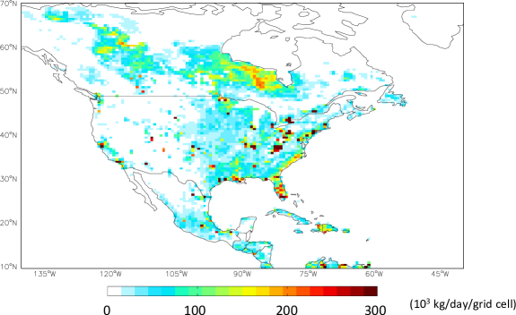

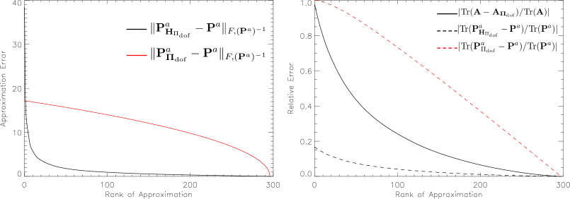
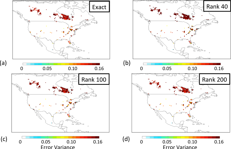
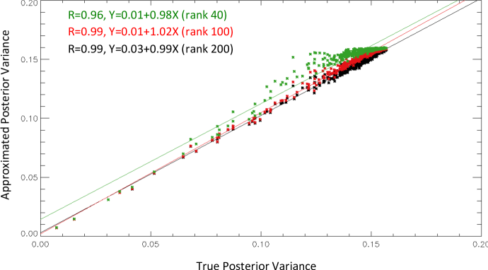
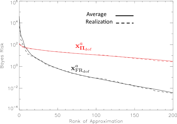
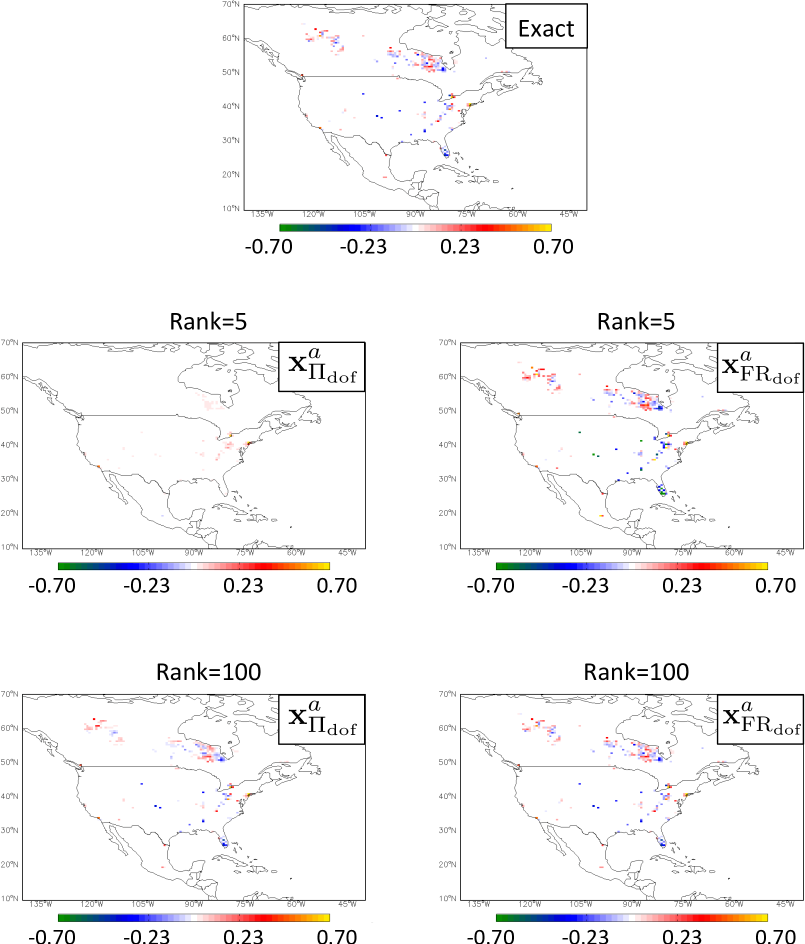

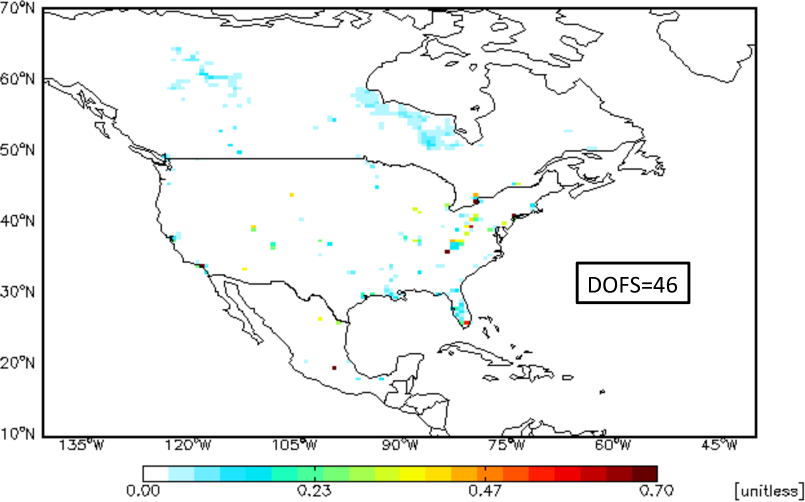
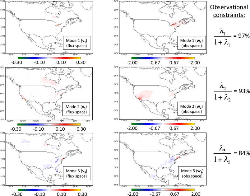
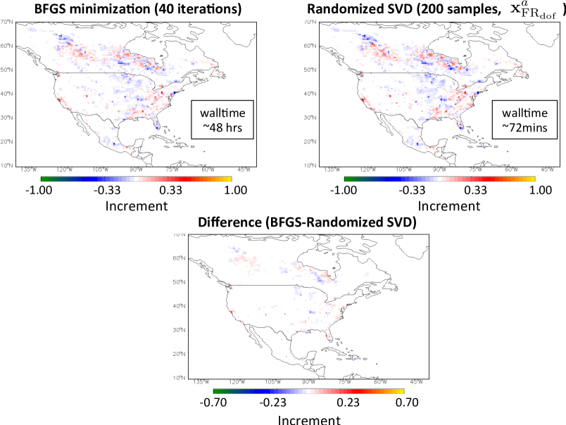
References
- Anderson (2001) Anderson J. 2001. An ensemble adjustment Kalman filter for data assimilation. Monthly Weather Review 129(12): 2884–2903.
- Anderson and Lei (2013) Anderson J, Lei L. 2013. Empirical localization of observation impact in ensemble Kalman filters. Monthly Weather Review 141(11): 4140–4153.
- Auligné et al. (2016) Auligné T, Ménétrier B, Lorenc AC, Buehner M. 2016. Ensemble-variational integrated localized data assimilation. Monthly Weather Review 144(10): 3677–3696.
- Bannister (2008) Bannister RN. 2008. A review of forecast error covariance statistics in atmospheric variational data assimilation. I : Characteristics and measurements of forecast error covariances. Quarterly Journal of the Royal Meteorological Society 134(637): 1951–1970.
- Bennett (2005) Bennett AF. 2005. Inverse modeling of the ocean and atmosphere. Cambridge University Press.
- Bocquet (2016) Bocquet M. 2016. Localization and the iterative ensemble Kalman smoother. Quarterly Journal of the Royal Meteorological Society 142(695): 1075–1089.
- Bocquet et al. (2011) Bocquet M, Wu L, Chevallier F. 2011. Bayesian design of control space for optimal assimilation of observations. Part I: Consistent multiscale formalism. Quarterly Journal of the Royal Meteorological Society 137(658): 1340–1356.
- Bousserez et al. (2015) Bousserez N, Henze D, Perkins A, Bowman K, Lee M, Liu J, Deng F, Jones D. 2015. Improved analysis-error covariance matrix for high-dimensional variational inversions: application to source estimation using a 3D atmospheric transport model. Quarterly Journal of the Royal Meteorological Society 141(690): 1906–1921.
- Bousserez et al. (2016) Bousserez N, Henze DK, Rooney B, Perkins A, Wecht KJ, Turner AJ, Natraj V, Worden JR. 2016. Constraints on methane emissions in north america from future geostationary remote-sensing measurements. Atmospheric Chemistry and Physics 16(10): 6175–6190.
- Buehner et al. (2010) Buehner M, Houtekamer P, Charette C, Mitchell HL, He B. 2010. Intercomparison of variational data assimilation and the ensemble Kalman filter for global deterministic NWP. Part I: Description and single-observation experiments. Monthly Weather Review 138(5): 1550–1566.
- Bui-Thanh et al. (2012) Bui-Thanh T, Burstedde C, Ghattas O, Martin J, Stadler G, Wilcox LC. 2012. Extreme-scale UQ for Bayesian inverse problems governed by PDEs. In: Proceedings of the International Conference on High Performance Computing, Networking, Storage and Analysis. IEEE Computer Society Press, p. 3.
- Clayton et al. (2013) Clayton A, Lorenc AC, Barker DM. 2013. Operational implementation of a hybrid ensemble/4D-var global data assimilation system at the Met Office. Quarterly Journal of the Royal Meteorological Society 139(675): 1445–1461.
- Courtier et al. (1994) Courtier P, Thepaut J, Hollingsworth A. 1994. A strategy for operational implementation of 4D-var, using an incremental approach. Quarterly Journal of the Royal Meteorological Society 120(519): 1367–1387.
- Cui et al. (2014) Cui T, Martin J, Marzouk YM, Solonen A, Spantini A. 2014. Likelihood-informed dimension reduction for nonlinear inverse problems. Inverse Problems 30(11): 114 015.
- Desroziers et al. (2014) Desroziers G, Camino JT, Berre L. 2014. 4DEnVar: link with 4D state formulation of variational assimilation and different possible implementations. Quarterly Journal of the Royal Meteorological Society 140(684): 2097–2110.
- Friedland and Torokhti (2007) Friedland S, Torokhti A. 2007. Generalized rank-constrained matrix approximations. SIAM Journal on Matrix Analysis and Applications 29(2): 656–659.
- Gaspari and Cohn (1999) Gaspari G, Cohn SE. 1999. Construction of correlation functions in two and three dimensions. Quarterly Journal of the Royal Meteorological Society 125(554): 723–757.
- Golub and Van Loan (2012) Golub GH, Van Loan CF. 2012. Matrix computations, vol. 3. JHU Press.
- Halko et al. (2011) Halko N, Martinsson PG, Tropp JA. 2011. Finding structure with randomness: Probabilistic algorithms for constructing approximate matrix decompositions. SIAM review 53(2): 217–288.
- Henze et al. (2007) Henze DK, Hakami A, Seinfeld JH. 2007. Development of the adjoint of GEOS-Chem. Atmospheric Chemistry and Physics 7(9): 2413–2433.
- Horn and Johnson (2012) Horn RA, Johnson CR. 2012. Matrix analysis. Cambridge university press.
- Isotalo et al. (2008) Isotalo J, Puntanen S, Styan GP. 2008. The BLUE’s covariance matrix revisited: A review. Journal of Statistical Planning and Inference 138(9): 2722–2737.
- Jiang et al. (2011) Jiang Z, Jones D, Kopacz M, Liu J, Henze DK, Heald C. 2011. Quantifying the impact of model errors on top-down estimates of carbon monoxide emissions using satellite observations. Journal of Geophysical Research: Atmospheres 116(D15).
- Kopacz et al. (2009) Kopacz M, Jacob DJ, Henze DK, Heald CL, Streets DG, Zhang Q. 2009. Comparison of adjoint and analytical Bayesian inversion methods for constraining asian sources of carbon monoxide using satellite (MOPITT) measurements of CO columns. Journal of Geophysical Research: Atmospheres 114(D4).
- Lanczos (1949) Lanczos C. 1949. An iteration method for solving the eigenvalue problem of linear differential operators. Bulletin of the American Mathematical Society 55(7): 717–718.
- Lorenc (2003) Lorenc AC. 2003. The potential of the ensemble Kalman filter for NWP: A comparison with 4D-Var. Quarterly Journal of the Royal Meteorological Society 129(595): 3183–3203.
- Ménétrier and Auligné (2015) Ménétrier B, Auligné T. 2015. An overlooked issue of variational data assimilation. Monthly Weather Review 143(10): 3925–3930.
- Ménétrier et al. (2015) Ménétrier B, Montmerle T, Michel Y, Berre L. 2015. Linear filtering of sample covariances for ensemble-based data assimilation. Part I: Optimality criteria and application to variance filtering and covariance localization. Monthly Weather Review 143(5): 1622–1643.
- Meurant and Strakoš (2006) Meurant G, Strakoš Z. 2006. The lanczos and conjugate gradient algorithms in finite precision arithmetic. Acta Numerica 15: 471–542.
- Müller and Stavrakou (2005) Müller J, Stavrakou T. 2005. Inversion of CO and NOx emissions using the adjoint of the IMAGES model. Atmospheric Chemistry and Physics 5: 1157–1186.
- Nocedal and Wright (2006) Nocedal J, Wright S. 2006. Numerical optimization, second edition. Numerical Optimization, Second Edition : 1–664.
- Rabier and Courtier (1992) Rabier F, Courtier P. 1992. 4-dimensional assimilation in the presence of baroclinic instability. Quarterly Journal of the Royal Meteorological Society 118(506): 649–672.
- Rodgers (2000) Rodgers CD. 2000. Inverse methods for atmospheric sounding: theory and practice, vol. 2. World scientific.
- Sherman and Morrison (1949) Sherman J, Morrison WJ. 1949. Adjustment of an inverse matrix corresponding to a change in one element of a given matrix. Annals of Mathematical Statistics 20: 317.
- Singh et al. (2011) Singh K, Jardak M, Sandu A, Bowman K, Lee M, Jones D. 2011. Construction of non-diagonal background error covariance matrices for global chemical data assimilation. Geoscientific Model Development 4(2): 299–316.
- Spantini et al. (2015) Spantini A, Solonen A, Cui T, Martin J, Tenorio L, Marzouk Y. 2015. Optimal low-rank approximations of Bayesian linear inverse problems. SIAM Journal on Scientific Computing 37(6): 2451–2487.
- Tarantola (2005) Tarantola A. 2005. Inverse problem theory and methods for model parameter estimation. SIAM.
- Thacker (1989) Thacker WC. 1989. The role of the Hessian matrix in fitting models to measurements. Journal of Geophysical Research: Oceans 94(C5): 6177–6196.
- Tshimanga et al. (2008) Tshimanga J, Gratton S, Weaver AT, Sartenaer A. 2008. Limited-memory preconditioners, with application to incremental four-dimensional variational data assimilation. Quarterly Journal of the Royal Meteorological Society 134(632): 751–769.
- Turner and Jacob (2015) Turner A, Jacob D. 2015. Balancing aggregation and smoothing errors in inverse models. Atmospheric Chemistry and Physics 15(12): 7039–7048.
- Wecht et al. (2014) Wecht KJ, Jacob DJ, Sulprizio MP, Santoni G, Wofsy SC, Parker R, Bösch H, Worden J. 2014. Spatially resolving methane emissions in California: constraints from the CalNex aircraft campaign and from present (GOSAT, TES) and future (TROPOMI, geostationary) satellite observations. Atmospheric Chemistry and Physics 14(15): 8173–8184.
- Wells et al. (2015) Wells K, Millet D, Bousserez N, Henze D, Chaliyakunnel S, Griffis T, Luan Y, Dlugokencky E, Prinn R, O’Doherty S, et al. 2015. Simulation of atmospheric N2O with GEOS-Chem and its adjoint: evaluation of observational constraints. Geoscientific Model Development 8(10): 3179–3198.
- Xu et al. (2013) Xu X, Wang J, Henze DK, Qu W, Kopacz M. 2013. Constraints on aerosol sources using GEOS-Chem adjoint and MODIS radiances, and evaluation with multisensor (OMI, MISR) data. Journal of Geophysical Research: Atmospheres 118(12): 6396–6413.