Non-trivial Interplay of Strong Disorder and Interactions
in Quantum Spin Hall Insulators Doped with Dilute Magnetic Impurities

Abstract

We investigate nonperturbatively the effect of a magnetic dopant impurity on the edge transport of a quantum spin Hall (QSH) insulator. We show that for a strongly coupled magnetic dopant located near the edge of a system, a pair of transmission anti-resonances appear. When the chemical potential is on resonance, interaction effects broaden the anti-resonance width with decreasing temperature, thus suppressing transport for both repulsive and moderately attractive interactions. Consequences for the recently observed QSH insulating phase of the $1$-T^′ of WTe₂ are briefly discussed.

I Introduction

Two-dimensional (2D) topological materials like quantum spin Hall insulators (QSHIs) have become a fascinating research topic, with many potential applications Hasan2010rmp ; exp ; review_qshi . Theoretically, QSHIs are predicted to possess gapless one-dimensional (1D) edge states XuMoore2006 ; review_qshi . Disorder potentials that are invariant under time-reversal symmetry (TRS) cannot cause Anderson localization, which is otherwise ubiquitous in 1D systems. Indeed, it has been shown WuBernevigZhang2006 ; XuMoore2006 ; Johannesson ; review_qshi that for scalar and spin-orbit (SO) disorder potentials, even in the presence of weak electron-electron interactions, the 1D edge channels of QSHIs exhibit perfect transmission, whose hallmark is a quantized conductance at low temperatures Kane20051prl . On the other hand, strong interactions can break TRS WuBernevigZhang2006 ; XuMoore2006 and lead to complex edge reconstructions Gefen ; Capone , which jeopardize the perfect conductance quantization.

Experimentally, the QSH effect arising from gapless edge channels has been observed in HgTe/CdTe and InAs/GaSb/AlSb semiconductor quantum wells (QWs) exp , graphene submitted to a strong, tilted magnetic field young , Bi $(111)$ bilayers drozdov ; yang and, more recently, in the $1$-T^′ phase of the transition metal dichalcogenide WTe₂ FuLi ; Fei2017np ; Tang ; Pablo . However, in HgTe/CdTe and InAs/GaSb/AlSb samples, long edge channels ($\sim 1\,\mu$m) in the topological phase exhibit relatively short mean-free paths, and the conductance deviates from quantization exp ; controversy ; Du1 ; Du2 . For the monolayer WTe₂, the conductance of the devices with longer edges does not exhibit the expected quantized value  Fei2017np ; Pablo . Moreover, the interpretation of the observations in InAs/GaSb QWs Du1 ; Du2 has also been questioned after the discovery of rather similar edge conduction features in the trivial phase controversy ,

Deviations from perfect conductance quantization at low temperatures arise from backscattering (BS) in the edge channels. Several BS mechanisms have been discussed using effective 1D models Schmidt ; Budich ; Lezmy ; Goldstein ; Kainaris ; review_qshi . The latter often involve electron-electron scattering in combination with scalar, spin-orbit coupling and magnetic disorder Johannesson ; Crepin ; TanakaFurusakiMateev2011 ; Budich ; Lezmy ; Goldstein ; Kainaris ; Brataas ; Liu2009prl ; Kharitonov2017 . Indeed, magnetic impurities break TRS above the Kondo temperature, and therefore they cause BS WuBernevigZhang2006 ; Maciejko ; Liu2009prl ; TanakaFurusakiMateev2011 ; Johannesson12 . Nevertheless, the connection between the effective 1D models of disorder and the 2D aspects of the physics of QSHIs has not yet been fully investigated to the best of our knowledge. With the exception of a few numerical studies in the non-interacting limit Morr ; Morr2 , there appears to be no systematic investigation about the validity of these 1D models. Indeed, little is known about whether they actually apply in the strong coupling limit where coupling strength to the impurity becomes comparable or larger than the band gap of the QSHI. The latter is an experimentally relevant regime given the small band gaps exhibited by many of the experimentally realized QSHIs. Below, we shall show that the problem of a magnetic dopant impurity problem can be mapped, in the strong coupling limit, to a generalized 1D Fano model Fano describing two resonant levels coupled to an interacting 1D channel. Using a renormalization group analysis, we show that the transmission coefficient is suppressed at low temperatures for repulsive interactions. Interestingly, when the chemical potential of the edge electrons resonates with one of the in-gap states, we find that the transmission is also suppressed for weak to moderately attractive interactions.

The rest of this article is organized as follows: Section III describes the solution of the scattering problem for a toy model of a single magnetic impurity in the neighborhood of a non-interacting QSH edge channel. In section IV, we construct an effective 1D model to describe this system, which allows us to treat the effect of weak to moderate interactions. In this section, we also discuss the effects not included in our toy model, such as the Rashba coupling in the band-structure and the non-planar alignment of the magnetic moment. Finally, in section V we offer the conclusions of this work and provide an outlook for future research directions. The Appendix contains the most technical details of the calculations. Henceforth, we work in units where $\hbar=1$.

II Model

In this work, we consider the effect of a magnetic dopant impurity in a QSHI taking into account the electron-electron interactions along the edge. We shall assume a large spin-$S$ magnetic impurity at temperatures $T$ well above the Kondo temperature $T_{K}$ ($T_{K}$ is exponentially suppressed for large $S$ Schrieffer_Kondo ). This allows us to treat the magnetic moment of the dopant classically. For the sake of simplicity, we first solve a model in which the moment lies on the plane perpendicular to the spin-quantization axis of a QSHI, which is described by the Kane-Mele model Kane20051prl . The more general case when the magnetic moment is pointing in an arbitrary direction and the QSHI is described by more realistic extensions of the Kane-Model model will be discussed in Sect. IV.3. Once the scattering problem with the dopant impurity is solved, we obtain an effective 1D model by fitting the scattering data. The effective model allows us to introduce the electron-electron interactions and treat them non-perturbatively.

With the above assumptions, the impurity potential is written as follows:

$$\mathcal{V}_{\mathrm{imp}}=\lambda_{\mathrm{imp}}\left(c^{{\dagger}}_{i_{0}\uparrow}c_{i_{0}\downarrow}+\mathrm{h.c.}\right)=\lambda_{\mathrm{imp}}\>c^{{\dagger}}_{i_{0}}s^{x}c_{i_{0}},$$ (1)

with $c^{{\dagger}}_{i}=(c^{{\dagger}}_{i\uparrow},c^{{\dagger}}_{i\downarrow})$. As we will further elaborate below, for $\lambda_{\mathrm{imp}}\gg\Delta$, where $2\Delta$ is the band gap, two bound states appear within the gap when the impurity is located deep inside the bulk of the QSHI. As the position of impurity is shifted from the bulk to the edge, the bound states hybridize with the edge states inducing a pair of anti-resonances in the transmission coefficient. Thus, we show that the two-dimensionality arising from the QSHI physics leads to a much richer interplay between interactions and (magnetic) disorder than the one encountered in simple models of structureless impurities in 1D interacting electron systems kane1992prl ; FisherGlazman ; numerics ; Natan_BA ; Glazman1992 ; matveev1994prb ; Giamarchi ; nanotubes . These results provide the foundation for future studies based on more realistic models of the microscopic origins of the absence of quantization in the QSH effect at low temperatures.

Notice that the model considered here is also drastically different from models based on charge puddles resulting from doping fluctuations Goldstein . Indeed, the situation envisaged in this work is more relevant to isolated strongly coupled magnetic moments that are well localized on the lattice scale, as it is the case of vacancies in 2D materials vacancy or isolated magnetic dopant impurities in general QSHIs. On the other hand, puddles are described Goldstein as extended quantum dots containing many levels and many electrons, which resonate with the QSH edge states. Furthermore, unlike the study reported below, the authors of Ref. Goldstein neglected Luttinger liquid effects in their treatment of the edge, which may be a good approximation for the HgTe quantum wells due to the large value of the dielectric constant. In the puddle model, backscattering is induced by the edge electrons dwelling in the quantum dots and undergoing inelastic scattering with other electrons in puddle Goldstein . Thus, in the absence of interactions, the puddle model will not lead to backscattering, whereas the model considered below backscattering is present even in the absence of interactions.

III Solution of scattering problem

III.1 Solution of the clean Kane-Mele ribbon

In order to describe the QSHI, we consider the Kane-Mele (KM) model Kane20051prl (cf. Fig. 1),

$${H}_{0}=-t\sum_{\langle i,j\rangle}c_{i}^{{\dagger}}c_{j}-i\lambda_{\mathrm{SO}}\sum_{\langle\langle i,j\rangle\rangle}\nu_{ij}c_{i}^{{\dagger}}s^{z}c_{j}$$ (2)

where $\lambda_{\mathrm{SO}}$ describes the intrinsic SO coupling Kane20051prl as an imaginary next nearest neighbor hopping and $\nu_{ij}=\pm 1$ depends on the electron hoping path; $s^{z}$ is the electron spin projection on the axis perpendicular to the 2D plane. For the sake of simplicity, we first neglect Rashba SO coupling. This approximation does not qualitatively modify our results, as we discuss in section V.

In the absence of interactions, the impurity problem is described by the Hamiltonian:

$$H=H_{0}+\mathcal{V}_{\mathrm{imp}}.$$ (3)

In order to solve this problem, we first obtain an analytical solution of the clean KM model, Eq. (2), for a zigzag ribbon of width $L$ (cf. Fig. 1). The transmission coefficient of the edge state for the system with an impurity (1) will be evaluated by solving the Lippmann-Schwinger equation in section III.2.

In the ribbon geometry, the Bloch wavevector parallel to the edge, $k_{x}$, is a good quantum number. However, $k_{y}=-i\partial_{y}$ must be treated as an operator. The wave functions along the $y$-axis obey open boundary conditions Zhou20081prl . The Hamiltonian (2) in the Bloch basis can be obtained by using the Fourier transform,

$$c_{i\in A}=\sum_{\mathbf{k}}\frac{c_{\mathbf{k}A}}{\sqrt{N_{t}}}e^{i\mathbf{k\cdot}\left(\mathbf{R}_{i}+\mathbf{r}_{g}\right)},\>c_{i\in B}=\sum_{\mathbf{k}}\frac{c_{\mathbf{k}B}}{\sqrt{N_{t}}}e^{i\mathbf{k\cdot R}_{i}}.$$ (4)

Here $\mathbf{R}_{i\in A(B)}$ is the position of $A(B)$ sublattice sites and $N_{t}$ is total number of unit cells. Because of the bi-partite structure of the honeycomb lattice, the Fourier transform of $H_{0}$ is not unique and depends on the relative phase $\mathbf{k}\cdot\mathbf{r}_{g}$. This gauge freedom must be fixed by the boundary conditions (BCs). The appropriate choice for the zigzag edge is

$$\mathbf{r}_{g}=-({a}/{2\sqrt{3}})\mathbf{e}_{y},$$ (5)

so that the $N$th row of the A sublattice are effectively shifted (See Eq.(4)) to overlap with the $N$th row of the B sublattice (See Fig. 1). This maps the honeycomb lattice onto the so-called “brick wall” lattice and thus the BCs become

$$\Phi=(\Phi_{B},\Phi_{A})^{T}=0~{}~{}~{}{\rm for}~{}~{}y=\pm L/2.$$ (6)

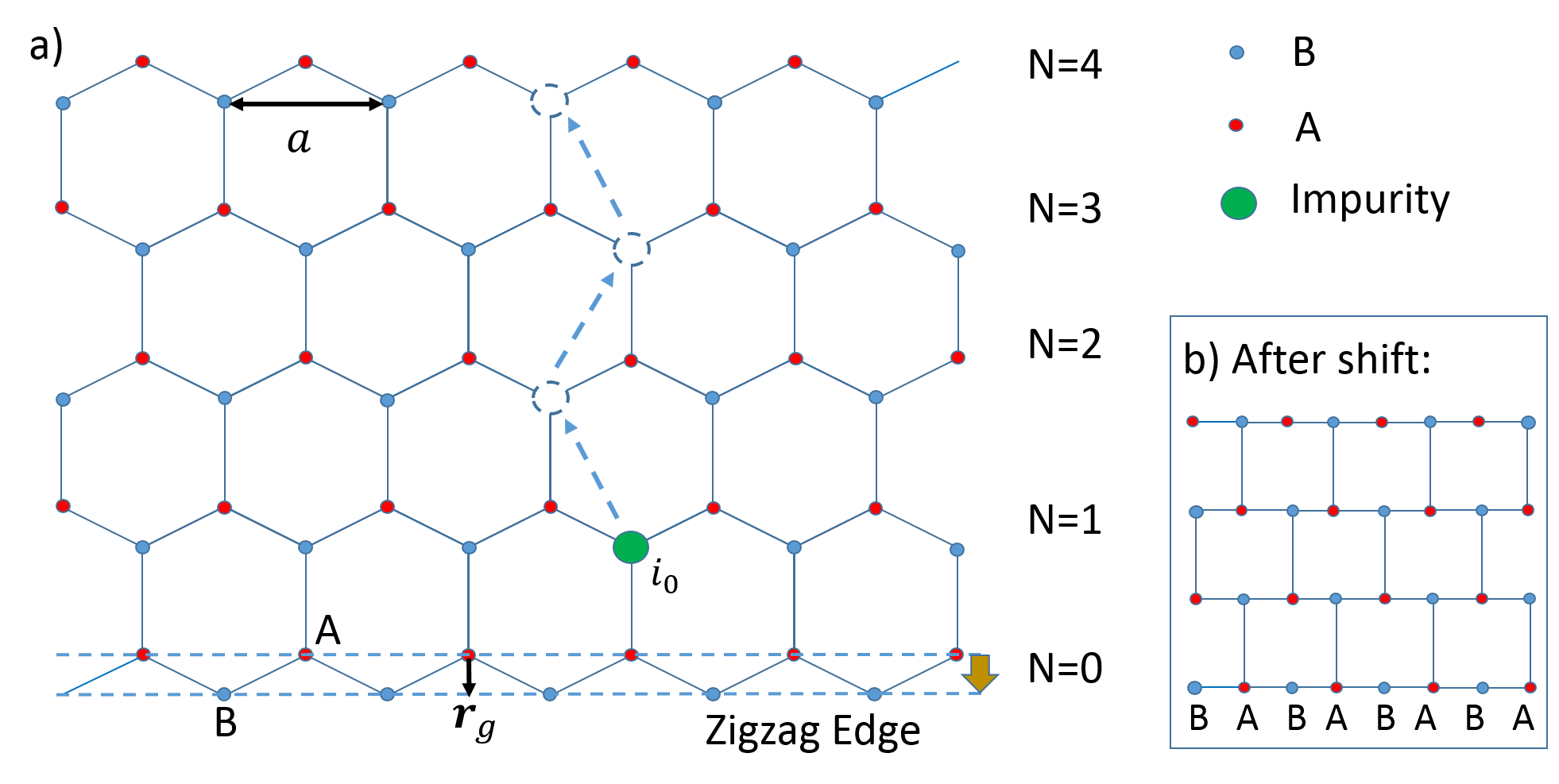
Figure 1: (Color online) Sketch of (a) the zigzag edge with a single impurity at the edge and (b) the “brick wall” lattice to which it maps.

After identifying the boundary conditions, we proceed to solve the 1D Schrödinger equation:

$$\mathcal{H}_{0}^{s}(\alpha,\hat{\beta})\Phi_{s}(k_{x},y)=\epsilon\Phi_{s}(k_{x},y),$$ (7)

where we have used the following notation: $\hat{\beta}=-i\frac{\sqrt{3}a}{2}\partial_{y}$ and $\mathcal{H}_{0}^{s}=\sum_{i}d_{s}^{i}\sigma^{i}$, with

$$d_{s}^{x} = -t(2\cos\alpha+\cos\hat{\beta}),$$

$$d_{s}^{y} = -t\sin\hat{\beta},$$ (8)

$$d_{s}^{z} = s\lambda_{\mathrm{SO}}(2\sin 2\alpha-4\sin\alpha\cos\hat{\beta}),$$

respectively ($\alpha=k_{x}a/2$). The Pauli matrices $\sigma^{i}$ ($i=x,y,z$) is in the pseudo-spin space corresponding to the sublattice $\left(B,A\right)$ components. Furthermore, since $s^{z}$ is a good quantum number, $s=\pm 1$. Below, we look for solutions that are combinations of plane waves $e^{ik_{y}y}$.

We are not interested in finite size effects and therefore take $L\to\infty$. In this limit, the coupling between the two edges vanishes and we obtain the dispersion for the edge states (see Appendix):

$$\epsilon_{s}(k_{x})=\pm\frac{6s\lambda_{\mathrm{SO}}t\sin(k_{x}a)}{\sqrt{t^{2}+\left[4\lambda_{\mathrm{SO}}\sin(k_{x}a/2)\right]^{2}}},$$ (9)

where the $+$ ($-$) sign corresponds to the bottom (top) edge at $y=-L/2$ ($y=+L/2$) and $s=\pm 1$. The bands of edge states cross at $k_{x}=\tfrac{\pi}{a}$ Kane20051prl (for a bearded edge they cross at $k_{x}=0$ Zhang2014Nano , see appendix). For $k_{x}\approx\tfrac{\pi}{a}$, Eq. (9) agrees with the semi-analytic results of Ref. Doh20141arxiv, . For the bottom edge states, below we use the notation $|k_{x},s\rangle$. A plot of the bands Kane20051prl for a wide zigzag ribbon and the corresponding wavefunctions can be found in the Appendix.

III.2 Effect of the magnetic impurity

In order to investigate the effect of the impurity on the electronic transport, we next solve the Lippmann-Schwinger equation (LSE):

$$\left|\Psi\right\rangle=\left|\Phi\right\rangle+{G}_{0}\left(\epsilon\right)\mathcal{V}_{\text{imp}}\left|\Psi\right\rangle,$$ (10)

where ${G}_{0}\left(\epsilon\right)=(\epsilon+i0^{+}-H_{0})^{-1}$ is the Green’s function for Eq. (2). We assume the magnetic impurity to be located on the B sublattice at the bottom edge since the wavefunction of edge states on this edge is mostly localized on the B sublattice (See appendix). In order to extract the transmission and reflection coefficients of the edge electrons, we assume the incident electron has a Bloch wave number $k_{x}^{0}$ on the right-moving edge channel, i.e. $\left|\Phi\right\rangle=\left|k_{x}^{0},s=-1\right\rangle$. Therefore, its energy is $\epsilon_{-}(k_{x}^{0})$ and its group velocity is $v=\partial_{k_{x}}\epsilon_{-}(k_{x})|_{k_{x}=k_{x}^{0}}$. Let us introduce

$$\Phi(s\sigma,\mathbf{r}) =\left\langle s,\sigma,\mathbf{r}\right.\left|\Phi\right\rangle,$$ (11)

$$\Psi(s\sigma,\mathbf{r}) =\left\langle s,\sigma,\mathbf{r}\right.\left|\Psi\right\rangle,$$ (12)

where $\sigma=(+,-)$ corresponds to the $(B,A)$ sublattice. Thus, the asymptotic behavior of the wave function becomes

$$|\Psi\rangle \rightarrow (1+\zeta_{t})|\Phi\rangle~{}~{}{\rm for}~{}~{}x\rightarrow+\infty,$$ (13)

$$|\Psi\rangle \rightarrow |\Phi\rangle+\zeta_{r}|\tilde{\Phi}\rangle~{}~{}{\rm for}~{}~{}x\rightarrow-\infty,$$ (14)

where $|\tilde{\Phi}\rangle=\left|\frac{2\pi}{a}-k_{x}^{0},s=+1\right\rangle$, and

$$\zeta_{t} =-i\lambda_{\text{imp}}L_{x}\frac{\Psi(++,\mathbf{r}_{0})\Phi^{\ast}(-+,\mathbf{r}_{0})}{v},$$ (15)

$$\zeta_{r} =-i\lambda_{\text{imp}}L_{x}\frac{\Psi(-+,\mathbf{r}_{0})\tilde{\Phi}^{\ast}(++,\mathbf{r}_{0})}{v}.$$ (16)

Here $L_{x}$ is the normalization length of system along the edge and $\mathbf{r}_{0}\propto\textbf{R}_{i_{0}}$ is the impurity position.

From the above results, the transmission and the reflection coefficients are obtained from $\zeta_{r}$ as follows:

$$\mathscr{T}(\epsilon) =\left|1+\zeta_{t}\right|^{2}$$ (17)

$$\mathscr{R}(\epsilon) =\left|\zeta_{r}\right|^{2}.$$ (18)

The energy dependence of the transmission coefficient is shown in Fig. 2. Note that, when the magnetic impurity is located on the first atomic row (i.e. $N=1$), the transmission coefficient is essentially energy independent, which makes it similar to a BS impurity in a purely 1D channel. This behavior arises from weak coupling between the edge and bulk states via the impurity (owing to the small weight of the bulk states on the $N=1$ row). This holds true even for relatively large values of $\lambda_{\mathrm{imp}}$. Thus, scattering is dominated by the 1D edge states. However, we believe this behavior is not a robust feature but a peculiarity of present KM model. On the other hand, for the second atomic row and beyond (i.e. $N\geq 2$), the weight of the bulk states is larger, and a strong impurity can thus lead to a sizable coupling between bulk and edge states. As a consequence, for large values of $\lambda_{\mathrm{imp}}$, a pair of narrow scattering anti-resonances appears within the energy gap. In the neighborhood of the anti-resonances, the transmission coefficient changes very rapidly with energy and, on resonance, it vanishes for large $\lambda_{\mathrm{imp}}$.

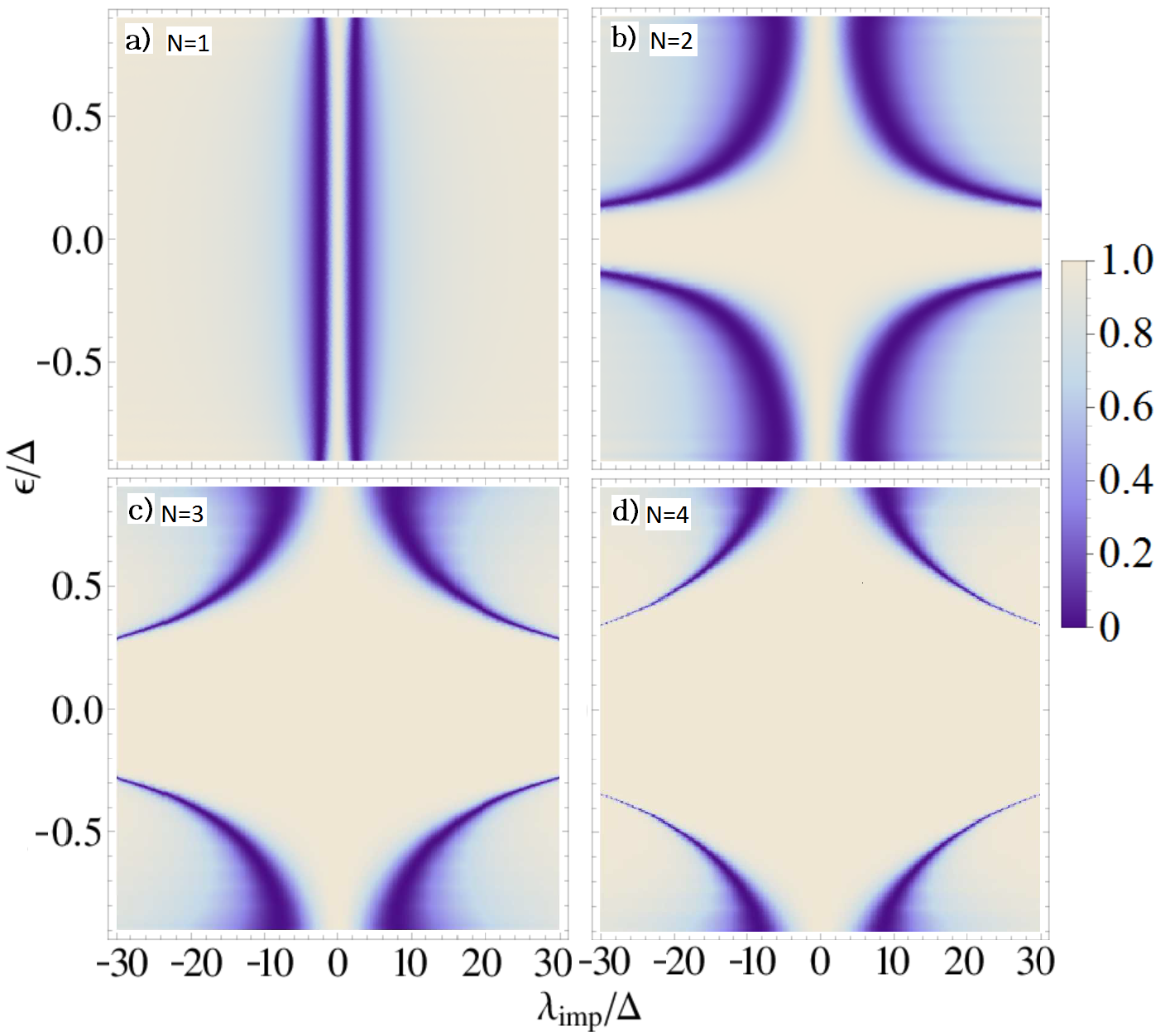
Figure 2: Transmission coefficient $\mathscr{T}(\epsilon)$ for an impurity on a B sublattice site on (a) the first atomic row (i.e. $N=1$), (b) $N=2$, (c) $N=3$, and (d) $N=4$. The spin-orbit coupling is $\lambda_{\mathrm{SO}}=0.06\,t$.

In order to understand the emergence of the pair of scattering anti-resonances, we need to consider the poles of the T-matrix,

$$T(\epsilon)=\left[\bm{1}-\mathcal{V}_{\mathrm{imp}}G_{0}(\epsilon)\right]^{-1}\mathcal{V}_{\mathrm{imp}}$$ (19)

For a strong impurity potential located within the bulk, of the QSHI, the poles of the T-matrix are obtained from the condition

$$\mathrm{det}\left[\bm{1}-\lambda_{\text{imp}}G_{0}^{B}\left(\mathbf{r}_{0},\mathbf{r}_{0},\epsilon\right)s^{x}\right]=0$$ (20)

where $G_{0}^{B}$ is the Green’s function constructed from bulk states. The latter is real for $\epsilon$ within the energy gap since the density of states vanishes there and it is odd in $\epsilon$ (due to the particle-hole symmetry of $H_{0}$), therefore vanishing at $\epsilon=0$, i.e. the middle of the gap. Thus, $G_{0}^{B}\left(\mathbf{r}_{0},\mathbf{r}_{0},\epsilon\right)\propto\epsilon$ for small $\epsilon$. Hence, at large $\lambda_{\mathrm{imp}}$, two bound in-gap states appear at $\epsilon\propto\pm t^{2}/\lambda_{\mathrm{imp}}$, corresponding to the two eigenvalues of $s^{x}$. As the impurity location is shifted towards the edge, the bound states hybridize with the continuum of edge states, leading to the anti-resonances in the transmission coefficient. We will generalize this argument below in section IV.3 when discussing the effect of extensions to the present toy model.

IV 1D effective model

IV.1 Non-interacting limit

After finding a non-perturbative solution to the scattering problem of the edge electrons with a magnetic dopant impurity, in this section we construct a 1D low-energy effective model that describes a non-interacting edge channel in the presence of magnetic impurity at large $\lambda_{\mathrm{imp}}/\Delta$, where $\Delta=3\sqrt{3}\lambda_{\mathrm{SO}}$ ($2\Delta$ is the bulk band gap). The effective model is valid at energies and temperatures smaller than $\Delta$ and therefore only involves the degrees of freedom of the 1D edge and the in-gap states.

The Hamiltonian of the effective 1D model describing the coupling between the edge electrons and the in-gap states is constrained by the existence of a number of symmetries of $H=H_{0}+\mathcal{V}_{\mathrm{imp}}$. The KM model in the ribbon geometry described by $H_{0}$ (cf. Eq. 2), is invariant under TRS ($\mathcal{T}$), spin rotations about the $z$-axis (i.e. $U_{\theta}=\exp(-i\theta s^{z}/2)$, $U^{-1}_{\theta}H_{0}U_{\theta}=H_{0}$), particle-hole symmetry ($\mathcal{C}$), and lattice translations along the edge direction. The impurity potential, $\mathcal{V}_{\text{imp}}$, breaks all those symmetries, but the composite system described by $H=H_{0}+\mathcal{V}_{\text{imp}}$ is invariant under the subgroup span by the combined $U_{\pi}\mathcal{T}$ and $\mathcal{C}\mathcal{T}$ transformations. Therefore, according to the above discussion, the effective model takes the form of a generalized Fano model Fano , describing two discrete levels coupled to the continuum of edge states. Furthermore, this model is invariant under $U_{\pi}\mathcal{T}$ and $\mathcal{C}\mathcal{T}$. Since for $|\lambda_{\mathrm{imp}}|\to\infty$ the position of the resonances approaches the center of the band gap at $\epsilon=0$, we shall focus in the neighborhood of $k_{x}=\frac{\pi}{a}$, where linearization of the edge state spectrum, i.e. $\epsilon_{\pm}(k_{x})=\mp v_{F}k$, is a good approximation. Thus, the effective Hamiltonian can be written as follows:

$${H}_{\mathrm{eff}} =H_{B}+H_{+}\left[u,t_{+}\psi(0)\right]+H_{-}\left[d,t_{-}\psi(0)\right],$$ (21)

$$H_{B} =iv_{F}\int dx\>\psi^{\dagger}s^{z}\partial_{x}\psi+V_{B}a_{0}\psi^{\dagger}(0)s^{x}\psi(0),$$ (22)

$$H_{\pm} [f,\chi]=\pm\epsilon_{0}\>\left(f^{{\dagger}}f-\tfrac{1}{2}\right)+V_{c}a^{1/2}_{0}\left[f^{\dagger}\chi+\mathrm{h.c.}\right]$$ (23)

where $\psi^{{\dagger}}(x)=\left(\psi_{L}^{\dagger}(x),\psi^{\dagger}_{R}(x)\right)$ is the spinor field operator describing the edge states, $u^{{\dagger}}$ and $d^{{\dagger}}$ are the creation operators of electrons in the bound states with $s^{x}$ eigenvalue and energy $s^{x}=+1,\epsilon=+\epsilon_{0}$ and $s^{x}=-1,\epsilon=-\epsilon_{0}$, respectively, and $t_{\pm}=(\pm 1,1)$; $a_{0}=v_{F}/\Delta$ is a short distance cut-off. In the above model, $V_{B}$ describes a renormalized backscattering amplitude for the edge electrons, and $V_{c}$ the tunneling into and out of the bound states. The reflection coefficient for the effective 1D model reads:

$$\mathscr{R}(\epsilon)=\left|\sum_{p=\pm 1}\frac{p}{\frac{iV_{c}^{2}}{(\epsilon+p\epsilon_{0})\Delta}+(1-p\frac{iV_{B}}{2\Delta})}\right|^{2},$$ (24)

which accurately fits the results obtained (numerically) for $\mathcal{T}(\epsilon)=1-\mathscr{R}(\epsilon)$ from the non-perturbative solution of the scattering problem. The left panel of Fig. 3 shows the quality of fit of the transmission coefficient as a function of energy for a magnetic dopant impurity located in the second atomic row (i.e. $N=2$). The behavior of the fitted parameters $V_{c}$, $V_{B}$, and $\epsilon_{0}$ as functions of the impurity potential strength $\lambda_{\mathrm{imp}}$ is shown on the right panel. As expected from the above discussion, $\epsilon_{0}$ decreases as $\lambda_{\mathrm{imp}}\to+\infty$. Note that $V_{c},V_{B}\ll\Delta$, which is consistent with the assumption that the 1D model, Eq. (21) describes only the edge and in-gap states.

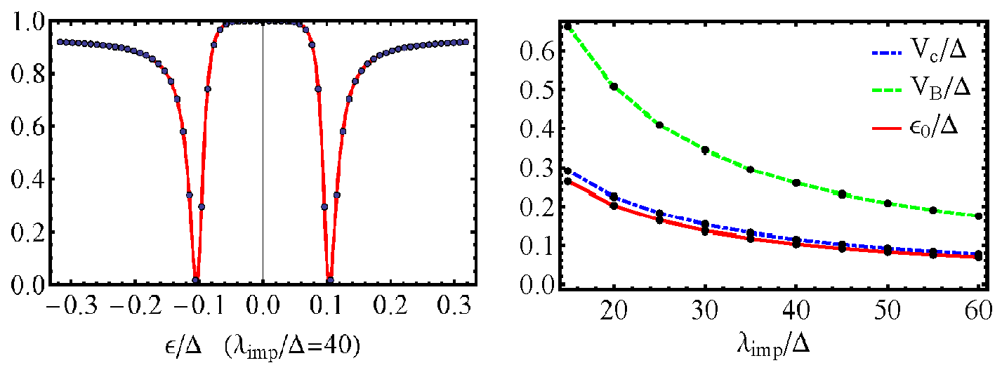
Figure 3: (Color online) (Left) Transmission coefficient for an impurity strength $\lambda_{\mathrm{imp}}=40\>\Delta$ ($\Delta$ is the band gap). Dots are the transmission coefficient obtained numerically for the Kane-Mele model with a backscatterer at the edge. The red line is the fit to the effective model (cf. Eq. 21). (Right) Effective model parameters as a function of $\lambda_{\mathrm{imp}}$.

IV.2 Interaction effects

Finally, we study the effect of electron interactions on the transport properties of the QSHI with a magnetic dopant. Interactions are treated non-perturbatively using the bosonization method Giamarchi . Their characteristic energy scale is $\sim e^{2}/a_{0}$ (where $e$ is the electron charge), which is assumed to be smaller than the band gap, $2\Delta$.

In order to apply bosonization to the interacting model, we further project the effective 1D model in Eq. (21) onto the subspace of excitations with in the neighborhood of the Fermi energy, $\epsilon_{F}$. In particular, when $\epsilon_{F}$ is away from $\pm\epsilon_{0}$, the bound states can be integrated out. To leading order, this yields a renormalized backscattering amplitude

$$V^{\prime}_{B}\simeq V_{B}-\left[\frac{V^{2}_{c}}{\epsilon_{0}-\epsilon_{F}}+\frac{V^{2}_{c}}{\epsilon_{0}+\epsilon_{F}}\right].$$ (25)

and thus the 1D model reduces to the impurity model in a 1D interacting channel studied by Kane and Fisher kane1992prl ; FisherGlazman (cf. $H_{KF}$ in Eq. 27 below) with an impurity potential whose backscattering amplitude $V_{B}=V^{\prime}_{B}$.

On the other hand, on resonance, i.e. for $\epsilon_{F}\simeq+\epsilon_{0}$ ($\epsilon_{F}\simeq-\epsilon_{0}$), we can integrate out only the non-resonant level at $\epsilon_{F}\simeq-\epsilon_{0}$ ($\epsilon_{F}\simeq+\epsilon_{0}$). Assuming (without loss of generality) that $\epsilon_{F}\simeq-\epsilon_{0}$ yields the following low-energy effective model:

$$H^{\prime}_{\mathrm{eff}}=H_{KF}+H_{-}[d,t_{-}\psi(0)]+\left(d^{{\dagger}}d-\tfrac{1}{2}\right)$$

$$\qquad\qquad\times\left[U_{F}\>\psi^{{\dagger}}(0)\psi(0)+U_{B}\>\psi^{{\dagger}}(0)s^{x}\psi(0)\right],$$ (26)

$$H_{KF}=H_{B}+U\int dx\>\rho_{R}\rho_{L}.$$ (27)

The interactions between the edge electrons (with amplitude $U$) and between the edge electrons and the resonant level (with amplitudes $U_{F}$ and $U_{B}$) have been included in the Hamiltonian. We note that integrating out the non-resonant level at $\epsilon=+\epsilon_{0}$ renormalizes the amplitude of $V_{B}-U_{B}/2$ in $H^{\prime}_{\mathrm{eff}}$ by an amount $\simeq V^{2}_{c}/(\epsilon_{F}-\epsilon_{0})\simeq-V^{2}_{c}/2\epsilon_{0}$. In addition, forward scattering is also generated but it is dropped since it can be eliminated by a unitary transformation kane1992prl ; Giamarchi .

The Hamiltonian $H^{\prime}_{\mathrm{eff}}$ in Eqs. (26,27) is akin to a model of a (side-coupled) resonant level in an interacting 1D channel Goldstein2010prlsm ; Lerner . Thus, we apply an analysis similar to the one carried out by Goldstein and Berkovits in Ref. Goldstein2010prlsm to $H^{\prime}_{\mathrm{eff}}$. After bosonizing Giamarchi Eq. (26), we perform a unitary transformation in order to eliminate the forward interaction term $\propto U_{F}$ at the expense of renormalizing the scaling dimension ($\Delta_{c}$) of the operator ($O_{c}\propto V_{c}$) describing the tunneling between the 1D edge channel and the resonant level. Thus,

$$\langle O^{{\dagger}}_{c}(\tau)O_{c}(0)\rangle\sim\frac{V^{2}_{c}}{\tau^{2\Delta_{T}}},$$ (28)

where $\tau$ is the imaginary time and (see Ref. Goldstein2010prlsm and appendix) and

$$\Delta_{T}(K,U_{F})=\tfrac{1}{4}\left[K+K^{-1}\left(1-\tfrac{U_{F}K}{\pi v}\right)^{2}\right].$$ (29)

In this expression

$$K=\sqrt{\frac{2\pi v_{F}-U}{2\pi v_{F}+U}}$$ (30)

is the Luttinger parameter and

$$v=v_{F}\sqrt{1-\left(\frac{U}{2\pi v_{F}}\right)^{2}}$$ (31)

the velocity of the edge plasmons Giamarchi . Hence, tunneling into the resonant level becomes relevant in the renormalization-group (RG) sense for $\Delta_{c}(K,U_{F})<1$. There are two different interaction regimes for which this happens: For repulsive interactions (i.e. $K<1$) and for weak to moderate attraction (i.e. $K\gtrsim 1$). In the former case, both tunneling $V_{c}$ and the BS ($\propto V_{B},U_{F}$) are renormalized to strong coupling by the charge-density wave fluctuations dominant in the 1D channel with $K<1$ Giamarchi . At $T=0$, transmission through the edge channel is completely suppressed. Goldstein2010prlsm ; Lerner

Interestingly, on resonance the transmission through the edge channel of the QHSI is also suppressed for moderately attractive interactions i.e. $K\gtrsim 1$. In this regime, backscattering is naïvely irrelevant kane1992prl and therefore $U_{B}$ is initially suppressed by the dominant superconducting fluctuations in the edge channel (see below). However, the tunneling amplitude $V_{c}$ is still a relevant perturbation since $\Delta_{c}(K,U_{F})<1$. Physically, this is because tunneling is a strongly relevant perturbation in 1D, also in the presence of interactions (see e.g.  Giamarchi , chapter 8).

As the tunneling amplitude renormalizes to strong coupling with decreasing energy scale/temperature, the 2nd order RG flow equations (where $y_{B}\propto U_{B}$, $y_{t}\propto V_{c}$, $\delta_{F}\propto U_{F}$, etc. are dimensionless couplings,m see appendix D for derivation details):

$$\frac{dy_{B}}{d\ln\xi} =\left(1-K\right)y_{B}+y_{t}^{2},$$ (32)

$$\frac{dy_{t}}{d\ln\xi} =\left[1-K/4-(1-\delta_{F})^{2}K^{-1}/4\right]y_{t}$$

$$\qquad+y_{t}(y_{B}+v_{B}),$$ (33)

$$\frac{d\delta_{F}}{d\ln\xi} =4(1-\delta_{F})y^{2}_{t},$$ (34)

$$\frac{dv_{B}}{d\ln\xi} =(1-K)v_{B}.$$ (35)

show that this runaway flow of $y_{t}\propto V_{c}$ drags along both the backscattering amplitude $y_{B}\propto U_{B}$ and $\delta_{F}\propto U_{F}$. This ultimately leads to an effective suppression of the transmission through the edge channel as the temperature (or the energy scale) is reduced Goldstein2010prlsm ; Lerner .

IV.3 Rashba SOC and general magnetic moments

The main results obtained using the toy model introduced above can be easily generalized to account for the Rashba spin-orbit coupling in the band structure, i.e. adding to Eq. (2) a term of the form ($\mathbf{d}_{ij}$ is the vector joining the two nearest neighbor sites $i$ and $j$ on the honeycomb lattice):

$$H_{R}=i\lambda_{r}\sum_{\langle i,j\rangle}c_{i}^{\dagger}(\mathbf{s}\times\mathbf{d}_{ij})c_{j}$$ (36)

and to the case of a more general coupling to the magnetic impurity ($\mathbf{n}$ is a unit vector):

$$\mathcal{\bar{V}}_{\mathrm{imp}}=\lambda_{\mathrm{imp}}c^{{\dagger}}_{i_{0}}\left(\mathbf{s}\cdot\mathbf{n}\right)c_{i_{0}}.$$ (37)

In absence of Rashba and for $\mathbf{n}$ perpendicular to the spin-quantization $z$-axis, we can implement rotation along $s_{z}$ direction to change the magnetic moment in Eq. (37) to the form Eq. (1), which maps the problem to the toy model studied above.

The presence in the system of a uniform Rashba SOC, Eq. 37, violates the conservation of the total $s_{z}$ as well as the particle-hole symmetry of the model. Yet, for weak to moderate Rashba SOC, the topological phase is stable and exhibits robust helical edge states Kane20051prl . In the following, we prove that in the limit $\lambda_{\text{imp}}\rightarrow\infty$, a magnetic dopant impurity in the bulk still generates in-gap bound states, which can resonate with the edge states when the impurity is located near the boundary of the insulator.

For an arbitrary orientation of the magnetic dopant in the bulk of a QSHI, the positions of bound states are determined by the equation (see Eq. (19)):

$$\mathrm{det}\left[\bm{1}-\lambda_{\text{imp}}\left(\mathbf{n}\cdot\mathbf{s}\right)G_{0}^{B}\left(\mathbf{r}_{0},\mathbf{r}_{0},\epsilon\right)\right]=0,$$ (38)

where $G_{0}^{B}(\mathbf{r}_{0},\mathbf{r}_{0},\epsilon)$ is the local Green’s function on the B sublattice, which is a $2\times 2$ matrix in spin space. However, TRS implies that its off-diagonal elements vanish MeirWingreen ; Gurarie $G^{B}_{0,\uparrow\downarrow}\left(\mathbf{r}_{0},\mathbf{r}_{0},\epsilon\right)=G^{B}_{0,\downarrow\uparrow}\left(\mathbf{r}_{0},\mathbf{r}_{0},\epsilon\right)=0$ and $G^{B}_{0,\uparrow\uparrow}\left(\mathbf{r}_{0},\mathbf{r}_{0},\epsilon\right)=G^{B}_{0,\downarrow\downarrow}\left(\mathbf{r}_{0},\mathbf{r}_{0},\epsilon\right)$. Hence, $G_{0}^{B}\left(\mathbf{r}_{0},\mathbf{r}_{0},\epsilon\right)$ is indeed proportional to the unit matrix, i.e.

$$G_{0}^{B}\left(\mathbf{r}_{0},\mathbf{r}_{0},\epsilon\right)=\frac{g_{B}(\epsilon)}{2}\>\bm{1},$$ (39)

where the function $g_{B}(\epsilon)$ is related to the local density of states (LDOS) on the B sublattice. If we apply a rotation to align the spin quantization axis with the direction of $\mathbf{n}$, i.e. $U^{{\dagger}}(\mathbf{n})\left(\mathbf{n}\cdot\mathbf{s}\right)U(\mathbf{n})=s^{z}$, Eq. (38) yields the following conditions for the existence of in-gap bound states:

$$g_{B}(\epsilon)=\pm 2\lambda^{-1}_{\mathrm{imp}}$$ (40)

The function $g_{B}(\epsilon)$ becomes real for $\epsilon$ within the band gap because the LDOS vanishes there. In addition, since the LDOS is positive for $\epsilon$ outside the band gap, Kramers-Kronig relationships imply that $g_{B}(\epsilon)$ must have a zero within the gap, i.e. $g_{B}(\epsilon)=z^{-1}(\epsilon-\epsilon_{c})$, where $z^{-1}$ is the proportionally constant and $\epsilon_{c}$ is an energy within the band gap. For the KM model, particle-hole symmetry further requires that $\epsilon_{c}=0$, which corresponds to the middle of the gap. Rashba SOC breaks particle-hole symmetry and, in general, we expect $\epsilon_{c}\neq 0$. Hence for sufficiently large $\lambda_{\mathrm{imp}}$, the in-gap states will be located at the energies:

$$\epsilon^{\pm}_{0}=\epsilon_{c}\pm\frac{2z}{\lambda_{\mathrm{imp}}}.$$ (41)

However, notice that for $\lambda_{\mathrm{imp}}\sim\Delta$ and/or large particle-hole asymmetry (i.e. $\epsilon_{c}\sim\Delta$), one or both solutions to Eq. (40) may not be real. Indeed, this the case when energy of the in-gap states overlaps with the continuum of states in the conduction or valence bands. However, the above analsys shows that for $\lambda_{\mathrm{imp}}\gg\Delta$, two in-gap states will always be present. The existence of the in-gap bound states can be further explicitly demonstrated by numerically computing the LDOS of QSHI in the presence of the magnetic dopant impurity. Fig. 4 shows the results obtained for the KM with a Rashba SOC of $\lambda_{r}=0.06t$ and $\mathbf{n}$ along the $x$-axis. We have also checked the existence of the in-gap bound state(s) for other choices of $\lambda_{r}$ and $\mathbf{n}$ (not shown here).

As the position of the magnetic impurity is shifted towards the edge, the in-gap states hybridize with the topological edge states, which results in anti-resonances in edge channel transmission. This phenomenon is still described by the generalized Fano model introduced in section III with different energy values for the energy the in-gap state(s) and the tunneling $V_{c}$ treated as an energy dependent function. Nevertheless, provided the Fermi level of the 1D edge ($\epsilon_{F}$) is off resonance, both in-gap states can be integrated out, resulting in a local backscattering potential, which can be treated as a nonmagnetic impurity in an interacting 1D channel Kane20051prl ; Glazman1992 . For $\epsilon_{F}$ on resonance with one of the in-gap state(s), the other non-resonant state can be integrated out, giving rise to the similar model to the one studied at the end of section IV.2, $H^{\prime}_{\mathrm{eff}}$ (cf. Eq. 27, the possible energy dependence of $V_{c}$ being irrelevant in the RG sense). A similar argument applies even when the impurity strength is not weak or the particle-hole symmetry strong, so that only one bound state exists. An exception to the phenomena described the effective model of Eq. (27) is found when there is a symmetry that prevents the hybridization between the in-gap bound states and the electronic states at the edge. Although this is not generic, it is indeed the case for a dopant whose magnetic moment $\mathbf{n}$ points along the spin-quantization axis of the KM, Eq. (2). Thus, the total $s^{z}$ is conserved and the Hilbert space of the problem splits into two subspaces labeled by different $s^{z}$ without any matrix element connecting them. Thus, conservation of total $s^{z}$ prevents the existence of backscattering TanakaFurusakiMateev2011 .

Therefore, although we have based our calculations in a simplified model of the QSHI and the impurity, the phenomena described above does not depend on the specific microscopic details of the model in the large $\lambda_{\text{imp}}$ limit. The emergence of transmission anti-resonances and the interaction induced renormalization of the anti-resonance linewidth Goldstein2010prlsm ; Lerner stems from the coupling between the edge states and the impurity-induced in-gap states. This will generically be present as long as the wave functions of the edge states and the states bound by the magnetic impurity overlap. Similar arguments can be applied to magnetic dopants described by more sophisticated models of of $\mathbb{Z}_{2}$ topological insulators. However, if $\lambda_{\text{imp}}$ is decreased continuously, the bound states will merge into the continuum of bulk states (together or one by one, depending on the degree of particle-hole asymmetry) and finally the resonances will disappear.

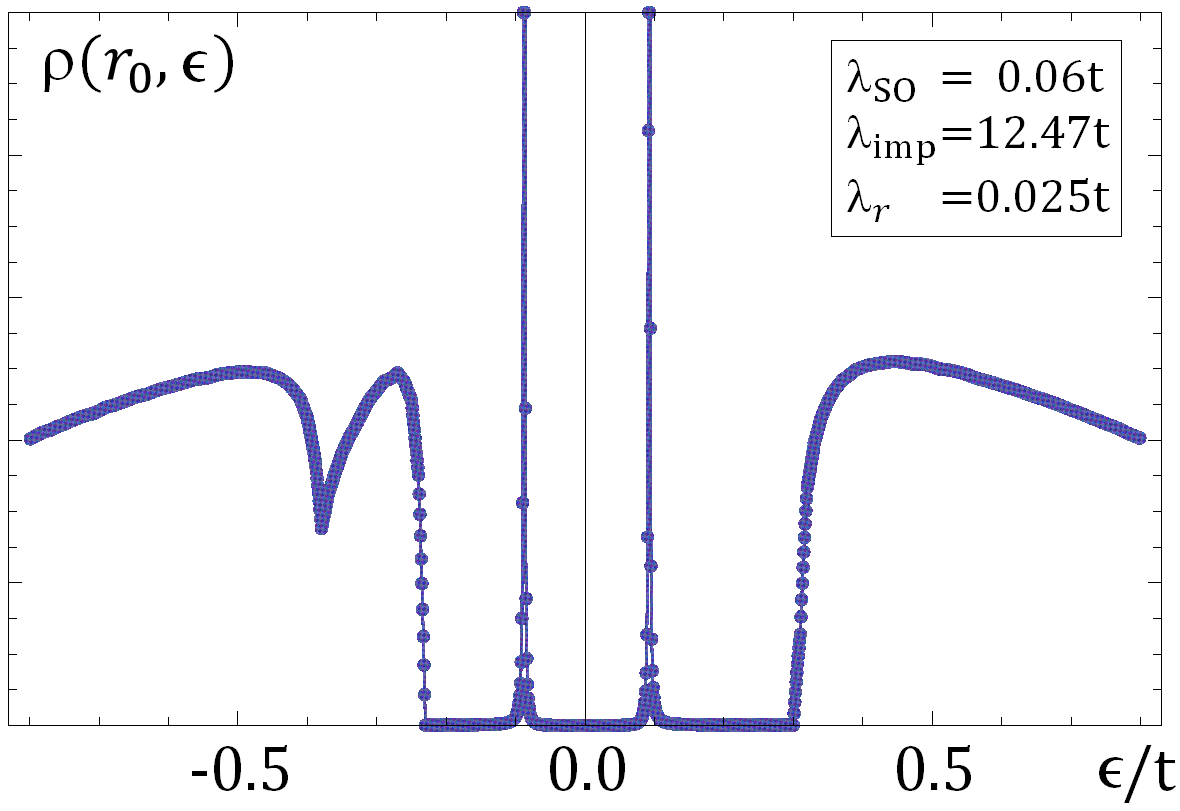
Figure 4: Local density of state at the position of a magnetic dopant impurity located in the bulk of a QSHI insulator described by the Kane-Mele model (see Eqs.2 and 36) with a strength of the bulk Rashba spin-orbit coupling (SOC) $\lambda_{r}=0.06t$. The impurity magnetic moment points along the $x$-axis (see Eq. 1). Notice that the positions of the sharp peaks indicating the existence of impurity-induced in-gap states is not symmetrical with respect to the center of the band gap. This is a consequence of the particle-hole symmetry breaking caused by the Rashba (SOC).

V Summary and Outlook

In summary, we have investigated the transport properties of a quantum spin-Hall insulator in the presence of a strongly coupled magnetic impurity. By obtaining a non-pertubative solution of the scattering problem, we have derived a 1D effective low-energy Hamiltonian describing the system. In the strong coupling limit, the impurity induces in-gap bound state, which in proximity to the edge state broaden into transmission anti-resonances. When the chemical potential of the edge electrons is not resonant with any of the in-gap states induced by the magnetic impurity, the system can be effectively mapped to the problem of a nonmagnetic impurity in a Tomonaga-Luttinger liquid kane1992prl ; matveev1994prb ; FisherGlazman with a renormalized backscattering strength at sufficiently low energy/temperatures (the latter energy scale being set by the separation between the Fermi level and the nearest resonant state). For strong attractive interactions in the channel, this suppression is absent and the 1D channel becomes increasingly transparent at low $T$. On the other hand, when the Fermi energy is on resonance, repulsive and weak to moderately attractive interactions lead to temperature-dependent broadening of the transmission anti-resonance, which effectively suppresses the conductance of the edge channel as the temperature $T$ is decreased.

For many of the current physical realizations of QSHIs exp ; Fei2017np ; Pablo , the regime in which $\lambda_{\mathrm{imp}}\gg\Delta$ is not at all unrealistic as the size of the band gap is typically rather small exp ; review_qshi ; Fei2017np ; Tang ; Pablo , and its size can be tuned close to the topological transition. In addition, in two-dimensional materials, localized moments can appear e.g. from dangling bonds at vacancies vacancy , rather than from magnetic dopants alone. Based on the analysis provided here, we believe that the presence of such localized magnetic defects in proximity to the edge of the recently observed can induce significant backscattering in the newly observed QSHI in the $1$-T^′ phase of WTe₂. The mechanism described here provides additional backscattering sources to accounts for the experimentally observed Fei2017np ; Pablo deviations from conductance quantization at low temperatures. Indeed, if the chemical potential of the edge electrons happens to be at (or near) resonance with in-gap states induced by a magnetic dopant, tunneling in/out of the in-gap states will suppress conductance through the edge channel more effectively than ordinary backscattering (for comparable strength of the bare backscattering $y_{B},v_{B}$ and tunneling $y_{t}$ dimensionless couplings, cf. Eqs. 32 to 35). This is because tunneling in/out of the (nearly resonant) in-gap state is a more relevant perturbation than backscattering, as manifested by its smaller scaling dimension (i.e. typically $\Delta(K,U_{F})<K$, cf. Eq. 29), for both repulsive and moderately attractive interactions. A more detailed analysis relevant to this system will be reported in a future publication. Furthermore, in the future we also plan to study extensions to the model studied here beyond the dilute impurity regime (i.e. the multi-impurity case). Another interesting direction is to treat the spin degrees of the magnetic impurity quantum mechanically. This is especially important to describe spin-$\tfrac{1}{2}$ impurities below the Kondo temperature. Finally, another interesting research direction, relevant to the study of Majorana bound states, is to the study of the competition of the type of magnetic disorder considered here and the proximity to a nearby s-wave superconductor unpub .

We thank L. Glazman, T. Giamarchi, F. Guinea, Y.-H. Ho, C.-L. Huang, and S.-Q. Shen, X.-P. Zhang for useful discussions. M.A.C. gratefully acknowledges support by the Ministry of Science and Technology (Taiwan) under Contract No. 102- 2112-M-007-024-MY5, and Taiwan’s National Center of Theoretical Sciences (NCTS).

Appendix A Spectrum and wavefunctions

Here we provide the analytical approach to solve for the spectrum and the wavefunctions of both bulk and edge states for a generalized Kane-Mele (KM) model Kane20051prl ,

$$\hat{H}_{0}=-t\sum_{\langle i,j\rangle}c_{i}^{{\dagger}}c_{j}-i\lambda_{\mathrm{SO}}\sum_{\langle\langle i,j\rangle\rangle}\nu_{ij}c_{i}^{{\dagger}}s^{z}c_{j}+\lambda_{v}\sum_{i}\xi_{i}c_{i}^{{\dagger}}c_{i}.$$ (42)

where a staggered potential with $\xi_{i}=+1$ for $\mathbf{R}_{i}\in B$ and $\xi_{i}=-1$ for $\mathbf{R}_{i}\in A$ sublattice has been included for generality. As mentioned in the main text, there is a gauge degree of freedom for the Fourier transformation of $\hat{c}^{\dagger}_{i}$ (or $\hat{c}_{i}$) due to the bi-particle structure of the lattice. The gauge freedom allows to effectively shift the lattice yielding different geometries for the edge.

Besides of zigzag edge of interest in the main text, it is also interesting to consider the beard edge in parallel. The correspond to two different gauge choices: 1) Zigzag edge: $\mathbf{r}_{g}=-({a}/{2\sqrt{3}})\mathbf{e}_{y}$ and 2) Beard edge: $\mathbf{r}_{g}=({a}/\sqrt{3})\mathbf{e}_{y}$. In our convention, $\sigma^{z}=\left(+,-\right)$ denotes the sublattice pseudo spin components corresponding to the $\left(B,A\right)$ sublattices.

A.0.1 Spectrum of edge states

For the case with zigzag edge, after the Fourier transformation, we obtain $\mathcal{H}_{0}^{s}(\alpha,\hat{\beta})=\sum_{i}d_{s}^{i}\sigma^{i}$, we have used the notation where Pauli matrices $\sigma^{i}$ ($i=x,y,z$) is in the pseudo-spin space corresponding to the sublattice $\left(B,A\right)$ components of the single-particle spin wave function and

$$d_{s}^{x} =-t(2\cos\alpha+\cos\hat{\beta}),$$ (43)

$$d_{s}^{y} =-t\sin\hat{\beta},$$ (44)

$$d_{s}^{z} =\lambda_{v}+s\lambda_{\mathrm{SO}}(2\sin 2\alpha-4\sin\alpha\cos\hat{\beta}),$$ (45)

with $\alpha=k_{x}a/2$, and $\hat{\beta}=-i\frac{\sqrt{3}a}{2}\partial_{y}$. We set $a=1$ for simplicity. In addition, we treat $\hat{\beta}$ as an operator and $\beta$ as its eigenvalues.

Substituting $\Phi_{s}(k_{x},y)=\chi_{s}e^{\kappa y}$ to Eq. (7), we get the following secular equation:

$$Xf^{2}+Yf+Z=0,$$ (46)

where the variables

$$f \equiv\cosh\frac{\sqrt{3}\kappa}{2},$$ (47)

$$X =-(4\lambda_{\mathrm{SO}}\sin\frac{k_{x}}{2})^{2},$$ (48)

$$Y =8s\lambda_{\mathrm{SO}}\sin\frac{k_{x}}{2}\left(\lambda_{v}+2s\lambda_{\mathrm{SO}}\sin k_{x}\right)-4t^{2}\cos\frac{k_{x}}{2},$$ (49)

$$Z =\epsilon^{2}-t^{2}-4t^{2}(\cos\frac{k_{x}}{2})^{2}-\left(\lambda_{v}+2s\lambda_{\mathrm{SO}}\sin k_{x}\right)^{2}.$$ (50)

Hence, we obtain the following two roots:

$$f_{1,2}=({-Y\pm\sqrt{Y^{2}-4XZ}})/{2X},$$ (51)

Thus, there are four roots for $\kappa$, corresponding to $\pm\kappa_{1,2}$ with $\kappa_{1,2}=\frac{2}{\sqrt{3}}\cosh^{-1}f_{1,2}$. For the edge states, we have that $\mathrm{Re}\>\kappa_{1,2}\neq 0$. Thus, we use the convention that $\mathrm{Re}\>\kappa_{1,2}>0$ for the function $\kappa_{1,2}=\frac{2}{\sqrt{3}}\cosh^{-1}f_{1,2}$.

Note that only two linearly independent wavefunctions satisfy the open boundary conditions corresponding the zigzag edge, namely $\Phi_{s}(k_{x},\pm L/2)=0$ for each value of $\epsilon$. They are

$$g_{c}^{1}(k_{x},y)-g_{c}^{2}(k_{x},y),$$ (52)

$$g_{s}^{1}(k_{x},y)-g_{s}^{2}(k_{x},y),$$ (53)

where Zhou20081prl

$$g_{c}^{i}(k_{x},y) =\frac{\cosh(\kappa_{i}y)}{\cosh(\kappa_{i}L/2)},$$ (54)

$$g_{s}^{i}(k_{x},y) =\frac{\sinh(\kappa_{i}y)}{\sinh(\kappa_{i}L/2)}.$$ (55)

The eigenfunctions can be expressed as the linear combination of the above wavefunctions. By introducing a $2\times 2$ matrix of coefficients $\mathcal{L}=\left[l_{ij}\right]$, the eigenfunctions can be written as follows:

$$\Phi_{s}(k_{x},y)=\mathcal{L}\left[\begin{array}[]{c}g_{c}^{1}(k_{x},y)-g_{c}^{2}(k_{x},y)\\ g_{s}^{1}(k_{x},y)-g_{s}^{2}(k_{x},y)\end{array}\right].$$ (56)

Substituting this function into Eq. (7), and using that $g_{c,s}^{i}$ are linearly independent, we obtain the following conditions relating the column vectors of the matrix $\mathcal{L}$:

$$\mathbf{L}_{2} =\tanh(\kappa_{1}L/2)M_{1}\mathbf{L}_{1},$$ (57)

$$\mathbf{L}_{2} =\tanh(\kappa_{2}L/2)M_{2}\mathbf{L}_{1},$$ (58)

$$\mathbf{L}_{1} =\frac{1}{\tanh(\kappa_{1}L/2)}M_{1}\mathbf{L}_{2},$$ (59)

$$\mathbf{L}_{1} =\frac{1}{\tanh(\kappa_{2}L/2)}M_{2}\mathbf{L}_{2},$$ (60)

where

$$\mathbf{L}_{1} =(l_{11},l_{21})^{T},$$ (61)

$$\mathbf{L}_{2} =(l_{12},l_{22})^{T},$$ (62)

$$M_{i} =\sigma^{y}\left\{\left(-2t\cos\alpha-t\cos\beta_{i}\right)\sigma^{x}\right.$$

$$\qquad\left.+\left(\lambda_{v}+2s\lambda_{\mathrm{SO}}\sin 2\alpha\right.\right.$$

$$\left.\left.\quad-4s\lambda_{\mathrm{SO}}\sin\alpha\cos\beta_{i}\right)\sigma^{z}-\epsilon\right\}/(t\sin\beta_{i}),$$ (63)

$$\beta_{i} =-i\frac{\sqrt{3}}{2}\kappa_{i},$$ (64)

respectively. Note that, in the above derivation, we have used the fact $\cos\hat{\beta}g_{c,s}^{i}(k_{x},y)=\cos\beta_{i}g_{c,s}^{i}(k_{x},y)$, $\sin\hat{\beta}g_{c}^{i}(k_{x},y)=\sin\beta_{i}\tanh(\kappa_{i}L/2)g_{s}^{i}(k_{x},y)$ and $\sin\hat{\beta}g_{s}^{i}(k_{x},y)=\frac{\sin\beta_{i}}{\tanh(\kappa_{i}L/2)}g_{c}^{i}(k_{x},y)$.

The combinations of equations in the same column in Eq.(57) give the secular equation (46), which relates $\kappa_{i}$ and spectrum $\epsilon$. The other two independent equations are obtained by combining diagonal terms in Eq.(57), which yields:

$$\mathbf{L}_{2}=TM_{1}M_{2}\mathbf{L}_{2}=\frac{1}{T}M_{2}M_{1}\mathbf{L}_{2},$$ (65)

where

$$T=\frac{\tanh(\kappa_{1}L/2)}{\tanh(\kappa_{2}L/2)}.$$ (66)

Expressing $\kappa_{i}$ as functions of $\epsilon$, this equation is exactly the constraint for spectrum $\epsilon$. In the following, we will solve this equation. Eq.(65) implies that

$$M_{t}\mathbf{L}_{2}=0,$$ (67)

where $M_{t}\equiv TM_{1}M_{2}-\frac{1}{T}M_{2}M_{1}$. To have a nontrivial solution for $\mathbf{L}_{2}$, the condition $\det M_{t}=0$ is required, which gives

$$(T+\frac{1}{T})^{2}={4D_{0}^{2}}/({{D_{0}^{2}-D_{x}^{2}-D_{y}^{2}-D_{z}^{2}}}),$$ (68)

where

$$D_{x} =t(\cos\beta_{1}-\cos\beta_{2})\epsilon,$$ (69)

$$D_{y} =it(\lambda_{v}+6s\lambda_{\mathrm{SO}}\sin 2\alpha)(\cos\beta_{1}-\cos\beta_{2}),$$ (70)

$$D_{z} =4s\lambda_{\mathrm{SO}}\sin\alpha(\cos\beta_{1}-\cos\beta_{2})\epsilon,$$ (71)

and $D_{0}=t^{2}(2\cos\alpha+\cos\beta_{1})(2\cos\alpha+\cos\beta_{2})+(\lambda_{v}+2s\lambda_{\mathrm{SO}}\sin 2\alpha-4s\lambda_{\mathrm{SO}}\sin\alpha\cos\beta_{1})(\lambda_{v}+2s\lambda_{\mathrm{SO}}\sin 2\alpha-4s\lambda_{\mathrm{SO}}\sin\alpha\cos\beta_{2})-\epsilon^{2}$. For $L\rightarrow\infty$, $T=1$ because $\mathrm{Re}\>\kappa_{1,2}>0$. Thus, it becomes

$$D_{x}^{2}+D_{y}^{2}+D_{z}^{2}=0,$$ (72)

which gives the dispersion

$$\epsilon_{s}^{\pm}=\pm\frac{t(\lambda_{v}+6s\lambda_{\mathrm{SO}}\sin 2\alpha)}{\sqrt{t^{2}+(4\lambda_{\mathrm{SO}}\sin\alpha)^{2}}}.$$ (73)

Note that Eq.(65) gives an additional constraint for the spectra. From $M_{t}\mathbf{L}_{2}=0$ and $T=1$, we obtain

$$(D_{x}\sigma_{x}+D_{y}\sigma_{y}+D_{z}\sigma_{z})\mathbf{L}_{2}=0.$$ (74)

Combining it with $\mathbf{L}_{2}=M_{1}M_{2}\mathbf{L}_{2}$ (Eq.(65)), we obtain the following the constraint:

$$-D_{0}=t^{2}\sin\beta_{1}\sin\beta_{2}.$$ (75)

The second constraint is $\mathrm{Re}\>\kappa_{1,2}>0$. These constraints restrict a region $k_{x}\in\left[\Lambda_{s}^{-},\Lambda_{s}^{+}\right]$, where edge states exist. We show the resulted spectra in Fig. 5.

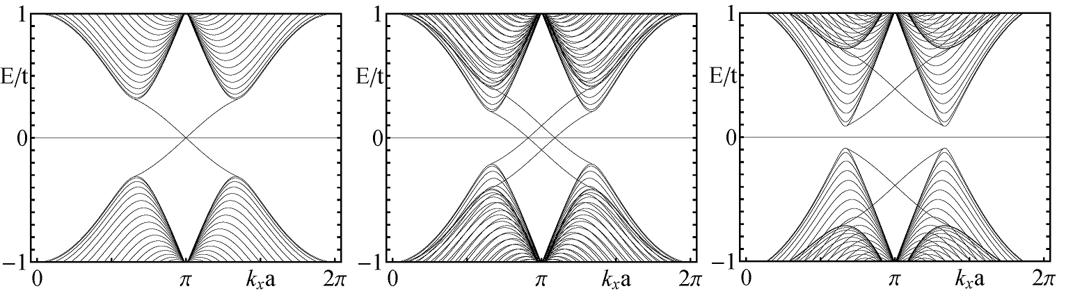
Figure 5: Band structure of a zigzag ribbon described by Eq. (42). Left panel: $\lambda_{\mathrm{SO}}=0.06t$ and $\lambda_{v}=0$; Central panel: $\lambda_{\mathrm{SO}}=0.06t$ and $\lambda_{v}=0.1t<3\sqrt{3}\lambda_{\mathrm{SO}}$; Right panel: $\lambda_{\mathrm{SO}}=0.06t$ and $\lambda_{v}=0.4t>3\sqrt{3}\lambda_{\mathrm{SO}}$.

A.0.2 Wavefunctions for a semi-infinite system

To investigate the wavefunctions at one of edges only, it is helpful to shift the coordinate origin so that the QSHI occupies the upper half plane ($0\leq y\leq L$ with $L\to\infty$). For a semi-infinite system, the wavefunction satisfying the boundary condition $\Phi_{sk_{x}}(0)=\Phi_{sk_{x}}(L\rightarrow\infty)=0$ has a much simpler form:

$$\Phi_{sk_{x}}(y)=C_{s}(k_{x})\chi_{s}(k_{x})(e^{-\kappa_{s,1}y}-e^{-\kappa_{s,2}y}).$$ (76)

Thus, what is left is to determine the $2\times 1$ matrix $\chi_{s}(k_{x})$ and the normalization factor $C_{s}(k_{x})$. For each $k_{x}$, we have obtain the spectra $\epsilon_{s}$ and the wave number $\kappa_{s,i}=\frac{2}{\sqrt{3}}\cosh^{-1}f_{s,i}$ with $i=1,2$ in the last section. Substituting Eq. (76) into the Schrödinger Eq.(7), we obtain

$$\chi_{s}(k_{x})=\Bigg{[}\begin{array}[]{c}-\left[\mathcal{H}_{0}^{s}\right]_{12}/\left\{\left[\mathcal{H}_{0}^{s}\right]_{11}-\epsilon_{s}\right\}\\ 1\end{array}\Bigg{]}\equiv\Bigg{[}\begin{array}[]{c}\chi_{s,1}\\ 1\end{array}\Bigg{]}.$$ (77)

Explicitly,

$$\chi_{s,1}=\frac{2t\cos\frac{k_{x}}{2}+t\exp({\sqrt{3}\kappa_{s,1}}/{2})}{\lambda_{v}+2s\lambda_{\mathrm{SO}}[\sin k_{x}-2\sin({k_{x}}/{2})\cosh({\sqrt{3}\kappa_{s,1}}/{2})]-\epsilon_{s}}$$ (78)

Recall that the above wavefunctions only make sense when evaluated on the discrete set of points of the honeycomb lattice:

$$\psi_{sk_{x}}(n)=C_{s}(k_{x})\chi_{s}(k_{x})(e^{-\kappa_{s,1}ny_{0}}-e^{-\kappa_{s,2}ny_{0}}),$$ (79)

where $y_{0}=\sqrt{3}a/2$. The normalization factor is

$$C_{s}(k_{x})=(1+\left|\chi_{s,1}\right|^{2})^{-1/2}C_{s}^{0}(k_{x})$$ (80)

where

$$C_{s}^{0}(k_{x}) =\left[\Upsilon\left(2\>\mathrm{Re}\>\kappa_{s,1}\right)+\Upsilon\left(2\>\mathrm{Re}\>\kappa_{s,2}\right)\right.$$

$$\left.-\Upsilon\left(\kappa_{s,1}^{\ast}+\kappa_{s,2}\right)-\Upsilon\left(\kappa_{s,1}+\kappa_{s,2}^{\ast}\right)\right]^{-1/2}$$ (81)

and $\Upsilon(k)\equiv{1}/[{1-\exp(-ky_{0})}]$. Upon denoting $\Phi_{sk_{x},\sigma}(\mathbf{r})$ as the $\sigma$ components of $\Phi_{sk_{x}}(\mathbf{r})$, we find $|\Phi_{sk_{x},+}(\mathbf{r})|^{2}\gg|\Phi_{sk_{x},-}(\mathbf{r})|^{2}$ for the case $\lambda_{v}=0$ and $\lambda_{\mathrm{SO}}\ll t$, which suggesting the bottom edge states ‘prefer’ B-sublattice.

A.0.3 Wavefunctions for Bulk States

For the bulk states with periodic boundary conditions, crystal momentum $\mathbf{{k}=(}k_{x},k_{y}\mathbf{)}$ is treated as good quantum number in both the $x$-direction and $y$-direction. Thus, upon setting $\kappa=ik_{y}$ in Eq. (46) (with $\beta=\frac{\sqrt{3}k_{y}}{2}$), we obtain the (bulk) dispersion:

$$E_{s\eta}\left(\mathbf{k}\right)=E_{s\eta}\left(k_{x},k_{y}\right)=\eta\sqrt{t^{2}+4t^{2}\cos\alpha\cos\beta+4t^{2}\cos^{2}\alpha+[\lambda_{v}+2s\lambda_{\mathrm{SO}}(\sin 2\alpha-2\sin\alpha\cos\beta)]^{2}},$$ (82)

where $s,\eta=\pm 1$.

However, for open boundary conditions and in the limit $L\rightarrow\infty$, the spectrum of bulk state is not modified from the above form because the boundary effects become negligible in the thermodynamic limit. On other hand, wavefunctions are modified and become different from Bloch waves because of the scattering with the boundary. Thus, from the secular equation (46), for each $\kappa_{1}=ik_{y}$($k_{y}$ is real) and thus $f_{1}\equiv\cos\frac{\sqrt{3}k_{y}}{2}$, we can find another root, $f_{2}=-\frac{Y}{X}-f_{1}$. In total four different roots for $\kappa$ exist, i.e. $\pm\kappa_{1,2}$ with $\kappa_{1,2}=\frac{2}{\sqrt{3}}\cosh^{-1}f_{1,2}$, corresponding to a same energy $\epsilon$. Note that $f_{1}$ and thus $f_{2}$ are real. Thus there are two different cases: 1) $\left|f_{2}\right|>1$, the plane wave decays at the edge; and 2) $\left|f_{2}\right|\leq 1$, different modes interference with each other:

Case 1: For $\left|f_{2}\right|>1$, we have $\kappa_{2}=\frac{2}{\sqrt{3}}\cosh^{-1}f_{2}$ with $\mathrm{Re}\>\kappa_{2}>0$. Thus the full solutions of the secular equation (46) for $\kappa$ are $\pm ik_{y}$ and $\pm\kappa_{2}$. The mode $\sim e^{\kappa_{2}y}$ diverges for $y\rightarrow\infty$, so it will not emerge and there are only there modes left: $e^{\pm\kappa_{1}y}$ and $e^{-\kappa_{2}y}$. After using the boundary condition $\Phi_{s\eta,\mathbf{k}}(y=0)=0$, only two linear independent wavefunctions are left. The general wavefunction has the following form:

$$\Phi_{s\eta,\mathbf{k}}(y)=\frac{C_{s\eta}(\mathbf{k})}{\sqrt{N_{y}}}\mathcal{L}\Bigg{[}\begin{array}[]{c}\exp(ik_{y}y)-\exp(-\kappa_{2}y)\\ \exp(-ik_{y}y)-\exp(-\kappa_{2}y)\end{array}\Bigg{]},$$ (83)

where $\mathcal{L=}\left[l_{ij}\right]_{2\times 2}$ is a $2\times 2$ matrix, and $C_{s\eta}(\mathbf{k})$ is the normalization constant. Obviously, such a kind of wavefunction is a combination of extended state and local state, which decays at the edge.

Now we need to calculate out the matrix $\mathcal{L}$. Substituting Eq.(83) into Schrödinger equation (7), and using the fact that $\exp(\pm ik_{y}y)$ and $\exp(-\kappa_{2}y)$ are linear independent, we obtain the following results:

$$\mathbf{L}_{1}=c_{1}\Bigg{[}\begin{array}[]{c}l_{1}\\ 1\end{array}\Bigg{]}, ~{}~{}~{}~{}~{}\mathbf{L}_{2}=c_{2}\Bigg{[}\begin{array}[]{c}l_{1}^{\ast}\\ 1\end{array}\Bigg{]},$$ (88)

$$\mathbf{L}_{1}+\mathbf{L}_{2} =\Bigg{[}\begin{array}[]{c}l_{2}\\ 1\end{array}\Bigg{]},$$ (91)

where

$$\mathbf{L}_{1} =(l_{11},l_{21})^{T},$$ (92)

$$\mathbf{L}_{2} =(l_{12},l_{22})^{T},$$ (93)

$$l_{i} =-\frac{\left[\mathcal{H}_{0}^{s}(\alpha,\beta_{i})\right]_{12}}{\left[\mathcal{H}_{0}^{s}(\alpha,\beta_{i})\right]_{11}-E_{s\eta}\left(\mathbf{k}\right)}$$ (94)

and $c_{1}$, $c_{2}$ are constants, $\beta_{1}=\frac{\sqrt{3}}{2}k_{y}$, $\beta_{2}=i\frac{\sqrt{3}}{2}\kappa_{2}$. Solving these equations, we find $c_{1}=\frac{l_{2}-l_{1}^{\ast}}{l_{1}-l_{1}^{\ast}}$ and $c_{2}=\frac{-l_{2}+l_{1}}{l_{1}-l_{1}^{\ast}}$.

The next step is to calculate the normalization coefficient $C_{s\eta}(\mathbf{k})$. For large $L$ limit, $\exp(-\kappa_{2}y)$ does not influence normalization. Using the orthogonality of $\exp(\pm ik_{y}y)$, we obtain

$$C_{s\eta}(\mathbf{k})=\frac{1}{\sqrt{\left|c_{1}\right|^{2}+\left|c_{2}\right|^{2}}\sqrt{\left|l_{1}\right|^{2}+1}}.$$ (95)

As a result, in real space, we have

$$\Phi_{s\eta,\mathbf{k}}(n)=\frac{C_{s\eta}(\mathbf{k})}{\sqrt{N_{y}}}\mathcal{L}\Bigg{[}\begin{array}[]{c}\exp(ik_{y}ny_{0})-\exp(-\kappa_{2}ny_{0})\\ \exp(-ik_{y}ny_{0})-\exp(-\kappa_{2}ny_{0})\end{array}\Bigg{]},$$ (96)

Case 2:   For $\left|f_{2}\right|\leq 1$, we have $\kappa_{2}=\frac{2}{\sqrt{3}}\cosh^{-1}f_{2}=ik_{y}^{\prime}$ with $k_{y}^{\prime}\geq 0$. The full solutions of the secular equation (46) for $\kappa$ are $\pm ik_{y}$ and $\pm ik_{y}^{\prime}$. The boundary conditions $\Phi_{s\eta,\mathbf{k}}(y=0)=0$ require these four running waves inference with each other, and thus there are only three linear independent wavefunctions. Following the method used in previous case, we can construct the eigenfunctions by combining the three wavefunctions. However, we shall proceed in a different way here. Similar to the previous case, there is one eigenfunction,

$$\left|1\right\rangle=\frac{1}{\sqrt{N_{y}}}C_{s\eta}(\mathbf{k})\mathcal{L}\Bigg{[}\begin{array}[]{c}\exp(ik_{y}y)-\exp(-ik_{y}^{\prime}y)\\ \exp(-ik_{y}y)-\exp(-ik_{y}^{\prime}y)\end{array}\Bigg{]},$$ (97)

where $\mathcal{L}$ is same as the one in Eq. (83) except for the replacement of $\kappa_{2}$ with $ik_{y}^{\prime}$ and thus the normalization becomes:

$$C_{s\eta}(\mathbf{k})=\frac{1}{\sqrt{(|c_{1}|^{2}+|c_{2}|^{2})(|l_{1}|^{2}+1)+(|l_{2}|^{2}+1)}}.$$ (98)

The second eigenstate $\left|2\right\rangle$ can be obtained by the replacements: $k_{y}\to k_{y}^{\prime}$ (which implies that $l_{2}\to l_{1}^{\ast}$). We denote the corresponding parameters as $\mathbf{L}_{1}^{\prime}$, $\mathbf{L}_{2}^{\prime}$, $c_{1}^{\prime}$, $c_{2}^{\prime}$ and $C_{s\eta}(\mathbf{k}^{\prime})$. Note that these two eigenstates are not orthogonal.

In the following, we construct an orthogonal and symmetric basis by means of

$$\left|+\right\rangle=\left|1\right\rangle+\vartheta\left|2\right\rangle,~{}~{}~{}~{}\left|-\right\rangle=\left|2\right\rangle+\vartheta\left|1\right\rangle.$$ (99)

Using the orthogonality condition together with $\left\langle 1\right.\left|1\right\rangle=\left\langle 2\right.\left|2\right\rangle=1$, we obtain

$$\left|\vartheta\right|^{2}=1,~{}~{}~{}\text{Re}\>\vartheta=-\text{Re}\>\left\langle 1\right.\left|2\right\rangle,$$ (100)

where $\left\langle 1\right.\left|2\right\rangle=C_{s\eta}(\mathbf{k})C_{s\eta}(\mathbf{k}^{\prime})[-c_{2}^{\ast}(|l_{1}|^{2}+1)-c_{2}^{\prime}(|l_{2}|^{2}+1)]$. We use the convention that $\mathrm{Im}\>\vartheta=\sqrt{1-\left(\mathrm{Re}\>\vartheta\right)^{2}}\geq 0$, and finally, we obtain the orthonormalized wavefunctions

$$\Phi_{s\eta\mathbf{k}}(n) = \frac{1}{\sqrt{2+2\mathrm{Re}d\left[\vartheta\left\langle 1\right.\left|2\right\rangle\right]}}\left|+\right\rangle,$$ (101)

$$\Phi_{s\eta\mathbf{k}^{\prime}}(n) = \frac{1}{\sqrt{2+2\text{Re}\left[\vartheta\left\langle 2\right.\left|1\right\rangle\right]}}\left|-\right\rangle.$$ (102)

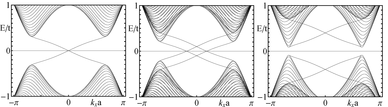
Figure 6: Band structure of a bearded-edge ribbon described by Eq. 42. Left panel: $\lambda_{\mathrm{SO}}=0.06t$ and $\lambda_{v}=0$; Central panel: $\lambda_{\mathrm{SO}}=0.06t$ and $\lambda_{v}=0.1t<3\sqrt{3}\lambda_{\mathrm{SO}}$; Right panel: $\lambda_{\mathrm{SO}}=0.06t$ and $\lambda_{v}=0.4t>3\sqrt{3}\lambda_{\mathrm{SO}}$.

Appendix B Green’s function for the Kane-Mele model in a semi-infinite system

So far, we have obtained the eigenvalues and the complete set of eigenfunctions for the model of Eq. 42. Hence, the Green’s function can be expressed in terms of them:

$$\hat{G}_{0}\left(\epsilon\right)=\sum_{\mathbf{k},s\eta}\frac{\left|\mathbf{k},s,\eta\right\rangle\left\langle\mathbf{k},s,\eta\right|}{\epsilon+i0^{+}-E_{s\eta}(\mathbf{k})}+\sum_{k_{x},s}\frac{\left|k_{x},s\right\rangle\left\langle k_{x},s\right|}{\epsilon+i0^{+}-\epsilon_{s}\left(k_{x}\right)},$$ (103)

where $\left|\mathbf{k},s,\eta\right\rangle=\Phi_{s\eta\mathbf{k}}$. In the real space,

$$G_{0,\sigma\sigma^{\prime}}^{s}\left(\mathbf{r},\mathbf{r}^{\prime},\epsilon\right)=\left\langle\mathbf{r,}s,\sigma\right|\hat{G}_{0}\left(\epsilon\right)\left|\mathbf{r}^{\prime}\mathbf{,}s,\sigma^{\prime}\right\rangle,$$ (104)

where $\sigma=\pm 1$ represents the different components of $\sigma^{z}$. Thus, using $\left\langle\mathbf{r,}s,\sigma\right.\left|\mathbf{k},s,\eta\right\rangle=\Phi_{s\eta\mathbf{k,}\sigma}(\mathbf{r})$ and $\left\langle\mathbf{r,}s,\sigma\right.\left|k_{x},s\right\rangle=\Phi_{sk_{x},\sigma}(\mathbf{r})$, where $\Phi_{s\eta\mathbf{k,}\sigma}(\mathbf{r})$ and $\Phi_{sk_{x},\sigma}(\mathbf{r})$ are the $\sigma$ components of $\Phi_{s\eta\mathbf{k}}(\mathbf{r})$ and $\Phi_{sk_{x}}(\mathbf{r})$ respectively, we have

$$G_{0,\sigma\sigma^{\prime}}^{s}\left(\mathbf{r},\mathbf{r}^{\prime},\epsilon\right) =\sum_{\mathbf{k},\eta}\frac{\Phi_{s\eta\mathbf{k,}\sigma}(\mathbf{r})\Phi_{s\eta\mathbf{k,}\sigma^{\prime}}^{\ast}(\mathbf{r}^{\prime})}{\epsilon+i0^{+}-E_{s\eta}(\mathbf{k})}$$

$$~{}~{}~{}~{}+\sum_{k_{x}}\frac{\Phi_{sk_{x},\sigma}(\mathbf{r})\Phi_{sk_{x},\sigma^{\prime}}^{\ast}(\mathbf{r}^{\prime})}{\epsilon+i0^{+}-\epsilon_{s}\left(k_{x}\right)}.$$ (105)

Appendix C Spectrum of the beard edge

For comparison purposes, we also study the edge spectrum for the beard edge. Using a gauge choice where $\mathbf{r}_{g}=({a}/\sqrt{3})\mathbf{e}_{y}$, and following the same steps as for the zigzag case, we obtain the spectrum for edge state:

$$\epsilon_{s}^{\pm}=\pm\frac{t[2s\lambda_{\mathrm{SO}}\sin\alpha+\cos\alpha(\lambda_{v}+2s\lambda_{\mathrm{SO}}\sin 2\alpha)]}{\sqrt{(t\cos\alpha)^{2}+(2\lambda_{\mathrm{SO}}\sin\alpha)^{2}}}.$$ (106)

In this case, the constraint becomes

$$-D_{0}=4t^{2}\cos^{2}\alpha\sin\beta_{1}\sin\beta_{2},$$ (107)

where

$$D_{0} =t^{2}w_{1}w_{2}+u_{1}u_{2}-\epsilon^{2},$$

$$w_{i} =1+2\cos\alpha\cos\beta_{i},$$

$$u_{i} =\lambda_{v}+2s\lambda_{\mathrm{SO}}\sin 2\alpha-4s\lambda_{\mathrm{SO}}\sin\alpha\cos\beta_{i}.$$ (108)

The resulting band structure is shown in Fig. 6. Note that the edge states intersect at $k_{x}=0$ Zhang2014Nano .

Appendix D Renormalization group analysis

Next, in order to deal with the effects of interactions in a nonperturbative way, we shall rely upon the bosonization technique. The resulting model is analyzed along the lines of the analysis reported is Ref. Goldstein2010prlsm, .

In bosonization the electron field operator for the right ($R$) and left moving ($L$) edge electron can be expressed in terms of a set of bosonic fields $\theta(x)$ and $\phi(x)$ as follows:

$$\psi_{R(L)}\left(x\right)=\frac{U_{R(L)}}{\sqrt{2\pi v\xi}}e^{-i\left[\pm\phi\left(x\right)-\theta\left(x\right)\right]},$$ (109)

where $\xi$ is a short-distance cutoff, $v$ is the plasmon velocity (cf. Eq. 31), $U_{R}$ and $U_{L}$ are the so-called Klein factors satisfying $\left\{U_{r},U_{r^{\prime}}\right\}=2\delta_{r,r^{\prime}}$, which allows to satisfy the anti-commutation relations between the two fermion chiralities $R$ and $L$. The bosonic fields obey

$$\left[\phi\left(x\right),\theta\left(x^{\prime}\right)\right]=i\frac{\pi}{2}\mathrm{sgn}(x^{\prime}-x).$$ (110)

The chiral densities are given by

$$\rho_{R(L)}\left(x\right)=-\frac{1}{2\pi}\left(\partial_{x}\phi\mp\partial_{x}\theta\right).$$ (111)

After bosonizing the low energy effective model and upon applying a unitary transformation generated by

$$S=\exp\left[i\zeta\theta_{0}\right]$$ (112)

with $\zeta=\delta_{F}\left(d^{\dagger}d-\frac{1}{2}\right)$, $\delta_{F}=\tfrac{KU_{F}}{\pi v}$, and using the factor $e^{-i\zeta\theta\left(0\right)}\partial_{x}\phi\left(x\right)e^{i\zeta\theta\left(0\right)}=\partial_{x}\phi\left(x\right)-i\zeta\left[\theta\left(0\right),\partial_{x}\phi\left(x\right)\right]=\partial_{x}\phi\left(x\right)+\zeta\pi\delta\left(x\right)$, the forward scattering term $\propto U_{F}$ can be eliminated from $H^{\prime}_{\mathrm{eff}}$ (cf. Eq. (27)), and the resulting Hamitonian, $H_{\text{eff}}^{\prime\prime}=S^{\dagger}H_{\text{eff}}^{\prime}S$ reads:

$$H_{\text{eff}}^{\prime\prime} =H_{\ast}+\frac{v_{B}}{\xi}\left[U_{R}U_{L}e^{2i\phi_{0}}+U_{L}U_{R}e^{-2i\phi_{0}}\right]$$

$$+\frac{2y_{B}}{\xi}\left(d^{\dagger}d-\frac{1}{2}\right)\left[U_{R}U_{L}e^{2i\phi_{0}}+U_{L}U_{R}e^{-2i\phi_{0}}\right]$$

$$+\frac{y_{t}}{\xi}\left[d^{\dagger}\left(U_{R}e^{-i\left(\phi_{0}-\lambda\theta_{0}\right)}-U_{L}e^{i\left(\phi_{0}+\lambda\theta_{0}\right)}\right)\right.$$

$$\left.+\quad\left(U_{R}e^{i\left(\phi_{0}-\lambda\theta_{0}\right)}-U_{L}e^{-i\left(\phi_{0}+\lambda\theta_{0}\right)}\right)d\right],$$ (113)

where

$$H_{\ast} =\frac{v}{2\pi}\int dx\left[K\left(\partial_{x}\theta\right)^{2}+K^{-1}\left(\partial_{x}\phi\right)^{2}\right]$$

$$\qquad-\varepsilon_{0}\left(d^{\dagger}d-\frac{1}{2}\right).$$ (114)

Here $\varepsilon_{0}$ denotes the distance of the bound state from the Fermi energy of the edge channel, $\epsilon_{F}$. In what follows we focus on the resonant case for which $\epsilon_{0}=0$. In addition, $\lambda=1-\delta_{F}$, $\phi_{0}=\phi(x=0)$, $\theta_{0}=\theta(x=0)$, $v_{B}$, $y_{B}$, $y_{t}$ are dimensionless couplings, and $K$ is the Luttinger parameter and $v$ is the edge plasmon velocity.

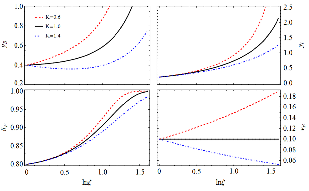
Figure 7: The sketch of the RG flows for the couplings that parametrize the effective low-energy model.

Using Cardy’s approach Cardy and taking into account that

$$\left\langle e^{2i\phi_{0}(\tau)}e^{-2i\phi_{0}(0)}\right\rangle \sim|\tau|^{-2K},$$ (115)

$$\left\langle e^{i[\phi_{0}(\tau)-\lambda\theta_{0}(\tau)]}e^{-i[\phi_{0}(0)-\lambda\theta_{0}(0)]}\right\rangle \sim|\tau|^{-\alpha(K,\lambda)},$$ (116)

$$\alpha(K,\lambda)=\frac{K}{2}+\frac{\lambda^{2}K^{-1}}{2},$$ (117)

we arrive at the set of RG equations valid to second order in the couplings describing backscattering and tunneling in and out of the resonant level given in  (32)-(35). The RG equations are similar to those derived in Ref. Goldstein2010prlsm, for a model of a resonant level that is side-coupled to an interacting 1D electron system. As described in the main text, the equations show that for weak to moderate attractive interactions (i.e. $K\gtrsim 1$), the tunneling operator $\propto y_{t}$ is flows to strong coupling. On the other hand, both the backscattering interaction ($\propto y_{B}$) and potential ($\propto v_{B}$) will be initially suppressed. Eventually, the runaway flow of $y_{t}$ drags along $\delta_{F}$ and $y_{B}$, quickly driving the forward interaction with the level to its fixed point $\delta^{*}_{F}=1$. As a result, the transmission through the impurity will be suppressed, as discussed in the main text.

Fig. 7 shows a sketch of the typical RG flows for moderately repulsive (i.e. $K\lesssim 1$) and moderately attractive (i.e. $K\gtrsim 1$) interactions. In both regimes, alls couplings (execpt for the backscattering potential $v_{B}$ for $K>1$, cf Eq. 35) rapidly reach values of order unity, which in the perturbative approach corresponds to a runaway flow to strong coupling.

References

- (1) M. Z. Hasan and C. L. Kane, Rev. Mod. Phys. 82, 3045 (2010); X.-L. Qi and S.-C. Zhang, Rev. Mod. Phys. 83, 1057 (2011).
- (2) M. König, S. Wiedmann, C. Brüne, A. Roth, H. Buhmann, L. W. Molenkamp, X.-L. Qi, and S.-C. Zhang, Science 318, 766 (2007); A. Roth, C. Brüne, H. Buhmann, L. W. Molenkamp, J. Maciejko, X.-L. Qi, and S.-C. Zhang, Science 325, 294 (2009); K. C. Nowack, E. M. Spanton, M. Baenninger, M. König, J. R. Kirtley, B. Kalisky, C. Ames, P. Leubner, C. Brüne, H. Buhmann, L. W. Molenkamp, D. Goldhaber-Gordon, and K. A. Moler, Nat. Mater. 12, 787 (2013); G. Grabecki, J. Wróbel, M. Czapkiewicz, Ł. Cywiński, S. Gierałtowska, E. Guziewicz, M. Zholudev, V. Gavrilenko, N. N. Mikhailov, S. A. Dvoretski, F. Teppe, W. Knap, and T. Dietl, Phys. Rev. B 88, 165309 (2013); G. M. Gusev, Z. D. Kvon, E. B. Olshanetsky, A. D. Levin, Y. Krupko, J. C. Portal, N. N. Mikhailov, and S. A. Dvoretsky, Phys. Rev. B 89, 125305 (2014); I. Knez, R.-R. Du, and G. Sullivan, Phys. Rev. Lett. 107, 136603 (2011); K. Suzuki, Y. Harada, K. Onomitsu, and K. Muraki, Phys. Rev. B 87, 235311 (2013); I. Knez, C. T. Rettner, S.-H. Yang, S. S. P. Parkin, L. Du, R.-R. Du, and G. Sullivan, Phys. Rev. Lett. 112, 026602 (2014); E. M. Spanton, K. C. Nowack, L. Du, G. Sullivan, R.-R. Du, and K. A. Moler, Phys. Rev. Lett. 113, 026804 (2014).
- (3) G. Dolcetto, M. Sassetti, and T.-L. Schmidt, Rivista del Nuovo Cimento 39, 113 (2016).
- (4) C. Xu and J. E. Moore, Phys. Rev. B 73, 045322 (2006).
- (5) C. Wu, B. A. Bernevig, and S. C. Zhang, Phys. Rev. Lett. 96, 106401 (2006).
- (6) A. Ström, H. Johannesson, and G. I. Japaridze, Phys. Rev. Lett. 104, 256804 (2010).
- (7) C. L. Kane and E. J. Mele, Phys. Rev. Lett. 95, 226801 (2005); Phys. Rev. Lett. 95, 146802 (2005).
- (8) J. Wang, Y. Meir, and Y. Gefen, Phys. Rev. Lett. 118, 046801 (2017).
- (9) A. Amarici, L. Privitera, F. Petocchi, M. Capone, G. Sangiovanni, and B. Trauzettel, Phys. Rev. B 95, 205120 (2017).
- (10) A. F. Young, J. D. Sanchez-Yamagishi, B. Hunt, S. H. Choi, K. Watanabe, T. Taniguchi, R. C. Ashoori, and P. Jarillo-Herrero, Nature 505, 528 (2014).
- (11) F. Yang, L. Miao, Z. F. Wang, M.-Y. Yao, F. Zhu, Y. R. Song, M.-X. Wang, J.-P. Xu, A. V. Fedorov, Z. Sun, G. B. Zhang, C. Liu, F. Liu, D. Qian, C. L. Gao, and J.-F. Jia, Phys. Rev. Lett. 109, 016801 (2012).
- (12) I. K. Drozdov, A. Alexandradinata, S. Jeon, S. Nadj-Perge, H. Ji, R. J. Cava, A. Bernevig, and A. Yazdani, Nat. Phys. 10, 664 (2014).
- (13) X. Qian, J. Liu, L. Fu, and J. Li, Science 346, 1344 (2014).
- (14) Z. Fei, T. Palomaki, S. Wu, W. Zhao, X. Cai, B. Sun, P. Nguyen, J. Finney, X. Xu, and D. H. Cobden, Nat. Phys. 13, 677 (2017).
- (15) S. Tang, C. Zhang, D. Wong, Z. Pedramrazi, H.-Z. Tsai, C. Jia, B. Moritz, M. Claassen, H. Ryu, S. Kahn, J. Jiang, H. Yan, M. Hashimoto, D. Lu, R. G. Moore, C.-C. Hwang, C. Hwang, Z. Hussain, Y. Chen, M. M. Ugeda, Z. Liu, X. Xie, T. P. Devereaux, M. F. Crommie, S.-K. Mo, and Z.-X. Shen, Nat. Phys. 13, 683 (2017).
- (16) S. Wu, V. Fatemi, Q. D. Gibson, K. Watanabe, T. Taniguchi, R. J. Cava, and P. Jarillo-Herrero, Science 359, 76-79 (2018).
- (17) F. Nichele, H. J. Suominen, M. Kjaergaard, C. M. Marcus, E. Sajadi, J. A. Folk, F. Qu, A. J. A. Beukman, F. K. de Vries, J. van Veen, S. Nadj-Perge, L. P Kouwenhoven, B.-M. Nguyen, A. A Kiselev, W. Yi, M. Sokolich, M. J Manfra, E. M Spanton, and K. A. Moler, New J. Phys. 18, 083005 (2016).
- (18) T. Li, P. Wang, H. Fu, L. Du, K. A. Schreiber, X. Mu, X. Liu, G. Sullivan, G. A. Csáthy, X. Lin, and R.-R. Du, Phys. Rev. Lett. 115, 136804 (2015).
- (19) L. Du, ,T. Li, W. Lou, X. Wu, X. Liu, Z. Han, C. Zhang, G. Sullivan, A. Ikhlassi, K. Chang, and R.-R. Du, Phys. Rev. Lett. 119, 056803 (2017).
- (20) T. L. Schmidt, S. Rachel, F. von Oppen, and L. I. Glazman, Phys. Rev. Lett. 108, 156402 (2012).
- (21) J. C. Budich, F. Dolcini, P. Recher, and B. Trauzettel, Phys. Rev. Lett. 108, 086602 (2012).
- (22) N. Lezmy, Y. Oreg, and M. Berkooz, Phys. Rev. B 85, 235304 (2012).
- (23) J. I. Väyrynen, M. Goldstein, and L. I. Glazman, Phys. Rev. Lett. 110, 216402 (2013); J. I. Väyrynen, M. Goldstein, Y. Gefen, and L. I. Glazman, Phys. Rev. B 90, 115309 (2014).
- (24) N. Kainaris, I. V. Gornyi, S. T. Carr, and A. D. Mirlin Phys. Rev. B 90, 075118 (2014).
- (25) F. Crépin, J. C. Budich, F. Dolcini, P. Recher, and B. Trauzettel, Phys. Rev. B 86, 121106 (2012); F. Geissler, F. Crépin, and B. Trauzettel, Phys. Rev. B 89, 235136 (2014).
- (26) L. Kimme, B. Rosenow, and A. Brataas, Phys. Rev. B 93, 081301 (2016).
- (27) M. Kharitonov, F. Geissler, and B. Trauzettel Phys. Rev. B 96, 155134 (2017).
- (28) Y. Tanaka, A. Furusaki, and K. A. Matveev, Phys. Rev. Lett. 106, 236402 (2011).
- (29) Q. Liu, C.-X. Liu, C. Xu, X.-L. Qi, and S.-C. Zhang, Phys. Rev. Lett. 102, 156603 (2009); R. Z̆itko, Phys. Rev. B 81, 241414 (R) (2010); H.-M. Guo and M. Franz, Phys. Rev. B 81, 041102 (R) (2010).
- (30) E. Eriksson, A. Ström, G. Sharma, and H. Johannesson Phys. Rev. B 86, 161103(R) (2012).
- (31) J. Maciejko, C. Liu, Y. Oreg, X.-L. Qi, C. Wu, S.-C. Zhang, Phys. Rev. Lett. 102, 256803 (2009).
- (32) J. S. Van Dyke and D. K. Morr, Phys. Rev. B 93, 081401(R) (2016).
- (33) J. S. Van Dyke and D. K. Morr, Phys. Rev. B 95, 045151 (2017).
- (34) U. Fano, Phys. Rev. 124, pp. 1866 (1961).
- (35) J. R. Schieffer, Journal of Applied Physics 38, 1143 (1967).
- (36) C. L. Kane and M. P. A. Fisher, Phys. Rev. Lett. 68, 1220 (1992); Phys. Rev. B 46, 15233 (1992).
- (37) D. Yue, L. I. Glazman and K. A. Matveev, Phys. Rev. B 49, 1966 (1994).
- (38) M. P. A. Fisher and L. Glazman in “Mesoscopic Electron Transport”, edited by L. Kowenhoven, G. Schön and L. Sohn, NATO ASI Series E, Kluwer Academic Publishers (Dordrecht, The Netherlands) (1997).
- (39) L. I. Glazman, I. M. Ruzin, and B. I. Shklovskii, Phys. Rev. B 45, 8454 (1992).
- (40) S.-J. Qin, M. Fabrizio, and L. Yu, Phys. Rev. B 54, R9643(R) (1996).
- (41) C. Rylands and N. Andrei, Phys. Rev. B 94, 115142 (2016).
- (42) Z. Yao, H. W. Ch. Postma, L. Balents, and C. Dekker, Nature (London) Nature 402, 273-276 (1999).
- (43) A. O. Gogolin, A. A. Nersesyan, and A. M. Tsvelik, Bosonization and Strongly Correlated Systems Cambridge Univeristy Press (Cambridge, UK 1999). T. Giamarchi, Quantum Physics in One-dimension, Clarendon Press (Oxford, UK 2004).
- (44) R. R. Nair, I.-L. Tsai, M. Sepioni, O. Lehtinen, J. Keinonen, A. V. Krasheninnikov, A. H. Castro Neto, M. I. Katsnelson, A. K. Geim, and I. V. Grigorieva, Nat. Comm. 4, 2010 (2010); M. A. Khan, M. Erementchouk, J. Hendrickson, and M. N. Leuenberger, Phys. Rev. B 95, 245435 (2017).
- (45) B. Zhou, H.-Z. Lu, R.-L. Chu, S.-Q. Shen, and Q. Niu, Phys. Rev. Lett. 101, 246807 (2008).
- (46) G. Zhang, X. Li, G. Wu, J. Wang, D. Culcer, E. Kaxiras, and Z. Zhang, Nanoscale 6, 3259 (2014).
- (47) H. Doh, G. S. Jeon, and H. J. Choi, ArXiv:1408.4507 (2014).
- (48) M. Goldstein and R. Berkovits, Phys. Rev. Lett. 104, 106403 (2010).
- (49) I. V. Lerner, V. I. Yudson, and I. V. Yurkevich, Phys. Rev. Lett. 100, 256805 (2008).
- (50) Y. Meir and N. S. Wingreen, Phys. Rev. B 50, 4947(R) (1994).
- (51) V. Gurarie, Phys. Rev. B 83, 085426 (2011).
- (52) M. A. Cazalilla and J.-H. Zheng, in preparation.
- (53) J. Cardy, Scaling and Renormalization in Statistical Physics, Cambridge University Press (Cambrdige, UK, 1996).