Statistical state dynamics based theory for the formation and equilibration of Saturn’s north polar jet

Abstract

Coherent jets containing most of the kinetic energy of the flow are a common feature in observations of atmospheric turbulence at planetary scale. In the gaseous planets these jets are embedded in a field of incoherent turbulence on scales small relative to the jet scale. Large scale coherent waves are sometimes observed to coexist with the coherent jets and the incoherent turbulence with a prominent example of this phenomenon being the distortion of Saturn’s North Polar Jet (NPJ) into a distinct hexagonal form. Observations of this large scale jet-wave-turbulence coexistence regime raises the question of identifying the mechanism responsible for forming and maintaining this turbulent state. The coherent planetary scale jet component of the turbulence arises and is maintained by interaction with the incoherent small-scale turbulence component. It follows that theoretical understanding of the dynamics of the jet-wave-turbulence coexistence regime can be facilitated by employing a statistical state dynamics (SSD) model in which the interaction between coherent and incoherent components is explicitly represented. In this work, a two-layer beta-plane SSD model closed at second order is used to develop a theory that accounts for the structure and dynamics of the NPJ. An asymptotic analysis is performed of the SSD equilibrium in the weak jet damping limit that predicts a universal jet structure in agreement with observations of the NPJ. This asymptotic theory also predicts the wavenumber (six) of the prominent jet perturbation. Analysis of the jet-wave-turbulence regime dynamics using this SSD model reveals that jet formation is controlled by the effective value of $\beta$ and the required value of this parameter for correspondence with observation is obtained. As this is a robust prediction it is taken as an indirect observation of a deep poleward sloping stable layer beneath the NPJ. The slope required is obtained from observations of the magnitude of the zonal wind component of the NPJ. The amplitude of the wave six perturbation then allows identification of the effective turbulence excitation maintaining this combined structure. The observed jet structure is then predicted by the theory as is the wave six disturbance. The wave six perturbation, which is identified as the least stable mode of the equilibrated jet, is shown to be primarily responsible for equilibrating the jet with the observed structure and amplitude.

I Introduction

Coherent structures emergent from small scale turbulence are often observed in planetary atmospheres with the zonal jets of the gaseous planets being familiar examples (Ingersoll, 1990; Vasavada and Showman, 2005; Sánchez-Lavega et al., 2000; Galperin et al., 2014). While this phenomenon of spontaneous large scale jet organization from small scale turbulence has been extensively investigated in both observational and theoretical studies (Kraichnan, 1967; Rhines, 1975; Williams, 1979, 2003; Panetta, 1993; Nozawa and Yoden, 1997; Huang and Robinson, 1998; Lee, 2005; Manfroi and Young, 1999; Vallis and Maltrud, 1993; Cho and Polvani, 1996; Read et al., 2004; Showman, 2007; Scott and Polvani, 2008; Galperin et al., 2004) the physical mechanism underlying it remains controversial. The prominence of jets in planetary turbulence is in part due to the jet being a nonlinear stationary solution of the dynamics in the limit of vanishing dissipation and therefore not disrupted by nonlinear advection on the time scale of the large scale shear. However, its being a stationary solution is insufficient by itself to serve as an explanation for the observed jets for three reasons. First, strong jets typically assume a characteristic structure for a given set of system parameters, while any zonally symmetric flow is a fixed point of the inviscid dynamics. Second, nonlinear stationary states lack a mechanism of maintenance against dissipation and so can not explain the fact that the observed jets, which are not maintained by coherent external forcing such as by an imposed pressure gradient, persist much longer than the dissipation time scale. Third, planetary jets commonly appear to be unstable; for example, the north polar jet (NPJ) of Saturn robustly satisfies the Rayleigh–Kuo necessary condition for barotropic instability in a dissipationless stationary flow (Antuñano et al., 2015; Sánchez-Lavega et al., 2014), and barotropic instability of this jet has been verified by eigenanalysis (Barbosa Aguiar et al., 2010).

The aforementioned considerations imply that a comprehensive theory for the existence of large scale jets in the atmospheres of the gaseous planets and in particular Saturn’s NPJ must provide a mechanism for the formation and maintenance of the jet from incoherent turbulence, the particular structure assumed by the jet and its stability. In addition to these the case of the NPJ also requires that the theory account for the prominent coherent wave six perturbation that distorts the jet into a distinct hexagonal form.

The primary mechanism by which the large scale jets of the gaseous planets are maintained is upgradient momentum flux resulting from straining of the perturbation field by the mean jet shear which produces a spectrally nonlocal interaction between the small-scale perturbation field and the large-scale jet. This mechanism has been verified in observational studies of both the Jovian and Saturnian atmospheres (Ingersoll et al., 2004; Salyk et al., 2006; Delgenio et al., 2007), as well as in numerical simulations (Nozawa and Yoden, 1997; Huang and Robinson, 1998; Showman, 2007) and in laboratory experiments (Wordsworth et al., 2008). This upgradient momentum transfer mechanism has been found to maintain mean jets both in barotropic forced dissipative models (Huang and Robinson, 1998; Farrell and Ioannou, 2003) and in baroclinic free turbulence models (Panetta, 1993; Farrell and Ioannou, 2009a) and can be traced to the interaction of the perturbation field with the mean shear (Farrell and Ioannou, 1993; Huang and Robinson, 1998; Bakas and Ioannou, 2013a; Srinivasan and Young, 2014). Excitation of the observed small scale forced turbulence in the case of both the Jovian and Saturnian jets is believed to be of convective origin  (Vasavada et al., 2006; Showman, 2007; Gierasch et al., 2000; Sánchez-Lavega et al., 2000; Porco et al., 2003; Delgenio et al., 2007; Showman, 2007). For our purposes it suffices to maintain the observed amplitude of small scale field of turbulence. We choose to maintain this turbulent field in the simplest manner though introducing a stochastic excitation. The structure of the stochastic excitations is not important so long as it maintains the observed amplitude of turbulence given that the anisotropy of the turbulence is induced by the mean shear of the jet.

In this work Saturn’s NPJ is studied using the statistical state dynamics (SSD) of a two-layer baroclinic model, specifically a closure at second order in its cumulant expansion (cf. Ref. (Hopf, 1952)). The implementation of SSD used is referred to as the stochastic structural stability theory (S3T) system (Farrell and Ioannou, 2003). In S3T the nonlinear terms in the perturbation equation for the second cumulant involves the third cumulant which is parameterized by a stochastic excitation rather than being explicitly calculated while the nonlinear interaction of the perturbations with the mean jet are fully retained. For this reason the S3T system may be described as quasi-linear (QL) in accord with the fact that quasilinearity is a general attribute of second order closures (Herring, 1963). S3T has been applied previously to the problem of jet formation in barotropic turbulence (Farrell and Ioannou, 2007; Srinivasan and Young, 2012; Tobias and Marston, 2013; Parker and Krommes, 2014; Bakas and Ioannou, 2013b; Constantinou et al., 2014a) to jet dynamics in the shallow water equations (Farrell and Ioannou, 2009b) and to jet dynamics in baroclinic turbulence (Farrell and Ioannou, 2008, 2009a). The S3T system employs an equivalently infinite ensemble in the dynamical equation for the second cumulant and as a result provides an autonomous and fluctuation-free dynamics for the statistical mean turbulent state which greatly facilitates analytical study.

When applying S3T to the study of zonal jets it is useful to equate the ensemble mean and zonal mean by appeal to the ergodic hypothesis. A two-layer model is employed in order to provide the possibility for baroclinic and barotropic dynamics both for the jet itself and for the perturbations that are involved in the equilibration dynamics. One reason this is important is that a barotropic, equivalent barotropic or shallow water model with the observed Rossby radius would not allow the problem freedom to adopt barotropic dynamics corresponding to formation of deep jets. In the event we find that the statistical equilibrium jets are either barotropic or close to it so that the Rossby radius is not a relevant parameter (Showman, 2007).

We find that jet formation is tightly controlled by the effective vorticity gradient, $\beta$. As this is a robust requirement of the dynamics, the observed jet structure is taken as an indirect observation of this parameter. Saturn’s NPJ is similar in structure and amplitude to strong midlatitude jets on the gaseous planets such as Jupiter’s $24^{\circ}\;\rm N$ jet while the planetary value of $\beta_{sat}(74^{\circ})=1.6\times 10^{-12}~{}\rm m^{-1}\,s^{-1}$ at the latitude of the NPJ is too weak to stabilize a jet with the observed amplitude ($98.7~{}\rm m\,s^{-1}$), which poses a dynamical dilemma Antuñano et al. (2015). Theory and observation can be brought into correspondence by inferring a deep strongly statically stable layer beneath the jet giving rise to the equivalent of a topographic $\beta$ effect. The $\beta$ used in the model is then the dyamical superposition of the effects of both the planetary and the topographic components. With this inferred effective $\beta$ the observed jet structure accords with the theory.

While the first cumulant provides the structure of the jet, the second determines the planetary scale wave disturbance superposed on the jet. With the inferred value of $\beta$ and an incoherent turbulence excitation level consistent with observation this wave is found to have wavenumber six and the amplitude required to produce the observed hexagonal shape of the NPJ. The role of this wave in the dynamics is to equilibrate the jet with the observed velocity structure and amplitude while providing the pathway for dissipation of the energy that the jet is continuously extracting from the small scale turbulence.

Previously advanced explanations for the prominent wave six perturbation to Saturns’s NPJ are that it arises as the surface expression of an upward propagating Rossby wave the origin of which is attributed to a wave six corrugation of an inferred deep lower layer (Sánchez-Lavega et al., 2014) and that the wave six results from nonlinear equilibration of a linear instability of the jet (Morales-Juberías et al., 2011, 2015). However, the equilibrated wave six instability predicts closed vortices which are not seen in observations of the NPJ.

The nonlinear S3T equilibrium obtained satisfies the Rayleigh–Kuo necessary condition for barotropic jet instability in both the prograde and retrograde jet and significant interaction between the jet and the modes associated with both these vorticity gradient structures is seen. Although the Rayleigh–Kuo criterion is not sufficient to ensure instability of a barotropic jet, experience has shown that, absent careful contrivance of the velocity profile, satisfaction of this necessary condition coincides with modal instability. Therefore, finding this criterion satisfied absent an instability directs attention toward the mechanism responsible for the implied careful contrivance. In the case of the NPJ this mechanism is shown in this work to be continuous feedback regulation between the coherent jet and the incoherent turbulence that adjusts the jet to marginal stability under conditions of sufficiently strong forcing by the small scale incoherent components to produce an unstable jet profile. The widely debated enigma of the stability of the zonal jets of the gaseous planets and in particular the stability of the NPJ in the face of observed strong vorticity gradient sign reversals is in this way resolved by the jets having been adjusted to (in most cases marginal) stability by perturbation-mean flow interaction between the first and second cumulants of the S3T dynamics. This mechanism of regulation to marginal stability by feedback between the first and second cumulant is familiar as the agent underlying establishment of turbulent equilibria in Rayleigh-Benard convection (Malkus, 1956; Herring, 1963) and in establishing the baroclinic adjustment state in baroclinic turbulence (Stone, 1978; Farrell and Ioannou, 2008, 2009a).

This mechanism of equilibration also has implications for the problem of identifying how energy transferred upscale from the excited small scales to large scales in geostrophic turbulence is dissipated as is required to maintain statistical equilibrium. Ekman damping associated with no slip boundaries is not available in the absence of solid boundaries and there is negligible diffusive damping at the jet scale. In fact, in the case of the NPJ, the eddy fluxes, including the eddy damping, are explicitly calculated for the SSD equilibrium state and these are found to be dominantly upgradient and therefore in toto are responsible for maintaining rather than dissipating the jets. In model studies hypodiffusion is commonly used to allow establishment of a statistically steady state (Danilov and Gurarie, 2004; Scott and Polvani, 2007). While hypodiffusion is often employed without physical justification it can be related to radiative damping of baroclinic structures (Scott and Polvani, 2007). However, we find that the dynamics of jet formation result in primarily barotropic jet structure so that thermal damping is not relevant. Instead, in the case of Saturn’s NPJ we identify the physical dissipation mechanism responsible for equilibrating the jet to be energy transfer directly from the coherent jet to a wave six structure followed by dissipation of the energy by this wave. We note that in this planetary scale turbulence regime both the upscale energy transfer maintaining the jet as well as the downscale energy transfer to the wave six mode regulating its amplitude occur directly between remote scales and in neither case do these involve a turbulent cascade.

II Applying S3T to study the SSD equilibria in a two-layer model of Saturn’s atmosphere

We wish to choose a model configured to address the question of whether the planetary jet structure is deep or shallow; that is, whether it is confined to a shallow surface layer and therefore favors dynamically a baroclinic structure or if the dynamics favors establishment of a deep barotropic structure. The simplest model that retains the freedom for the dynamics to exploit both baroclinic and barotropic processes and to attain either baroclinic or barotropic structure for the coherent component of the turbulent state equilibria is the quasi-geostrophic two-layer model. We choose parameters appropriate for the NPJ of Saturn including planetary vorticity gradient $\beta=\textrm{d}f_{0}/\textrm{d}y$, where $f_{0}$ is the planetary vorticity and the derivative is taken at the center of the channel at $74^{\circ}\;\rm N$. The channel size is $L_{x}$ in the zonal, $x$, direction, and $L_{y}$ in the meridional direction, $y=R\phi$, in which $R$ is the radius of the planet and $\phi$ is the latitude. The layers are of equal depth, $H$, with the density of the upper layer, $\rho_{1}$, being less than that of the lower, $\rho_{2}$. The stream function in each layer is denoted $\psi_{j}$, with $j=1$ referring to the top layer and $j=2$ to the bottom layer. The zonal velocities are $u_{j}=-\partial_{y}\psi_{j}$ and the meridional velocities are $v_{j}=\partial_{x}\psi_{j}$ ($j=1,2$). The dynamics is expressed as conservation of potential vorticity, $q_{j}=\Delta\psi_{j}+\beta y+(-1)^{j}\lambda^{2}(\psi_{1}-\psi_{2})$), in which $\lambda^{2}=f_{0}^{2}/(g^{\prime}H)$, with $g^{\prime}=g(\rho_{2}-\rho_{1})/{\rho_{0}}$ the reduced gravity associated with the planetary gravitational acceleration $g$ and $\rho_{0}$ is a characteristic density of the fluid, which is taken here to be $(\rho_{1}+\rho_{2})/2$ (cf. Ref. (Pedlosky, 1992)). The Rossby radius of deformation for baroclinic motions in this two-layer fluid is $L_{d}=1/(\sqrt{2}\lambda)$.

The quasi-geostrophic dynamics expressed in terms of the barotropic $\psi=(\psi_{1}+\psi_{2})/2$ and baroclinic $\theta=(\psi_{1}-\psi_{2})/2$ streamfunctions is:

$$\partial_{t}\Delta\psi +J(\psi,\Delta\psi)+J(\theta,\Delta\theta)+\beta\partial_{x}\psi=$$

$$\hskip 90.00014pt=-r\Delta\psi+\sqrt{\varepsilon}\,f_{\psi}~{},$$ (1a)

$$\partial_{t}\Delta_{\lambda}\theta +J(\psi,\Delta_{\lambda}\theta)+J(\theta,\Delta\psi)+\beta\partial_{x}\theta=$$

$$\hskip 90.00014pt=-r\Delta_{\lambda}\theta+\sqrt{\varepsilon}\,f_{\theta}~{},$$ (1b)

where $\Delta_{\lambda}\stackrel{{\scriptstyle\mathrm{def}}}{{=}}\Delta-2\lambda^{2}$. Terms $f_{\psi}$ and $f_{\theta}$ are random functions with zero mean representing independent vorticity excitations of the fluid by unresolved processes, like convection, with amplitude controlled by $\varepsilon$. The advection of potential vorticity is expressed using the Jacobian $J(f,g)=(\partial_{x}f)(\partial_{y}g)-(\partial_{y}f)(\partial_{x}g)$. Equations (1) are non-dimensional with length scale $L=1000~{}\rm km$ and time scale $T=1$ Earth day implying velocity unit $11.5~{}\rm m\,s^{-1}$. The coefficient of linear damping is $r$ and this damping may vary with the scale of the motions when appropriate for probing the dynamics controlling jet formation and equilibration. In particular, insight can be gained by examining the regime in which the large scale zonal flow is damped at a rate $r_{m}\ll r_{p}$ where $r_{p}$ is the damping rate of the perturbations. Relatively small damping rate for the large scale jet compared to the small scale incoherent turbulence is expected on physical grounds if the damping is diffusive so that the rate is proportional to total square wavenumber. Radiative damping proportional to $\theta$ would correspond to second order hypodiffusion on the baroclinic component of the jet potential vorticity but we find the jets are essentially barotropic so that radiative damping would be ineffective. The NPJ is sufficiently lightly damped that its structure is determined primarily by nonlinear feedback regulation between the jet and the incoherent component of the turbulence with a negligible role for jet-scale damping in the equilibration process. Simplifying the problem by eliminating jet damping altogether allows study of a physically realistic asymptotic regime in which the equilibrium state is completely determined by nonlinear feedback regulation. We verify that inclusion of a small damping rate makes no substantive change in the jet equilibrium obtained in the undamped jet limit.

The barotropic and baroclinic streamfunctions are decomposed into a zonal mean (denoted with capitals) and deviations from the zonal mean (referred to as perturbations and denoted with primed small letters):

$$\psi=\Psi+\psi^{\prime}~{},~{}~{}\theta=\Theta+\theta^{\prime}~{}.$$ (2)

We denote the barotropic zonal mean flow as $U=-\partial_{y}\Psi$ and the baroclinic zonal mean flow as $H=-\partial_{y}\Theta$. Equations for the evolution of the barotropic and baroclinic zonal mean flows are obtained by formimg the zonal mean of (1):

$$\partial_{t}U =\overline{v^{\prime}q^{\prime}}_{\psi}-r_{m}U\ ,$$ (3a)

$$\partial_{t}D^{2}_{\lambda}H =D^{2}\overline{v^{\prime}q^{\prime}}_{\theta}-r_{m}D^{2}_{\lambda}H\ ,$$ (3b)

in which the overline denotes zonal averaging, $D^{2}\stackrel{{\scriptstyle\mathrm{def}}}{{=}}\partial_{y}^{2}$, $D^{2}_{\lambda}\stackrel{{\scriptstyle\mathrm{def}}}{{=}}D^{2}-2\lambda^{2}$, and $r_{m}$ denotes the linear damping rate of the mean flow. The terms

$$\overline{v^{\prime}q^{\prime}}_{\psi} \stackrel{{\scriptstyle\mathrm{def}}}{{=}}\overline{(\partial_{x}\psi^{\prime})(\partial^{2}_{y}\psi^{\prime})+(\partial_{x}\theta^{\prime})(\partial^{2}_{y}\theta^{\prime})}\ ,$$ (4a)

$$\overline{v^{\prime}q^{\prime}}_{\theta} \stackrel{{\scriptstyle\mathrm{def}}}{{=}}\overline{(\partial_{x}\psi^{\prime})D^{2}_{\lambda}\theta^{\prime}+(\partial_{x}\theta^{\prime})(\partial^{2}_{y}\psi^{\prime})}\ ,$$ (4b)

are, respectively, the Reynolds stress divergence forcing of the barotropic and baroclinic mean flow or equivalently the barotropic and baroclinic vorticity flux. Vorticity fluxes are referred to as upgradient if they have the tendency to reinforce the mean flow, so that e.g. $\int_{0}^{L_{y}}U\,\overline{{v^{\prime}q^{\prime}}}_{\psi}\;\textrm{d}y>0$; otherwise they are termed downgradient.

The evolution equations for the perturbations are:

$$\partial_{t}\Delta\psi^{\prime}+U\partial_{x}\Delta\psi^{\prime}+H\partial_{x}\Delta\theta^{\prime}+(\beta-D^{2}U)\partial_{x}\psi^{\prime}$$

$$~{}-D^{2}H\partial_{x}\theta^{\prime}=-r_{p}\Delta\psi^{\prime}-J(\psi^{\prime},\Delta\psi^{\prime})^{\prime}-J(\theta^{\prime},\Delta\theta^{\prime})^{\prime},$$ (5a)

$$\partial_{t}\Delta_{\lambda}\theta^{\prime}+H\partial_{x}\Delta\psi^{\prime}+U\partial_{x}\Delta_{\lambda}\theta^{\prime}+(\beta-D^{2}U)\partial_{x}\theta^{\prime}$$

$$~{}-D^{2}_{\lambda}H\partial_{x}\psi^{\prime}=-r_{p}\Delta_{\lambda}\theta^{\prime}-J(\psi^{\prime},\Delta_{\lambda}\theta^{\prime})^{\prime}-J(\theta^{\prime},\Delta\psi^{\prime})^{\prime}~{},$$ (5b)

with the prime Jacobians denoting the perturbation-perturbation interactions,

$$J(f,g)^{\prime}=J(f,g)-\overline{J(f,g)}~{}.$$ (6)

Equations (3) and (5) comprise the non-linear system (NL) that governs the two layer baroclinic flow. As previously remarked, dissipation of the mean at rate $r_{m}$ and of the perturbations at a lower rate, $r_{p}$, in (3) and (5) is consistent with parameterizing diffusion while retaining the simplicity of linear damping. More importantly, it allows us to explore the dynamically interesting regime $r_{m}=0$ in which the equilibration of the jet by nonlinear interaction with the perturbations is independent of jet damping.

We impose periodic boundary conditions on $\Psi$, $\Theta$, $\psi^{\prime}$, $\theta^{\prime}$ at the channel northern and southern boundaries Haidvogel and Held (1980); Panetta (1993). These boundary conditions can be verified to require that the temperature difference between the channel walls remains fixed. In this work we have chosen to isolate the primarily barotropic nature of jet formation and equilibration dynamics by taking this temperature difference to be zero. Simulations including baroclinic influences arising from temperature gradients below the threshold required for baroclinic instability, as is appropriate for Saturn, show small changes in the results Farrell and Ioannou (2008, 2009a).

The corresponding quasi-linear system (QL) is obtained by substituting for the perturbation–perturbation interactions in (5) a state independent and temporally delta correlated stochastic excitation together with sufficient added dissipation to obtain an approximately energy conserving closure (DelSole and Farrell, 1996; DelSole and Hou, 1999; DelSole, 2004). Under these assumptions the QL perturbation equations in matrix form for the Fourier components of the barotropic and baroclinic streamfunction are:

$$\frac{\textrm{d}\psi_{k}}{\textrm{d}t} =\bm{\mathsf{A}}_{k}^{\psi\psi}\psi_{k}+\bm{\mathsf{A}}_{k}^{\psi\theta}\theta_{k}+\sqrt{\varepsilon}\,\Delta_{k}^{-1}\bm{\mathsf{F}}_{k}\,\xi^{\psi}(t)~{},$$ (7a)

$$\frac{\textrm{d}\theta_{k}}{\textrm{d}t} =\bm{\mathsf{A}}_{k}^{\theta\psi}\psi_{k}+\bm{\mathsf{A}}_{k}^{\theta\theta}\theta_{k}+\sqrt{\varepsilon}\,\Delta_{k\lambda}^{-1}\bm{\mathsf{F}}_{k}\,\xi^{\theta}(t)~{}.$$ (7b)

The variables in (7) are the Fourier components of the perturbations fields defined through e.g.,

$$\psi^{\prime}(x,y_{i},t)=\sum_{k>0}\Re\left[\psi_{k,i}(t)\,e^{{\rm i}kx}\right]\ ,$$ (8)

with $\Re$ denoting the real part. The states $\psi_{k}$ and $\theta_{k}$ are column vectors with entries the complex value of the barotropic and baroclinic streamfunction at the collocation points $y_{i}$. The excitations, which represent both the explicit excitation and the stochastic parameterization of the perturbation–perturbation interactions in the perturbation equations, are similarly expanded so that the excitation at collocation point $y_{i}$ is given through e.g.,

$$f_{\psi}(x,y_{i},t)=\sum_{k>0}\sum_{j}\Re\left[F_{k,ij}\xi_{j}^{\psi}(t)\,e^{{\rm i}kx}\right]\ .$$ (9)

Terms $\xi^{\psi}$ and $\xi^{\theta}$ are independent temporally delta-correlated complex vector stochastic processes with zero mean satisfying:

$$\langle\xi^{\psi}(t_{1})\xi^{\psi\dagger}(t_{2})\rangle=\langle\xi^{\theta}(t_{1})\xi^{\theta\dagger}(t_{2})\rangle=\delta(t_{1}-t_{2})\,\bm{\mathsf{I}}~{},$$ (10a)

$$\langle\xi^{\psi}(t_{1})\xi^{\theta\dagger}(t_{2})\rangle=0~{},$$ (10b)

in which $\langle\;\boldsymbol{\cdot}\;\rangle$ denotes the ensemble average over forcing realizations, $\bm{\mathsf{I}}$ the identity matrix and $\dagger$ the Hermitian transpose. This excitation is homogeneous in the zonal direction and identical in each layer. In order to ensure homogeneity in $y$ the latitudinal structure matrices $F_{k}$ are chosen so that their $(i,j)$ entry is a function of $|y_{i}-y_{j}|$. The operators $\bm{\mathsf{A}}_{k}$ that depend on the mean flow ${\cal U}\stackrel{{\scriptstyle\mathrm{def}}}{{=}}[U,H]$ have components:

$$\bm{\mathsf{A}}_{k}({\cal U})~{}=~{}\left(\begin{array}[]{cc}\bm{\mathsf{A}}_{k}^{\psi\psi}&\bm{\mathsf{A}}_{k}^{\psi\theta}\\ \bm{\mathsf{A}}_{k}^{\theta\psi}&\bm{\mathsf{A}}_{k}^{\theta\theta}\\ \end{array}\right)\ ,$$ (11)

with entries:

$$\bm{\mathsf{A}}_{k}^{\psi\psi} =\Delta_{k}^{-1}\left[-{\rm i}kU\Delta_{k}-{\rm i}k\left(\beta-D^{2}U\right)\right]-r_{p}~{}+\nu\Delta_{k}~{},$$ (12a)

$$\bm{\mathsf{A}}_{k}^{\psi\theta} =\Delta_{k}^{-1}\left[-{\rm i}kH\Delta_{k}+{\rm i}kD^{2}H\right]~{},$$ (12b)

$$\bm{\mathsf{A}}_{k}^{\theta\psi} =\Delta_{k\lambda}^{-1}\left[-{\rm i}kH\Delta_{k}+{\rm i}kD^{2}_{\lambda}H\right]~{},$$ (12c)

$$\bm{\mathsf{A}}_{k}^{\theta\theta} =\Delta_{k\lambda}^{-1}\left[-{\rm i}kU\Delta_{k\lambda}-{\rm i}k\left(\beta-D^{2}U\right)\vphantom{\left(\beta-D^{2}U\right)}+\nu\Delta_{k}\Delta_{k}\right]-r_{p}~{},$$ (12d)

in which $\Delta_{k}\stackrel{{\scriptstyle\mathrm{def}}}{{=}}D^{2}-k^{2}$, $\Delta_{k\lambda}\stackrel{{\scriptstyle\mathrm{def}}}{{=}}\Delta_{k}-2\lambda^{2}$. Diffusion is included in the perturbation dynamics for numerical stability and its coefficient, $\nu$, is set equal to the square of the grid interval.

The corresponding S3T statistical state dynamics system expresses the dynamics of an equivalently infinite ensemble of realization of the QL equations (7), with each ensemble member sharing the same mean ${\cal U}$ while being excited by an independent noise process,. This ensemble of perturbation equations is coupled to the mean equation (5) through the ensemble mean vorticity fluxes: $\langle\overline{v^{\prime}q^{\prime}}_{\psi}\rangle$ and $\langle\overline{v^{\prime}q^{\prime}}_{\theta}\rangle$. Identification of the ensemble mean with the zonal mean is made by appeal to the ergodic hypothesis (cf. Ref. Farrell and Ioannou (2003)). The appropriate perturbation variable for this SSD is the covariance matrix, which is the second cumulant of the statistical state dynamics. The covariance for the wavenumber $k$ zonal Fourier component is defined as:

$$\bm{\mathsf{C}}_{k}~{}=~{}\left(\begin{array}[]{cc}\bm{\mathsf{C}}_{k}^{\psi\psi}&\bm{\mathsf{C}}_{k}^{\psi\theta}\\ \bm{\mathsf{C}}_{k}^{\psi\theta\dagger}&\bm{\mathsf{C}}_{k}^{\theta\theta}\\ \end{array}\right)~{},$$ (13)

where $\bm{\mathsf{C}}_{k}^{\psi\psi}=\langle\psi_{k}\psi_{k}^{\dagger}\rangle$, $\bm{\mathsf{C}}_{k}^{\psi\theta}=\langle\psi_{k}\theta_{k}^{\dagger}\rangle$, $\bm{\mathsf{C}}_{k}^{\theta\theta}=\langle\theta_{k}\theta_{k}^{\dagger}\rangle$. The ensemble mean vorticity fluxes in (3) are expressed in terms of the SSD perturbation variable $\bm{\mathsf{C}}_{k}$ as:

$$\langle\overline{v^{\prime}q^{\prime}}_{\psi}\rangle \stackrel{{\scriptstyle\mathrm{def}}}{{=}}\sum_{k}\langle\overline{v^{\prime}q^{\prime}}_{\psi}\rangle_{k}$$

$$=\sum_{k}\frac{k}{2}\,{\rm diag}\left[\Im\left(D^{2}\bm{\mathsf{C}}_{k}^{\psi\psi}+D^{2}\bm{\mathsf{C}}_{k}^{\theta\theta}\right)\right]~{},$$ (14a)

$$\langle\overline{v^{\prime}q^{\prime}}_{\theta}\rangle \stackrel{{\scriptstyle\mathrm{def}}}{{=}}\sum_{k}\langle\overline{v^{\prime}q^{\prime}}_{\theta}\rangle_{k}$$

$$=\sum_{k}\frac{k}{2}\,{\rm diag}\left[\Im\left(D^{2}_{\lambda}\bm{\mathsf{C}}_{k}^{\psi\theta\dagger}+D^{2}\bm{\mathsf{C}}_{k}^{\psi\theta}\right)\right]~{},$$ (14b)

with the $\rm diag$ operator selecting the diagonal elements of a matrix and $\Im$ denoting the imaginary part. The fluxes are evaluated at each time from $\bm{\mathsf{C}}_{k}$ as it evolves according to the Lyapunov equation:

$$\frac{\textrm{d}\bm{\mathsf{C}}_{k}}{\textrm{d}t}=\bm{\mathsf{A}}_{k}({\cal U})\,\bm{\mathsf{C}}_{k}+\bm{\mathsf{C}}_{k}\,\bm{\mathsf{A}}_{k}^{\dagger}({\cal U})+\varepsilon\bm{\mathsf{Q}}_{k}~{},$$ (15)

with $\bm{\mathsf{Q}}_{k}$ the covariance of the stochastic excitation (cf. Ref. (Farrell and Ioannou, 2003, 2008)). The covariances $\bm{\mathsf{Q}}_{k}$ are normalized so that for each $k$ an equal amount of energy is injected per unit time so that the excitation rate is controlled by the parameter $\varepsilon$. The normalization is chosen so that $\varepsilon=1$ corresponds to injection of $10^{-4}~{}\rm W\,m^{-2}\,kg^{-1}$. Note that because the excitation has been assumed temporally delta-correlated this energy injection rate is independent of the state of the system.

We consider two types of excitation. When both layers are independently excited (this case is indicated with $E_{1,2}$) the covariance of the excitation is:

$$\bm{\mathsf{Q}}_{k}~{}=~{}\left(\begin{array}[]{cc}\Delta_{k}^{-1}\bm{\mathsf{F}}_{k}\bm{\mathsf{F}}_{k}^{\dagger}\Delta_{k}^{-1\dagger}&0\\ 0&\Delta_{k\lambda}^{-1}\bm{\mathsf{F}}_{k}\bm{\mathsf{F}}_{k}^{\dagger}\Delta_{k\lambda}^{-1\dagger}\end{array}\right)~{}.$$ (16)

When only the top layer is excited (case indicated $E_{1}$) the covariance is given by:

$$\bm{\mathsf{Q}}_{k}~{}=~{}\left(\begin{array}[]{cc}\Delta_{k}^{-1}\bm{\mathsf{F}}_{k}\bm{\mathsf{F}}_{k}^{\dagger}\Delta_{k}^{-1\dagger}&\Delta_{k}^{-1}\bm{\mathsf{F}}_{k}\bm{\mathsf{F}}_{k}^{\dagger}\Delta_{k}^{-1\dagger}\\ \Delta_{k}^{-1}\bm{\mathsf{F}}_{k}\bm{\mathsf{F}}_{k}^{\dagger}\Delta_{k}^{-1\dagger}&\Delta_{k}^{-1}\bm{\mathsf{F}}_{k}\bm{\mathsf{F}}_{k}^{\dagger}\Delta_{k}^{-1\dagger}\end{array}\right)~{}.$$ (17)

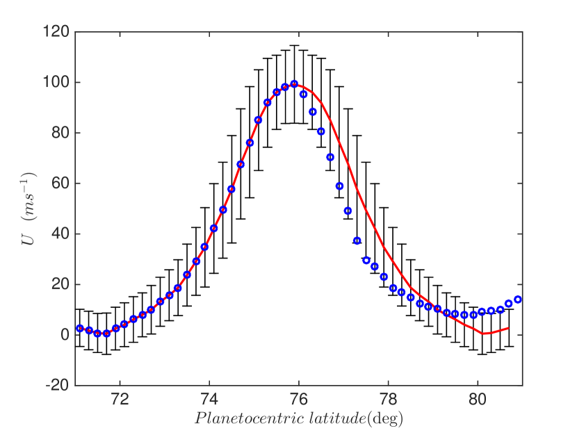
Figure 1: Observed NPJ velocity (circles) from Ref. (Antuñano et al., 2015). The observed jet has been symmetrized by reflecting its southern flank about the jet maximum (solid line with one standard deviation error bounds).

The S3T dynamics for the evolution of the first two cumulants of the flow takes the form:

$$\frac{\textrm{d}U}{\textrm{d}t} =\sum_{k}~{}\langle\overline{v^{\prime}q^{\prime}}_{\psi}\rangle_{k}-r_{m}U~{},$$ (18a)

$$\frac{\textrm{d}H}{\textrm{d}t} =D^{-2}_{\lambda}D^{2}\sum_{k}\langle\overline{v^{\prime}q^{\prime}}_{\theta}\rangle_{k}-r_{m}H~{},$$ (18b)

$$\frac{\textrm{d}\bm{\mathsf{C}}_{k}}{\textrm{d}t} =~{}\bm{\mathsf{A}}_{k}({\cal U})\,\bm{\mathsf{C}}_{k}~{}+\bm{\mathsf{C}}_{k}\,\bm{\mathsf{A}}_{k}^{\dagger}({\cal U})~{}+~{}\varepsilon\bm{\mathsf{Q}}_{k}~{},$$ (18c)

with the vorticity fluxes given in terms of the $\bm{\mathsf{C}}_{k}$ in (14) and the operators $\bm{\mathsf{A}}_{k}$ defined in (12).

The S3T system represents the second cumulant with an infinite perturbation ensemble and it is as a result autonomous and therefore has the very useful property for theoretical investigation of providing exact stationary fixed point solutions for statistical equilibrium states. Because the excitation is spatially homogeneous the zero mean flow, $U=H=0$, together with the perturbation field, $\bm{\mathsf{C}}_{k}^{e}$, satisfying the corresponding steady state Lyapunov equations, is an equilibrium solution for any $\varepsilon$ (18c) (for the explicit expression of the equilibrium covariance see Ref. DelSole and Farrell (1995)). However, this homogeneous equilibrium state is unstable in the S3T system for $\varepsilon$ greater than a critical $\varepsilon_{c}$. This critical value of excitation rate resulting in unstable jet growth in the S3T system can be found by analyzing the stability of perturbations from this equilibrium state using the perturbation form of (18) (cf. Ref. (Farrell and Ioannou, 2008)). As $\varepsilon$ is increased beyond $\varepsilon_{c}$ this instability results in a bifurcation in which finite amplitude jet equilibrium solutions, ${\cal U}^{e}=[U^{e},H^{e}]$, emerge with associated covariances $\bm{\mathsf{C}}_{k}^{e}$ that satisfy the time independent equilibrium state of  (18) for this $\varepsilon$. These equilibria are stable for a range of $\varepsilon$ and satisfy the steady state equations:

$$\sum_{k}\langle\overline{v^{\prime}q^{\prime}}_{\psi}\rangle_{k}=r_{m}U^{e}~{},~{}~{}D^{2}\sum_{k}\langle\overline{v^{\prime}q^{\prime}}_{\theta}\rangle_{k}=r_{m}D^{2}_{\lambda}H^{e}~{},$$ (19a)

$$\bm{\mathsf{A}}_{k}({\cal U}^{e})\,\bm{\mathsf{C}}_{k}^{e}+\bm{\mathsf{C}}_{k}^{e}\,\bm{\mathsf{A}}_{k}^{\dagger}({\cal U}^{e})=-\varepsilon\bm{\mathsf{Q}}_{k}~{}.$$ (19b)

Remarkably, these equilibria exist even for $r_{m}=0$. This limit is especially useful for theoretical investigation because the associated equilibria have a universal form: when $r_{m}=0$ it follows from the linearity of (19b) that if ${\cal U}^{e}$, $\bm{\mathsf{C}}_{k}^{e}$ (for the excited $k$) is an equilibrium solution for $\varepsilon=1$ then the same ${\cal U}^{e}$ is an equilibrium solution with $\varepsilon C_{k}^{e}$ for any $\varepsilon$. It does take longer to reach the equilibrium state with small $\varepsilon$ but the same equilibrium is eventually established by nonlinear feedback regulation between the mean and perturbation equations. However, it is important to note that for large enough $\varepsilon$ this equilibrium solution may itself become S3T unstable.

III Parameters

The first 56 zonal wavenumbers, $k=2\pi n/L_{x}$ with $n=1,\dots,56$, are excited in the perturbation dynamics. These are referred to alternatively as global wavenumbers or as waves $n=1,\dots,56$. The simulations use $64$ grid points in $y$ with convergence verified by doubling this resolution. The stochastic excitation has Gaussian structure in $y$ with $\bm{\mathsf{F}}_{k}$ chosen so that the $(i,j)$ element of the excitation is proportional to $e^{-(y_{i}-y_{j})^{2}/\delta^{2}}$, with $\delta=1$. Recall that the associated excitation covariances in the S3T dynamics, $\bm{\mathsf{Q}}_{k}$, are normalized so that each wavenumber provides the same energy injection rate and that with $\varepsilon=1$ the total energy injection rate over all wavenumbers is dimensionally $10^{-4}~{}\rm W\,kg^{-1}$. We have chosen for modeling the NPJ a doubly periodic channel with parameter values: $L_{y}=10^{4}~{}\rm km$, $L_{x}=8\times 10^{4}~{}\rm km$, $\beta_{sat}(74^{\circ})=1.6\times 10^{-12}~{}\rm m^{-1}\,s^{-1}$, $\lambda=10^{-3}~{}\rm km^{-1}$, perturbation damping $r_{p}=0.2~{}\rm day^{-1}$ and excitation $\varepsilon=1$.

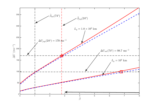
Figure 2: S3T equilibrium jet amplitude, $\Delta U$, as a function of $\tilde{\beta}=\beta/\beta_{sat}(74^{\circ})$ in the low jet damping regime. $\Delta U$ is the difference between the maximum and the minimum jet velocities. Indicated are values of $\tilde{\beta}$ for Saturn’s NPJ ($L_{y}=10^{4}~{}\rm km$) and for Jupiter’s $24^{\circ}\;\rm N$ jet ($L_{y}=1.8\times 10^{4}~{}\rm km$). The equilibria for this case in which equal excitation has been imposed in both layers are barotropic and continuous lines indicate these equilibria for $r_{m}=0$. Dashed lines showing these equilibria for $r_{m}=0.001~{}\rm day^{-1}$ differ little indicating the validity of the $r_{m}=0$ asymptotic. The dependence on $\varepsilon$ and $r_{p}$ of these asymptotic jets is also very weak and is not shown. The asymptotic scaling of the jet amplitude $\Delta U$ with $\beta L_{y}^{2}$ is nearly perfect for $\tilde{\beta}>3$ (marked with an arrow). Also indicated are the planetary values of $\tilde{\beta}_{sat}(74^{\circ})$, $\tilde{\beta}_{jup}(24^{\circ})$, the observed $\Delta U_{sat}(74^{\circ})=98.7~{}\rm m\,s^{-1}$ from Ref. (Antuñano et al., 2015) and the observed $\Delta U_{jup}(24^{\circ})=170~{}\rm m\,s^{-1}$ from Ref. Sánchez-Lavega et al. (2008). While the observed $\Delta U_{jup}(24^{\circ})$ (star) is consistent with the planetary value of $\beta$ as predicted by the asymptotic theory, the observed $\Delta U_{sat}(74^{\circ})$ (square) requires $\tilde{\beta}=6.9$ for consistency.

IV Universal structure and amplitude scaling of weakly damped turbulent jets

The velocity structure of the NPJ is asymmetric presumably because the jet is influenced by encroachment of the polar vortex flow on its north side (cf. Fig. 1). For simplicity we model a symmetric channel and consistently choose to compare our results with a symmetrized jet obtained by reflecting the southern half of the observed jet structure about the jet maximum. This symmetrized jet together with one standard deviation error bounds as tabulated in (Antuñano et al., 2015) is shown in Fig. 1.

We anticipate that the jet dynamics will be in the small jet damping regime in which the exact value of $r_{m}$ is irrelevant and can be taken to vanish. With the remaining parameter value given above we find that a barotropic jet with a single maximum in zonal velocity arises as an unstable S3T eigenmode. That the jet structure is barotropic is an important prediction of the SSD that remains valid at finite amplitude. Whether the jets of the gaseous planets are deep or shallow has implications for discriminating among mechanisms for jet formation. We conclude that the dynamics favors deep jets. A further implication is that imposition of a finite Rossby radius in a barotropic model would not be physically justified. Consistent with the barotropic structure of the jets, we have verified that the Rossby radius has little affect on the jet dynamics. We wish to study the influence on the S3T jet and perturbation covariance of the perturbation damping rate, $r_{p}$, the amplitude of the excitation, $\varepsilon$, and $\beta$. In the limit of small $r_{m}$ the time required to reach equilibrium depends on $r_{m}$ but the final equilibrium jet structure depends to a good approximation only on the channel width and $\beta$. In this regime, the equilibrium jet amplitude and structure are nearly independent of the excitation rate, $\varepsilon$, and the perturbation damping rate, $r_{p}$, while the perturbation energy is to a very good approximation proportional to their ratio $\varepsilon/r_{p}$. The jet structure obtained in the limit $r_{m}\rightarrow 0$ is close to the observed structure so we exploit the simplicity of this limit by studying the jet dynamics with zero mean jet damping, $r_{m}=0$. Departures from the $r_{m}=0$ equilibrium solution resulting from physically relevant nonzero jet damping rates are verified to be small (cf. Fig. 2).

With $r_{m}=0$ the equilibrium jet velocity varies approximately linearly with $\beta L_{y}^{2}$ as shown in Fig. 2 in which the values of $\beta$ appropriate for Saturn’s NPJ and for Jupiter’s $24^{\circ}\;\rm N$ jet are indicated. As $\beta$ increases the equilibrium jet assumes a universal structure with this $\beta L_{y}^{2}$ scaling, as shown in Fig. 3. While Jupiter’s $24^{\circ}$ N jet corresponds closely with this universal scaling (cf. Fig. 3c), Saturn’s NPJ is observed to be substantially stronger at $98.7~{}\rm m\,s^{-1}$ than the approximately $30~{}\rm m\,s^{-1}$ (cf. Fig. 2) predicted by the scaling for $\beta_{sat}(74^{\circ})=1.6\times 10^{-12}~{}\rm m^{-1}\,s^{-1}$ and the NPJ channel width of $L_{y}=10^{4}~{}\rm km$. The effective value of $\beta$ required to obtain correspondence with the scaling is $\beta_{eff}=6.9\beta_{sat}(74^{\circ})$

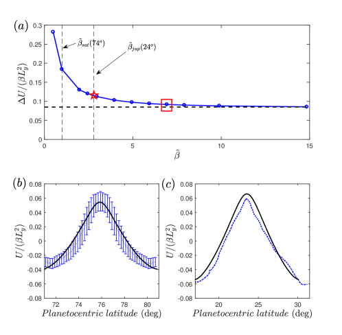
Figure 3: Universal structure of the S3T equilibrium jets for vanishing jet damping, $r_{m}=0$. Panel (a): normalized equilibrium jet amplitude, $\Delta U/(\beta L_{y}^{2})$, as a function of $\tilde{\beta}=\beta/\beta_{sat}(74^{\circ})$. For large $\tilde{\beta}$ the S3T equilibrium flows assume an asymptotic structure and amplitude $\Delta U/(\beta L_{y}^{2})\approx 0.085$. Panel (b): the observed NPJ from Ref. (Antuñano et al., 2015) which has been symmetrized, scaled and had its mean removed (dotted with error bounds) compared to the scaled S3T equilibrium jet for $\tilde{\beta}=6.9$ (indicated with a square in Panel (a)). Panel (c): the observed Jupiter $24^{\circ}\;\rm N$ jet from Ref. Sánchez-Lavega et al. (2008) with has been similarly symmetrized, scaled and had its mean removed (dotted) compared to the scaled S3T equilibrium jet for $\tilde{\beta}=2.8$ (indicated with a star in Panel (a)) for channel size $L_{y}=1.8\times 10^{4}~{}\rm km$. These barotropic equilibria are obtained with the two layers equally excited with $\varepsilon=1$ corresponding to energy injection of $10^{-4}~{}\rm W\,kg^{-1}$ and $r_{p}=0.2~{}\rm day^{-1}$. This figure confirms that these planetary jets correspond to $r_{m}=0$ S3T equilibrium solution and approach the predicted asymptotic structure as $\tilde{\beta}$ increases.

The jet equilibrium is established by a robust feedback regulation arising from interaction between the mean equation and the perturbation covariance equation. The mean jet, which is undamped, grows from an arbitrarily small perturbation in the mean flow at first exponentially under the influence of the upgradient fluxes induced by shear straining of the short waves. This growth is progressively opposed and eventually terminated by downgradient fluxes associated with the arising of this nearly neutral mode as the jet vorticity gradient sign change begins to be established (cf. Fig. 4). Extensive experience with simulations has convinced us that this incipient instability closely constrains the jet amplitude to allow only relatively small vorticity gradient sign changes to occur. It is widely recognized that the large vorticity gradient sign change in the NPJ observations poses a conundrum Antuñano et al. (2015). Within our model framework this discrepancy between the observed large vorticity gradient sign change in the observations of the upper layer of the NPJ can only be resolved by regarding the observed jet equilibrium as an indirect observation of a larger effective value of $\beta$ in the unobserved lower layer of the NPJ and in fact the S3T equilibrium jet with an appropriate choice of $\beta$, which is $\beta_{eff}=6.9\beta_{sat}(74^{\circ})$, is in close agreement with the observed NPJ jet (cf. Fig. 3b). We wish now to establish the dynamical argument compelling this conclusion.

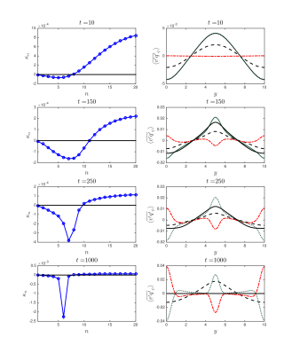
Figure 4: Left panels: normalized rate of energy input to the jet by each wave $n$, $\kappa_{n}=\int_{0}^{L_{y}}U\langle\overline{v^{\prime}q^{\prime}}_{\psi}\rangle_{n}\;\textrm{d}y\big{/}\int_{0}^{L_{y}}\tfrac{1}{2}U^{2}\;\textrm{d}y$ ($\rm day^{-1}$), for times $t=10,~{}150,~{}250,~{}1000$ as the S3T equilibrium is established starting from a small random initial jet structure. Right panels: the latitudinal distribution of the vorticity flux $\langle\overline{v^{\prime}q^{\prime}}_{\psi}\rangle$ (solid) (units: $11.57~{}\rm m\,s^{-1}\,day^{-1}$), the vorticity flux $\langle\overline{v^{\prime}q^{\prime}}_{\psi}\rangle_{>}=\sum_{n=12}^{56}\langle\overline{v^{\prime}q^{\prime}}_{\psi}\rangle_{n}$ from zonal waves $n\geq 12$ (dashed line), and the vorticity flux $\langle\overline{v^{\prime}q^{\prime}}_{\psi}\rangle_{<}=\sum_{n=1}^{11}\langle\overline{v^{\prime}q^{\prime}_{\psi}}\rangle_{n}$ from zonal waves $n<12$ (dotted line). The structure of the zonal velocity at the corresponding time is indicated with a dashed line (amplitude arbitrary chosen to fit the graph). Vorticity fluxes $\langle\overline{v^{\prime}q^{\prime}_{\psi}}\rangle_{>}$ are upgradient and are responsible for forming and maintaining the jet, vorticity fluxes $\langle\overline{v^{\prime}q^{\prime}_{\psi}}\rangle_{<}$ are downgradient opposing the jet and these are responsible for the jet equilibration. The S3T equilibrium is attained by $t=1000$ so that consistently $\langle\overline{v^{\prime}q^{\prime}}_{\psi}\rangle(y)=0$. Energy loss from the jet at equilibrium is concentrated at $n=6$ and this energy loss is primarily balanced by energy input due to waves with $n\geq 8$. Parameters: $L_{y}=10^{4}~{}\rm km$, $L_{x}=8\times 10^{4}~{}\rm km$, $\varepsilon=1$ corresponding to equal energy injection in both layers of $10^{-4}~{}\rm W\,kg^{-1}$, $r_{m}=0$ , $r_{p}=0.2~{}\rm day^{-1}$ and $\tilde{\beta}=6.9$.

V The equilibration mechanism underlying the robust scaling of weakly damped turbulent jets

We turn now to study in more detail the mechanism underlying the universal scaling of the structure and amplitude of weakly damped turbulent jets.

Note that in an undamped jet at equilibrium the perturbation momentum flux divergence vanishes at each latitude, $\overline{v^{\prime}q^{\prime}}(y)=0$ (cf. $t=1000$ right panel of Fig. 4). Moreover, this requirement is independent of the stochastic excitation amplitude, $\varepsilon$. As previously mentioned, for a given $\varepsilon$, perhaps from observational constraints, the energy of the perturbation field at equilibrium can be shown to increase inversely with perturbation damping, $r_{p}$, to a good approximation. These considerations imply invariant structure at equilibrium in the small $r_{m}$ limit for both the jet (cf. Fig. 3) and the perturbation turbulence component with only the amplitude of the perturbation turbulence component varying and that variation being as the ratio of excitation to damping, $\varepsilon/r_{p}$.

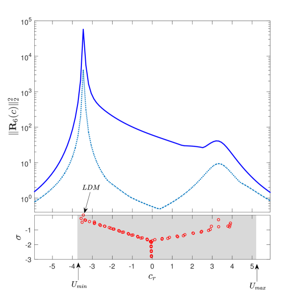
Figure 5: Top panel: the square of the energy norm of the resolvent for $n=6$, $\|{\bf R}_{6}(c)\|_{2}^{2}$, (solid) as a function of phase speed, $c$, indicating the maximum energy amplification over all latitudinal structures $f(y)$ for unit energy harmonic forcing of the form $f(y)\,e^{{\rm i}k(x-ct)}$ with $k=2\pi n/L_{x}$. Also shown is the square of the energy norm of the equivalent normal resolvent which would obtain if the eigenfunctions of $\bm{\mathsf{A}}_{k}$ were orthogonal (dotted). In the bottom panel is shown the growth rate, $\sigma$, and phase speed, $c_{r}$, of the modes of $\bm{\mathsf{A}}_{k}$ for $n=6$ (circles). The dominant response arises in association with the nearly neutral least damped mode (indicated LDM) with $c=-3.44$ and critical layer inside the retrograde jet. Although the secondary peak in the prograde jet associated with the mode with phase speed $c=3.32$ arises in association with a prominent sign change in vorticity gradient the associated modes are not significant in giving rise to the fluxes responsible for equilibrating the jet. The equivalent normal response is substantially smaller than the actual response indicating that non-normal interactions dominate the energetics at all phase speeds and most importantly at the phase speed of the LDM where the maximum interaction occurs. Quantities are non-dimensional and parameters as in Fig. 4.

In addition to its anomalously large amplitude given the small planetary value of $\beta$ available to stabilize it, the NPJ is also remarkable for supporting a prominent wavenumber six perturbation with the amplitude required to distort the jet into a distinct hexagonal shape. S3T equilibria comprise both the structure of the mean jet and the perturbation covariance from which information on perturbation structure can be determined. A temporal sequence showing establishment of the equilibrium structure of the NPJ starting from a random initial condition and assuming the inferred $\tilde{\beta}=6.9$ is shown in Fig. 4. As is generally found, the upgradient fluxes are produced by the short waves (Kitamura and Ishioka, 2007; Farrell and Ioannou, 2009b), which in the case of the NPJ means waves with $n>12$. The transfer of perturbation energy of wave $n$ to the mean is quantified by $\kappa_{n}=\int_{0}^{L_{y}}U\langle\overline{v^{\prime}q^{\prime}}_{\psi}\rangle_{n}\;\textrm{d}y\big{/}\int_{0}^{L_{y}}\tfrac{1}{2}U^{2}\;\textrm{d}y$ ($\rm day^{-1}$) and plotted in Fig. 4. Conversely, downgradient fluxes are produced by the long waves with $n\leq 8$. The upgradient fluxes are associated with shear straining of the short waves which can be regarded as a mechanism resulting in a negative viscosity in that it produces upgradient momentum flux proportional to the velocity gradient (Bakas and Ioannou, 2013a) as is observed in the atmospheres of both Jupiter and Saturn (Ingersoll et al., 2004; Salyk et al., 2006; Delgenio et al., 2007). This shear straining mechanism accelerates both the prograde and retrograde jets. When the homogeneous turbulence is perturbed by a random mean jet these upgradient fluxes immediately cause the jet to grow in the form of the most unstable S3T eigenmode (cf. time $t=10$ in Fig. 4) (Farrell and Ioannou, 2007, 2008). As the jet amplitude increases the retrograde jet progressively exceeds the speed of the slower retrograde Rossby modes and these sequentially obtain critical layers inside the retrograde jet (Kasahara, 1980). Approach to and attainment of a critical layer by these modes is accompanied by increasing modal as well as non-normal energetic interaction with the jet resulting in increasing downgradient fluxes opposing the growth of the S3T jet eigenmode so as to eventually establish a nonlinear equilibrium. As neutral stability is approached with increasing jet amplitude these fluxes come into balance establishing by time $t=1000$ the stable fixed point equilibrium turbulent jet structure and associated perturbation covariance that together constitute a complete solution for the turbulent state at second order as shown in Fig. 4. The equilibrium shown in Fig. 4 reveals the mechanisms responsible for forcing the large scale jet and also the mechanism of dissipation at large scales that equilibrates the jet: the jet receives energy from the small scale incoherent components of the turbulence, rises to finite amplitude and equilibrates by transferring energy to the wave six structure, which provides the sink for the jet energy. Note that in this planetary scale turbulence regime both the upscale energy transfer forcing the jet and the downscale energy transfer to the wave six mode regulating its amplitude are nonlocal in spectral space and neither involves a turbulent cascade.

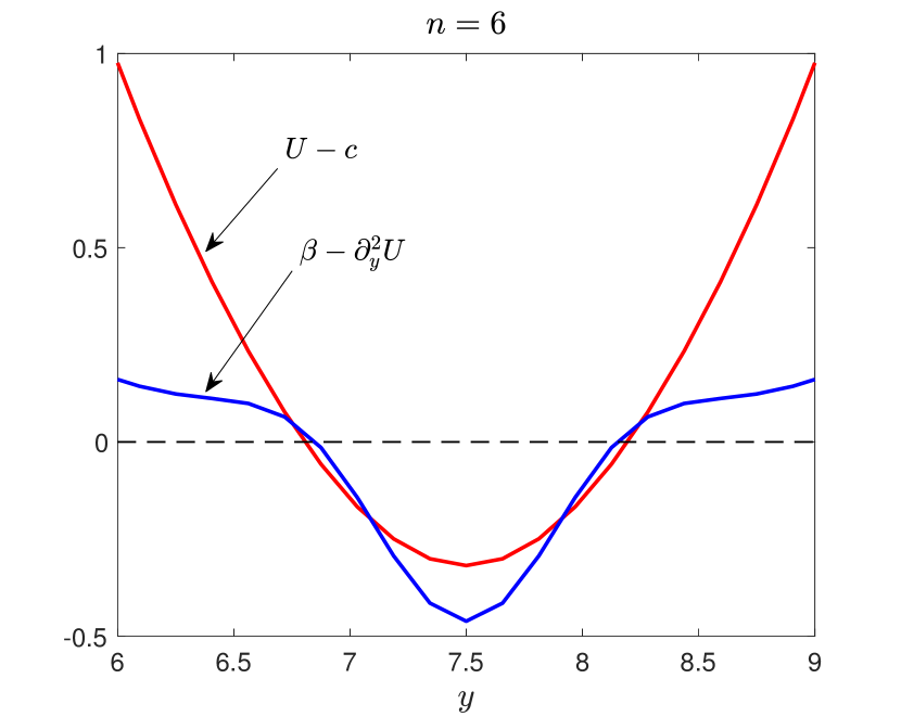
Figure 6: Detail near the minimum velocity of the retrograde S3T jet at equilibrium with $\tilde{\beta}=6.9$ showing the critical layer of the LDM, $U(y)-c_{r}$, where $c_{r}$ is the phase speed of the nearly neutral LDM of $\bm{\mathsf{A}}_{k}$ for $n=6$. Also shown is the jet vorticity gradient, $\beta-\partial_{y}^{2}U$, as a function of $y$. Note that the perturbation-mean interaction has stabilized the LDM by nearly eliminating the vorticity gradient in the vicinity of this mode’s critical layer while leaving a small change in vorticity gradient sign between the mode’s critical layers. Such changes in sign of the vorticity gradient are a commonly observed feature of turbulent jets in planetary atmospheres. Quantities are non-dimensional and parameters as in Fig. 4.

Further insight into the dynamics can be obtained by calculating the eigenvalues and the resolvent of the perturbation dynamics operator $\bm{\mathsf{A}}_{k}({\mathbf{U}})$ as the jet structure $\mathbf{U}$ evolves toward equilibrium. The eigenvalues reveal the approach of the retrograde modes’ phase speeds to the speed of the retrograde jet and the associated decrease in mode damping rate which is indicative of energetic interaction with the jet and diagnostic of downgradient momentum flux by the mode. The resolvent of $\bm{\mathsf{A}}_{k}({\mathbf{U}})$ provides more information by revealing the response of the dynamics to the turbulent excitation at each mode phase speed, $c$. We use the energy norm to measure the response of the dynamics and the non-normality of the dynamics are defined with respect the energy norm (cf. Ref. Farrell and Ioannou (1996)). The resolvent of perturbations with zonal wavenumber $k=2\pi n/L_{x}$ perturbations is :

$${\bf R}_{n}(c)=-({\rm i}kc~{}\bm{\mathsf{I}}+\bm{\mathsf{A}}_{k})^{-1}~{}.$$ (20)

The square norm of the resolvent of $\bm{\mathsf{A}}_{k}({\mathbf{U}})$, which is the energy spectrum as a function of phase speed for temporally and spatially delta correlated excitation, is shown together with the spectrum of the modes of $\bm{\mathsf{A}}_{k}({\mathbf{U}})$ for the equilibrium jet structure, $\mathbf{U}$, in Fig. 5. There is a dominant nearly neutral Rossby mode with wavenumber six that is responsible for most of the downgradient momentum flux balancing the upgradient shear straining fluxes from the short waves (cf. Fig. 4 at $t=1000$). This wave dominates the response of the dynamics to perturbation when the jet is equilibrated as can be inferred from the resolvent. This dominance of wavenumber six in the perturbation variance extends over a wide range in $\beta$ and therefore in equilibrium jet amplitude as shown in Fig. 2. Note that the phase speed of this mode has been incorporated into the retrograde jet but that this mode remains stable consistent with finiteness of the perturbation variance. The strong $\overline{v^{\prime}q^{\prime}}$ fluxes associated with the maintenance of this mode have forced the gradient of the mean vorticity in the vicinity of its critical layer nearly to zero as shown in Fig. 6. This nonlinear interaction provides an example of the mechanisms at play in the complex feedback stabilization process operating between the first and second cumulants in the S3T dynamics that results in establishment of the equilibrium statistical state. It is useful to regard this interaction as a nonlinear regulator that continuously adjusts the mean flow to a state that is in neutral equilibrium with the perturbation dynamics by enforcing vanishing of the mean vorticity gradient at the critical layers of the dominant perturbation modes in the retrograde jet. This consideration explains why strongly excited jet equilibria in planetary atmospheres commonly exhibit easily observable changes in sign of the mean vorticity gradient without incurring instability: shear straining of the small turbulence components drives both the prograde and retrograde jets strongly producing the sign change while the regulator need only equilibrate any incipient modal instability by enforcing vanishing of the gradient at the mode critical layer while leaving a substantial vorticity sign change between the critical layers in the jet profile. It is important to appreciate the crucial role of active feedback regulation continually operating between the first and second cumulants in the SSD in maintaining the stability of this turbulent equilibrium jet-wave-turbulence state. If one were simply to postulate a jet profile very much like the observed it would be extremely unlikely to have by chance the vanishing gradient of vorticity precisely at the critical layers of the mode required for stability of the jet structure. Viewed another way, the existence of strong jet equilibria with the structure seen in planetary atmospheres requires that an active feedback regulation be operating to maintain their stability. Note that the mechanism of vorticity mixing in the retrograde jets could not result in a negative vorticity maximum as is seen in both observations and our simulations.

While it is tempting to regard the downgradient momentum fluxes arising from the dominant mode itself as being primarily responsible for opposing the upgradient fluxes by the small waves, the resolvent tells a different story. Shown in Fig. 5 is both the response of the jet dynamics to perturbation as a function of phase speed and the response that would be produced by the modes assuming they were independent; that is, assuming the modes to be orthogonal in energy. This so called equivalent normal response reveals that the energetics and therefore the fluxes associated with the LDM at $n=6$ are being produced by non-normal interaction among the modes rather than by the $n=6$ mode by itself. In fact it is generally the case in systems non-normal in energy that transient growth of the adjoint of a mode is responsible for establishing a mode’s equilibrium amplitude when it is excited stochastically rather than growth of the mode itself (Farrell and Ioannou, 1996).

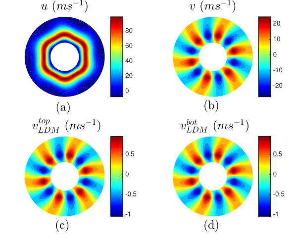
Figure 7: The predicted NPJ velocity structure in a polar rendering of the S3T model channel (the external circle of the annulus corresponds to latitude $70^{o}$ and the inner circle to $82^{o}$). Panel (a): contours of the total zonal velocity obtained by adding the S3T equilibrium zonal mean velocity and the zonal velocity of the first POD mode obtained from eigenanalysis of the equilibrium perturbation covariance at zonal wavenumber $n=6$. This mode accounts for $99.5\%$ of the perturbation energy at this wavenumber. The amplitude of the wave is obtained from the associated eigenvalue of the equilibrium perturbation covariance. The jet is barotropic as is the $n=6$ wave. Panel (b): contours of the meridional velocity of the first POD of the perturbation covariance at zonal wavenumber $n=6$. Panels (c) and (d) show respectively the structure in the top and bottom layer of the least damped mode (LDM) of $\bm{\mathsf{A}}_{k}$ at $n=6$ (cf. Fig. 5). It is clear from this comparison that the LDM is barotropic and the POD has the structure of this mode. Parameters are as in Fig. 4.

Figure 8: Top panel: S3T equilibrium jet amplitude, $\Delta U$, as a function of the normalized barotropic $\beta$ component $\tilde{\beta}_{\psi}=\beta_{\psi}/\beta_{sat}(74^{\circ})$ for Saturn’s NPJ ($L_{y}=10^{4}~{}\rm km$). $\Delta U_{1}$ is the difference between the maximum and the minimum jet velocities of the top layer. Lines $E_{1,2}$ indicate equilibria obtained when both layers are equally excited, lines $E_{1}$ indicate equilibria obtained when only the top layer is excited. The solid and dashed lines are equilibria with bottom layer $\beta_{2}=2\beta_{\psi}-\beta_{sat}$ and top layer $\beta_{1}=\beta_{sat}$. The dash-dot and dotted lines indicate equilibria in which both layers have the same $\beta_{\psi}$, as in Fig. 2. Also indicated are the planetary values of $\tilde{\beta}_{sat}(74^{\circ})$ and the observed $\Delta U_{sat}(74^{\circ})=98.7~{}\rm m\,s^{-1}$ from Ref. (Antuñano et al., 2015); boxes indicate the point consistent with the NPJ observations . The arrow indicates the range of $\beta_{\psi}$ for which the perturbation energy is concentrated in a single nearly neutral wave with phase speed near that of the jet minimum, which for the NPJ channel corresponds to $n=6$. Scaling of $\Delta U$ with $\beta L_{y}^{2}$ is highly accurate in this region. Parameters: $r_{m}=0$, $\varepsilon=1~{}\rm W\,kg^{-1}$, $L_{R}=10^{3}~{}\rm km$, $r_{p}=0.2~{}\rm day^{-1}$. Bottom panel: The resulting baroclinicity of the equilibria, measured as the ratio of $\Delta U_{2}/\Delta U_{1}$ in each layer. Barotropic flows, such as occur when the excitation and $\beta$ are the same in both layers (cases $E_{1,2}$) have $\Delta U_{2}/\Delta U_{1}=1$ (dash-dot line). In all other cases the equilibria are slightly baroclinic. When the upper layer alone is excited ($E_{1}$) the upper layer jet is stronger than the jet in the bottom layer (solid and dotted lines). If both layers are excited and the value of $\beta$ in the bottom layer is greater than that in the top layer, the bottom jet is the stronger (dashed line).

Because of its dominance the structure of the $n=6$ perturbation can be obtained as the first eigenmode of the perturbation covariance (referred to variously as the leading proper orthogonal decomposition (POD) or empirical orthogonal function (EOF) mode). This structure is shown in Fig. 7b and its superposition on the jet with amplitude obtained as the RMS of its variance as obtained from the associated POD eigenmode is shown in Fig. 7a. Consistent with the resolvent diagnostic discussed above, this mode has nearly the same barotropic structure as the least damped mode of the linear perturbation dynamics, shown in Fig. 7c,d. The prediction of the theory that the wave six phase speed be just inside the retrograde jet is in agreement with observations (Antuñano et al., 2015).

The amplitude of the wave six mode is proportional to $\varepsilon/r_{p}$ and we have chosen physically plaussible values for these unknown parameters, $\varepsilon=1$ and $r_{p}=0.2~{}\rm day^{-1}$, corresponding to excitation of $10^{-4}~{}\rm W\,kg^{-1}$. However, other combinations of $\varepsilon$ and $r_{p}$ with $\varepsilon/r_{p}=5$ lead to equilibria very close to those obtained with these parameter values.

VI The deep stable layer NPJ model

Our study of the dynamical consequences for jet formation and equilibration of varying the planetary value of $\beta$ reported above has the advantage of allowing the underlying mechanisms and the associated scaling to be understood in a simple context. However, the physical mechanism by which an effective value of $\beta$ differing from the planetary value enters the dynamics of the NPJ is likely to be a poleward sloping surface of concentrated downward increase in static stability underlying the deep jet inducing the dynamic analogue of a topographic $\beta$ effect in the lower layer. This equivalent sloping lower boundary could be associated with constitutive, convective and/or dynamical processes analogous to those which are responsible for maintaining the Earth’s tropopause but lacking observation it is not possible to identify the specific processes responsible.

A topographic $\beta$ effect results in different values of effective $\beta$ in the two layers rather than the same value in both as was appropriate when varying the planetary value of $\beta$ in the theoretical development above. In the top layer the zonal mean potential vorticity gradient (PV gradient) is $Q_{1y}=\beta_{sat}-\partial_{y}^{2}U_{1}+\lambda^{2}(U_{1}-U_{2})$, with $\beta_{sat}$ designated the planetary value of $\beta$, and in the bottom layer it is $Q_{2y}=\beta_{sat}+\beta_{h}-\partial_{y}^{2}U_{2}-\lambda^{2}(U_{1}-U_{2})$, in which the planetary value of $\beta$ has been designated $\beta_{sat}$ and the topographic value $\beta_{h}$. The equations (1) are modified as follows:

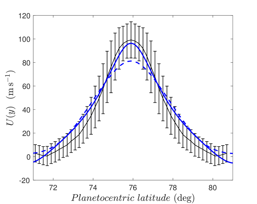
Figure 9: For the deep stable layer NPJ model: equilibrium jet in the top layer (thick solid line) and bottom layer (thick dashed line). Also shown is the symmetrized observed NPJ from Ref. (Antuñano et al., 2015) (thin dashed line with one standard deviation error bounds). The S3T equilibria are obtained with stochastic forcing of the top layer, $r_{m}=0$, $\lambda=1$ and $\tilde{\beta}_{\psi}=4.9$ corresponding to topographic component $\tilde{\beta}_{h}=8.8$ in the bottom layer. This equilibrium profile is insensitive to variations in $\varepsilon$, $r_{p}$ and $\lambda$.

$$\partial_{t}\Delta\psi+ J(\psi,\Delta\psi)+J(\theta,\Delta\theta)$$

$$+\partial_{x}\beta_{\psi}\psi+\beta_{\theta}\partial_{x}\theta=-r\Delta\psi+\sqrt{\varepsilon}\,f_{\psi}~{},$$ (21a)

$$\partial_{t}\Delta_{\lambda}\theta+ J(\psi,\Delta_{\lambda}\theta)+J(\theta,\Delta\psi)$$

$$+\beta_{\psi}\partial_{x}\theta+\beta_{\theta}\partial_{x}\psi=-r\Delta_{\lambda}\theta+\sqrt{\varepsilon}\,f_{\theta}~{},$$ (21b)

with the barotropic, $\beta_{\psi}$, and baroclinic, $\beta_{\theta}$, defined as:

$$\beta_{\psi}\stackrel{{\scriptstyle\mathrm{def}}}{{=}}\beta_{sat}+\beta_{h}/2~{},~{}~{}\beta_{\theta}\stackrel{{\scriptstyle\mathrm{def}}}{{=}}\beta_{sat}-\beta_{h}/2~{}.$$ (22)

The S3T system is modified accordingly. From  (21) we see that the effective value of $\beta$ seen by waves with primarily barotropic structure such as the planetary wave $n=6$ that is implicated in the dynamics of the NPJ equilibration is the sum of the planetary value $\beta_{sat}$ and half the topographic value, $\beta_{h}$. Results similar to those shown in Fig. 2 for the case of equal $\beta$ in both layers are shown in Fig. 8 for the case of a topographic $\beta$ effect with $\beta=\beta_{sat}+\beta_{h}$ in the bottom layer and $\beta=\beta_{sat}$ in the top layer. Even with equal excitation of the background turbulence in both layers ($E_{12}$ case) both the jet and the waves become slightly baroclinic as seen in Fig. 8 and the jet in this case obtains a higher equilibrium amplitude in the lower layer consistent with the higher effective value of $\beta$ there. However, when excitation is restricted to the top layer ($E_{1}$ case in Fig. 8) the jet in the top layer is the stronger.

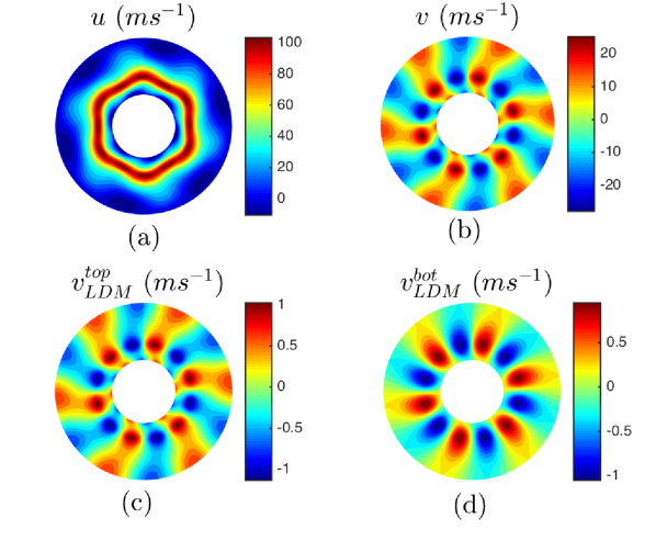
Figure 10: For the deep stable layer NPJ model shown in Fig. 9: NPJ structure in a polar rendering of the channel (the external circle of the annulus corresponds to latitude $70^{o}$ and the inner circle to $82^{o}$). Panel (a): contours of the total zonal velocity as obtained by adding to the S3T equilibrium zonal mean velocity the zonal velocity of the first POD of the equilibrium perturbation covariance at zonal wavenumber $n=6$ which accounts for $99.7\%$ of the perturbation energy at this wavenumber. The amplitude of the wave is obtained from the associated eigenvalue of the equilibrium covariance. The jet and the $n=6$ wave are slightly baroclinic. Panel (b): contours of the meridional velocity of the first POD of the perturbation covariance at zonal wavenumber $n=6$. Panels (c) and (d) show respectively the structure of the least damped mode (LDM) of $\bm{\mathsf{A}}_{k}$ for $n=6$ (indicated in Fig. 11) in the top and bottom layer (left and right panels respectively). The POD has the structure of this mode and both are slightly baroclinic. For $\varepsilon=0.7$, other parameters as in Fig. 9.

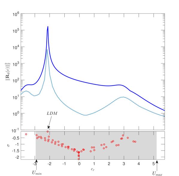
Figure 11: For the deep sloping stable layer NPJ model equilibrium shown in Fig. 9: in the top panel is shown the square of the energy norm of the resolvent for wave $n=6$, $\|{\bf R}_{6}(c)\|_{2}^{2}$ (solid), together with the equivalent normal response (dotted) as a function of phase speed, $c$. The dominant response arises from the nearly neutral least damped mode (indicated LDM) with $c=-2.14$ and critical layer inside the retrograde jet. Note the secondary peak caused by the non-normal excitation of the mode with $c=2.93$ and critical layer inside the prograde jet (see Fig. 14). In the bottom panel is shown the growth rate, $\sigma$, and phase speed, $c$, of the modes of $\bm{\mathsf{A}}_{k}$ for $n=6$ (circles). The equivalent normal response is substantially smaller than the actual response indicating that non-normal interactions dominate the energetics at all phase speeds and most importantly at the phase speed of the LDM where the maximum interaction occurs. Quantities are non-dimensional and parameters as in Fig. 9.

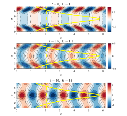
Figure 12: For the deep sloping stable layer NPJ model equilibrium shown in Fig. 9: establishment of the $n=6$ LDM by its optimal excitation in energy structure. Shown is the evolution of the optimal as indicated in the top layer streamfunction. Upper panel: the optimal perturbation at $t=0$ with energy density $E=1$. Middle panel: the evolved optimal at $t=0.5$. Bottom panel: the evolved optimal at $t=10$ at which time it has assumed the structure of the LDM with energy $E=14$. Contours indicate non-dimensional values of the streamfunction. Also shown is the equilibrium jet (solid), which has been scaled to fit, and the phase speed of the LDM (dashed). While the amplitude of the LDM is concentrated in the prograde jet, its optimal excitation is concentrated near its critical layer in the retrograde jet. The non-normality of the dynamics is indicated by both the large excitation of this stable structure and the substantial structural change during the evolution of the optimal.

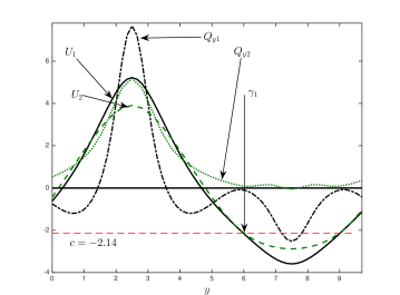
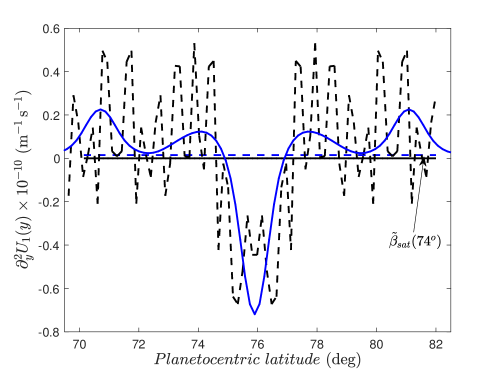
Figure 13: For the deep sloping stable layer NPJ S3T equilibrium shown in Fig. 9: top layer velocity, $U_{1}$ (solid), bottom layer velocity, $U_{2}$ (dashed), corresponding top layer PV gradient, $Q_{y1}$ (dash dot) and bottom layer PV gradient, $Q_{y2}$ (dot). Also indicated is the phase velocity of the LDM with wavenumber $n=6$ that is the dominant perturbation in producing downgradient fluxes. Note that this LDM has eliminated the PV gradients in the vicinity of its critical layers in the top and bottom layers indicated by $\gamma_{1}$. Elimination of the PV gradient at the critical layer is responsible for suppressing instability of this LDM. The strong reversal in $Q_{y1}$ at the center of the retrograde jet resulting from the upgradient vorticity fluxes produced by the $n>8$ waves remains as this region of PV gradient reversal is not opposed by the LDM which has been stabilized by elimination of the PV gradient at its critical layers. Such reversals are commonly observed in planetary atmospheres.

Figure 14: The dimensional curvature of the predicted NPJ velocity structure of the top layer jet of the S3T equilibrium shown in Fig. 9 (solid) plotted against the curvature obtained from the raw data of Ref. (Antuñano et al., 2015) (dashed line). Also indicated is the relatively insignificant planetary $\beta_{sat}(74^{\circ})$. Although noisy the data suggests both the curvature reversal in the vicinity of the prograde jet, which the theory predicts to be related to the subdominant prograde mode with non-dimensional $c=2.93$ that is responsible for the secondary maximum in the resolvent response in Fig. 11, and also the dynamically significant second maximum of the curvature in the retrograde section of the jet (at $71^{o}$ N) predicted by the theory to lie between the critical layers of the dominant $n=6$ wave with non-dimensional phase speed c= -2.14.

Assuming only the top layer is excited a topographic $\beta$ component in the lower layer of $\beta_{h}=8.8\beta_{sat}=1.44\times 10^{-11}~{}\rm m^{-1}\,s^{-1}$ when combined with the planetary $\beta_{sat}(74^{\circ})$ results in consistency with the NPJ upper layer observations as indicated in Fig. 8. With a layer depth equal to one scale height on Saturn, $H=42.1~{}\rm km$, the required lower layer slope is

$${h_{y}} = \frac{\beta_{h}H}{f}=\frac{(14.4\times 10^{-12}~{}\rm m^{-1}s^{-1})\times(42.1\times 10^{3}~{}\rm m)}{3.1\times 10^{-4}~{}\rm s^{-1}}$$

$$= 2\times 10^{-3}~{},$$

implying a density surface dynamically equivalent to the bottom boundary sloping downward toward the pole over the channel width of $10\,000~{}\rm km$ from $74.5~{}\rm km$ to $93.9~{}\rm km$ (measured from the top boundary). We remark that the prominent $24^{\circ}\;\rm N$ jet of Jupiter conforms with the lightly damped jet scaling using the planetary value of $\beta_{jup}(24^{\circ})$, as shown in Fig. 3 which result verifies previous findings (Farrell and Ioannou, 2008). This suggests that the stable lower layer inferred to underly Saturn’s NPJ is peculiar to the anomalous thermal and dynamical conditions observed near Saturn’s Pole.

The S3T jet structure in the upper layer with the parameter values given above, which were chosen to model the NPJ, is shown in Fig. 9. A polar representation of the jet and the associated $n=6$ wave is shown in Fig. 10. The jet equilibration process is essentially similar to that described in the previous section in which the planetary value of $\beta$ was varied. As in the previous case, most of the perturbation variance is concentrated in the nearly neutral wave six which has a critical layer inside the retrograde jet as can be seen in the resolvent response of the $n=6$ wave shown in Fig. 11. Again, this nearly neutral wave with critical layer inside the retrograde jet and with primarily non-normal energetics is in large part responsible for producing the upgradient flux to exactly cancel the downgradient flux produced by the waves $n\geq 8$ resulting in establishment of the turbulent equilibrium. In Fig. 12 is shown three snapshots of the temporal development of the optimal initial condition for exciting the LDM demonstrating the dominance of non-normal dynamics in the establishment of this mode. It is interesting to note that the optimal excitation of this mode, which is its adjoint (Farrell, 1988; Farrell and Ioannou, 1996), is initially concentrated in the retrograde jet (cf. Fig. 12). As in the previous example and as is required for neutrality, the PV gradient in both the upper and lower critical layers ($Q_{y1}$ and $Q_{y2}$) is eliminated, primarily by fluxes arising from the non-normal dynamics, as shown in Fig. 14.

The potential vorticity gradient reversals seen in Fig. 14, which are observed in both Jupiter and Saturn and predicted by the S3T equilibria, provide a probe of the dynamical processes at work in the equilibration of these large amplitude jets. As previously discussed in connection with the planetary $\beta$ variation example, a strong reversal of $Q_{y1}$ near the minimum of the retrograde jet results from upgradient vorticity fluxes produced by the $n>8$ waves. The resulting region of potential vorticity gradient reversal is not opposed by the LDM which enforces its own stabilization by eliminating the PV gradient in the vicinity of its critical layers leaving an extensive region between these critical layers in which the potential vorticity gradient is negative, making the flow over the whole domain violate the Rayleigh–Kuo necessary condition for instability (the relevant criterion for the two-layer model is the Charney-Stern criterion, but this reduces to the Rayleigh–Kuo criterion for nearly barotropic flows). It should be noted that violation of the Rayleigh–Kuo criterion does not guarantee the instability of the flow and so on a logical level the violation of the Rayleigh–Kuo criterion observed in most jets on Jupiter and Saturn does not present a conundrum, except for the fact that in almost every case in which the Rayleigh–Kuo condition is violated the flow is found to be unstable. It is demonstrated in this paper that the process of adjustment to statistical equilibrium actively modifies the equilibrium jets that violate the Rayleigh–Kuo condition to neutrality by placing the critical layer of the incipient unstable wave in coincidence with the location at which the mean potential vorticity vanishes, in this way equilibrating the instability.

Note that the bottom layer PV gradient has also been eliminted in the region between the critical layers of the $n=6$ wave. However, in this case with excitation limited to the top layer the shorter waves do not penetrate adequately into the bottom layer to produce sufficiently strong upgradient fluxes to form a PV gradient reversal.

Reversals in PV gradient in the retrograde jet are associated with positive curvature of the mean flow. The predicted curvature of the mean flow in the top layer is plotted in Fig. 14 against raw observations from Ref. (Antuñano et al., 2015). Discussion tends to center on the maximum at the wings of the prograde jet which is responsible for supporting modes associated with the secondary maximum in the resolvent at phase speeds inside the prograde jet seen in Fig. 11. However, the modes associated with this prograde jet PV reversal are insignificant in the dynamics. The dynamically significant PV gradient reversal is that between the critical layers of the dominant $n=6$ wave. Neither of these features is well resolved in the data but we believe that better observations of the PV in the retrograde jets would resolve the dynamically significant reversal between the $n=6$ critical layers.

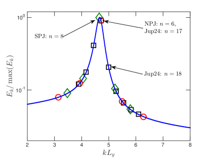
Figure 15: Normalized energy spectrum, $E_{k}/\max(E_{k})$, supported by perturbations to a finite $\beta$ approximation of the universal jet as a function of zonal wavenumber $kL_{y}$, where $L_{y}$ is the width of the approximate universal jet. $E_{k}$ is the perturbation energy maintained at $k$ when the universal velocity profile, shown in Fig. 3, is stochastically excited with equal energy injection rate at each wavenumber. The perturbation energy spectrum has a strong peak at $kL_{y}=4.66$. Waves $n=4,\dots,8$ in Saturn’s northern polar jet (with $L_{y}=10^{3}~{}\rm km$ and $k=2\pi n/L_{x}$ with $L_{x}=80\times 10^{3}~{}\rm km$) are indicated with circles. Waves $n=6,\dots,10$ in Saturn’s southern polar jet (with $L_{y}=1.2\times 10^{3}~{}\rm km$ and $k=2\pi n/L_{x}$ with $L_{x}=130\times 10^{3}~{}\rm km$) are indicated with diamonds. Waves $n=14,\dots,22$ in Jupiter’s $24^{o}$N jet (with $L_{y}=1.8\times 10^{3}~{}\rm km$ and $k=2\pi n/L_{x}$ with $L_{x}=407\times 10^{3}~{}\rm km$) are indicated with squares.

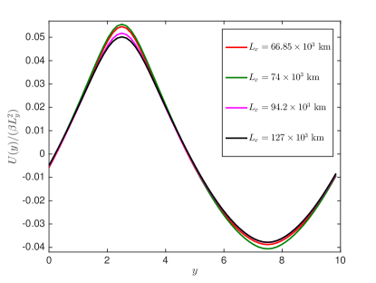
Figure 16: S3T equilibrium jets for channels with $L_{x}=66.85\times 10^{3}~{}\rm km$, $L_{x}=74\times 10^{3}~{}\rm km$, $L_{x}=94.2\times 10^{3}~{}\rm km$ and $L_{x}=127\times 10^{3}~{}\rm km$. The jets are very close to the universal profile, despite the differences in their stability and supporting perturbation structures as shown in Fig. 17 and Fig. 18. In all cases $L_{y}=10\times 10^{3}~{}\rm km$, $\tilde{\beta}=6.9$, $r_{m}=0$ and $r_{p}=0.2~{}\rm day^{-1}$.

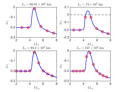
Figure 17: Maximum modal growth rate as a function zonal wavenumber $kL_{y}$ for the S3T equilibrium jets shown in Fig. 16. These jet equilibria are obtained for channels with $L_{x}=66.85\times 10^{3}~{}\rm km$, $L_{x}=74\times 10^{3}~{}\rm km$, $L_{x}=94.2\times 10^{3}~{}\rm km$, $L_{x}=127\times 10^{3}~{}\rm km$. Circles indicate the growth rates for the perturbations with zonal wavenumbers that satisfy the quantization condition in each channel. In all cases the equilibrium jet is hydrodynamically stable at these wavenumbers, but not necessarily stable at all wavenumbers, as for example in the case of $L_{x}=74$, which has been chosen so that there is no wavenumber at the peak of the resonant response where a strong instability exists. For $L_{x}=66.85\times 10^{3}~{}\rm km$ the jet maintains strongly the wave five in the channel for which $kL_{y}=4.695$ is close to the resonant peak. For $L_{x}=74\times 10^{3}~{}\rm km$ the jet maintains strongly both waves five and six for which $kL_{y}$ are respectively $4.24$ and $5.1$, which are removed further than a half-width from the resonant peak (the energy at wave 6 is half that at wave 5). For $L_{x}=94.2\times 10^{3}~{}\rm km$ the jet maintains strongly wave seven in the channel for which $kL_{y}=4.67$ is close to the resonant peak. Finally, For $L_{x}=127\times 10^{3}~{}\rm km$ the jet maintains strongly waves nine and ten (with energy at wave 10 slightly higher than the energy of wave 9) for which $kL_{y}$ are respectively $4.45$ and $4.94$. Parameters as in Fig. 16.

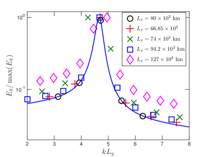
Figure 18: Comparison of the normalized energy spectrum, $E_{k}/\max(E_{k})$ supported by the equilibrium jets of Fig. 16 to the energy spectrum supported by the approximation to the universal profile. Parameters as in Fig. 16.

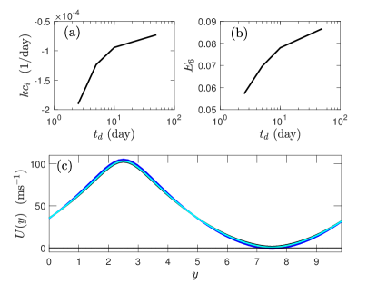
Figure 19: Dependence of the S3T equilibrium jet and associated wave six amplitude and decay rate on the dissipation rate $r_{p}$ of the small scale waves. Shown in (a) is the decay rate of the least damped mode 6 as a function the dissipation time $t_{d}=1/r_{p}\rm(day)$ imposed on waves $n>10$. Waves $n\leq 10$ are dissipated with $t_{d}=5~{}\rm day$. This figure shows that as the dissipation rate of the small scale waves with $n>10$, which are responsible for producing the upgradient fluxes forcing the jet, decreases, and the energy at these scales consistently increases, wave six approaches neutrality while its energy, shown in (b), increases. The corresponding equilibrium barotropic jet for $t_{d}=2.5,5,10,50~{}\rm day$ of the $n>10$ waves is shown in (c). This figure shows the insensitivity of the equilibrium jets to the small scale wave dissipation rate. In these simulations the energy input to each of the waves $n\leq 10$ is $1\%$ of the energy input to each of the waves with $n>10$. Other parameters $L_{x}=80\times 10^{3}~{}\rm km$, $L_{y}=10\times 10^{3}~{}\rm km$, $\tilde{\beta}=6.9$, $r_{m}=0$.

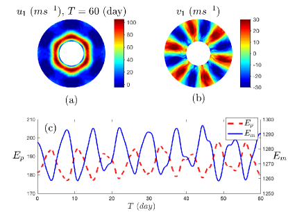
Figure 20: Snapshot of the flow in the upper layer obtained from a stochastic simulation of the QL equations with parameters that reproduce the observations. In this polar plot the external circle of the annulus corresponds to latitude $70^{o}$ and the inner circle to $82^{o}$. Shown are: contours of the total top layer zonal velocity, $u_{1}$, (a), the meridional velocity, $v_{1}$, (b), and a time series of the kinetic energy of the non-zonal component, $E_{p}$, and of the mean flow, $E_{m}$. The flow is close to barotropic. The temporal evolution of this simulation can be seen in the movie included in the Supplemental Material. The vacillation in the mean and perturbation energy, the perturbation component of which is predominantly concentrated at wave 6, reveals a compensating exchange of energy between wave 6 and the mean flow, which can be identified with the least damped S3T mode of the jet equilibrium excited by the fluctuations of the QL simulation (see Fig. 21). In these simulations the large scales waves ($n\leq 10$) are dissipated at rate $r_{p}=0.005~{}\rm day^{-1}$ while small scales waves ($n>10$) are dissipated at rate $r_{p}=0.05~{}\rm day^{-1}$. The total energy input is $1~{}\rm Wm^{-2}$ distributed equally among waves $n>10$ (the energy input to each of the waves $n\leq 10$ is $10^{-4}$ of the energy input to each of the waves with $n>10$). Other parameters $L_{x}=80\times 10^{3}~{}\rm km$, $L_{y}=10\times 10^{3}~{}\rm km$, $\tilde{\beta}=8.6$, $r_{m}=0$.

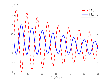
Figure 21: Oscillations resulting from perturbation to the S3T zonal jet equilibrium for the parameters in Fig. 20. Shown is the time evolution of the perturbation energy fluctuation from the equilibrium value, $\delta E_{p}$, (solid) and fluctuation of the mean energy as a departure from its equilibrium value, $\delta E_{m}$. The equilibrium covariance of the S3T jet equilibrium was perturbed with a random perturbation sufficiently small to render the dynamics of relaxation to the S3T equilibrium linear. The decaying oscillations in the energy are shown after an initial adjustment has occurred. The frequency of the oscillations matches the oscillations shown in the QL simulation in Fig. 20 and the oscillations in this figure are interpreted as revealing the least damped S3T mode about the S3T equilibrium which are being stochastically maintained by the fluctuations in the QL simulation.

VII Discussion

Statistical state dynamics at second order predicts that a stochastically excited two layer fluid in a meridionally confined channel with vanishing meridional temperature gradient and jet scale dissipation supports barotropic jets that asymptotically approach a universal structure as the channel length $L_{x}\rightarrow\infty$ and $\beta\rightarrow\infty$. The velocity of this universal jet scales as $\beta L_{y}^{2}$. Saturn’s $74^{o}$N jet, Saturn’s $70^{o}$ S jet and Jupiter’s $24^{o}$N jet closely approximate this universal structure. Associated with this barotropic mean jet is a universal equilibrium covariance satisfying the non-dimensional barotropic component of (19b):

$${\tilde{\bm{\mathsf{A}}}}_{\tilde{k}}^{\psi\psi}(\tilde{U})\,\bm{\mathsf{C}}_{\tilde{k}}^{\psi\psi}+\bm{\mathsf{C}}_{\tilde{k}}^{\psi\psi}\,{\tilde{\bm{\mathsf{A}}}}_{\tilde{k}}^{\psi\psi\dagger}(\tilde{U})=-\tilde{\varepsilon}\bm{\mathsf{Q}}_{\tilde{k}}^{\psi\psi}~{},$$ (23)

with

$$\tilde{\bm{\mathsf{A}}}_{\tilde{k}}^{\psi\psi}=\tilde{\Delta}_{\tilde{k}}^{-1}\left[-{\rm i}\tilde{k}\tilde{U}\tilde{\Delta}_{\tilde{k}}-{\rm i}{\tilde{k}}\left(1-\tilde{D}^{2}\tilde{U}\right)\right]-\tilde{r}_{p}~{},$$ (24)

in which length is scaled by $L_{y}$, time by $1/(\beta L_{y})$ and velocity by $\beta L_{y}^{2}$, so that ${\tilde{k}}=kL_{y}$, $\tilde{D}^{2}=L_{y}^{2}D^{2}$, $\tilde{\Delta}_{\tilde{k}}=\tilde{D}^{2}-{\tilde{k}}^{2}$, $\tilde{U}=\beta L_{y}^{2}$, $\tilde{r}_{p}=r_{p}/(\beta L_{y})$ and $\varepsilon=\varepsilon/(\beta L_{y})$. In the limit $\beta\rightarrow\infty$ both $\tilde{r}_{p}$ and $\tilde{\varepsilon}$ can vanish while their ratio, $\tilde{\varepsilon}/\tilde{r}_{p}$, is finite. A finite $\beta$ approximation to this universal energy spectrum of the perturbation field associated with this universal jet structure is shown in Fig. 15. It has a single peak at $\tilde{k}=4.66$ that arises in association with a neutral wave with phase velocity inside the retrograde jet. The universality of the profile and of the resonant response is predicated on assuming a zonally unbounded channel, $L_{x}\rightarrow\infty$. Channels with finite zonal extent make available to the dynamics only a discrete set of zonal wavenumbers. If quantization conditions allow a wave or waves with $\tilde{k}=2\pi nL_{y}/L_{x}\approx 4.66$, where $n$ is a discrete wavenumber in the periodic channel of length $L_{x}$, then the wave(s) with $n$ nearest to $4.66L_{x}/(2\pi L_{y})$ will equilibrate at highest amplitude. Given that jets with near universal structure are observed at different latitudes in the outer planets (e.g. the northern and southern polar jets on Saturn and the $24^{o}$N jet on Jupiter) we are led to predict that observation of the perturbation field at these locations will reveal the resonant Fourier components associated with the predicted resonant wave(s), although these waves may be incoherent or weak if the jet forcing is weak. Predictions of the resonant wavenumbers for Saturns NPJ, SPJ and Jupiter’s $24^{o}$N jet are indicated in Fig. 15. Moreover, in the case of jets that are located near the pole, the decrease in the length of the latitudinal circle, $L_{x}$, results in substantial separation of the allowed modes on the resonant curve which favors prominent appearance of the mode nearest to resonance.

We next investigate the impact of quantization of the zonal wavenumbers associated with variation in channel length, $L_{x}$, on the S3T equilibrium jet and the excitation of the resonant or near resonant waves. We choose to compare the equilibria in channels with $L_{x}=66.85\times 10^{3}~{}\rm km$ and $L_{x}=94.2\times 10^{3}~{}\rm km$ in which waves 5 and 7 are exactly resonant with the equilibria in channels $L_{x}=74\times 10^{3}~{}\rm km$ and $L_{x}=127\times 10^{3}~{}\rm km$ in which two waves are near resonant. The equilibrium jet is found to be little modified (see Fig. 16). In all cases the equilibrated profile is hydrodynamically stable for perturbations at the allowed wavenumbers (see Fig. 17) and the resonant or near resonant waves are strongly maintained as shown in Fig. 18.

S3T integrations have demonstrated that the equilibium jets are only weakly dependent on energy input rate, on the vertical structure of the forcing and on the dissipation time scale of the small scale structures. We show further here that equilibrium jets with approximate universal structure are also insensitive to variations in the amplitude of the excitation of the resonant waves associated with jet equilibration. The amplitude of the resonant wave(s) is regulated so that at equilibrium they dissipate the energy transferred to the jet by the smaller scales. Consequently, as shown in Fig. 19, as the dissipation, $r_{p}$, of the small scales is decreased while holding the energy input rate constant, the large scale resonant waves responsible for regulating the jet to equilibrium approach neutrality so that their amplitude increases sufficiently to produce jet damping equal to the energy input rate from the small scale waves, while the mean jet amplitude remains essentially unaffected. In the calculations shown in Fig. 19 we have chosen to excite each of the waves $n=1,\cdots,12$ with energy input $1\%$ of the energy input in each of the waves $n>12$ in order to demonstrate that the same equilibrium jet profile is obtained if the large waves were negligibly excited. This is because these waves obtain their energy primarily through non-normal interaction with the jet.

The amplitude of the primary resonant wave is that required to dissipate the energy coming into the jet from shearing by the jet of the small scale waves. This amplitude is proportional to the small scale wave excitation and inversely proportional to the dissipation rate of the resonant wave. Observations of the NPJ reveal this amplitude and the SSD theory allows us to predict parameter values compatible with these observations. However, observations of the wave also reveal its coherence which further constrains parameter values. The SSD theory developed above exploits the assumption of an infinite ensemble of perturbations so that the fluctuations of the perturbations have been suppressed by the Central Limit Theorem. This simplification is necessary for the theoretical development but by relaxing this infinite ensemble assumption we can obtain predictions for the variance of wave six fluctuations as a function of system parameters and thereby further constrain these parameters. While we do not have data on the temporal variations of the flow fields at wave six, we do know from photographs of the NPJ that wave six is coherent and slowly varying. We can constrain the values for the energy input at the smaller scales and their dissipation by going beyond the structure of the flow at statistical equilibrium to actual simulations of the stochastically forced QL equations (7) coupled with the mean equations (3) in order to determine parameters consistent with the observed coherence of the hexagonal pattern. Although other parameter choices could be made we obtained agreement with observations of the steadiness of wave six using the simple two layer model with $\tilde{\beta}=8.6$. A snapshot of the fields obtained from such a simulation is shown in Fig. 20 and a movie of the evolution of the upper level fields in this simulation can be seen in the supplemental materials. The simulation spans 60 days and the movie is seen in a frame of reference which rotates with the maximum retrograde speed of the jet at S3T equilibrium. The wave 6 phase speed is almost equal to this speed and it can be seen in the movie to be both stationary and also coherent. There are small fluctuations, caused by the random excitation in the QL simulation, in both the perturbation energy (mainly wave 6) and the energy of the mean flow. These oscillations are compensating and it is interesting to note that they can be given an analytical interpretation: they are the least damped S3T mode about the S3T equilibrium, which is excited by the fluctuations in the QL simulation. Indeed, this decaying mode can be identified by using an S3T simulation, which is free of fluctuations, in which the S3T equilibrium is perturbed and the approach to equilibrium is plotted, as shown in Fig. 21. A similar identification of the latent jet fluctuations seen in the oceans as the S3T damped modes of the uniform equilibrium excited by the fluctuations was proposed in Constantinou et al. (Constantinou et al., 2014a).

VIII Conclusion

Large-scale coherent structures such as jets, meandering jets are characteristic features of turbulence in planetary atmospheres. While conservation of energy and enstrophy in inviscid 2D turbulence predicts spectral evolution leading to concentration of energy at large scales, these considerations cannot predict the phase of the spectral components and therefore can neither address the central question of the organization of the energy into jets with specific structure nor the existence of the coherent component of the planetary scale waves. In order to study structure formation additional aspects of the turbulence dynamics beyond conservation principles must be incorporated in the analysis. SSD models have been developed to study turbulence dynamics and specifically to solve for turbulent state equilibria consisting of coexisting coherent mean structures and incoherent turbulent components which together constitute the complete state of the turbulence at second order. In this work a second order SSD of a two-layer baroclinic model was used to study the jet-wave-turbulence coexistence regime in Saturn’s NPJ. This second order SSD model, referred to as the S3T model, is closed by a stochastic parameterization that accounts for both the neglected nonlinear dynamics of the perturbations from the zonal mean as well as the excitation maintaining the turbulence. The equation for the zonal mean retains its interaction through Reynolds stress with the perturbations.

In this model a jet forms as an instability and grows at first exponentially eventually equilibrating at finite amplitude. Exploiting the simplicity of the asymptotic regime in which the jet is undamped makes it possible to obtain a universal jet structure and jet amplitude scaling. Given that the associated jet structure and its amplitude scaling is robust in the SSD model we conclude that the observed structure of the NPJ can only be maintained as an equilibrium state with a value of $\beta$ greater than the planetary value. This requirement implies existence of a topographic beta effect with a specific predicted value. Incorporating the implied poleward decreasing stable layer depth into the model results in the model producing the observed jet structure. In the model a stable retrograde mode of the Rossby wave spectrum with wavenumber six becomes neutrally stable as the jet amplitude increases under Reynolds stress forcing by the small scale turbulence increased and by inducing strong non-normal interaction with the jet this wave six arrests its growth via perturbation Reynolds stresses. This composite structure equilibrates in the form of a hexagonal jet in agreement with the NPJ observations. Among the correlates of this theory is the predicted existence of the observed robust vorticity gradient reversals in both the prograde and retrograde jets as well as the location and structure of these reversals.