Analysis of classical phase space and energy transfer for two rotating dipoles in an electric field

Abstract

We explore the classical dynamics of two interacting rotating dipoles that are fixed in the space and exposed to an external homogeneous electric field. Kinetic energy transfer mechanisms between the dipoles are investigated varying both the amount of initial excess kinetic energy of one of them and the strength of the electric field. In the field-free case, and depending on the initial excess energy an abrupt transition between equipartition and non-equipartition regimes is encountered. The study of the phase space structure of the system as well as the formulation of the Hamiltonian in an appropriate coordinate frame provide a thorough understanding of this sharp transition. When the electric field is turned on, the kinetic energy transfer mechanism is significantly more complex and the system goes through different regimes of equipartition and non-equipartition of the energy including chaotic behavior.

I Introduction

The mechanism of energy exchange between molecules, mediated either by the Coulomb, dipole-dipole or van-der-Waals interactions is an active research area with several intriguing perspectives in physics, chemistry, biology and material sciences. The wide range of applications cover, for instance, the photosynthesis of plants and bacteria van ; engel ; fotosintesis ; wu ; Burghard , the emission of light of organic materials Saikin ; Melnikau ; Qiao , and molecular crystals Davydov ; Silbey ; Wright . On the other hand side, cooling and trapping cold molecules in an optical lattice allows to fix their positions while exploiting their interactions krems ; weidemuller . The latter becomes particularly interesting for strongly polar diatomic systems where the dipole–dipole interaction is sufficiently long–range that novel structural as well as dynamical and collective behaviors can be expected lahaye ; rey ; Lewenstein . External electric fields provide then a versatile tool to control these interactions, e.g. the alignment of the dipoles with the field krems2 .

One of the most popular approaches to investigate the energy transfer in a many–body system is to describe it by a linear chain of nonlinear oscillators with different coupling between them. These models are based on the seminal work of Fermi, Pasta and Ulam fpu , the so-called FPU system. This work was the first to realize that, in the infinite time limit, this system of nonlinear oscillators does not reach the expected smooth energy-equipartition behavior. After several decades of research and a plethora of works, see for instance Ref. Ford ; Berman ; Dauxois ; Gallavotti ; Mussot ; Bambusi ; penati , the question concerning the energy sharing mechanism in a chain of nonlinear oscillators, and, therefore, in a many–body system, can be considered still an open question. Furthermore, in references Ratner1 ; Ratner2 ; Ratner3 the energy flow in a linear chain of interacting rotating dipoles and in a two–dipole system are explored. For the two-dipole system, the authors conclude the existence of a critical excitation energy up to which there is no energy transfer.

In order to provide further insights in the energy transfer mechanisms in dipole chains, in this work, we consider two interacting rotating dipoles exposed to an external electric field. The aim is to investigate the classical phase space in relation to the energy transfer mechanism between the two rotors. Assuming that their positions are fixed in space, we employ a classical description of their internal dynamics within the rigid rotor approximation. A certain amount of kinetic energy is then given to one of the dipoles and the energy transfer mechanism between the two dipoles is explored as the excess kinetic energy and the field strength are varied. For the field-free system, we encounter energy-equipartition and non-equipartition regimes depending on the initial excess energy. In the field-dressed system, there exists a competition between the anisotropic dipole-dipole interaction of the rotors and the electric field interaction. If the strengths of these two interactions are comparable, the classical dynamics is chaotic. As the strength of the electric field increases, and the field interaction dominates, we encounter an energy-equipartition regime, that is followed by a energy-localized one for even stronger fields.

The paper is organized as follows: In Sec. II we establish the classical rotational Hamiltonian governing the dynamics of two identical rotating dipoles in an external electric field with fixed spatial positions. The equations of motion and the critical points in an invariant manifold are also presented. Sec. III and Sec. IV are devoted to the investigation of the exchange of energy between the two rotors in the field-free case and in the presence of the external field, respectively. The conclusions are provided in Sec. V.

II Classical Hamiltonian and equations of motions

We consider two identical dipoles, fixed in space and separated by a distance $a_{l}$ along the Laboratory Fixed Frame (LFF) $X$-axis. Here, we employ the rigid rotor approximation to describe the dynamics of the two dipoles. In the presence of an external homogeneous time-dependent electric field parallel to the LFF $Z$-axis and with strength ${\cal E}_{s}(t)$, the interaction potential, ${\cal V}\equiv{\cal V}(\theta_{1},\phi_{1},\theta_{2},\phi_{2},t)$, is given by

$${\cal V}=-\mu{\cal E}_{s}(t)(\cos\theta_{1}+\cos\theta_{2})+\frac{\mu^{2}}{4\pi\epsilon_{0}a_{l}^{3}}[\cos\theta_{1}\cos\theta_{2}+\sin\theta_{1}\sin\theta_{2}(\sin\phi_{1}\sin\phi_{2}-2\cos\phi_{1}\cos\phi_{2})],$$ ((1))

where $(\theta_{i},\phi_{i})$, with $i=1,2$, represent the Euler angles of each rotor. The first term in Eq. (1) stands for the interaction of the dipole moment, $\mu$, of the two rotors with the external electric field of strength ${\cal E}_{s}(t)=E_{s}f(t)$ that is turned on with the linear function

$$f(t)=\left\{\begin{matrix}\displaystyle\frac{t}{t_{1}}&\mbox{if}&0\leq t<t_{1}\\[8.61108pt] 1&\mbox{if}&t\geq t_{1}\,.\end{matrix}\right.$$ ((2))

The last term in Eq. (1) represents the dipole-dipole interaction between the two rotors. The classical Hamiltonian describing the rotational motion of this system reads

$${\cal H}=\sum_{i=1}^{2}\frac{1}{2I}\bigg{[}P_{\theta_{i}}^{2}+\frac{P_{\phi_{i}}^{2}}{\sin^{2}\theta_{i}}\bigg{]}+{\cal V},$$ ((3))

where $I$ is the moment of inertia of the dipoles, and where the first two terms stand for the rotational kinetic energy of the dipoles. Expression (3) defines a $4$ degree-of-freedom Hamiltonian dynamical system in $(\theta_{1},\phi_{1},\theta_{2},\phi_{2})$ and in the corresponding momenta $(P_{\theta_{1}},P_{\phi_{1}},P_{\theta_{2}},P_{\phi_{2}})$. For the sake of simplicity, it is convenient to handle a dimensionless Hamiltonian. To this end, we express energy in units of the molecular rotational constant $B=\hbar^{2}/2I$ and time in units of the characteristic time $t_{B}=\hbar/2B$. In this way, we arrive at the dimensionless Hamiltonian given by

$$H\equiv\frac{{\cal H}}{B}=\sum_{i=1}^{2}\bigg{[}P_{\theta_{i}}^{2}+\frac{P_{\phi_{i}}^{2}}{\sin^{2}\theta_{i}}\bigg{]}+V,$$ ((4))

with the rescaled potential, $V\equiv V(\theta_{1},\phi_{1},\theta_{2},\phi_{2},t)$, being

$$V=-f(t)\beta(\cos\theta_{1}+\cos\theta_{2})+\chi[\cos\theta_{1}\cos\theta_{2}+\sin\theta_{1}\sin\theta_{2}(\sin\phi_{1}\sin\phi_{2}-2\cos\phi_{1}\cos\phi_{2})],$$ ((5))

where the dimensionless parameters

$$\chi=\frac{\mu^{2}}{4\pi\epsilon_{0}a_{l}^{3}\ B},\qquad\text{and}\qquad\beta=\frac{\mu E_{s}}{B}$$ ((6))

control the dipole-dipole and electric field interactions, respectively.

Since the two rotors are identical, the Hamiltonian ((4)) posseses an exchange symmetry of even character, and it presents the following invariant manifold

$$\begin{array}[]{l}{\cal M}=\{(\theta_{1},\theta_{2},P_{\theta_{1}},P_{\theta_{2}})\ |\ \phi_{1}=\phi_{2}=P_{\phi_{1}}=P_{\phi_{2}}=0\},\end{array}$$

where the dynamics is limited to planar motions confined in the $XZ$ plane. In this invariant manifold ${\cal M}$, the Hamiltonian reads

$$H_{\cal M}\equiv{\cal E}=P_{1}^{2}+P_{2}^{2}+V_{\cal M}(\theta_{1},\theta_{2},t),$$ ((7))

where $V_{\cal M}(\theta_{1},\theta_{2},t)\equiv V(\theta_{1},0,\theta_{2},0,t)$ is the potential energy surface of this system in ${\cal M}$. In the rest of the paper, we focus our study on the manifold ${\cal M}$. The Hamiltonian equations of motion arising from $H_{\cal M}$ read as follows

$$\dot{\theta}_{1} = 2P_{1},\qquad\dot{\theta}_{2}=2P_{2},$$

$$\dot{P}_{1} = (\chi\cos\theta_{2}-\beta f(t))\sin\theta_{1}+2\chi\cos\theta_{1}\sin\theta_{2},$$ ((8))

$$\dot{P}_{2} = (\chi\cos\theta_{1}-\beta f(t))\sin\theta_{2}+2\chi\cos\theta_{2}\sin\theta_{1}.$$

II.1 The critical points of the energy surface

Table 1: Conditions of existence, stability and energy of the critical points of $V_{\cal M}(\theta_{1},\theta_{2},t>t_{1})$. The saddle points are denoted by S.P.

Equilibrium Existence Stability Energy ${\cal E}$ $C_{1}=(\pm\cos^{-1}\beta/3\chi,\pm\cos^{-1}\beta/3\chi)$ $\beta\leq 3\chi$ Minima ${\cal E}_{1}=-(6\chi^{2}+\beta^{2})/3\chi$ $C_{2}=(\pm\pi,0),\ (0,\pm\pi)$ Always S.P. ${\cal E}_{2}=-\chi$ $C_{3}=(0,0)$ Always If $\beta<3\chi$: S.P.; if $\beta>3\chi$: Minimum ${\cal E}_{3}=\chi-2\beta$ $C_{4}=(\pm\pi,\pm\pi)\equiv(\pm\pi,\mp\pi)$ Always If $\beta<\chi$: S.P.; if $\beta>\chi$: Maxima ${\cal E}_{4}=\chi+2\beta$ $C_{5}=(\pm\cos^{-1}(-\beta/\chi),\mp\cos^{-1}(-\beta/\chi))$ $\beta\leq\chi$ Maxima ${\cal E}_{5}=(2\chi^{2}+\beta^{2})/\chi$

Part of the dynamics can be inferred from the landscape of the potential energy surface $V_{\cal M}(\theta_{1},\theta_{2},t)$, and its critical points, which are the equilibrium points of the Hamiltonian flux (II) equated to zero. Since the Hamiltonian ((7)) is an even function with exchange symmetry, the critical points are located along the directions $\theta_{1}=\theta_{2}$ and $\theta_{1}=-\theta_{2}$. Note that for the sake of completeness, the polar angles $(\theta_{1},\theta_{2})$ are varied in the interval $[-\pi,\pi]$. For $t\geq t_{1}$ ($f(t)=1$) the electric field parameter has reached it maximal value $\beta$ and the critical points of $V_{\cal M}(\theta_{1},\theta_{2},t)$ are the roots of the equations

$$(\beta-3\chi\cos\theta_{1})\sin\theta_{1} = 0,\quad\mbox{with}\quad\theta_{2}=\theta_{1}$$

$$(\beta+\chi\cos\theta_{1})\sin\theta_{1} = 0\quad\mbox{ with}\quad\theta_{2}=-\theta_{1}.$$

There exist five critical points, their conditions of existence and stability and energies are summarized in Table 1. The positions and energies of these critical points as the electric field parameter $\beta$ increases are presented in Fig. 1.

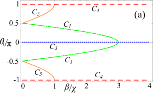
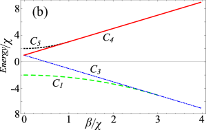
Figure 1: Evolution of the (a) position and (b) energy of the critical points $V_{\cal M}(\theta_{1},\theta_{2},t\leq t_{1})$ as a function of the ratio between the electric field parameter $\beta$ and the dipole-dipole interaction parameter $\chi$.

For $0\leq\beta/\chi<1$, the five equilibria exist. In the field-free case $\beta=0$, the energy surface $V_{\cal M}(\theta_{1},\theta_{2},t\geq t_{1})$ shows the characteristic landscape of the dipole-dipole interaction shown in Fig. 2a. The minima ${\cal C}_{1}$ correspond to the stable head-tail configurations of the dipoles, while the maxima ${\cal C}_{5}$ correspond to the unstable head-head or tail-tail configurations. Thus, if the energy of the system is below the energy of the saddle points ${\cal C}_{2}$, ${\cal E}_{2}=-\chi$, the two dipoles are confined in the potential wells created by the minima ${\cal C}_{1}$ and they oscillate around the stable head-tail configuration. If the energy of the system is larger than ${\cal E}_{2}=-\chi$, and smaller than the energy of the saddle points ${\cal C}_{3}$ and ${\cal C}_{4}$, ${\cal E}_{3}={\cal E}_{4}=\chi$, the oscillations of the dipoles are of large amplitude but still around the stable head-tail configurations. Finally, if the total energy is larger than ${\cal E}_{3}={\cal E}_{4}=\chi$, the rotors can perform complete rotations.

For $0<\beta/\chi<1$, as the ratio $\beta/\chi$ approaches to $1$, the minima ${\cal C}_{1}$ (maxima $C_{5}$) move towards the saddle point $C_{3}$ ($C_{4}$). However, the shape of the energy surface $V_{\cal M}(\theta_{1},\theta_{2},t\geq t_{1})$ remains qualitatively the same, though being somewhat distorted as compared to the field free case, see Fig. 2b for $\beta/\chi=0.9$. As a rough approximation, for $0<\beta/\chi<1$, the interaction due to the electric field could be considered as a perturbation to the dipole-dipole interaction, which dominates the dynamics. For $\beta/\chi=1$, a pitchfork bifurcation takes place between the saddle points $C_{4}$ and the maxima $C_{5}$, see Fig. 1, and from there on only the saddle points $C_{4}$, which become maxima, survive, which is illustrated in Fig. 2c for $\beta/\chi=1.1$. As the electric field parameter increases in the interval $1\leq\beta/\chi<3$, the minima $C_{1}$ keep moving towards $C_{3}$, see Fig. 1 and the contour plot in Fig. 2d for $\beta/\chi=2.9$. At $\beta/\chi=3$, $C_{1}$ and $C_{3}$ collide and a second pitchfork bifurcation occurs. From this bifurcation on, only the critical point $C_{3}$ survives now as minimum, see Fig. 2e for $\beta/\chi=3.1$. For $\beta/\chi\geq 3$, the shape of the energy surface $V_{\cal M}(\theta_{1},\theta_{2},t=t_{1})$ is qualitatively similar to the $\chi=0$ case, where only the interaction due to the electric field is taken into account, cf. Fig. 2e and Fig. 2f. Indeed, for $\beta/\chi\geq 3$, the dipole-dipole interaction could be considered as a perturbation to the electric field interaction.

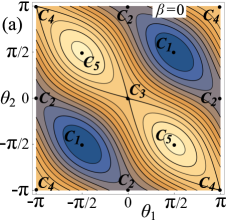
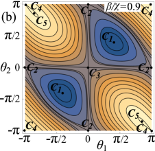
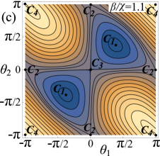
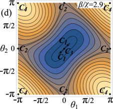
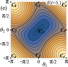
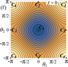
Figure 2: Evolution of the landscape of the potential energy surface $V_{\cal M}(\theta_{1},\theta_{2},t)$ for $t>t_{1}$ and different values of the ratio between the electric field parameter and the dipole-dipole interaction $\beta/\chi$.

II.2 The rotated reference system

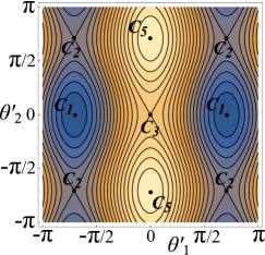
Figure 3: Landscape of the rotated potential energy surface $V^{\prime}(\theta_{1},\theta_{2},t)$ for $\beta=0$ and $t>0$.

A $3\pi/4$ rotation around the axis perpendicular to the plane $(\theta_{1},\theta_{2})$ of the Hamiltonian ((7)) takes the equilibria along the bisector $\theta_{2}=\theta_{1}$ to the axis $\theta_{2}=0$. This rotation is a canonical transformation between the coordinates $(\theta_{1},\theta_{2},P_{1},P_{2})$ and the new ones $(\theta^{\prime}_{1},\theta^{\prime}_{2},P^{\prime}_{1},P^{\prime}_{2})$ given by

$$\theta^{\prime}_{1} = \frac{\theta_{1}+\theta_{2}}{\sqrt{2}},\qquad\theta^{\prime}_{2}=\frac{\theta_{2}-\theta_{1}}{\sqrt{2}},$$ ((10))

$$P^{\prime}_{1} = \frac{P_{1}+P_{2}}{\sqrt{2}},\qquad P^{\prime}_{2}=\frac{P_{2}-P_{1}}{\sqrt{2}},$$

and with generating function ${\cal W}$

$${\cal W}=P^{\prime}_{1}\left(\frac{\theta_{1}+\theta_{2}}{\sqrt{2}}\right)+P^{\prime}_{2}\left(\frac{\theta_{2}-\theta_{1}}{\sqrt{2}}\right).$$ ((11))

The rotated Hamiltonian $H^{\prime}$ reads

$${H}^{\prime}=E^{\prime}=P^{\prime 2}_{1}+P^{\prime 2}_{2}+V^{\prime}_{\cal M}(\theta^{\prime}_{1},\theta^{\prime}_{2},t),$$ ((12))

where

$$V^{\prime}_{\cal M}(\theta^{\prime}_{1},\theta^{\prime}_{2},t) = V^{\prime}_{1}(\theta^{\prime}_{1})+V^{\prime}_{2}(\theta^{\prime}_{1})$$ ((13))

$$- 2\beta f(t)\cos\left(\frac{\theta^{\prime}_{1}}{\sqrt{2}}\right)\cos\left(\frac{\theta^{\prime}_{2}}{\sqrt{2}}\right),$$

with

$$V^{\prime}_{1}(\theta^{\prime}_{1})=\frac{3}{2}\chi\cos(\sqrt{2}\ \theta^{\prime}_{1}),\quad V^{\prime}_{2}(\theta^{\prime}_{2})=-\frac{1}{2}\chi\cos(\sqrt{2}\ \theta^{\prime}_{2}).$$

The potential $V^{\prime}_{\cal M}(\theta^{\prime}_{1},\theta^{\prime}_{2},t)$ represents the potential energy of two pendula coupled by the external electric field.

In the field-free case, $\beta=0$, the dipole-dipole Hamiltonian is separable, ${H}^{\prime}={H}^{\prime}_{1}+{H}^{\prime}_{2}$ with,

$${H}^{\prime}_{1} = E_{1}^{\prime}=P^{\prime 2}_{1}+\frac{3}{2}\chi\cos(\sqrt{2}\ \theta^{\prime}_{1}),$$

$${H}^{\prime}_{2} = E_{2}^{\prime}=P^{\prime 2}_{2}-\frac{1}{2}\chi\cos(\sqrt{2}\ \theta^{\prime}_{2}),$$ ((14))

and the dynamics is that of two uncoupled pendula. The contour plot of $V^{\prime}_{\cal M}(\theta^{\prime}_{1},\theta^{\prime}_{2},t)$ for $\beta=0$ and $t>t_{1}$ is depicted in Fig. 3.

III Energy Transfer in the field-free case

In this section, we explore the energy transfer mechanism between the two field-free rotors assuming that, initially, they do not have the same kinetic energy. Indeed, we assume that initially the two rotors are at rest, with zero kinetic energy, in the bottom of the potential well ${\cal C}_{1}$, i. e., $\theta_{1}=\theta_{2}=\pi/2$, in the stable head-tail configuration with total energy $-2\chi$. Then, a certain amount of kinetic energy $\delta{\cal K}$ is given to the first dipole, in such a way that the initial conditions at $t=0$ are

$$\theta_{1}(0)=\theta_{2}(0)=\frac{\pi}{2},\quad P_{1}(0)=\sqrt{\delta{\cal K}},\quad P_{2}(0)=0.$$ ((15))

With these initial conditions, the Hamiltonian equations of motion (II) for $\beta=0$ are integrated up to a final time $t_{f}$. During the numerical integration, we compute the normalized time average of the kinetic energy of each dipole, $\widehat{P_{i}^{2}}$, given by

$$\widehat{P_{i}^{2}}=\frac{\langle P_{i}^{2}\rangle}{\langle P_{1}^{2}\rangle+\langle P_{2}^{2}\rangle},\quad\langle P_{i}^{2}\rangle=\frac{1}{t_{f}-t_{1}}\int_{t_{1}}^{t_{f}}P_{i}^{2}(t)dt.$$ ((16))

Note that in the field-free case $\beta=0$, and we use $t_{1}=0$. The outcome depends on the parameter of the dipole-dipole interaction $\chi$ and the amount of excess energy $\delta{\cal K}$. Here, we fix the dipole-dipole interaction and investigate the energy transfer as the energy given to the first dipole increases. This dipole-dipole interaction parameter depends on the molecular species, through the rotational constant and permanent electric dipole moment, and on the separation between the dipoles. In this work, we use $\chi=10^{-5}$. In case we were considering the dipoles to be cold LiCs molecules trapped in an optical lattice, the value $\chi=10^{-5}$ would corresponds to an optical lattice with $a_{l}=429$ nm. The parameter $\delta{\cal K}$ is given in units of $\chi$, i. e., in the energy units of the potential energy surface $V_{\cal M}(\theta_{1},\theta_{2},t)$ for $\beta=0$, and we investigate the interval $2\chi\leq\delta{\cal K}\leq 8\chi$. The final time is fixed to $t_{f}=5\times 10^{4}$. Our numerical tests have shown that this value for the stopping time is appropriate for the correct characterization of the outcomes.

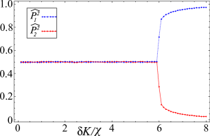
Figure 4: For the field-free system, the normalized time-averaged kinetic energies of the dipoles $\widehat{P_{1}^{2}}$ (blue thick solid line) and $\widehat{P_{2}^{2}}$ (red thin solid line), see Eq. (16), as a function of the initial excess energy of the first molecule $\delta{\cal K}$. The dipole-dipole interaction strength is $\chi=10^{-5}$.

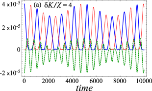
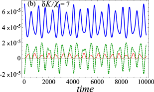
Figure 5: For the field-free system, time-evolution of the kinetic energies $P_{1}^{2}(t)$ (blue thick solid line) and $P_{2}^{2}(t)$ (red thin solid line) and the potential energy $V_{\cal M}(\theta_{1},\theta_{2},t)$ (green dashed line). The initial excess energies of the first molecule are (a) $\delta{\cal K}=4\chi$ and (b) $\delta{\cal K}=7\chi$. The dipole-dipole interaction strength is $\chi=10^{-5}$.

The normalized time-averaged kinetic energies of the dipoles are shown in Fig. 4 as the excess energy $\delta{\cal K}$ increases. If the excess energy $\delta{\cal K}$ is smaller than the critical value $\delta{\cal K}_{c}\approx 6\chi$, the system is in an equipartition energy regime, $\widehat{P_{1}^{2}}$ is very close to $\widehat{P_{2}^{2}}$, and there is a continuous energy flow between the rotors. This behavior is illustrated for $\delta{\cal K}=4\chi$ in Fig. 5a with the time evolution of the kinetic energies $P_{1}^{2}(t)$ and $P_{2}^{2}(t)$, and the potential energy $V_{\cal M}(\theta_{1},\theta_{2},t)$. For $\delta{\cal K}\approx 6\chi$, this equipartition regime abruptly breaks and for $\delta{\cal K}\gtrsim 6\chi$, most of the kinetic energy remains in the first dipole. As a consequence, the energy flow between the dipoles is interrupted as shown in Fig. 5b for $\delta{\cal K}=7\chi$. The dynamics of this first rotor is essentially different in these two regimes. For $\delta{\cal K}<6\chi$, the kinetic energy $P_{1}^{2}(t)$ oscillates and reaches zero as minimal value, see Fig. 5a, which indicates a non continuous rotation and this first dipole is at rest at these minima. For $\delta{\cal K}>6\chi$, $P_{1}^{2}(t)>0$, cf. Fig. 5b, which indicates that the first dipole is performing a continuous rotation. In contrast, the smaller kinetic energy of the second rotor $P_{2}^{2}(t)$ oscillates with a non continuous rotation and has as minimum value zero in both regimes. This behavior in the energy flux between the dipoles was already observed by de Jonge et al. Ratner3 . In that paper, the authors provide an analytical explanation showing that the energy transfer is only possible in a low energy regime.

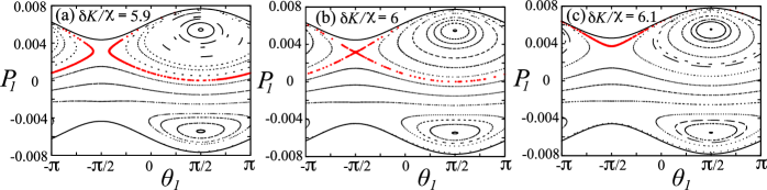
Figure 6: For the field-free system with dipole-dipole interaction $\chi=10^{-5}$, Poincaré surfaces of section in the plane $(P_{1},\theta_{1})$ with $\theta_{2}=\pi/2$ for three different initial excess energies in the neighborhood of the critical value $\delta{\cal K}_{c}=6\chi$. The red thick points correspond to the trajectory $\tau$ with initial conditions ((15)).

To gain a deeper physical insight into the energy transfer mechanism, we present in Fig. 6 the Poincaré surface of section in the plane $(P_{1},\theta_{1})$ with $P_{2}=0$ for three initial excess energies. This surface of section provides a good illustration for the trajectory $\tau$ with initial conditions ((15)). For $\delta{\cal K}_{c}<6\chi$, the orbit $\tau$ has a vibrational nature, see Fig. 6a, whereas we observe in Fig. 6c that its nature becomes rotational for $\delta{\cal K}_{c}>6\chi$. At the critical value $\delta{\cal K}_{c}=6\chi$, the $\tau$ orbit is the separatrix, cf. Fig. 6b, that keeps rotational and vibrational regions away from each other. That is why the transition from the energy equipartition regime to the non-equipartition occurs at the critical value $\delta{\cal K}_{c}=6\chi$.

These energy transfer mechanisms can be explained analyzing the dynamics of the two pendula in the rotated reference frame. The momenta in the LFF and in the rotated frame are related according to

$$P_{1}=\frac{P^{\prime}_{1}-P^{\prime}_{2}}{\sqrt{2}},\qquad P_{2}=\frac{P^{\prime}_{1}+P^{\prime}_{2}}{\sqrt{2}},$$ ((17))

and the time-averaged kinetic energy of each dipole can be written as

$$\langle P_{1}^{2}\rangle=\frac{\langle P^{\prime 2}_{1}\rangle+\langle P^{\prime 2}_{2}\rangle}{2}-\langle P^{\prime}_{1}P^{\prime}_{2}\rangle,$$ ((18))

$$\langle P_{2}^{2}\rangle=\frac{\langle P^{\prime 2}_{1}\rangle+\langle P^{\prime 2}_{2}\rangle}{2}+\langle P^{\prime}_{1}P^{\prime}_{2}\rangle,$$ ((19))

that is, the time-averaged kinetic energies of the dipoles differ by twice the time-average of the product of momenta of the pendula $\langle P^{\prime}_{1}P^{\prime}_{2}\rangle$.

In the rotated reference frame, using the transformations ((10)), the initial conditions $(\theta_{1}(0),P_{1}(0),\theta_{2}(0),P_{2}(0))$ give rise to two (uncoupled) pendular motions governed by the Hamiltonians (II.2) with energies $E_{1}^{\prime}$ and $E_{2}^{\prime}$. These energies determine the motion in the rotated frame, and the kinetic energy transfer mechanism between the rotors. If the energies of the pendula are smaller than the maxima of the potentials $V^{\prime}_{1}(\theta_{1}^{\prime})$ and $V^{\prime}_{2}(\theta_{2}^{\prime})$, i. e., $E_{1}^{\prime}<3\chi/2$ and $E_{2}^{\prime}<\chi/2$, respectively, the total energy of the system is $E=E_{1}^{\prime}+E_{2}^{\prime}<2\chi$, and both pendula describe periodic oscillations, i. e., the momenta $P^{\prime}_{1}$ and $P^{\prime}_{2}$ are periodic functions around zero with $\langle P^{\prime}_{1}\rangle=\langle P^{\prime}_{2}\rangle=0$, and the time-averaged product $\langle P^{\prime}_{1}P^{\prime}_{2}\rangle$ is zero. As a consequence, $\langle P_{1}^{2}\rangle=\langle P_{2}^{2}\rangle$, which means that the system will always belong to the equipartition kinetic energy regime. The same behavior occurs when $E_{1}^{\prime}>3\chi/2$ or $E_{2}^{\prime}>\chi/2$, and at least one of them is in the vibrational regime with $\langle P^{\prime}_{i}\rangle=0$, whereas the other one describes complete periodic rotations and its momentum is a periodic function around a nonzero value having a nonzero time average, and again it holds $\langle P^{\prime}_{1}P^{\prime}_{2}\rangle=0$. Finally, if the initial condition leads to a pendular energy distribution with $E_{1}^{\prime}>3\chi/2$ and $E_{2}^{\prime}>\chi/2$, then, both pendula are in the rotational regime, the time-average product $\langle P^{\prime}_{1}P^{\prime}_{2}\rangle$ is nonzero, and the equipartition regime is not met.

For the orbit $\tau$, the initial conditions ((15)) expressed in the rotated frame read

$$\theta^{\prime}_{1}(0)=\frac{\pi}{\sqrt{2}},\,\theta^{\prime}_{2}(0)=0,\,P^{\prime}_{1}(0)=\sqrt{\frac{\delta{\cal K}}{2}},\,P^{\prime}_{2}(0)=-\sqrt{\frac{\delta{\cal K}}{2}}$$

In this rotated frame, the excess kinetic energies in the pendula are the same, $\delta{\cal K}/2$, whereas their energies are

$$E_{1}^{\prime}=\frac{\delta{\cal K}}{2}-\frac{3}{2}\chi,\qquad E_{2}^{\prime}=\frac{\delta{\cal K}}{2}-\frac{1}{2}\chi.$$ ((20))

If the excess energy satisfies $\delta{\cal K}<2\chi$, both pendula are in an oscillatory motion, and the dipoles belong to the energy equipartition regime. This is illustrated for $\delta{\cal K}=1.8\chi$ in Fig. 7a and Fig. 7b with the time evolution of $P_{1}^{\prime}(t)$, $P_{2}^{\prime}(t)$ and $P_{1}^{\prime}(t)P_{2}^{\prime}(t)$, respectively. If the excess energy satisfies $2\chi<\delta{\cal K}<6\chi$, the second pendulum performs complete rotations, whereas the first one still performs a vibrational motion, see in Fig. 7c and Fig. 7d the evolution of the momenta and the product of momenta for $\delta{\cal K}=5.9\chi$. In this situation, the dipole relaxes again to the equipartition regime. However, if the excess energy is $\delta{\cal K}>6\chi$, both pendula have a rotational motion and the dipoles do not reach the equipartition regime, as an example see for $\delta{\cal K}=6.1\chi$ the time-evolution of the momenta and the product of momenta in Fig. 7e and Fig. 7f.

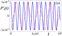
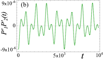
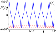
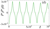
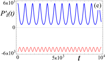
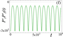
Figure 7: For the field-free system, time evolution of the momenta $P_{1}^{\prime 2}(t)$ (blue thick solid line) and $P_{2}^{\prime 2}(t)$ (red thin solid line) of the uncoupled pendula (upper row) and the product $P^{\prime}_{1}(t)P^{\prime}_{2}(t)$ (green dashed line) (lower row) for the excess energies (a) and (b) $\delta{\cal K}=1.8\chi$; (c) and (d) $\delta{\cal K}=5.9\chi$; (e) and (f) $\delta{\cal K}=6.1\chi$, for $P^{\prime}_{1}(t)$ and $P^{\prime}_{2}$(t), and $P^{\prime}_{1}(t)P^{\prime}_{2}(t)$, respectively. The dipole-dipole interaction strength is $\chi=10^{-5}$.

IV Energy Transfer in an External Electric Field

In this section we explore the energy transfer between the two dipoles in the presence of an external electric field. Again, we assume that the dipoles are initially in the stable head-tail configuration with zero kinetic energy. At time $t=0$, a certain amount of kinetic energy $\delta{\cal K}$ is given to the first dipole, and simultaneously the electric field is turned on with the linear profile ((2)). Using the initial conditions (15), the equations of motion II are integrated up to a final time $t_{f}$, and we compute the normalized time-averaged momenta $\widehat{P}_{1}^{2}$ and $\widehat{P}_{2}^{2}$ from Eq. (16). As in the field-free system, we are using a dipole-dipole interaction with strength $\chi=10^{-5}$, and a final time $t_{f}=5\times 10^{4}$. The strength of the electric field is varied in the interval $0.01\chi\leq\beta\leq 1000\chi$. We assume a switched-on time for the field of $t_{1}=1200$, which roughly corresponds to $100~{}ns$, that could be achieved in current experiments with realistic field strengths.

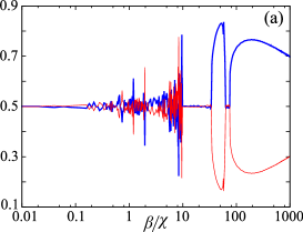
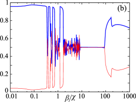
Figure 8: The normalized time-averaged kinetic energies of the dipoles $\widehat{P_{1}}$ (blue thick solid line) and $\widehat{P_{2}}$ (red thin solid line) as a function of the ratio between the electric field parameter $\beta$ and the dipole-dipole parameter $\chi$ for two initial excess energies of the first rotor (a) $\delta{\cal K}=4\chi$ and (b) $\delta{\cal K}=7\chi$. The dipole-dipole interaction parameter is $\chi=10^{-5}$.

Based on the results for the field-free system, we investigate the time-averaged kinetic energies $\widehat{P_{1}^{2}}$ and $\widehat{P_{2}^{2}}$ for $\delta{\cal K}=4\chi$ and $\delta{\cal K}=7\chi$ as the field parameter varies. The results are depicted in Fig. 8. For these two excess energies, $\widehat{P_{1}^{2}}$ and $\widehat{P_{2}^{2}}$ follow essentially different behaviors as $\beta$ increases, but four common patterns can be identified in the two cases of Fig. 8. For small values $\beta\lesssim 0.5\chi$, the dipole-dipole interaction is dominant and adding the external electric field has no relevant effect. As a consequence, we encounter the energy partition regimes for $\delta{\cal K}=4\chi$ (equipartition for $\beta=0$) and $\delta{\cal K}=7\chi$ (non-equipartition for $\beta=0$). By increasing the electric field in the interval $0.5\chi\lesssim\beta\lesssim 10\chi$, the energy partition diagrams show sudden (random) variations. In this field range, the dipole-dipole and electric field interactions are comparable in magnitude and the system dynamics is sensitive to the variations of the the electric field parameter. For intermediate strengths, the dipoles relax to an energy equipartition regime: see $10\chi\lesssim\beta\lesssim 40\chi$ and $10\chi\lesssim\beta\lesssim 100\chi$, for $\delta{\cal K}=4\chi$ and $\delta{\cal K}=7\chi$, respectively. Finally, for stronger electric fields, the system falls out of the equipartition regime, and most of the kinetic energy remains in one of the dipoles. For the initial conditions investigated here, most of the kinetic energy remains in the first dipole. By varying the initial conditions, the role played by the two rotors could change, and the second rotor could store most of the kinetic energy.

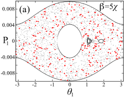
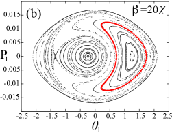
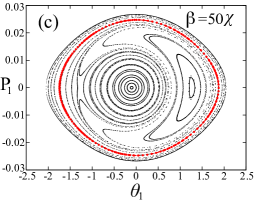
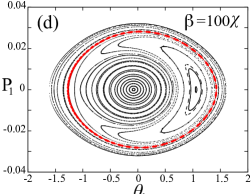
Figure 9: Poincaré surface of section in the plane $(P_{1},\theta_{1})$ with $P_{2}=0$ for different values of the electric field parameter $\beta$. The dipole-dipole interaction is $\chi=10^{-5}$ and the excess kinetic energy of the first dipole is $\delta{\cal K}=4\chi$. The thick (red) points correspond to the trajectory $\tau$ with initial conditions ((15)).

The Poincaré surfaces of section provide a global picture of the phase space structure and are therefore suited to analyze and understand the kinetic energy transfer. We analyze the Poincaré surfaces of section for a fixed $t>t_{1}$, once the electric field parameter has reached its maximal strength $\beta$, and the energy is constant. To illustrate the trajectory $\tau$ with initial conditions ((15)), a suitable surface of section for the Poincaré map is given by the intersection of the phase space trajectories with the plane $(P_{1},\theta_{1})$ with $P_{2}=0$. In Fig. 9 and Fig. 10, we show these Poincaré surfaces of section for different values of the electric field parameter $\beta$ and for the excess energies $\delta{\cal K}=4\chi$ and $\delta{\cal K}=7\chi$, respectively.

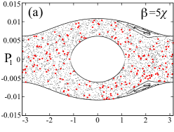
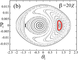
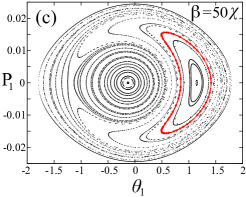
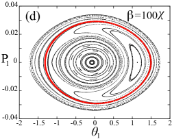
Figure 10: The same as in Fig. 9, but for an excess energy of the first dipole of $\delta{\cal K}=7\chi$.

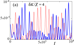
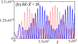
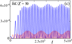
Figure 11: Time evolution of the kinetic energies $P_{1}^{2}(t)$ (thick blue solid line) and $P_{2}^{2}(t)$ (thin red solid line) of the $\tau$ orbit for $\delta{\cal K}=4\chi$ and (a) $\beta=4\chi$, (b) $\beta=20\chi$ and (c) $\beta=50\chi$. The dipole-dipole interaction parameter is to $\chi=10^{-5}$.

For $\beta=5\chi$, the system shows a sensitive dependence on the electric field parameter, cf. Fig. 8, and the Poincaré surfaces of section exhibit a chaotic sea. A single trajectory with initial conditions in this sea covers randomly a large portion of the Poincaré map, see Fig. 9a and Fig. 10a. In particular, the chaotic sea of these surfaces of section results in strongly fluctuating kinetic energies $P_{1}^{2}(t)$ and $P_{2}^{2}(t)$, as it is shown in Fig. 11a for the orbit $\tau$ with $\delta{\cal K}=4\chi$ and $\beta=5\chi$. For stronger electric fields, the phase space of the system is made up of three different types of regular KAM tori organized around two stable periodic orbits, and kept apart by a separatrix attached to an unstable periodic orbit, see Fig. 9 and Fig. 10. Each type of KAM tori corresponds to one of the kinetic energy partition regimes detected in Fig. 8. Indeed, when the dipoles are in the energy equipartition regime, the trajectory $\tau$ falls inside the KAM torus centered around the stable periodic orbit located on the right hand side of the Poincaré surfaces of section. This is observed for the surfaces of section for $\beta=20\chi$ with $\delta{\cal K}=4\chi$ and $\delta{\cal K}=7\chi$ in Fig. 9b and Fig. 10b, respectively, and $\beta=50\chi$ and $\delta{\cal K}=7\chi$ in Fig. 10c. The equipartition energy is manifest in the time evolution of the kinetic energies $P_{1}^{2}(t)$ and $P_{2}^{2}(t)$ presented in Fig. 11b for $\delta{\cal K}=20\chi$ and $\beta=20\chi$. In contrast, if the system falls out of the equipartition regime with the first dipole having most of the kinetic energy, the reference trajectory $\tau$ appears in the corresponding Poincaré maps inside a different type of KAM torus located at the periphery of the Poincaré map, as it is observed for $\beta=50\chi$ and $\delta{\cal K}=4\chi$ in Fig. 9c, and for $\beta=100\chi$ with $\delta{\cal K}=4\chi$ and $\delta{\cal K}=7\chi$ in Fig. 9d and Fig. 10d, respectively. In these orbits, the kinetic energy $P_{1}^{2}(t)$ reaches significantly larger values than $P_{2}^{2}(t)$, see for instance, $P_{1}^{2}(t)$ and $P_{2}^{2}(t)$ shown in Fig. 11c for $\delta{\cal K}=4\chi$ and $\beta=50\chi$. For other values of the excess energy $\delta{\cal K}$, not shown in Fig. 8, the second dipole could have most of the kinetic energy and the corresponding Poincaré surface of section of the trajectory $\tau$ is a KAM torus located around the central stable periodic orbit.

V Conclusions

We have explored the classical phase space and related energy transfer mechanisms between two dipoles in the presence of an homogenous electric field. The dipoles are described by the rigid rotor approximation and are assumed to be fixed in space. In our numerical study, initially the molecules are at rest in the stable lowest energy head-tail configuration. At $t=0$, the system is pushed out of equilibrium by injecting a certain amount of kinetic energy to one of the dipoles. The following dynamics is investigated by analyzing in particular the kinetic energies of the dipoles and their time-averages.

In the field-free case, and depending on the amount of excess energy in one of the dipoles, the system falls to either an energy equipartition regime or a non-equipartition one. The transition between these two regimes is abrupt and takes place at $\delta{\cal K}=6\chi$. The analysis of the phase space structure of the system by means of Poincaré surfaces of section as well as a rotation of the Hamiltonian provide the explanation of this sharp transition.

The impact of the electric field on the energy transfer between the dipoles is quite dramatic. Depending on the field strength, the system shows different behaviors where equipartition, non-equipartition and even chaotic regimes are possible. If the strengths of the dipole-dipole and electric field interactions are comparable, the energy transfer is a chaotic process and the time-averaged kinetic energies strongly depend on the field parameter and show rapid and sudden changes. Again, the phase space structure of the system by means of the Poincaré surfaces of section provides a global picture of the energy exchange mechanism.

We have here been focusing on an invariant subspace of the full dynamics and, therefore, it would be a natural continuation of this work to investigate the exchange of energy in the remaining part of the energy shell. Besides this, an extension of the system to a linear chain of dipoles is of immediate interest.

- (1) Photosynthetic Excitons, H Van Amerongen, L Valkunas, R Van Grondelle, (World Scientific, Singapore, 2000).
- (2) G.S. Engel, T. R. Calhoun, E.L. Read, T.K. Ahn, T. Mancal, Y.C. Cheng, R.E. Blankenship, and G. R. Fleming, Nature 446, 782 (2007).
- (3) Y.-C. Cheng and G. R. Fleming, Annu. Rev. Phys. Chem. 60, 241 (2009).
- (4) J.l. Wu, F. Liu, J. Ma, R. J. Silbey, and J. Cao, J. Chem. Phys. 137, 174111 (2012).
- (5) Energy Transfer Dynamics in Biomaterial Systems, I. Burghardt, V. May, D. A. Micha, and E. R. Bittner (Eds.), (Springer-Verlag Berlin Heidelberg 2009).
- (6) S. K. Saikin, A. Eisfeld, S. Valleau and A. Aspuru-Guzik, Nanophotonics 2, 21 (2013).
- (7) D. Melnikau, D. Savateeva, V. Lesnyak, N. Gaponik, Y. Núnez Fernández, M. I. Vasilevskiy, M. F. Costa, K. E. Mochalov, V. Oleinikov and Y. P. Rakovich, Nanoscale 5, 9317 (2013).
- (8) Y. Qiao, F. Polzer, H. Kirmse, E. Steeg, S. Kühn, S. Friede, S. Kirstein, and J. P. Rabe, ACS Nano 9, 1552 (2015).
- (9) A. S. Davydov, Theory of Molecular Excitons, (New York: McGraw-Hill, 1962).
- (10) R. Silbey, Ann. Rev. Phys. Chem. 27, 203 (1976).
- (11) J. D. Wright, Molecular Crystals, (2nd Edition, Cambridge University Press 1994).
- (12) Cold Molecules: Theory, Experiments and Applications, R. Krems, B. Friedrich and W. C. Stwalley (Eds.), (CRC Press, Taylor & Francis, 2009)
- (13) M. Weidemüller and C. Zimmermann (Ed.), Cold Atoms and Molecules, (Wiley–VCH, 2009).
- (14) T. Lahaye, C. Menotti, L. Santos, M. Lewenstein and T. Pfau, Rep. Prog. Phys. 72, 126401 (2009).
- (15) B. Zhu, J. Schachenmayer, M. Xu, F. H. Urbina, J. G. Restrepo, M. J. Holland, A. M. Rey, New J. Phys. 17, 083063 (2015).
- (16) T. Sowiński, O. Dutta, P. Hauke, L. Tagliacozzo, M. Lewenstein, Phys. Rev. Lett. 108, 115301 (2012).
- (17) S. W. DeLeeuw, D. Solvaeson, M. A. Ratner and J. Michl, J. Phys. Chem. B 102, 3876 (1998).
- (18) E. Sim, M. A. Ratner and S. W. de Leeuw, J. Phys. Chem. B 103, 8663 (1999).
- (19) J. J. de Jonge, M. A. Ratner, S. W. de Leeuw and R. O. Simonis, J. Phys. Chem. B 108, 2666 (2004).
- (20) M. Lemeshko, R. V. Krems, J. M. Doyle, S. Kais, Molecular Physics 111, 1648 (2013).
- (21) E. Fermi, J. Pasta and S. Ulam, Studies of nonlinear problems (Los Alamos document LA-1940, 1955).
- (22) J. Ford, Physics Reports, 213, 271, (1992).
- (23) G. P. Berman and F. M. Izrailev, Chaos, 15, 015104 (2005).
- (24) T. Dauxois, M. Peyrard, and S. Ruffo, Eur. J. Phys. 26, S3 (2005).
- (25) The Fermi-Pasta-Ulam Problem. A Status Report, G. Gallavotti (Eds), (Springer-Verlag Berlin Heidelberg, 2008).
- (26) A. Mussot, A. Kudlinski, M. Droques, P. Szriftgiser, and N. Akhmediev, Phys. Rev. X 4, 011054 (2014).
- (27) D. Bambusi, A. Carati, A. Maiocchi, and A. Maspero, Some Analytic Results on the FPU Paradox, pag. 235, in Hamiltonian Partial Differential Equations and Applications, Fields Institute Communications , P. Guyenne, D. Nicholls and C. Sulem (Eds) (Springer Science+Business Media, New York 2015).
- (28) T. Penati and S. Flach, Chaos 17 023102 (2007).