A Deterministic Mathematical Model for Bidirectional Excluded Flow with Langmuir Kinetics

Abstract

In many important cellular processes, including mRNA translation, gene transcription, phosphotransfer, and intracellular transport, biological “particles” move along some kind of “tracks”. The motion of these particles can be modeled as a one-dimensional movement along an ordered sequence of sites. The biological particles (e.g., ribosomes, RNAPs, phosphate groups, motor proteins) have volume and cannot surpass one another. In some cases, there is a preferred direction of movement along the track, but in general the movement may be two-directional, and furthermore the particles may attach or detach from various regions along the tracks (e.g. ribosomes may drop off the mRNA molecule before reaching a stop codon).

We derive a new deterministic mathematical model for such transport phenomena that may be interpreted as the dynamic mean-field approximation of an important model from mechanical statistics called the asymmetric simple exclusion process (ASEP) with Langmuir kinetics. Using tools from the theory of monotone dynamical systems and contraction theory we show that the model admits a unique equilibrium, and that every solution converges to this equilibrium. This means that the occupancy in all the sites along the lattice converges to a steady-state value that depends on the parameters but not on the initial conditions. Furthermore, we show that the model entrains (or phase locks) to periodic excitations in any of its forward, backward, attachment, or detachment rates.

We demonstrate an application of this phenomenological transport model for analyzing the effect of ribosome drop off in mRNA translation. One may perhaps expect that drop off from a jammed site may increase the total flow by reducing congestion. Our results show that this is not true. Drop off has a substantial effect on the flow, yet always leads to a reduction in the steady-state protein production rate.

I Introduction

Movement is essential for the functioning of cells. Cargoes like organelles and vesicles must be carried between different locations in the cells. The information encoded in DNA and mRNA molecules must be decoded by “biological machines” (RNA polymerases and ribosomes) that move along these molecules in a sequential order.

Many of these important biological transport processes are modeled as the movement of particles along an ordered chain of sites. In the context of intercellular transport, the particles are motor proteins and the chain models actin filaments or microtubules. In transcription, the particles are RNAPs moving along the DNA molecule, and in translation the particles are ribosomes moving along the mRNA molecule (see Figure 1).

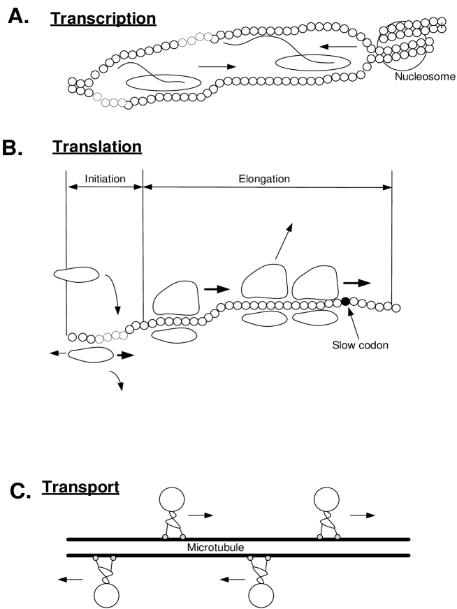
Figure 1: Biological processes that can be studied using the model suggested in this paper.

The movement in such processes may be unidirectional, as in mRNA translation elongation, or bidirectional, as in transcription or translation initiation. Indeed, the normal forward flow of the RNAP may be interrupted, due to transcription errors and various obstacles such as nucleosomes, in which case the RNAP tracks back a few nucleotides and then resumes its normal forward flow [54, 41, 8, 10]. Translation initiation in eukaryotes usually includes diffusion from the 5’end of the transcript towards the start codon [1]. This diffusion process is believed to be bi-directional, but with a preference to the 5’$\to$3’ direction. The movement of motor proteins like kinesin and dynein along microtubules is typically unidirectional, but can be two-directional as well [1].

To increase efficiency, many particles may move simultaneously along the same track thus pipelining the production process. For example, to increase translation efficiency, a number of ribosomes may act simultaneously as polymerases on the same mRNA molecule [66, 4].

The moving biological particles have volume and usually cannot overtake a particle in front of them. This means that a slowly moving particle may lead to the formation of a traffic jam behind it. For example, Leduc et al. [31] have studied Kip3, a yeast kinesin-8 family motor, and demonstrated that motor protein traffic jams can exist, given the right conditions. Other studies have suggested that traffic jams of RNAP [ribosomes] may evolve during transcription [translation] [4, 27, 9].

In some of these biological transport processes, the biological machines may either attach or detach at various sites along the tracks. For example, ribosomes may detach from the mRNA molecule before reaching the stop codon due to traffic “jams” and ribosome-ribosome interactions or due to depletion in the concentration of tRNAs [72, 28, 57]. Also, it is known that kinesin-family motor proteins are more susceptible to dissociation when their pathway is blocked [14, 62].

Defects in these transport processes may lead to severe diseases or may even be lethal. For example, [53] lists the implications of malfunctions of protein motors in disease and developmental defects.

Developing a better understanding of these dynamical biological processes by combining mathematical modeling and biological experiments will have far reaching implications to basic science in fields such as molecular evolution and functional genomics, as well as applications in synthetic biology, biotechnology, human health, and more. Mathematical or computational modeling is especially important in developing approaches for manipulating and controlling these processes, e.g. in order to optimize various goals in biotechnology.

A standard model for such transport processes is the asymmetric simple exclusion process (ASEP) [55, 73]. This is a stochastic model describing particles that hop along an ordered lattice of sites. Each site can be either empty or occupied by a single particle, and a particle can only hop to an empty site. This “simple exclusion principle” represents the fact that the particles have volume and cannot overtake one another. Simple exclusion generates an indirect coupling between the particles. In particular, traffic jams may develop behind a slow-moving particle.

In ASEP, a particle may hop to any of the two neighboring sites (but only if they are free). Typically, a particle can attach the lattice in one of its ends and detach from the other end. When particles can also attach or detach at internal sites along the lattice, the model is referred to as ASEP with Langmuir kinetics. In the special case where the hops are unidirectional, ASEP is sometimes referred to as the totally asymmetric simple exclusion process (TASEP). A TASEP-like system with Langmuir kinetics has been used to model limit order markets in [65], and is often used in modeling molecular motor traffic [42, 43, 32, 33, 16]. More generally, ASEP has become a fundamental model in non-equilibrium statistical mechanics, and has been applied to model numerous natural and artificial processes including traffic and pedestrian flow, the movement of ants, evacuation dynamics, and more [52].

In this paper, we introduce a deterministic mathematical model that may be interpreted as the dynamic mean-field approximation of ASEP with Langmuir kinetics (MFALK). We analyze the MFALK using tools from systems and control theory. In particular, we apply some recent developments in contraction theory to prove that the model is globally asymptotically stable, and that it entrains to periodic excitations in the transition/attachment/detachment rates. In other words, if these rates change periodically in time with some common period $T$ then all the state-variables in the MFALK converge to a periodic solution with period $T$. This is important because many biological processes are excited by periodic signals (e.g. the 24h solar day or the periodic cell-division process), and proper functioning requires phase-locking or entrainment to these excitations.

Our work is motivated by the analysis of a model for mRNA translation called the ribosome flow model (RFM) [48]. This is the mean-field approximation of the unidirectional TASEP without Langmuir kinetics (see, e.g., [52, section 4.9.7] and [6, p. R345]). Recently, the RFM has been studied extensively using tools from systems and control theory [36, 71, 37, 38, 35, 44, 45, 47, 70]. The analysis is motivated by implications to many important biological questions. For example, the sensitivity of the protein production rate to the initiation and elongation rates along the mRNA molecule [45], maximization of protein production rate [44], the effect of ribosome recycling [38, 47], and the consequences of competition for ribosomes on large-scale simultaneous mRNA translation in the cell [46] (see also [19, 2] for some related models).

The MFALK presented here is much more general than the RFM, and can thus be used to model and analyze many transport phenomena, including all the biological processes mentioned above, that cannot be captured using the RFM. We demonstrate this by using the MFALK to model and analyze mRNA translation with ribosome drop off - a feature that cannot be modeled using the RFM.

Ribosome drop off is a fundamental phenomena that has received considerable attention (see, e.g., [57, 25, 24, 68, 7, 61, 18, 28, 22, 20]). In many cases, ribosome drop off is deleterious to the cell since translation is the most energetically consuming process in the cell and, furthermore, drop off yields truncated, non-functional proteins. Thus, transcripts undergo selection to minimize drop off or its energetic cost [67, 63, 61, 18, 28, 20]. There are various hypotheses on the biological advantages of ribosome drop off. For example, Zaher and Green [69] have suggested that ribosome drop off is related to proof reading. One may perhaps expect that another advantage is that drop off from a jammed site may increase the total flow by reducing congestion. Our results using analysis of the MFALK show that this is not true. Drop off has a substantial effect on the flow, yet it always leads to a reduction in the steady-state protein production rate.

The remainder of this paper is organized as follows. The next section describes the new mathematical model. Section III presents our main analysis results. Section IV describes the application of the MFALK to model mRNA translation with ribosome drop off. The final section concludes and describes possible directions for further research. To streamline the presentation, all the proofs are placed in the Appendix.

II The model

The MFALK is a set of $n$ first-order nonlinear differential equations, where $n$ denotes the number of compartments or sites along the “track”. Each site is associated with a state variable $x_{i}(t)\in[0,1]$ describing the normalized “level of occupancy” at site $i$ at time $t$, with $x_{i}(t)=0$ [$x_{i}(t)=1$] representing that site $i$ is completely free [full] at time $t$. Since $x_{i}(t)\in[0,1]$ for all $t$, it may also be interpreted as the probability that site $i$ is occupied at time $t$.

The MFALK contains four sets of non-negative parameters:

• $\lambda_{i}$, $i=0,\dots,n$, controls the forward transition rate from site $i$ to site $i+1$,

• $\gamma_{i}$, $i=0,\dots,n$, controls the backward transition rate from site $i+1$ to site $i$,

• $\beta_{i}$, $i=1,\dots,n$, controls the attachment rate to site $i$,

• $\alpha_{i}$, $i=1,\dots,n$, controls the detachment rate from site $i$,

where we arbitrarily refer to left-to-right flow along the chain as forward flow, and to flow in the other direction as backward flow.

The dynamical equations describing the MFALK are:

$$\dot{x}_{1} =\lambda_{0}(1-x_{1})+\gamma_{1}x_{2}(1-x_{1})+\beta_{1}(1-x_{1})-\lambda_{1}x_{1}(1-x_{2})-\gamma_{0}x_{1}-\alpha_{1}x_{1},$$

$$\dot{x}_{2} =\lambda_{1}x_{1}(1-x_{2})+\gamma_{2}x_{3}(1-x_{2})+\beta_{2}(1-x_{2})-\lambda_{2}x_{2}(1-x_{3})-\gamma_{1}x_{2}(1-x_{1})-\alpha_{2}x_{2},$$

$$\vdots$$

$$\dot{x}_{n-1} =\lambda_{n-2}x_{n-2}(1-x_{n-1})+\gamma_{n-1}x_{n}(1-x_{n-1})+\beta_{n-1}(1-x_{n-1})-\lambda_{n-1}x_{n-1}(1-x_{n})$$

$$-\gamma_{n-2}x_{n-1}(1-x_{n-2})-\alpha_{n-1}x_{n-1},$$

$$\dot{x}_{n} =\lambda_{n-1}x_{n-1}(1-x_{n})+\gamma_{n}(1-x_{n})+\beta_{n}(1-x_{n})-\lambda_{n}x_{n}-\gamma_{n-1}x_{n}(1-x_{n-1})-\alpha_{n}x_{n}.$$ (1)

To explain these equations, consider for example the equation for the change in the occupancy in site $2$, namely,

$$\dot{x}_{2}=\lambda_{1}x_{1}(1-x_{2})+\gamma_{2}x_{3}(1-x_{2})+\beta_{2}(1-x_{2})-\lambda_{2}x_{2}(1-x_{3})-\gamma_{1}x_{2}(1-x_{1})-\alpha_{2}x_{2}.$$

The term $\lambda_{1}x_{1}(1-x_{2})$ represents the flow from site $1$ to site $2$. This increases with the occupancy in site $1$, and decreases with the occupancy in site $2$. In particular, this term becomes zero when $x_{2}=1$, i.e. when site $2$ is completely full. This is a “soft” version of the hard exclusion principle in ASEP: the effective entry rate into a site decreases as it becomes fuller. Note that the constant $\lambda_{1}\geq 0$ describes the maximal possible transition rate from site $1$ to site $2$. Similarly, the term $\lambda_{2}x_{2}(1-x_{3})$ represents the flow from site $2$ to site $3$. The term $\gamma_{2}x_{3}(1-x_{2})$ [$\gamma_{1}x_{2}(1-x_{1})$] represents the backward flow from site $3$ to site $2$ [site $2$ to site $1$]. Note that these terms also model soft exclusion. The term $\beta_{2}(1-x_{2})$ represents attachment of particles from the environment to site $2$, whereas $\alpha_{2}x_{2}$ represents detachment of particles from site $2$ to the environment (see Fig. 2).

The MFALK is a compartmental model [21, 51], as every state-variable describes the occupancy in a compartment (e.g., a site along the the mRNA, gene, microtubule), and the dynamical equations describe the flow between these compartments and the environment. Compartmental models play an important role in pharmacokinetics, enzyme kinetics, basic nutritional processes, cellular growth, and pathological processes, such as tumourigenesis and atherosclerosis (see, e.g., [21, 17] and the references therein). More specifically, the MFALK is a nonlinear tridiagonal compartmental model, as every $\dot{x}_{i}$ directly depends on $x_{i-1},x_{i}$, and $x_{i+1}$ only.

Note also that

$$\sum_{i=1}^{n}\dot{x}_{i} =\lambda_{0}(1-x_{1})-\gamma_{0}x_{1}+\beta_{1}(1-x_{1})-\alpha_{1}x_{1}$$

$$+\gamma_{n}(1-x_{n})-\lambda_{n}x_{n}+\beta_{n}(1-x_{n})-\alpha_{n}x_{n}$$

$$+\sum_{i=2}^{n-1}(\beta_{i}(1-x_{i})-\alpha_{i}x_{i}).$$ (2)

The term on the right-hand side of the first [second] line here represents the change in $x_{0}$ [$x_{n}$] due to the flow between the environment and site $1$ [site $n$], whereas the term on the third line represents the flow between internal sites and the environment.

Figure 2: Topology of the MFALK.

The output rate from site $n$ at time $t$ is the total flow from this site to the environment:

$$R(t): =(\lambda_{n}+\alpha_{n})x_{n}(t)-(\gamma_{n}+\beta_{n})(1-x_{n}(t)).$$ (3)

Note that $R(t)$ may be positive, zero, or negative.

In the particular case where $\alpha_{i}=\beta_{i}=\gamma_{i}=0$ for all $i$ the MFALK becomes the RFM, i.e. the dynamic mean-field approximation of the unidirectional TASEP with open boundary conditions and without Langmuir kinetics.

Let $x(t,a)$ denote the solution of (II) at time $t\geq 0$ for the initial condition $x(0)=a$. Since the state-variables correspond to normalized occupancy levels, we always assume that $a$ belongs to the closed $n$-dimensional unit cube:

$$C^{n}:=\{x\in\mathbb{R}^{n}:x_{i}\in[0,1],i=1,\dots,n\}.$$

Let $\operatorname{{\mathrm{i}nt}}(C^{n})$ denote the interior of $C^{n}$, and let $\partial C^{n}$ denote the boundary of $C^{n}$. The next section analyzes the MFALK defined in (II).

III Main Results

III-A Invariance and persistence

It is straightforward to show that $C^{n}$ is an invariant set for the dynamics of the MFALK, that is, if $a\in C^{n}$ then $x(t,a)\in C^{n}$ for all $t\geq 0$. The following result shows that a stronger property holds. Recall that all the proofs are placed in the Appendix. For notational convenience, let $\alpha_{0}:=0$, $\gamma_{0}:=0$, $\alpha_{n+1}:=0$, and $\beta_{n+1}:=0$.

Proposition 1

Suppose that at least one of the following two conditions holds:

$$\lambda_{i}+\beta_{i+1}>0,\quad\text{for all }i\in\{0,\dots,n\},$$ (4)

or

$$\gamma_{i}+\alpha_{i+1}>0,\quad\text{for all }i\in\{0,\dots,n\}.$$ (5)

Then for any $\tau>0$ there exists $d=d(\tau)\in(0,1/2]$ such that

$$d\leq x_{i}(t+\tau,a)\leq 1-d,$$ (6)

for all $a\in C^{n}$, all $i\in\{1,\dots,n\}$, and all $t\geq 0$.

This means in particular that trajectories that emanate from the boundary of $C^{n}$ “immediately” enter $C^{n}$. This result is useful because as we will see below on the boundary of $C^{n}$ the MFALK looses some important properties. For example, the Jacobian matrix of the dynamics (II) is irreducible on $\operatorname{{\mathrm{i}nt}}(C^{n})$, but becomes reducible on some points on the boundary of $C^{n}$.

III-B Contraction

Differential analysis and in particular contraction theory proved to be a powerful tool for analyzing nonlinear dynamical systems. In a contractive system, trajectories that emanate from different initial conditions contract to each other at an exponential rate [34, 49, 3]. Let $|\cdot|_{1}:\mathbb{R}^{n}\to\mathbb{R}_{+}$ denote the $L_{1}$ norm, i.e. for $z\in\mathbb{R}^{n}$, $|z|_{1}=|z_{1}|+\dots+|z_{n}|$.

Proposition 2

Let

$$\eta:=\max\{-\lambda_{0}-\gamma_{0}-\alpha_{1}-\beta_{1},-\alpha_{2}-\beta_{2},\dots,-\alpha_{n-1}-\beta_{n-1},-\lambda_{n}-\gamma_{n}-\alpha_{n}-\beta_{n}\}.$$

Note that $\eta\leq 0$. For any $a,b\in C^{n}$ and any $t\geq 0$,

$$|x(t,a)-x(t,b)|_{1}\leq\exp(\eta t)|a-b|_{1}.$$ (7)

This implies that the $L_{1}$ distance between any two trajectories contracts with the exponential rate $\eta$. Roughly speaking, this also means that increasing all the sums $\alpha_{i}+\beta_{i}$, $i=1,\dots,n$, makes the system “more contractive”. Indeed, these parameters have a direct stabilizing effect on the dynamics of site $i$, whereas the other parameters affect the site indirectly via the coupling to the two adjacent sites.

When $\eta=0$, (7) only implies that the $L_{1}$ distance between trajectories does not increase. This property is not strong enough to prove the asymptotic properties described in the subsections below. Indeed, in this case it is possible that the MFALK will not be contractive with respect to any fixed norm. Fortunately, a certain generalization of contraction turns out to hold in this case.

Consider the time-varying dynamical system

$$\dot{x}(t)=f(t,x(t)),$$ (8)

whose trajectories evolve on a compact and convex set $\Omega\subset\mathbb{R}^{n}$. Let $x(t,t_{0},a)$ denote the solution of (8) at time $t$ for the initial condition $x(t_{0})=a$. System (8) is said to be contractive after a small overshoot (SO) [39] on $\Omega$ w.r.t. a norm $|\cdot|:\mathbb{R}^{n}\to\mathbb{R}_{+}$ if for any $\varepsilon>0$ there exists $\ell=\ell(\varepsilon)>0$ such that

$$|x(t,t_{0},a)-x(t,t_{0},b)|\leq(1+\varepsilon)\exp(-\ell t)|a-b|,$$

for all $a,b\in\Omega$ and all $t\geq t_{0}\geq 0$. Intuitively speaking, this means contraction with an exponential rate, but with an arbitrarily small overshoot of $1+\varepsilon$.

Proposition 3

Suppose that

$$\lambda_{i}+\gamma_{i}>0,\quad\text{for all }i\in\{1,\dots,n-1\},$$ (9)

and that at least one of the two conditions (4), (5) holds. Then the MFALK is SO on $C^{n}$ w.r.t. the $L_{1}$ norm, that is, for any $\varepsilon>0$ there exists $\ell=\ell(\varepsilon)>0$ such that

$$|x(t,a)-x(t,b)|_{1}\leq(1+\varepsilon)\exp(-\ell t)|a-b|_{1},$$ (10)

for all $a,b\in C^{n}$ and all $t\geq 0$.

Note that if $\lambda_{i}+\gamma_{i}=0$ for some $i\in\{1,\dots,n-1\}$, that is $\lambda_{i}=\gamma_{i}=0$, then the MFALK decouples into two separate MFALKs: one containing sites $1,\dots,i$, and the other containing sites $i+1,\dots,n$. Thus, assuming (9) incurs no loss of generality.

There is an important difference between Propositions 2 and 3. If $\eta<0$ then Proposition 2 provides an explicit exponential contraction rate. If $\eta=0$ then Proposition 3 can be used to deduce SO, but in this result the contraction rate $\ell$ depends on $\varepsilon$ and is not given explicitly.

The contraction results above imply that the MFALK satisfies several important asymptotic properties. These are described in the following subsections.

III-C Global asymptotic stability

Since the compact and convex set $C^{n}$ is an invariant set of the dynamics, it contains an equilibrium point $e$. By Proposition 1, $e\in\operatorname{{\mathrm{i}nt}}(C^{n})$. Applying (10) with $b=e$ yields the following result.

Corollary 1

Suppose that the conditions in Proposition 3 hold. Then the MFALK admits a unique equilibrium point $e\in\operatorname{{\mathrm{i}nt}}(C^{n})$ that is globally asymptotically stable, i.e. $\lim_{t\to\infty}x(t,a)=e$, for all $a\in C^{n}$.

This means that the rates determine a unique distribution profile along the lattice, and that all trajectories emanating from different initial conditions in $C^{n}$ asymptotically converge to this distribution. In addition, perturbations in the occupancy levels along the sites will not change this asymptotic behavior of the dynamics. This also means that various numerical solvers of ODEs will work well for the MFALK (see e.g. [13]).

Example 1

Fig. 3 depicts the trajectories of a MFALK with $n=3$, $\lambda_{0}=1.0$, $\lambda_{1}=1.2$, $\lambda_{2}=0.8$, $\lambda_{3}=0.9$, $\gamma_{i}=\lambda_{i}-0.3$, $i=0,\dots,3$, $\alpha_{1}=0$, $\alpha_{2}=0.1$, $\alpha_{3}=0$, $\beta_{1}=0$, $\beta_{2}=0.2$, $\beta_{3}=0$, for six initial conditions in $C^{n}$. It may be seen that all trajectories converge to an equilibrium point $e\in\operatorname{{\mathrm{i}nt}}(C^{3})$.  $\square$

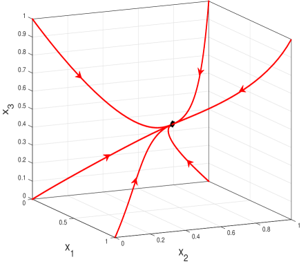
Figure 3: Trajectories of the MFALK in Example 1 for six initial conditions in $C^{3}$.

The MFALK (II) can be written as

$$\dot{x}_{i}=f_{i-1}(x)-f_{i}(x)+g_{i}(x_{i}),\quad i=1,\dots,n,$$ (11)

where

$$f_{0}(x) :=\lambda_{0}(1-x_{1})-\gamma_{0}x_{1},$$

$$f_{i}(x) :=\lambda_{i}x_{i}(1-x_{i+1})-\gamma_{i}x_{i+1}(1-x_{i}),\quad i=1,\dots,n-1,$$

$$f_{n}(x) :=\lambda_{n}x_{n}-\gamma_{n}(1-x_{n}),$$

$$g_{i}(x_{i}) :=\beta_{i}(1-x_{i})-\alpha_{i}x_{i},\quad i=1,\dots,n.$$ (12)

At steady-state, i.e. for $x=e$, the left-hand side of all the equations in (11) is zero, so

$$f_{i-1}(e)=f_{i}(e)-g_{i}(e_{i}),\quad i=1,\dots,n.$$ (13)

Let $v:=\begin{bmatrix}\alpha_{1},\dots,\alpha_{n},\beta_{1},\dots,\beta_{n},\gamma_{0},\dots,\gamma_{n},\lambda_{0},\dots,\lambda_{n}\end{bmatrix}^{\prime}\in\mathbb{R}^{4n+2}_{+}$ denote the parameters of the MFALK. It follows from (13) that if we multiply all these parameters by $c>0$ then $e$ will not change, that is, $e(cv)=e(v)$. Let

$$R:=(\lambda_{n}+\alpha_{n})e_{n}-(\gamma_{n}+\beta_{n})(1-e_{n}),$$ (14)

denote the steady-state output rate. Then $R(cv)=cR(v)$, for all $c>0$, that is, the steady-state production rate is homogeneous of order one w.r.t. the parameters. By (13),

$$R =f_{n}(e)-g_{n}(e_{n})$$

$$=f_{i}(e)+\sum_{j=i+1}^{n-1}g_{j}(e_{j}),\quad i=0,\dots,n-1.$$ (15)

This yields the following set of recursive equations relating the steady-state occupancy levels and the output rate in the MFALK:

$$e_{n} =\frac{R+\gamma_{n}+\beta_{n}}{\lambda_{n}+\gamma_{n}+\beta_{n}+\alpha_{n}},$$

$$e_{i} =\frac{R+\gamma_{i}e_{i+1}-\sum_{j=i+1}^{n-1}g_{j}(e_{j})}{\lambda_{i}(1-e_{i+1})+\gamma_{i}e_{i+1}},\quad i=n-1,\dots,1,$$ (16)

and also

$$e_{1} =\frac{\lambda_{0}+\beta_{1}-R+\sum_{j=2}^{n-1}g_{j}(e_{j})}{\lambda_{0}+\gamma_{0}+\beta_{1}+\alpha_{1}}.$$

For a given $v$, this is a set of $n+1$ equations in the $n+1$ unknowns: $e_{1},\dots,e_{n},R$.

Example 2

Consider the MFALK with dimension $n=2$. Then (III-C) becomes

$$e_{2} =\>\frac{R+\gamma_{2}+\beta_{2}}{\lambda_{2}+\gamma_{2}+\alpha_{2}+\beta_{2}},$$

$$e_{1} =\;\frac{R+\gamma_{1}e_{2}}{\lambda_{1}(1-e_{2})+\gamma_{1}e_{2}},$$ (17)

and also

$$e_{1} =\;\frac{\lambda_{0}+\beta_{1}-R}{\lambda_{0}+\gamma_{0}+\beta_{1}+\alpha_{1}}.$$

This yields the polynomial equation $a_{2}R^{2}+a_{1}R+a_{0}=0$, where

$$a_{2} :=\lambda_{1}-\gamma_{1},$$

$$a_{1} :=(\lambda_{1}-\gamma_{1})(\gamma_{2}+\beta_{2}-\lambda_{0}-\beta_{1})-\lambda_{1}z_{2}-z_{1}z_{2}-z_{1}\gamma_{1},$$

$$a_{0} :=(\lambda_{0}+\beta_{1})\lambda_{1}(\lambda_{2}+\alpha_{2})-(\gamma_{0}+\alpha_{1})\gamma_{1}(\gamma_{2}+\beta_{2}),$$

with $z_{1}:=\lambda_{0}+\gamma_{0}+\alpha_{1}+\beta_{1}$ and $z_{2}:=\lambda_{2}+\gamma_{2}+\alpha_{2}+\beta_{2}$.

Note that the polynomial equation admits several solutions $R$, but only one solution corresponds to the unique equilibrium point $e\in C^{2}$. For example, for $\lambda_{i}=1$, $\gamma_{i}=2$, $\beta_{i}=3$, and $\alpha_{i}=4$ for all $i$ the polynomial equation becomes $-R^{2}-131R-40=0$. This admits two solutions $R_{1}=(-3s-131)/2$ and $R_{2}=(3s-131)/2$, with $s:=\sqrt{1889}$. Substituting $R_{1}$ in (2) yields $e=[e_{1}\;e_{2}]^{\prime}$, with $e_{2}<0$, so this is not a feasible solution. Substituting $R_{2}$ in (2) yields (all numbers are to four digit accuracy) $e=\begin{bmatrix}0.4305&0.4695\end{bmatrix}^{\prime}\in C^{2}$, which is the unique feasible solution. Thus, the steady-state output rate is $R_{2}=-0.3046$.  $\square$

In general, (III-C) can be transformed into a polynomial equation for $R$. The next result shows that the degree of this polynomial equation grows quickly with $n$.

Proposition 4

Consider the MFALK with dimension $n$ and with $\lambda_{i}\neq\gamma_{i}$, $\alpha_{i}\neq 0$, $\beta_{i}\neq 0$, for all $i$. Then generically Eq. (III-C) may be written as $w(R)=0$, where $w(R)$ is a polynomial equation in $R$ of degree $1+\lfloor\frac{2^{n}}{3}\rfloor$, and with coefficients that are algebraic functions of the rates.

We note that this is exponential increase in the degree of the polynomial equation is a feature of the MFALK that does not take place in the RFM. Indeed, in the RFM the degree of the polynomial equation for the steady-state production rate grows linearly with $n$.

Let $\operatorname{{\mathrm{s}gn}}(\cdot):\mathbb{R}\to\{-1,0,1\}$ denote the sign function, i.e.

$$\operatorname{{\mathrm{s}gn}}(y)=\begin{cases}1,&y>0,\\ 0,&y=0,\\ -1,&y<0.\end{cases}$$

An interesting question is what is $\operatorname{{\mathrm{s}gn}}(R)$. Indeed, if this is positive (negative) then this means that there is a net steady-state flow from left to right (right to left). The next subsection describes a special case where this question can be answered rigorously.

III-C1 Bidirectional flow with no Langmuir kinetics

In the case where $\beta_{i}=\alpha_{i}=0$, $i=1,\dots,n$, i.e. a system with no internal attachments and detachments, Eq. (III-C) becomes

$$R=f_{i}(e),\quad i=0,\dots,n.$$ (18)

Proposition 5

Consider the case where $\alpha_{i}=\beta_{i}=0$, $i=1,\dots,n$, and suppose that (9) holds. Then

$$\operatorname{{\mathrm{s}gn}}(R)=\operatorname{{\mathrm{s}gn}}\left(\prod_{i=0}^{n}\lambda_{i}-\prod_{i=0}^{n}\gamma_{i}\right).$$ (19)

In particular, if $\prod_{i=0}^{n}\lambda_{i}=\prod_{i=0}^{n}\gamma_{i}$ then $R=0$, and

$$e_{i}=\frac{\prod_{j=0}^{i-1}\lambda_{j}}{\prod_{j=0}^{i-1}\lambda_{j}+\prod_{j=0}^{i-1}\gamma_{j}}=\frac{\prod_{j=i}^{n}\gamma_{j}}{\prod_{j=i}^{n}\gamma_{j}+\prod_{j=i}^{n}\lambda_{j}},\quad i=1,\dots,n.$$ (20)

Eq. (19) means that in the case of no Langmuir kinetics the steady-state output from the right hand-side of the chain will be positive [negative] if the the product of the forward rates is larger [smaller] than the product of the backward rates. In transcription and translation the steady state flow from the right hand-side of the chain should always be positive, but in other cases, e.g. transport along microtubules, the steady state flow may be either positive or negative.

III-D Entrainment

Assume now that some or all of the rates are time-varying periodic functions with the same period $T$. This may be interpreted as a periodic excitation of the system. Many biological processes are affected by such excitations due for example to the periodic 24h solar day or the periodic cell-cycle division process. For example, translation elongation factors, tRNAs, translation and transcription initiation factors, ATP levels, and more may change in a periodic manner and affect various rates that appear in the MFALK.

A natural question is will the state-variables of the MFALK converge to a periodic pattern with period $T$? We will show that this is indeed so, i.e. the MFALK entrains to a periodic excitation in the rates. In order to understand what this means, consider a different setting, namely, using the MFALK to model traffic flow. Then the rates may correspond to traffic lights, changing in a periodic manner, and the state-variables are the density of the moving particles (cars) along different sections of the road, so entrainment corresponds to what is known as the “green wave” (see e.g. [26] and the references therein).

We say that a function $f$ is $T$-periodic if $f(t+T)=f(t)$ for all $t$. Assume that the $\lambda_{i}$s, $\gamma_{i}$s, $\alpha_{i}$s and $\beta_{i}$s are uniformly bounded, non-negative, time-varying functions satisfying:

• there exists a (minimal) $T>0$ such that all the $\lambda_{i}(t)$s, $\gamma_{i}(t)$s, $\alpha_{i}(t)$s, and $\beta_{i}(t)$s are $T$-periodic.

• there exist $c_{1},c_{2}>0$ such that at least one of the following two conditions holds for all time $t$

  $$\lambda_{i}(t)+\beta_{i+1}(t) >c_{1},\quad i=0,\dots,n,$$ (21)

  $$\gamma_{i}(t)+\alpha_{i+1}(t) >c_{2},\quad i=0,\dots,n.$$ (22)

• there exists $c_{3}>0$ such that

  $$\lambda_{i}(t)+\gamma_{i+1}(t) >c_{3},\quad i=0,\dots,n.$$ (23)

We refer to this model as the Periodic MFALK (PMFALK).

Theorem 1

Consider the PMFALK with dimension $n$. There exists a unique function $\phi(\cdot):\mathbb{R}_{+}\to\operatorname{{\mathrm{i}nt}}(C^{n})$, that is $T$-periodic, and for any $a\in C^{n}$ the trajectory $x(t,a)$ converges to $\phi$ as $t\to\infty$.

Thus, the PMFALK entrains (or phase-locks) to the periodic excitation in the parameters. In particular, this means that the output rate $R(t)$ in (3) converges to the unique $T$-periodic function:

$$(\lambda_{n}(t)+\gamma_{n}(t)+\beta_{n}(t)+\alpha_{n}(t))\phi_{n}(t)-\gamma_{n}(t)-\beta_{n}(t).$$

Note that since a constant function is a periodic function for all $T\geq 0$, Theorem 1 implies that entrainment holds also in the particular case where a single parameter is oscillating (with period $T>0$), while all other parameters are constant. Note also that Corollary 1 follows from Theorem 1.

Example 3

Consider the MFALK with dimension $n=3$, parameters: $\lambda_{0}(t)\equiv 1.0$, $\lambda_{1}(t)\equiv 1.2$, $\lambda_{2}(t)=1+0.5\sin(\pi t/4)$, $\lambda_{3}(t)\equiv 0.9$, $\gamma_{0}(t)\equiv 0.4$, $\gamma_{1}(t)=0.4(1+\sin((\pi t/4)+1/2))$, $\gamma_{2}(t)\equiv 0.25$, $\gamma_{3}(t)\equiv 0.45$, $\alpha_{1}(t)\equiv 0$, $\alpha_{2}(t)\equiv 0.05$, $\alpha_{3}(t)\equiv 0$, $\beta_{1}(t)\equiv 0$, $\beta_{2}(t)=0.05(1+\sin((\pi t/2)+1/4))$, $\beta_{3}(t)\equiv 0$, and initial condition $x(0)=\begin{bmatrix}0.8&0.8&0.8\end{bmatrix}^{\prime}$. Note that all the rates here are periodic, with a minimal common period $T=8$. Fig. 4 depicts $x_{i}(t)$, $i=1,2,3$, as a function of $t$. It may be seen that each state variable converges to a periodic function with period $T=8$.  $\square$

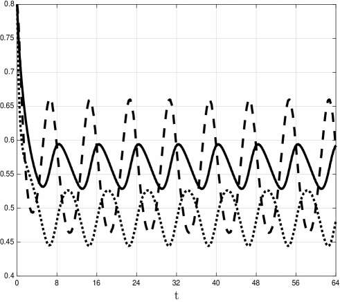
Figure 4: State variables $x_{1}(t)$ [solid line]; $x_{2}(t)$ [dashed line]; and $x_{3}(t)$ [dotted line] as a function of $t$ in Example 3. Note that each state variable converges to a periodic function with a period $T=8$.

III-E Strong Monotonicity

Recall that a proper cone $K\subseteq\mathbb{R}^{n}$ defines a partial ordering in $\mathbb{R}^{n}$ as follows. For two vectors $a,b\in\mathbb{R}^{n}$, we write $a\leq b$ if $(b-a)\in K$; $a<b$ if $a\leq b$ and $a\not=b$; and $a\ll b$ if $(b-a)\in\operatorname{{\mathrm{i}nt}}(K)$. The system $\dot{y}=f(y)$ is called monotone if $a\leq b$ implies that $y(t,a)\leq y(t,b)$ for all $t\geq 0$. In other words, the flow preserves the partial ordering [60]. It is called strongly monotone if $a<b$ implies that $y(t,a)\ll y(t,b)$ for all $t>0$.

From here on we consider the particular case where the cone is $K:=\mathbb{R}^{n}_{+}$. Then $a\leq b$ if $a_{i}\leq b_{i}$ for all $i$, and $a\ll b$ if $a_{i}<b_{i}$ for all $i$. A system that is monotone with respect to this partial ordering is called cooperative.

Proposition 6

For any $a,b\in C^{n}$, with $a\leq b$, the solutions of the MFALK satisfy

$$x(t,a)\leq x(t,b),\quad\text{for all }t\geq 0.$$ (24)

Furthermore, if (9) holds then

$$x(t,a)\ll x(t,b),\quad\text{for all }t>0.$$ (25)

To explain this, consider two initial densities $a$ and $b$ with $a_{i}\leq b_{i}$ for all $i$, that is, $b$ corresponds to a larger or equal density at each site. Then the trajectories $x(t,a)$ and $x(t,b)$ emanating from these initial conditions continue to satisfy the same relationship between the densities, namely, $x_{i}(t,a)\leq x_{i}(t,b)$, for all $i$ and for all time $t\geq 0$.

The MFALK is thus a strongly cooperative tridiagonal system (SCTS) on $\operatorname{{\mathrm{i}nt}}(C^{n})$. Some of the properties deduced above using contraction theory can also be deduced using this property [59].

Remark 1

Suppose that we augment the MFALK into a model of $n+1$ ODEs in $n+1$ state-variables by adding to it the equation

$$\dot{x}_{n+1} =-\lambda_{0}(1-x_{1})-\gamma_{0}x_{1}-\beta_{1}(1-x_{1})+\alpha_{1}x_{1}$$

$$-\gamma_{n}(1-x_{n})+\lambda_{n}x_{n}-\beta_{n}(1-x_{n})+\alpha_{n}x_{n}$$

$$-\sum_{i=2}^{n-1}(\beta_{i}(1-x_{i})-\alpha_{i}x_{i}).$$

that is, $\dot{x}_{n+1}=-\sum_{i=1}^{n}\dot{x}_{i}$ (see (II)). Let $\tilde{x}$ denote the vector of the $n+1$ state-variables. Clearly, this augmented model admits a first integral $H(\tilde{x}(t)):=\sum_{i=1}^{n+1}\tilde{x}_{i}(t)$. Also, for any initial condition in $\tilde{x}(0)\in C^{n}\times\mathbb{R}_{+}$ all the state-variables remain bounded, as the first $n$ state-variables remain in $C^{n}$ and $\tilde{x}_{n+1}(t)=H(\tilde{x}(0))-\sum_{i=1}^{n}\tilde{x}_{i}(t)$ for all $t\geq 0$. It is straightforward to verify that the augmented system is a cooperative system, and that if (9) holds then it is a SCTS. SCTS systems that admit a non-trivial first integral have many desirable properties (see, e.g. [40]).

III-F Effect of attachment and detachment

One may perhaps expect that detachment from a jammed site may increase the total flow by reducing congestion. The next result shows that this is not so. Detachment always decreases the steady-state production rate $R$. Similarly, attachment always increases $R$.

Proposition 7

Consider a MFALK with dimension $n$. Suppose that the conditions in Proposition 3 hold. Then $\frac{\partial e_{i}}{\partial\alpha_{j}}<0$, and $\frac{\partial e_{i}}{\partial\beta_{j}}>0$, for all $i,j$. Also, $\frac{\partial R}{\partial\alpha_{j}}<0$, and $\frac{\partial R}{\partial\beta_{j}}>0$ for all $j=0,1,\dots,n-1$.

This means that an increase in any of the detachment [attachment] rates decreases [increases] the steady-state density in all the sites. Also, an increase in any of the internal detachment [attachment] rates decreases [increases] the steady-state production rate. The next example demonstrates this.

Example 4

Consider the MFALK with $n=3$, $\lambda_{i}=1$, $\gamma_{i}=0$, $i=0,1,2,3$, $\beta_{i}=\alpha_{3}=0$, $i=1,2,3$. Fig. 5 depicts $R$ as a function of $\alpha_{1}\in[0,1]$ and $\alpha_{2}\in[0,1]$. It may be seen that $R$ decreases with both $\alpha_{1}$ and $\alpha_{2}$.  $\square$

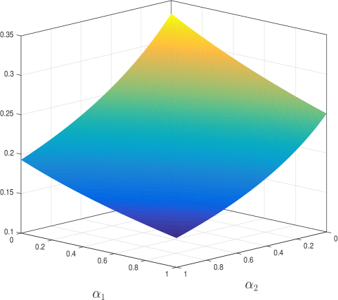
Figure 5: $R$ as a function of $\alpha_{1}\in[0,1]$ and $\alpha_{2}\in[0,1]$ for the MFALK in Example 4.

We note that the analytical results in Proposition 7 agree well with the simulation results obtained using a TASEP model for translation that included alternative initiation along the mRNA and ribosome drop-off [74].

The next section describes an application of the MFALK to a biological process.

IV An application: modeling mRNA translation with ribosome drop off

It is believed that during mRNA translation ribosome movement is unidirectional from the 5’ end to the 3’ end, and that ribosomes do not enter in the middle of the coding regions. However, ribosomes can detach from various sites along the mRNA molecule due for example to collisions between ribosomes. This is known as ribosome drop off.

As mentioned in the introduction, ribosome drop off has been the topic of numerous studies [57, 25, 24, 68, 7, 61, 18, 28, 22, 20, 29]. It was suggested that in some cases ribosome drop off is important for proof reading [69], and also that ribosome stalling/abortion plays a role in translational regulation (e.g. see [56, 74]).

It is clear that ribosome abortion has drawbacks. Indeed, translation is the most energetically consuming process in the cell, and abortion results in truncated, non-functional and possibly deleterious proteins. It is believed that transcripts undergo evolutionary selection to minimize abortion and/or its energetic cost [67, 63, 61, 18, 28, 20]. Nevertheless, there seems to be a certain minimal abortion rate even in non-stressed conditions [57, 29]. This basal value was estimated (see more details below) to be of the order or $10^{-4}-10^{-3}$ abortion events per codon in E. coli. In other words, in every codon one out of $1,000-10,000$ decoding ribosomes aborts. This value is non-negligible. If we consider a drop-off rate of $4*10^{-4}$ per codon along a coding region of $300$ codons (approximately the average coding region length for E. coli) then on average, around $10$ out of every $100$ ribosomes will fail to complete the translation of the mRNA.

To model translation with ribosome drop off, we use the MFALK with $\gamma_{i}=0$ (i.e. no backwards motion) and $\beta_{i}=0$ (i.e. no attachment to internal sites along the chain) for all $i$. Changing the values of the $\alpha_{i}$s allows to model and analyze the effect of ribosome drop off at different sites along the mRNA molecule. We assume that

$$\lambda_{i}>0,\quad\text{for all }i,$$ (26)

as otherwise the chain decouples into two smaller, disconnected chains. Note that (26) implies that the conditions in Proposition 3 hold, so the model is SO on $C^{n}$ w.r.t. the $L_{1}$ norm, and thus admits a unique globally asymptotically stable equilibrium point $e\in\operatorname{{\mathrm{i}nt}}(C^{n})$.

We study the effect of ribosome drop off on the steady-state protein production rate and ribosome density using real biological data. To this end, we considered $10$ S. cerevisiae genes (see Figures 6 and 7) with various mRNA levels (all genes were sorted according to their mRNA levels and $10$ genes were uniformly sampled from the list). Similarly to the approach used in [48], we divided the mRNAs related to these genes to non-overlapping pieces. The first piece includes the first $9$ codons that are related to various stages of initiation [63]. The other pieces include $10$ non-overlapping codons each, except for the last one that includes between $5$ and $15$ codons.

To model the translation dynamics in these mRNAs using MFALK, we model every piece of mRNA as a site. We estimated the elongation rates $\lambda_{i}$ at each site using ribo-seq data for the codon decoding rates [12], normalized so that the median elongation rate of all S. cerevisiae mRNAs becomes $6.4$ codons per second [23]. The site rate is $(\text{site time})^{-1}$, where site time is the sum over the decoding times of all the codons in the piece of mRNA corresponding to this site. These rates thus depend on various factors including availability of tRNA molecules, amino acids, Aminoacyl tRNA synthetase activity and concentration, and local mRNA folding [12, 1, 63].

The initiation rate $\lambda_{0}$ (that corresponds to the first piece) was estimated based on the ribosome density per mRNA levels, as this value is expected to be approximately proportional to the initiation rate when initiation is rate limiting [48, 36]. Again we applied a normalization that brings the median initiation rate of all S. cerevisiae mRNAs to be $0.8$ [9].

We analyzed the effect of uniform ribosome drop off with a rate in the range of $10^{-5}$ to $10^{-3}$ per codon. This corresponds to $\alpha_{1}=\cdots=\alpha_{n}:=\alpha_{c}$, i.e., all the $\alpha_{i}$s are equal, and $\alpha_{c}$ denote their common value. Since we assumed $10$ codons per site, $\alpha_{c}$ values range from $10^{-4}$ to $10^{-2}$ (ten times the rate associated with a single codon). This makes sense as in the MFALK the level of occupancy in a site is related to the probability to see a ribosome in this site.

Let

$$\rho:=\frac{\sum_{i=1}^{n}e_{i}}{n},$$

denote the steady-state mean ribosomal density. Figures 6 and 7 depict $\rho$ and $R$ in our model as a function of $\alpha_{c}\in[10^{-4},10^{-2}]$. In these figures the genes in the legends are sorted according to their expression levels: the gene at the top (YGR192C) has the highest mRNA levels while the gene at the bottom (YER106W) has the lowest levels. It may be seen that as the drop off (detachment) rate $\alpha_{c}$ increases from $10^{-4}$ to $10^{-2}$, $\rho$ decreases by about $30\%$, and $R$ decreases by about $50\%$. This demonstrate the significant ramifications that ribosomal drop off is expected to have on translation and the importance of modeling drop off.

Note also that there is a strong variability in the effect of drop off on the different genes: for mRNAs with higher expression levels (i.e. mRNAs with higher copy number in the cell) the drop off effect is weaker. It is possible that this is related to stronger evolutionary selection for lower drop off rate in genes with higher mRNA levels. Indeed, highly expressed genes “consume” more ribosomes (due to higher mRNA levels), so a given (per-mRNA) drop off rate is expected to be more deleterious to the cell, and a mutation which decreases the drop of rate in such genes has a higher probability of fixation.

Figure 6: Reduction in steady-state mean density $\rho$ in percent as a function of $\alpha_{c}\in[10^{-4},10^{-2}]$ for $10$ S. cerevisiae genes.

Figure 7: Reduction in steady-state output rate (production rate) $R$ in percent as a function of $\alpha_{c}\in[10^{-4},10^{-2}]$ for $10$ S. cerevisiae genes.

V Discussion

In many important processes biological “particles” move along some kind of a one-dimensional “track”. Examples include gene transcription and translation, cellular transport, and more. The flow can be either bidirectional (as in the case of transcription) or unidirectional (as in the case of translation), with the possibility of both attachment and detachment of particles at different sites along the track. For example, motor proteins like kinesin and dynein that move along a certain microtubule may detach and attach to an overlapping microtubule.

To rigorously model and analyze such processes, we introduced a new deterministic mathematical model that can be derived as the dynamic mean-field approximation of ASEP with Langmuir kinetics, called the MFALK. Our main results show that the MFALK is a monotone and contractive dynamical system. This implies that it admits a globally asymptotically unique equilibrium point, and that it entrains to periodic excitations (with a common period $T>0$) in any of its rates, i.e. the densities along the chain, as well as the output rate, converge to unique period solutions with period $T$.

It is important to note that several known models are special cases of the MFALK. These include for example the RFM [48], the model used in [15] for DNA transcription, and the model of phosphorelays in [11].

Topics for further research include the following. In the RFM, it has been shown that the steady-state production rate is related to the maximal eigenvalue of a certain non-negative, symmetric tridiagonal matrix with elements that are functions of the RFM rates, i.e. the $\lambda_{i}$s [44]. This implies that the mapping $(\lambda_{0},\dots,\lambda_{n})\to R$ is strictly concave, and that sensitivity analysis of $R$ is an eigenvalue sensitivity problem [45]. An interesting research topic is whether $R=R(\lambda_{0},\dots,\lambda_{n},\gamma_{0},\dots,\gamma_{n},\alpha_{1},\dots,\alpha_{n},\beta_{1},\dots,\beta_{n})$ in the MFALK can also be described using such a linear-algebraic approach.

The application of the MFALK to model ribosome drop off suggests an interesting direction for further study, namely, how to design genes that minimize the drop off rate.

Another research direction is motivated by the fact that many of the transport phenomena that can be modeled using the MFALK do not take place in isolation. For example, many mRNA molecules are translated in parallel in the cell. Thus, a natural next step is to study networks of interconnected MFALKs. Graph theory can be used to describe the interconnections between the various MFALKs in the network. In this context, ribosome drop off may perhaps increase the total production rate in the entire system, as it allows ribosomes to detach from slow sites, enter the pool of free ribosomes, and then attach to the initiation sites of other, less crowded, mRNA molecules. However, drop off still incurs the biological “cost” associated to the synthesis of a chain of amino-acids that is only a part of the desired protein. The fact that the MFALK is contractive may prove useful in analyzing networks of MFALKs, as there exist interesting results proving the overall contractivity of a network based on contractivity of the subsystems and their couplings (see, e.g. [5, 50]).

Another interesting topic for further research is studying the effect of controlled detachment rates on the formation of traffic jams. Indeed, it is known that kinesin-family motor proteins are more susceptible to dissociation when their pathway is blocked [14, 62].

Appendix: Proofs

We begin by discussing some symmetry properties of the MFALK, as these will be useful in the proofs later on.

Symmetry

The MFALK enjoys two symmetries that will be useful later on. First, let $z_{i}(t):=1-x_{i}(t)$, $i=1,\dots,n$. In other words, $z_{i}(t)$ is the amount of “free space” at site $i$ at time $t$. Then using (II) yields

$$\dot{z}_{1} =\gamma_{0}(1-z_{1})+\lambda_{1}z_{2}(1-z_{1})+\alpha_{1}(1-z_{1})-\gamma_{1}z_{1}(1-z_{2})-\lambda_{0}z_{1}-\beta_{1}z_{1},$$

$$\dot{z}_{2} =\gamma_{1}z_{1}(1-z_{2})+\lambda_{2}z_{3}(1-z_{2})+\alpha_{2}(1-z_{2})-\gamma_{2}z_{2}(1-z_{3})-\lambda_{1}z_{2}(1-z_{1})-\beta_{2}z_{2},$$

$$\vdots$$

$$\dot{z}_{n} =\gamma_{n-1}z_{n-1}(1-z_{n})+\lambda_{n}(1-z_{n})+\alpha_{n}(1-z_{n})-\gamma_{n}z_{n}-\lambda_{n-1}z_{n}(1-z_{n-1})-\beta_{n}z_{n}.$$ (27)

This is just the MFALK (II), but with the parameters permuted as follows: $\lambda_{k}\to\gamma_{k}$, $\gamma_{k}\to\lambda_{k}$, $\beta_{k}\to\alpha_{k}$, and $\alpha_{k}\to\beta_{k}$ for all $k$. The symmetry here follows from the fact that we can replace the roles of the forward and backward flows in the MFALK.

Next, let $y_{i}(t):=1-x_{n+1-i}(t)$, $i=1,\dots,n$. In other words, $y_{i}(t)$ is the amount of “free space” at site $n+1-i$ at time $t$. Then using (II) yields

$$\dot{y}_{1} =\lambda_{n}(1-y_{1})+\gamma_{n-1}y_{2}(1-y_{1})+\alpha_{n}(1-y_{1})-\lambda_{n-1}y_{1}(1-y_{2})-\gamma_{n}y_{1}-\beta_{n}y_{1},$$

$$\dot{y}_{2} =\lambda_{n-1}y_{1}(1-y_{2})+\gamma_{n-2}y_{3}(1-y_{2})+\alpha_{n-1}(1-y_{2})-\lambda_{n-2}y_{2}(1-y_{3})-\gamma_{n-1}y_{2}(1-y_{1})-\beta_{n-1}y_{2},$$

$$\vdots$$

$$\dot{y}_{n} =\lambda_{1}y_{n-1}(1-y_{n})+\gamma_{0}(1-y_{n})+\alpha_{1}(1-y_{n})-\lambda_{0}y_{n}-\gamma_{1}y_{n}(1-y_{n-1})-\beta_{1}y_{n}.$$ (28)

This is just the MFALK (II), but with the parameters permuted as follows: $\lambda_{k}\to\lambda_{n-k}$, $\gamma_{k}\to\gamma_{n-k}$, $\beta_{k}\to\alpha_{n+1-k}$, and $\alpha_{k}\to\beta_{n+1-k}$ for all $k$. Note that (Symmetry) is simply (Symmetry) with the variable renaming $z_{i}\to y_{n+1-i}$, $i=1,\dots,n$.

Both symmetries are reminiscent of the particle-hole symmetry in ASEP [6, 30]: the basic idea is that the progression of a particle from left to right is also the progression of a hole from right to left.

Proof of Proposition 1. If (4) holds then the MFALK satisfies property (BR) in [35], and [35, Lemma 1] implies (6). If (5) holds then (Symmetry) satisfies property (BR) in [35], and this implies (6). ∎

Proof of Proposition 2. Write the MFALK as $\dot{x}=f(x)$. A calculation shows that the Jacobian matrix $J(x):=\frac{\partial f}{\partial x}(x)$ satisfies $J(x)=L(x)+P$, where $L(x)$ is given in (30), and $P$ is the diagonal matrix

$$P=\operatorname{{\mathrm{d}iag}}(-\lambda_{0}-\gamma_{0}-\alpha_{1}-\beta_{1},-\alpha_{2}-\beta_{2},\dots,-\alpha_{n-1}-\beta_{n-1},\lambda_{n}-\gamma_{n}-\alpha_{n}-\beta_{n}).$$ (29)

Note that $L(x)$ is tridiagonal and Metzler (i.e, every off-diagonal entry is non-negative) for any $x\in C^{n}$.

$$L(x)=\begin{bmatrix}-\lambda_{1}(1-x_{2})-\gamma_{1}x_{2}&\lambda_{1}x_{1}+\gamma_{1}(1-x_{1})&\dots&0\\ \lambda_{1}(1-x_{2})+\gamma_{1}x_{2}&-\lambda_{1}x_{1}-\gamma_{1}(1-x_{1})-\lambda_{2}(1-x_{3})-\gamma_{2}x_{3}&\dots&0\\ 0&\lambda_{2}(1-x_{3})+\gamma_{2}x_{3}&\dots&0\\ &&\vdots&\\ 0&0&\dots&0\\ 0&0&\dots&\lambda_{n-1}x_{n-1}+\gamma_{n-1}(1-x_{n-1})\\ 0&0&\dots&-\lambda_{n-1}x_{n-1}-\gamma_{n-1}(1-x_{n-1})\\ \end{bmatrix}$$ (30)

Recall that the matrix measure $\mu_{1}:\mathbb{R}^{n\times n}\to\mathbb{R}$ induced by the $L_{1}$ norm is given by $\mu_{1}(A)=\max\{c_{1}(A),\dots,c_{n}(A)\}$, where $c_{i}(A)$ is the sum of the elements in column $i$ of $A$ with off-diagonal elements taken with absolute value [64]. For the Jacobian $J$ of the MFALK, $\mu_{1}(J(x))=\eta$ for all $x\in C^{n}$. It is well-known (see, e.g., [3]) that this implies (7). ∎

Proof of Proposition 3. For $\zeta\in[0,1/2]$, let

$$C^{n}_{\zeta}:=\{x\in C^{n}:\;\zeta\leq x_{i}\leq 1-\zeta,\;i=1,\dots,n\}.$$

Note that $C^{n}_{0}=C^{n}$, and that $C^{n}_{\zeta}$ is a strict subcube of $C^{n}$ for all $\zeta\in(0,1/2]$. By Proposition 1, for any $\tau>0$ there exists $\zeta=\zeta(\tau)\in(0,1/2)$, with $\zeta(\tau)\to 0$ as $\tau\to 0$, such that

$$x(t+\tau,a)\in C^{n}_{\zeta},\quad\text{for all }t\geq 0\text{ and all }a\in C^{n}.$$ (31)

For any $x\in C^{n}_{\zeta}$ every entry $L_{ij}$ on the sub- and super-diagonal of $L$ in (30) satisfies $L_{ij}\geq\zeta s$, where $s:=\min_{1\leq i\leq n-1}\{\lambda_{i}+\gamma_{i}\}>0$. Combining this with [35, Theorem 4], implies that for any $\zeta\in(0,1/2]$ there exists $\varepsilon=\varepsilon(\zeta)>0$, and a diagonal matrix $D=\operatorname{{\mathrm{d}iag}}(1,q_{1},q_{1}q_{2},\dots,q_{1}q_{2}\dots q_{n-1})$, with $q_{i}=q_{i}(\varepsilon)>0$, such that the MFALK is contractive on $C^{n}_{\zeta}$ w.r.t. the scaled $L_{1}$ norm defined by $|z|_{1,D}:=|Dz|_{1}$. Furthermore, we can choose $\varepsilon$ such that $\varepsilon(\zeta)\to 0$ as $\zeta\to 0$, and $D(\varepsilon)\to I$ as $\varepsilon\to 0$. Now Thm. 1 in [39] implies that the MFALK is contractive after a small overshoot and short transient (SOST). Prop. 4 in [39] implies that for the MFALK SOST is equivalent to SO, and this completes the proof. ∎

Proof of Proposition 4. We begin by recursively defining two sequences. For all integers $i\geq 1$, let

$$u_{i+1} =1+\ell_{1}+\ell_{2}+\dots+\ell_{i},$$

$$\ell_{i+1} =u_{i}+\ell_{1}+\ell_{2}+\dots+\ell_{i-1}.$$ (32)

with initial conditions $u_{0}=u_{1}=1$, and $\ell_{0}=0$, $\ell_{1}=1$. We claim that for $k=0,1,\dots,n-1$ the steady-state density in site $n-k$ is generically the ratio of two polynomials in $R$:

$$e_{n-k}=\frac{p_{k}(R)}{q_{k}(R)},\quad\text{with }\deg(p_{k}(R))=u_{k},\;\deg(q_{k}(R))=\ell_{k}.$$ (33)

We prove this by induction on $k$. By (III-C), $e_{n}=aR+b$, with $a:=(\lambda_{n}+\gamma_{n}+\beta_{n}+\alpha_{n})^{-1}$ and $b:=(\gamma_{n}+\beta_{n})a$, and this proves (33) for $k=0$. Using (III-C) again yields

$$e_{n-1} =\frac{R+\gamma_{n-1}e_{n}}{\lambda_{n-1}(1-e_{n})+\gamma_{n-1}e_{n}}$$

$$=\frac{R+\gamma_{n-1}(aR+b)}{\lambda_{n-1}+(\gamma_{n-1}-\lambda_{n-1})(aR+b)},$$

and this proves (33) for $k=1$. Now assume that there exists $s\geq 2$ such that (33) holds for $k=0,1,\dots,s-1$. By (III-C),

$$e_{n-s} =\frac{R+\gamma_{n-s}e_{n-s+1}-g_{n-s+1}(e_{n-s+1})-g_{n-s+2}(e_{n-s+2})-\dots-g_{n-1}(e_{n-1})}{\lambda_{n-s}(1-e_{n-s+1})+\gamma_{n-s}e_{n-s+1}},$$

and applying (III-C) and the induction hypothesis yields

$$e_{n-s} =\frac{R+\gamma_{n-s}\frac{p_{s-1}}{q_{s-1}}+(\beta_{n-s+1}+\alpha_{n-s+1})\frac{p_{s-1}}{q_{s-1}}+(\beta_{n-s+2}+\alpha_{n-s+2})\frac{p_{s-2}}{q_{s-2}}+\dots+(\beta_{n-1}+\alpha_{n-1})\frac{p_{1}}{q_{1}}+c}{\lambda_{n-s}+(\gamma_{n-s}-\lambda_{n-s})\frac{p_{s-1}}{q_{s-1}}},$$

where $c:=-\beta_{n-s+1}-\dots-\beta_{n-1}$. Multiplying the numerator and the denominator by $q_{1}\dots q_{s-1}$ yields $e_{n-s}={p_{s}}/{q_{s}}$, where

$$\deg(p_{s}) =\max\{1+\deg(q_{1}\dots q_{s-1}),\deg(p_{s-1}q_{1}\dots q_{s-2}),\dots,\deg(p_{1}q_{2}\dots q_{s-1})\},$$

$$\deg(q_{s}) =\max\{\deg(q_{1}\dots q_{s-1}),\deg(p_{s-1}q_{1}\dots q_{s-2})\}.$$

By the induction hypothesis,

$$\deg(p_{s}) =\max\{1+\ell_{1}+\dots+\ell_{s-1},u_{s-1}+\ell_{1}+\dots+\ell_{s-2},\dots,u_{1}+\ell_{2}+\dots+\ell_{s-1}\},$$

$$\deg(q_{s}) =\max\{\ell_{1}+\dots+\ell_{s-1},u_{s-1}+\ell_{1}+\dots+\ell_{s-2}\}.$$ (34)

It is straightforward to prove that (Symmetry) implies that

$$\ell_{i}\leq u_{i}\leq\ell_{i}+1,\quad i=0,1,2,\dots.$$ (35)

Combining this with (Symmetry) yields $\deg(p_{s})=1+\ell_{1}+\dots+\ell_{s-1}$, and $\deg(q_{s})=u_{s-1}+\ell_{1}+\dots+\ell_{s-2}$. Thus, $\deg(p_{s})=u_{s}$ and $\deg(q_{s})=\ell_{s}$, and this completes the inductive proof of (33). In particular, (33) yields

$$e_{1}=\frac{p_{n-1}(R)}{q_{n-1}(R)},$$ (36)

with $\deg(p_{n-1}(R))=u_{n-1},\;\deg(q_{n-1}(R))=\ell_{n-1}$. Substituting this in the last equation of (III-C) yields

$$v\frac{p_{n-1}}{q_{n-1}}=z-R+\sum_{j=2}^{n-1}g_{j}(e_{j}),$$

where $v:=\lambda_{0}+\gamma_{0}+\beta_{1}+\alpha_{1}$, and $z:=\lambda_{0}+\beta_{1}$. Arguing as above shows that this is a polynomial equation of the form $w(R)=0$, with $\deg(w)=1+\ell_{1}+\dots+\ell_{n-1}=u_{n}$. It is straightforward to prove by induction that (Symmetry) implies that

$$u_{k}=1+\left\lfloor\frac{2^{k}}{3}\right\rfloor,\quad\ell_{k}=\frac{2^{k}-(-1)^{k}}{3},$$

(we note in passing that the latter sequence is known as the Jacobsthal sequence [58]), and this completes the proof of Proposition 4. ∎

Proof of Proposition 5. We begin by proving that $R>0$ implies that $\prod_{i=0}^{n}\lambda_{i}>\prod_{i=0}^{n}\gamma_{i}$. If $R>0$ then (18) yields

$$\lambda_{0}(1-e_{1}) >\gamma_{0}e_{1},$$

$$\lambda_{i}e_{i}(1-e_{i+1}) >\gamma_{i}e_{i+1}(1-e_{i}),\quad i=1,\dots,n-1,$$

$$\lambda_{n}e_{n} >\gamma_{n}(1-e_{n}).$$ (37)

Multiplying all these inequalities, and using the fact that $e\in\operatorname{{\mathrm{i}nt}}(C^{n})$ yields

$$\prod_{i=0}^{n}\lambda_{i}>\prod_{i=0}^{n}\gamma_{i}.$$ (38)

To prove the converse implication, assume that (38) holds. Multiplying both sides of this inequality by the strictly positive term $\prod_{j=1}^{n}e_{j}(1-e_{j})$ yields

$$\prod_{i=0}^{n}a_{i}>\prod_{i=0}^{n}b_{i},$$

where $a_{0}:=\lambda_{0}(1-e_{1})$, $a_{i}:=\lambda_{i}e_{i}(1-e_{i+1})$, $i=1,\dots,n-1$, $a_{n}=\lambda_{n}e_{n}$, $b_{0}:=\gamma_{0}e_{1}$, $b_{i}:=\gamma_{i}e_{i+1}(1-e_{i})$, $i=1,\dots,n-1$, and $b_{n}=\gamma_{n}(1-e_{n})$. This means that $a_{\ell}>b_{\ell}$ for some index $\ell\in\{0,\dots,n\}$. Since $R=a_{\ell}-b_{\ell}$ (see (18)), it follows that $R>0$. Summarizing, we showed that $R>0$ if and only if $\prod_{i=0}^{n}\lambda_{i}>\prod_{i=0}^{n}\gamma_{i}$. The proof that $R<0$ if and only if $\prod_{i=0}^{n}\lambda_{i}<\prod_{i=0}^{n}\gamma_{i}$ is similar. This implies that $R=0$ if and only if $\prod_{i=0}^{n}\lambda_{i}=\prod_{i=0}^{n}\gamma_{i}$. This completes the proof of (19).

To prove (20), note that (18) yields

$$e_{n} =\frac{R+\gamma_{n}}{\lambda_{n}+\gamma_{n}},$$

$$e_{i} =\frac{R+\gamma_{i}e_{i+1}}{\lambda_{i}(1-e_{i+1})+\gamma_{i}e_{i+1}},\quad i=n-1,\dots,1,$$

$$e_{1} =\frac{\lambda_{0}-R}{\lambda_{0}+\gamma_{0}}.$$ (39)

Substituting $R=0$ completes the proof of Prop. 5. ∎

Proof of Proposition 6. Since the Jacobian $J(x)$ of the MFALK is Metzler (i.e, every off-diagonal entry is non-negative) for any $x\in C^{n}$, the MFALK is a cooperative system [60], and this yields (24).

When $\lambda_{i}+\gamma_{i}>0$, $i=1,\dots,n-1$, the matrix $L(x)$ and, therefore, $J(x)$, is irreducible for every $x\in\operatorname{{\mathrm{i}nt}}(C^{n})$, and combining this with Proposition 1 implies (25) (see, e.g., [60, Ch. 4]). ∎

Proof of Theorem 1. The Jacobian of the PMFALK is $J(t,x(t))=L(t,x(t))+P(t)$, with $L$ given in (30), and $P$ is given in (29) (but now with time-varying rates). Pick an initial time $t_{0}\geq 0$, and $\tau_{0}>0$. The stated conditions guarantee the existence of $\zeta\in(0,1/2)$ such that $x(t,t_{0},a)\in C^{n}_{\zeta}$ for all $t\geq t_{0}+\tau$ and all $a\in C^{n}$. Also, [35, Thm. 4] implies that there exists a diagonally-scaled $L_{1}$ norm such that the PMFALK is contractive on $C^{n}_{\zeta}$ w.r.t. this norm. Now entrainment follows from known results on contractive systems with a periodic excitation (see, e.g. [49]). ∎

Proof of Proposition 7. First, using Remark 1 and the argument used in the proof of [46, Prop. 4] shows that all the derivatives in the statement of of Proposition 7 exist.

Given a MFALK, pick $j\in\{1,\dots,n\}$ and consider the new MFALK obtained by changing $\alpha_{j}$ to $\tilde{\alpha}_{j}$, with $\tilde{\alpha}_{j}>\alpha_{j}$, and all other rates unchanged. Let $\tilde{e}$, $\tilde{R}$ denote the steady-state density and production rate in the modified MFALK. Seeking a contradiction, assume that

$$\tilde{e}_{n}\geq e_{n}.$$ (40)

Then (14) implies that

$$\tilde{R}\geq R,$$ (41)

and if $j=n$ then $\tilde{R}>R$. By (III-C) with $i=n-1$, $R=\lambda_{n-1}e_{n-1}(1-e_{n})-\gamma_{n-1}e_{n}(1-e_{n-1})$ and $\tilde{R}=\lambda_{n-1}\tilde{e}_{n-1}(1-\tilde{e}_{n})-\gamma_{n-1}\tilde{e}_{n}(1-\tilde{e}_{n-1})$, and combining this with (40) and (41) yields

$$\tilde{e}_{n-1}\geq e_{n-1}.$$ (42)

Now using (III-C) with $i=n-2$ yields $\tilde{e}_{n-2}\geq e_{n-2}$, and $\tilde{e}_{n-2}>e_{n-2}$ if $j=n-1$. Proceeding in this way shows that

$$\tilde{e}_{k} \geq e_{k},\quad k=n,n-1,\dots,j,$$ (43)

$$\tilde{e}_{k} >e_{k},\quad k=j-1,j-2,\dots,1.$$ (44)

Combining this with (III-C) with $i=0$ yields $\tilde{R}<R$. This contradicts (41), so

$$\tilde{e}_{n}>e_{n}.$$ (45)

Proceeding as above yields $\tilde{e}_{i}>e_{i}$ for all $i$, so $\frac{\partial e_{i}}{\partial\alpha_{j}}<0$ for all $i,j$. The proofs of all the other equations in Prop. 7 are very similar and therefore omitted. ∎

References

- [1] B. Alberts, A. Johnson, J. Lewis, M. Raff, K. Roberts, and P. Walter, Molecular Biology of the Cell. New York: Garland Science, 2008.
- [2] R. J. R. Algar, T. Ellis, and G. Stan, “Modelling essential interactions between synthetic genes and their chassis cell,” in Proc. 53rd IEEE Conference Decision and Control, LA, 2014, pp. 5437–5444.
- [3] Z. Aminzare and E. D. Sontag, “Contraction methods for nonlinear systems: A brief introduction and some open problems,” in Proc. 53rd IEEE Conf. on Decision and Control, Los Angeles, CA, 2014, pp. 3835–3847.
- [4] Y. Arava, Y. Wang, J. D. Storey, C. L. Liu, P. O. Brown, and D. Herschlag, “Genome-wide analysis of mRNA translation profiles in Saccharomyces cerevisiae,” Proceedings of the National Academy of Sciences, vol. 100, no. 7, pp. 3889–3894, 2003.
- [5] M. Arcak, “Certifying spatially uniform behavior in reaction-diffusion PDE and compartmental ODE systems,” Automatica, vol. 47, no. 6, pp. 1219–1229, 2011.
- [6] R. A. Blythe and M. R. Evans, “Nonequilibrium steady states of matrix-product form: a solver’s guide,” J. Phys. A: Math. Gen., vol. 40, no. 46, pp. R333–R441, 2007.
- [7] Y. Chadani, K. Ono, S. Ozawa, Y. Takahashy, K. Takay, H. Nanamiya, Y. Tozawa, K. Kutsukake, and T. Abo, “Ribosome rescue by Escherichia coli arf-a (yhdl) in the absence of trans-translation systems,” Mol. Microbiol., vol. 78, pp. 796–808, 2010.
- [8] A. C. M. Cheung and P. Cramer, “Structural basis of RNA polymerase II backtracking, arrest and reactivation,” Nature, vol. 471, no. 7337, pp. 249–253, 03 2011.
- [9] D. Chu, E. Kazana, N. Bellanger, T. Singh, M. F. Tuite, and T. von der Haar, “Translation elongation can control translation initiation on eukaryotic mRNAs,” EMBO J., vol. 33, no. 1, pp. 21–34, 2014.
- [10] L. S. Churchman and J. S. Weissman, “Nascent transcript sequencing visualizes transcription at nucleotide resolution,” Nature, vol. 469, no. 7330, pp. 368–373, 01 2011.
- [11] A. Csikasz-Nagy, L. Cardelli, and O. S. Soyer, “Response dynamics of phosphorelays suggest their potential utility in cell signaling,” J. Royal Society Interface, vol. 8, pp. 480–488, 2011.
- [12] A. Dana and T. Tuller, “Mean of the typical decoding rates: a new translation efficiency index based on the analysis of ribosome profiling data,” G3, vol. 5, no. 1, pp. 73–80, 2014.
- [13] C. Desoer and H. Haneda, “The measure of a matrix as a tool to analyze computer algorithms for circuit analysis,” IEEE Trans. Circuit Theory, vol. 19, pp. 480–486, 1972.
- [14] R. Dixit, J. L. Ross, Y. E. Goldman, and E. L. Holzbaur, “Differential regulation of dynein and kinesin motor proteins by tau,” Science, vol. 319, pp. 1086–1089, 2008.
- [15] S. Edri, E. Gazit, E. Cohen, and T. Tuller, “The RNA polymerase flow model of gene transcription,” IEEE Trans. Biomedical Circuits and Systems, vol. 8, no. 1, pp. 54–64, 2014.
- [16] T. Ezaki and K. Nishinari, “Exact stationary distribution of an asymmetric simple exclusion process with Langmuir kinetics and memory reservoirs,” Journal of Physics A: Mathematical and Theoretical, vol. 45, no. 18, p. 185002, 2012.
- [17] M. J. García-Meseguer, J. A. V. de Labra, M. Garcia-Moreno, F. García-Canovas, B. H. Havsteen, and R. Varon, “Mean residence times in linear compartmental systems. Symbolic formulae for their direct evaluation,” Bull. Math. Biol., vol. 65, pp. 279–308, 2003.
- [18] M. A. Gilchrist and A. Wagner, “A model of protein translation including codon bias, nonsense errors, and ribosome recycling,” J. Theoretical Biology, vol. 239, no. 4, pp. 417–34, 2006.
- [19] F. S. Heldt, C. A. Brackley, C. Grebogi, and M. Thiel, “Community control in cellular protein production: consequences for amino acid starvation,” Philosophical Trans. Royal Society of London A: Mathematical, Physical and Engineering Sciences, vol. 373, no. 2056, 2015.
- [20] S. D. Hooper and O. Berg, “Gradients in nucleotide and codon usage along Escherichia coli genes,” Nucleic Acids Res, vol. 28, pp. 3517–3523, 2000.
- [21] J. A. Jacquez and C. P. Simon, “Qualitative theory of compartmental systems,” SIAM Review, vol. 35, no. 1, pp. 43–79, 1993.
- [22] F. Jorgensen and C. Kurland, “Processivity errors of gene expression in Escherichia coli,” J. Mol. Biol., vol. 215, pp. 511–521, 1990.
- [23] T. V. Karpinets, D. J. Greenwood, C. E. Sams, and J. T. Ammons, “RNA: protein ratio of the unicellular organism as a characteristic of phosphorous and nitrogen stoichiometry and of the cellular requirement of ribosomes for protein synthesis,” BMC Biol., vol. 4, no. 30, pp. 274–80, 2006.
- [24] K. Keiler, “Mechanisms of ribosome rescue in bacteria,” Nat. Rev. Microbiol., vol. 13, pp. 285–297, 2015.
- [25] K. Keiler, P. Waller, and R. Sauer, “Role of a peptide tagging system in degradation of proteins synthesised from damaged messenger rna,” Science, vol. 271, pp. 990–993, 1996.
- [26] B. S. Kerner, “The physics of green-wave breakdown in a city,” Europhysics Letters, vol. 102, no. 2, p. 28010, 2013.
- [27] S. Klumpp and T. Hwa, “Traffic patrol in the transcription of ribosomal RNA,” RNA Biol., vol. 6, no. 4, pp. 392–4, 2009.
- [28] C. Kurland, “Translational accuracy and the fitness of bacteria,” Ann. Rev. Genet., vol. 26, pp. 29–50, 1992.
- [29] C. Kurland and R. Mikkola, Starvation in Bacteria. NY: Plenum Press, 1993, ch. The impact of nutritional state on the microevolution of ribosomes, pp. 225–238.
- [30] G. Lakatos, T. Chou, and A. Kolomeisky, “Steady-state properties of a totally asymmetric exclusion process with periodic structure,” Phys. Rev. E, vol. 71, p. 011103, 2005.
- [31] C. Leduc, K. Padberg-Gehle, V. Varga, D. Helbing, S. Diez, and J. Howard, “Molecular crowding creates traffic jams of kinesin motors on microtubules,” Proceedings of the National Academy of Sciences, vol. 109, pp. 6100–6105, 2012.
- [32] R. Lipowsky and S. Klumpp, “Life is motion: multiscale motility of molecular motors,” Physica A: Statistical Mechanics and its Applications, vol. 352, no. 1, pp. 53–112, 2005.
- [33] R. Lipowsky, S. Klumpp, and T. M. Nieuwenhuizen, “Random walks of cytoskeletal motors in open and closed compartments,” Phys. Rev. Lett., vol. 87, no. 10, p. 108101, 2001.
- [34] W. Lohmiller and J.-J. E. Slotine, “On contraction analysis for non-linear systems,” Automatica, vol. 34, pp. 683–696, 1998.
- [35] M. Margaliot, E. D. Sontag, and T. Tuller, “Entrainment to periodic initiation and transition rates in a computational model for gene translation,” PLoS ONE, vol. 9, no. 5, p. e96039, 2014.
- [36] M. Margaliot and T. Tuller, “On the steady-state distribution in the homogeneous ribosome flow model,” IEEE/ACM Trans. Computational Biology and Bioinformatics, vol. 9, pp. 1724–1736, 2012.
- [37] M. Margaliot and T. Tuller, “Stability analysis of the ribosome flow model,” IEEE/ACM Trans. Computational Biology and Bioinformatics, vol. 9, pp. 1545–1552, 2012.
- [38] M. Margaliot and T. Tuller, “Ribosome flow model with positive feedback,” J. Royal Society Interface, vol. 10, p. 20130267, 2013.
- [39] M. Margaliot, E. D. Sontag, and T. Tuller, “Contraction after small transients,” Automatica, vol. 67, pp. 178–184, 2016.
- [40] J. Mierczynski, “A class of strongly cooperative systems without compactness,” Colloq. Math., vol. 62, pp. 43–47, 1991.
- [41] E. Nudler, “RNA polymerase backtracking in gene regulation and genome instability,” Cell, vol. 149, no. 7, pp. 1438–1445, 2015.
- [42] A. Parmeggiani, T. Franosch, and E. Frey, “Phase coexistence in driven one-dimensional transport,” Phys. Rev. Lett., vol. 90, p. 086601, 2003.
- [43] A. Parmeggiani, T. Franosch, and E. Frey, “Totally asymmetric simple exclusion process with Langmuir kinetics,” Phys. Rev. E, vol. 70, p. 046101, 2004.
- [44] G. Poker, Y. Zarai, M. Margaliot, and T. Tuller, “Maximizing protein translation rate in the nonhomogeneous ribosome flow model: a convex optimization approach,” J. Royal Society Interface, vol. 11, no. 100, 2014.
- [45] G. Poker, M. Margaliot, and T. Tuller, “Sensitivity of mRNA translation,” Sci. Rep., vol. 5, p. 12795, 2015.
- [46] A. Raveh, M. Margaliot, E. D. Sontag, and T. Tuller, “A model for competition for ribosomes in the cell,” J. Royal Society Interface, vol. 116, no. 20151062, 2016.
- [47] A. Raveh, Y. Zarai, M. Margaliot, and T. Tuller, “Ribosome flow model on a ring,” IEEE/ACM Trans. Computational Biology and Bioinformatics, vol. 12, no. 6, pp. 1429–1439, 2015.
- [48] S. Reuveni, I. Meilijson, M. Kupiec, E. Ruppin, and T. Tuller, “Genome-scale analysis of translation elongation with a ribosome flow model,” PLOS Computational Biology, vol. 7, p. e1002127, 2011.
- [49] G. Russo, M. di Bernardo, and E. D. Sontag, “Global entrainment of transcriptional systems to periodic inputs,” PLOS Computational Biology, vol. 6, p. e1000739, 2010.
- [50] G. Russo, M. di Bernardo, and E. D. Sontag, “A contraction approach to the hierarchical analysis and design of networked systems,” IEEE Trans. Automat. Control, vol. 58, no. 5, pp. 1328–1331, 2013.
- [51] I. W. Sandberg, “On the mathematical foundations of compartmental analysis in biology, medicine, and ecology,” IEEE Trans. Circuits and Systems, vol. 25, no. 5, pp. 273–279, 1978.
- [52] A. Schadschneider, D. Chowdhury, and K. Nishinari, Stochastic Transport in Complex Systems: From Molecules to Vehicles. Elsevier, 2011.
- [53] M. Schliwa and G. Woehlke, “Molecular motors,” Nature, vol. 422, pp. 759–765, 2003.
- [54] J. W. Shaevitz, E. A. Abbondanzieri, R. Landick, and S. M. Block, “Backtracking by single RNA polymerase molecules observed at near-base-pair resolution,” Nature, vol. 426, no. 6967, pp. 684–687, 12 2003.
- [55] L. B. Shaw, R. K. P. Zia, and K. H. Lee, “Totally asymmetric exclusion process with extended objects: a model for protein synthesis,” Phys. Rev. E, vol. 68, p. 021910, 2003.
- [56] C. Shoemaker, D. Eyler, and R. Green, “Dom34:hbs1 promotes subunit dissociation and peptidyl-tRNA drop-off to initiate no-go decay,” Science, vol. 330, no. 6002, pp. 369–72, 2010.
- [57] C. Sin, D. Chiarugi, and A. Valleriani, “Quantitative assessment of ribosome drop-off in E. coli,” Nucleic Acids Res., vol. 44, no. 6, pp. 2528–37, 2016.
- [58] N. J. A. Sloane and S. Plouffe, The Encyclopedia of Integer Sequences. Academic Press, 1995.
- [59] J. Smillie, “Competitive and cooperative tridiagonal systems of differential equations,” SIAM J. Mathematical Analysis, vol. 15, pp. 530–534, 1984.
- [60] H. L. Smith, Monotone Dynamical Systems: An Introduction to the Theory of Competitive and Cooperative Systems, ser. Mathematical Surveys and Monographs. Providence, RI: Amer. Math. Soc., 1995, vol. 41.
- [61] A. Subramaniam, B. Zid, and E. O’Shea, “An integrated approach reveals regulatory controls on bacterial translation elongation,” Cell, vol. 159, no. 5, pp. 1200–11, 2014.
- [62] I. A. Telley, P. Bieling, and T. Surrey, “Obstacles on the microtubule reduce the processivity of kinesin-1 in a minimal in vitro system and in cell extract,” Biophys. J., vol. 96, pp. 3341–3353, 2009.
- [63] T. Tuller and H. Zur, “Multiple roles of the coding sequence 5’ end in gene expression regulation,” Nucleic Acids Res., vol. 43, no. 1, pp. 13–28, 2015.
- [64] M. Vidyasagar, Nonlinear Systems Analysis. Englewood Cliffs, NJ: Prentice Hall, 1978.
- [65] R. Willmann, G. Schütz, and D. Challet, “Exact Hurst exponent and crossover behavior in a limit order market model,” Physica A: Statistical Mechanics and its Applications, vol. 316, no. 1, pp. 430–440, 2002.
- [66] A. Yonath, “Ribosomes: Ribozymes that survived evolution pressures but is paralyzed by tiny antibiotics,” in Macromolecular Crystallography: Deciphering the Structure, Function and Dynamics of Biological Molecules, A. M. Carrondo and P. Spadon, Eds. Dordrecht: Springer Netherlands, 2012, pp. 195–208.
- [67] Z. Zafrir, H. Zur, and T. Tuller, “Selection for reduced translation costs at the intronic 5’ end in fungi,” DNA Res., vol. 23, no. 4, pp. 377–94, 2016.
- [68] H. Zaher and R. Green, “A primary role for elastase factor 3 in quality control during translation elongation in Escherichia coli,” Cell, vol. 147, pp. 396–408, 2011.
- [69] S. Zaher and R. Green, “Quality control by the ribosome following peptide bond formation,” Nature, vol. 457, pp. 161–166, 2009.
- [70] Y. Zarai, M. Margaliot, E. D. Sontag, and T. Tuller, “Controlling mRNA translation,” 2016, submitted.
- [71] Y. Zarai, M. Margaliot, and T. Tuller, “Explicit expression for the steady-state translation rate in the infinite-dimensional homogeneous ribosome flow model,” IEEE/ACM Trans. Computational Biology and Bioinformatics, vol. 10, pp. 1322–1328, 2013.
- [72] G. Zhang, I. Fedyunin, O. Miekley, A. Valleriani, A. Moura, and Z. Ignatova, “Global and local depletion of ternary complex limits translational elongation,” Nucleic Acids Res., vol. 38, no. 14, pp. 4778–4787, 2010.
- [73] R. K. P. Zia, J. Dong, and B. Schmittmann, “Modeling translation in protein synthesis with TASEP: A tutorial and recent developments,” J. Statistical Physics, vol. 144, pp. 405–428, 2011.
- [74] A. Zupanic, C. Meplan, S. M. Grellscheid, J. C. Mathers, T. B. Kirkwood, J. E. Hesketh, and D. P. Shanley, “Detecting translational regulation by change point analysis of ribosome profiling data sets,” RNA, vol. 20, no. 10, pp. 1507–1518, 2014.