Lower bound for sensitivity of graph properties

Abstract

We prove that the sensitivity of any non-trivial graph property on $n$ vertices is at least $\lfloor\frac{1}{2}n\rfloor$ , provided $n$ is sufficiently large.

1 Introduction

The notion of the sensitivity complexity of a boolean function (see definition in section $2$), or just sensitivity, has been widely studied, since introduced by Cook and Dwork in [4], where it was used to derive tight lower bounds for the running time of a PRAM computing boolean function $f$. Simon [12] proved that if all of $f$’s coordinates have positive influence, one has the lower bound of $s(f)=\Omega(\log{n})$. This bound is known to be asymptotically tight, as demonstrated by the so called monotone address function.

There have been attempts to find lower bounds for the sensitivity of certain classes of boolean functions. In particular, the class of weakly symmetric functions has been studied. For this class, the best known lower bound is $s(f)=\Omega(\log{n})$ for any non-constant weakly symmetric function $f$ in $n$ variables. Indeed, for weakly symmetric functions all coordinates have the same influence, from which it follows that all coordinates have positive influences if $f$ is also non-constant, and as we have already mentioned, this guarantees $s(f)=\Omega(\log{n})$.

Yet, so far, every non-constant weakly symmetric function $f$ found, has sensitivity $s(f)=\Omega(n^{1/3})$. Turan conjectured in [15] that there exists some absolute constant $c>0$, so that $s(f)=\Omega(n^{c})$ for any non-constant weakly symmetric boolean function.

Perhaps the main open problem regarding sensitivity, is its relation to the seemingly similar notion of block sensitivity (see section $2$ for definition). Nisan and Szegedy posed the conjecture [10] in $1994$ that the two are polynomially equivalent.

This would have important implications, since block sensitivity is known to be polynomially equivalent to many important measures of the complexity of a function, including Decision tree complexity, certificate complexity, degree as a real polynomial, Quantum query complexity etc. Finding bounds on the separations between pairs of the aforementioned measures is a lively field (see, for example, [1, 2, 9, 10]). While at the moment block sensitivity can only be shown to be exponentially upper bounded by sensitivity [8], the largest known gap is quadratic, as shown first by [11]. For an excellent survey on the sensitivity conjecture, see [6].

The sensitivity conjecture implies Turan’s conjecture on weakly symmetric functions, because if $f$ is weakly symmetric, then $bs(f)=\Omega(n^{\frac{1}{3}})$ [14].

Turan, in the same paper [15], studied the sensitivity of graph properties. He showed that for any non-trivial graph property $f$ for $n$ vertices (and so, ${n\choose 2}$ boolean variables), $s(f)\geq\lfloor\frac{n}{4}\rfloor$. He conjectured:

Conjecture 1.

[15] Let $f$ be a non-trivial graph property for graphs with $n$ vertices. Then $s(f)\geq n-1$.

Turan’s conjecture is the best possible, since the property ”$G$ has a vertex of degree $n-1$” has sensitivity $n-1$. Wegener [16] proved $s(f)\geq n-1$ for any non-trivial monotone graph property $f$, but made no improvement on Turan’s lower bound for graph properties in general. This was done only in $2011$, when Sun [13] improved Turan’s lower bound to $s(f)\geq\frac{6}{17}n$. In [5], lower bounds for the sensitivity of bipartite graph-properties were obtained.

Our main result in this paper, is an improvemnt of the lower bound in [13]. We prove:

Theorem 1.

Let $f$ be a non-trivial graph property on $n$ vertices, for sufficiently large $n$. Then $s(f)\geq\lfloor\frac{1}{2}n\rfloor$.

The paper is organized as follows: in section $2$, we provide the relevant definitions and notations. The reader familiar with the topic may want to skip to subsection $2.2$, where we provide non-standard definitions used in this paper. In section $3$, we prove Theorem 1, and in section $4$ we discuss related open problems.

2 Preliminaries and Definitions

2.1 Standard Definitions

Definition 2.1.

Let $f:\{0,1\}^{n}\to\{0,1\}$ be a boolean function, and $x\in\{0,1\}^{n}$ some point. The sensitivity of $f$ at point $x$, which we denote as $s(f,x)$, is

$$s(f,x):=|\{i\in[n]|f(x\oplus e_{i})\neq f(x)\}|.$$

In other words, it is the number of neighbours $y$ of $x$ in the hamming cube, with $f(y)\neq f(x)$.

The sensitivity of f, $s(f)$, is just the maximum sensitivity over all points:

$$s(f)=\max_{x}s(f,x).$$

Definition 2.2.

Let $f:\{0,1\}^{n}\to\{0,1\}$ be a boolean function, and $x\in\{0,1\}^{n}$ some point. The block sensitivity of $f$ at point $x$, which we denote as $bs(f,x)$, is the maximum number $t$, such that there are $t$ pairwise disjoint subsets of $[n]$, $B_{1},\dots,B_{t}$, with the property $f(x)\neq f(x^{B_{i}})$ for all $i\in[t]$. Here, $x^{B_{i}}$ is obtained by flipping in $x$ every coordinate $j\in B_{i}$.

The block sensitivity of f, $bs(f)$, is just the maximum block sensitivity over all points:

$$bs(f)=\max_{x}bs(f,x).$$

Of course $s(f)\leq bs(f)$ for every boolean function $f$, because each block can be a sensitive coordinate.

Definition 2.3.

A group $\Gamma\leq S_{n}$ is called transitive, if for every $i,j\in[n]$, there exists an element $\pi\in\Gamma$, so that $\pi(i)=j$.

Definition 2.4.

Let $x=x_{1}\dots x_{n}$ be an $n$ bit boolean string, and let $\pi\in S_{n}$ be some permutation of $n$ elements. Then the action of $\pi$ on $x$, which we denote by $\pi x$, is the string $\pi x:=x_{\pi(1)}\dots x_{\pi(n)}$.

Definition 2.5.

A boolean function $f:\{0,1\}^{n}\to\{0,1\}$ is called weakly symmetric, if there is some transitive group $\Gamma\leq S_{n}$, so that for every $x\in\{0,1\}^{n}$ and every $\pi\in\Gamma$, $f(x)=f(\pi x)$. We say, in that case, that $f$ is closed under $\Gamma$.

We now move on to discuss graph properties.

For every $\{i,j\}\in{[n]\choose 2}$, define a suitable boolean variable $x_{\{i,j\}}\in\{0,1\}$. A string $x\in\{0,1\}^{n\choose 2}$, then, can be considered simply as an assignment to all these variables. This set can also be identified with the set of all graphs with vertex set $[n]$, via the bijection

$$x\longrightarrow\Big{(}[n],\big{\{}\{i,j\}\in{[n]\choose 2}\big{|}x_{i,j}=1\big{\}}\Big{)}.$$ (1)

Consider the group $S_{n}$ acting on the set ${[n]\choose 2}$ in the following way: for $\{i,j\}\in{[n]\choose 2}$, and $\pi\in S_{n}$, we write $\pi\{i,j\}:=\{\pi(i),\pi(j)\}$. Note that $S_{n}$ acts transitively on ${[n]\choose 2}$.

Definition 2.6.

$f:\{0,1\}^{[n]\choose 2}\to\{0,1\}$ is called a graph property, if for every $\pi\in S_{n}$ and every point $x\in\{0,1\}^{[n]\choose 2}$, $f(x)=f(\pi x)$.

By abuse of notation, from now on we shall think of the domain of $f$ as the family of all graphs with vertex set $[n]$, using the bijection in (1). $f$ being a graph property, in this notation, means that $f(G)=f(H)$ whenever $G$ and $H$ are isomorphic graphs. Furthermore, we will sometimes think of a graph simply as its set of edges, so for example $|G|$ will denote the number of edges in $G$. This should not create confusion, since the vertex set is always understood to be $[n]$, unless explicitly stated otherwise.

2.2 non-standard Definitions and notations

Throughout this subsection, $f$ is a non-trivial graph property on graphs with vertex set $[n]$, and $f(\overline{K_{n}})=0$.

Definition 2.7.

For a graph $G=([n],E)$, $G\neq\overline{K_{n}}$, we define the positive minimum degree of $G$, denoted by $\delta^{\prime}(G)$, to be the minimum degree of any non-isolated vertex in $G$. We write $\delta^{\prime}(\overline{K_{n}})=\infty$.
For any natural number $k$, we denote by $G_{[k]}$ the maximal subgraph of $G$ (with vertex set $[n]$), for which $\delta^{\prime}(G_{[k]})\geq k$.

Observe that if $\delta^{\prime}(G)\geq k$, then $G_{[k]}=G$. Otherwise $G_{[k]}\subsetneq G$.

Definition 2.8.

Any graph $G$ can have three kinds of connected components: isolated vertices, components containing a cycle, and trees containing at least one edge. We define the positive minimum tree component size, which we denote by $c(G)$, to be the number of edges in the smallest connected component of $G$ that is a tree, but not an isolated vertex. If $G$ has no connected components of this form, we write $c(G)=\infty$.

For any natural number $k$, we denote by $G_{(k)}$ the maximal subgraph of $G$ (with vertex set $[n]$), so that $c(G_{(k)})\geq k$.
Observe that if $c(G)\geq k$, then $G_{(k)}=G$. Otherwise $G_{(k)}\subsetneq G$.

Definition 2.9.

We call a graph $G$ minimal with respect to $f$, if $f(G)=1$ and $f(G^{\prime})=0$ for every graph $G^{\prime}\subsetneq G$. The set of all minimal graphs for $f$ is denoted by $m(f)$. Notice that $m(f)\neq\emptyset$ because we took $f$ to be non-trivial.

We write $\delta^{\prime}(f)=\min_{G\in m(f)}\delta^{\prime}(G)$, and $c(f)=\min_{G\in m(f)}c(G)$.

Definition 2.10.

Let $T$ be a tree with $k$ edges. A tree construction sequence of $T$, is a sequence of $k$ trees $T^{(1)},\dots,T^{(k)}$ such that:

• For every $i\in[k]$, $T^{(i)}$ is a tree with $i$ edges.

• $T^{(k)}$ is isomorphic to $T$.

• For every $i\in[k-1]$, $T^{(i+1)}$ is obtained from $T^{(i)}$ by adding a new vertex, and connecting this vertex by an edge to some other vertex in $T^{(i)}$.

(See Figure 1).

Figure 1: Tree construction sequence

3 proof of main theorem

Before proving the main theorem, we need the following lemma, found in [13]

Lemma 3.1.

Let $f$ be a graph property, and $G$ be a graph. Let $v\in V(G)$ be a vertex of degree one, and $e=\{v,u\}$ the unique edge in $G$ where $v$ occurs. Then either $s(f)\geq|I(G)|+1$, or $f(G)=f(G\setminus e)$.

Proof.

Let $f,G,v,e$ be as in the statement of the lemma. Assume that $f(G)\neq f(G\setminus e)$, and let $I(G)=\{w_{1},\dots,w_{|I(G)|}\}$ . Observe that $G$ is isomorphic to $(G\setminus e)\cup\{u,w_{i}\}$ for every $1\leq i\leq|I(G)|$. Thus, $f(G)=f((G\setminus e)\cup\{u,w_{i}\})$ for every $w_{i}\in I(G)$. But this means that $f(G\setminus e)\neq f((G\setminus e)\cup\{u,w_{i}\})$, and as mentioned, $f(G\setminus e)\neq f(G)$. So the sensitivity of $f$ at $G\setminus e$ is at least $|I(G)|+1$, as claimed. ∎

proof of Theorem 1.

Throughout the proof, we assume that all graphs have vertex set $[n]$. Assume without loss of generality that for the graph with no edges $\overline{K_{n}}$, $f(\overline{K_{n}})=0$, and assume by contradiction that $s(f)<\lfloor\frac{n}{2}\rfloor$.

It is an easy, but important, observation, that if $G\in m(f)$ then $G$ is sensitive at any of the edges it contains, which means that

$$|G|\leq s(f,G)<\lfloor\frac{1}{2}n\rfloor$$ (2)

As already mentioned, by our assumptions on $f$, $c(f)$ and $\delta^{\prime}(f)$ are well defined. We divide our proof to three cases, based on their possible values:

Case 1 ($\delta^{\prime}(f)\geq 2$)

Let $G\in m(f)$, $\delta^{\prime}(G)=\delta^{\prime}(f)$. In this case, since there are no vertices of degree one in $G$, in particular any connected component which is not an isolated vertex, can not be a tree. Thus, for every connected component in $G$, the number of edges in that component is at least the number of vertices in it. Summing over all connected components, produces the inequality

$$|G|+|I(G)|\geq n.$$ (3)

Combining this with (2)

$$|I(G)|>\frac{1}{2}n$$ (4)

We show an algorithm that finds a graph $G^{\prime}\subsetneq G$, with $f(G^{\prime})=1$. But we took $G\in m(f)$, which is a contradiction. Denote the isolated vertices of $G$ by $I(G)=\{v_{1},\dots,v_{m}\}$.

Algorithm 1 Algorithm for $\delta^{\prime}(f)\geq 2$

  $H\leftarrow G$

  $k\leftarrow\delta^{\prime}(G)$

  $m\leftarrow|I(G)|$

  Find a vertex $v$ of degree $k$. Denote $N(v)=\{u,u_{1},\dots,u_{k-1}\}$

  for $i:=1$ to $k-1$ do

     for $j:=1$ to $m$ do

        if $\exists e\in G$ so that $f(H\setminus e)=f(H)$ then

           $H\leftarrow H\setminus e$

           return  some minimal graph $G^{\prime}\subset H$ {We prove that such $G^{\prime}$ must exist}

        end if

        $H\leftarrow H\cup\{u_{i},v_{j}\}$

     end for

  end for

  $H\leftarrow H\setminus\{v,u\}$

  return  some minimal graph $G^{\prime}\subset H$ { We prove that such $G^{\prime}$ must exist}

Claim 1.

At any stage in the algorithm, $f(H)=1$. Thus $f(G^{\prime})=1$.

Proof.

Assume by contradiction that this is not the case. Then there must be a first time during the execution of the algorithm when the value of $f(H)$ becomes zero. When we refer to $H$ in the proof, henceforth, we mean the graph $H$ in the algorithm immediately after its value becomes zero for the first time. This can occur either during some iteration of the for-loop, or at the end of the loop, while removing edge $\{v,u\}$.

We deal with the latter case first: Let $H^{+}=H\cup\{v,u\}$. That is, the graph in the algorithm just before removing edge $\{v,u\}$. By our assumption $f(H^{+})=1$. But notice that $H\cup\{v_{i},u\}$ is isomorphic to $H^{+}$, for all $1\leq i\leq m$. Thus, $H$ is sensitive at all these edges, and at $\{v,u\}$, which means that
$s(f,H)\geq m+1>\frac{1}{2}n$ , contradicting (4) (see Figure  2(a)).

Next, we deal with the case that the value of $f(H)$ becomes zero for the first time during some iteration of the for-loop. This can not happen inside the if-condition, because the algorithm only removes edge $e$ inside the if-condition if guaranteed that removing it would not change the value of the function $f$. Hence, it could only happen when adding edge $\{u_{i},v_{j}\}$, for some $1\leq i\leq k-1$, $1\leq j\leq m$. Denote by $H^{-}=H\setminus\{u_{i},v_{j}\}$ the graph just before adding this edge. Since the if-condition for $H^{-}$ did not hold, $H^{-}$ is sensitive at every edge contained in $G$. Furthermore, $H$ is isomorphic to $H^{-}\cup\{u_{i},v_{l}\}$ for every $j\leq l\leq m$. That is, $H^{-}$ is also sensitive on any of these $m-j+1$ edges. Together, we see that

$$m-j+1+|G|\leq s(f,H^{-})\leq s(f)<\frac{1}{2}n.$$ (5)

Now let’s turn our attention to $H$ itself. We know that $f(H)\neq f(H^{-})$, and that $H^{-}$ is isomorphic to $H\setminus\{u_{i},v_{l}\}$ for any $1\leq l\leq j$. That is, $H$ is sensitive on all these edges. So

$$j\leq s(f,H)<\frac{1}{2}n.$$ (6)

Taking (5)+(6) gives $m+|G|+1<n$, which is a contradiction to (3) (see Figure  2(b)). So $f(H)=1$, and since $G^{\prime}$ is a minimal graph contained in $H$, by definition $f(G^{\prime})=1$. ∎

Claim 2.

$G^{\prime}\subsetneq G$.

Proof.

Since $\delta^{\prime}(G)=k$, we know that $G_{[k]}=G$ (see Definition 2.7). On the otherhand, at each stage the algorithm adds to $H$ only edges to vertices in $I(G)$. However, for every such vertex $v_{i}\in I(H)$, the degree of $v_{i}$ in $\mathbf{H}$ remains strictly smaller than $k$ throughout the execution of the algorithm, which means that throughout the execution of the algorithm $H_{[k]}\subseteq G$. Finally, the algorithm removes an edge from $H$ that belongs to $G$, either inside the if-condition or after the for-loop. After this happens, no more changes to $H$ are made, and at this point $H_{[k]}\subsetneq G$. From the previous claim, $f(H)=1$. Since $G^{\prime}$ is a minimal graph, by our assumption $\delta^{\prime}(G^{\prime})\geq k$. Thus, $G^{\prime}=G^{\prime}_{[k]}\subseteq H_{[k]}\subsetneq G$, proving the claim. ∎

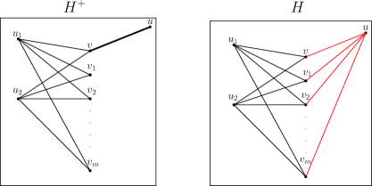
(a) $f(H)$ changes outside loop

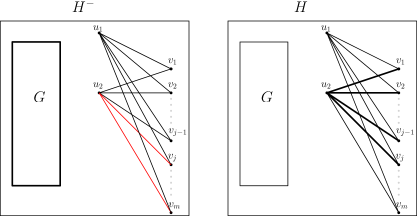
(b) $f(H)$ changes inside loop

Figure 2: Example with $\delta^{\prime}(G)=3$. Black lines are edges, thick black lines are sensitive edges, red lines are sensitive non-edges.

Case 2 ($\delta^{\prime}(G)=1$, $c(G)\geq 2$)

Let $G\in m(f)$ be a graph so that $\delta^{\prime}(G)=1$, $c(G)=c(f)$. Denote by $T_{1},\dots,T_{r}$ the connected components of $G$ that are trees but non isolated edges, by $C_{1},\dots,C_{l}$ the connected components that are non-trees, and by $I(G)=\{v_{1},\dots,v_{m}\}$ the set of isolated vertices. We do not assume a-priori that $c(G)<\infty$, that is, that $G$ has any components of the form $T_{i}$. However, we soon prove that this is indeed the case.

Notice, that for each component $T_{i}$ the number of edges in $T_{i}$ is exactly one less than the number of vertices in it, and for each component $C_{i}$ the number of edges in $C_{i}$ is at least the number of vertices in it. Summing over all components, we obtain

$$|I(G)|+|G|\geq n-r.$$ (7)

We show that $r\geq 3$. Since $G$ is minimal, and $\delta^{\prime}(G)=1$, by Lemma 3.1 $|I(G)|\leq s(f)-1\leq\frac{1}{2}n-2$. Yet, from that same minimality, $G$ is sensitive at every edge it contains, therefore
$|G|\leq s(f,G)\leq s(f)\leq\frac{1}{2}n-1$. Adding the two, we deduce $|I(G)|+|G|\leq n-3$, and so $r\geq 3$ by (7).

From the pigeonhole principle and the minimality of $G$,

$$c(G)\leq|G|/r<\frac{1}{2r}n.$$ (8)

In this particular case, we also assume $c(G)\geq 2$, so combined with (8) this implies $r<\frac{1}{4}n$.
We provide an algorithm which has as input a minimal graph $G$ with the properties described above, and outputs a graph $G^{\prime}\subseteq G$, $f(G^{\prime})=1$, which is a contradcition to the minimality of $G$. Recall, the set of isolated edges of $G$ is $I(G)=\{v_{1},\dots,v_{m}\}$.

Algorithm 2 Algorithm for $\delta^{\prime}(f)=1$, $c(f)\geq 2$

  $H\leftarrow G$

  Find some tree component $T=(V_{T},E_{T})$ of $G$ with $c(G)=|E(T)|$, and some construction sequence $T^{(1)},\dots,T^{(c(G))}$ of $T$.

  for $i:=1\to c(G)-1$ do

     if $\exists e\in G$ so that $f(H\setminus e)=f(H)$ then

        $H\leftarrow H\setminus e$

        return  some minimal graph $G^{\prime}\subset H$ {We prove that such $G^{\prime}$ must exist}

     end if

     connect vertex $v_{i+1}$ to some vertex $v_{j}$, $1\leq j\leq i$, so that the subgraph of $H$ induced on vertices $v_{1},\dots,v_{i+1}$ will be isomorphic to $T^{(i)}$.

  end for

  Remove from $H$ some edge $e=\{u,v\}$ in component $T$, so that $(V_{T}\setminus\{u\},E_{T}\setminus\{e\})$ is isomorphic to $T^{(c(G)-1)}$.

  return  some minimal graph $G^{\prime}\subset H$ {We prove that such $G^{\prime}$ must exist}

Claim 3.

At each stage in the algorithm $f(H)$=1. Thus, $f(G^{\prime})$=1.

Proof.

Assume that at some stage in the algorithm $f(H)=0$, and let us take the first time that this happens. This stage can either occur inside the for-loop, or after the for-loop, while removing edge $e=\{u,v\}$. Assume the former. The value of $f(H)$ can not change inside the if-condition, because the if-condition only holds if edge $e$ could be removed from $H$ without changing the value of $f$ in $H$.

From this it follows that the change occurs at some iteration, $i$, when adding the edge $\{v_{i+1},v_{j}\}$ for some $1\leq j\leq i$. Denote by $H^{-}=H\setminus\{v_{i+1},v_{j}\}$ the graph just before this edge was removed. $f(H^{-})=1$. Furthermore, no edge $e\in G$ could be removed from $H^{-}$ without changing the value of the function, otherwise the if-condition in the beginning of the $i$th iteration would hold. Hence, $H^{-}$ is sensitive on all $|G|$ edges that belong to $G$. In addition to that, $H$ is isomorphic to $H^{-}\cup\{v_{j},v_{l}\}$ for every $i+1\leq l\leq m$. Thus, adding any one of these edges to $H^{-}$ changes the value of $f$ on the graph. Together, we see that
$s(f)\geq s(f,H^{-})\geq m-i+|G|\geq m-c(G)+1+|G|$. From (7) and our assumption $s(f)\leq\frac{1}{2}n-1$, we obtain

$$\frac{1}{2}n\geq n-r-c(G)+2,$$ (9)

and recalling (8), we deduce

$$\frac{1}{2}n+2<r+\frac{n}{2r}.$$ (10)

This inequality does not hold for any $3\leq r\leq n/4$, and $n$ sufficiently large.

Next, assume that $f(H)$ becomes zero for the first time after the loop, while removing edge $\{u,v\}$. Denote by $H^{+}=H\cup\{u,v\}$, the graph just before removing edge $\{u,v\}$ and changing the value of the function. The following facts are of importance to us:

• $H$ contains two connected components, which are isomorphic to $T^{(c(G))-1}$. Namely, one copy on vertices $v_{1},\dots,v_{c(G)}$ with edges added by the algorithm, and one copy formed from $T$ by removing edge $\{u,v\}$. Call these copies $T_{1}$ and $T_{2}$, respectively.

• $I(H)=\{v_{c(G)+1},\dots,v_{m},u\}$, so

  $$|I(H)|=m-c(G)+1.$$ (11)

The graph $H^{+}$ is isomorphic to any graph of the form $H\cup\{v,w\}$, $w\in I(H)$. Additionally, there is some vertex $v_{j}\in V(T_{1})$, $1\leq j\leq c(G)$, so that for any $w\in I(H)$, $H\cup\{v_{j},w\}$ is isomorphic to $H^{+}$. This is true, because $T_{1}$ and $T_{2}$ are isomorphic. From all of the above, it follows that $\frac{1}{2}n>s(f,H)\geq 2|I(H)|$. With (8) and (11), this implies

$$\frac{1}{2}n>2(m-c(G)+1)\geq 2(m-|G|/r+1)$$ (12)

From equation (7), we know that $m\geq n-|G|-r$. Plugging this into (12), using $|G|\leq\frac{1}{2}n-1$, we have

$$\frac{1}{4}n>n-r-(\frac{1}{2}n-1)(1+\frac{1}{r})+1.$$ (13)

Reogranizing, using $r\geq 3$:

$$r-2>\frac{1}{4}n(1-\frac{1}{2r}),$$ (14)

or

$$r>n/4,$$ (15)

which we have shown is impossible. Thus, at every stage of the algorithm $f(H)=1$ (see Figure  3), and consequentially $f(G^{\prime})=1$. ∎

Claim 4.

$G^{\prime}\subsetneq G$

Proof.

Let $c(G)=k$. Notice that throughout the algorithm, $H_{(k)}\subseteq G=G_{(k)}$, because all edges which are in $H\setminus G$ form a tree component in $H$ with less than $k$ edges. The last change the algorithm does to $H$, is removing an edge from $H$ that is also an edge of $G$. Thus, after this edge is removed and the algorithm does not change $H$ anymore, it is the case that $H_{(k)}\subsetneq G$, hence also $G^{\prime}_{(k)}\subsetneq G$. Recall our choice of $G$: $G\in m(f)$ and $k=c(G)=c(f)$. $G^{\prime}\in m(f)$ as well, so of course $c(G^{\prime})\geq c(f)=k$, and therefore $G^{\prime}=G^{\prime}_{(k)}\subsetneq G$, proving the claim ∎

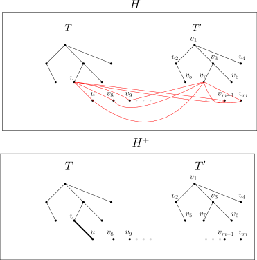
Figure 3: Example with $c(G)=7$, $f(H)$ changes outside loop. Black lines are edges, thick black lines are sensitive edges, red lines are sensitive non-edges.

Case 3 ($c(f)=1$)

Choose a graph $G\in m(f)$, so that $\delta^{\prime}(G)=1$, $c(G)=1$. Let $E_{1},\dots,E_{m}$ be its connected components with one edge, $C_{1},\dots,C_{l}$ the connected components with at least $2$ edges, and $I(G)=\{w_{1},\dots,w_{r}\}$ the set of isolated vertices. The following structural lemma will be useful:

Lemma 3.2.

For the graph $G$ above:

1. $r\geq 2$

2. $r=o(n)$

3. $m=\frac{1}{2}n-o(n)$ and $l=o(n)$

Proof.

1. Since $G$ is minimal, $|G|\leq s(f,G)\leq\frac{1}{2}n-1$. In any graph, the number of non-isolated vertices is at most twice the number of edges. Thus, $r\geq n-2|G|\geq n-(n-2)=2$.

2. Let $\{u,v\}\in E(G)$ be an edge which connects two vertices of degree one. Remove this edge, to obtain graph $G^{-}=G\setminus\{u,v\}$. By minimality of $G$, $f(G^{-})\neq f(G)$. $|I(G^{-})|=r+2$, and adding any edge between two isolated vertices in $G^{-}$ will create a graph isomorphic to $G$, and thus change the value of the function. Thus, ${r+2\choose 2}\leq s(f,G^{-})\leq s(f)\leq\frac{1}{2}n$, so $r=o(n)$.

3. Notice, that for each component $E_{i}$, $i\in[m]$, there are exactly two vertices in the component. Thus, the total number of vertices in these components is $2m$. For any component $C_{i}$, $i\in[l]$, $|V(C_{i})|\leq|C_{i}|+1\leq\frac{3}{2}|C_{i}|$, because $|C_{i}|\geq 2$. So we can write the following inequalites:

   $$\frac{1}{2}n-1\geq|G|=m+\sum_{i=1}^{l}|C_{i}|$$ (16)

   $$n=r+2m+\sum_{i=1}^{l}(|C_{i}|+1)\geq o(n)+2m+\frac{3}{2}\sum_{i=1}^{l}|C_{i}|.$$ (17)

   taking $4\cdot\eqref{edges}-2\cdot\eqref{vertices}$, we obtain

   $\sum_{i=1}^{l}|C_{i}|=o(n)$, and thus $m=\frac{1}{2}n-o(n)$, proving $3$.

∎

Our method of proof will be to obtain two isomorphic graphs $H$ and $H^{\prime}$, for which $f(H)\neq f(H^{\prime})$, which is impossible since $f$ is a graph property. Let $E_{i}=\{v_{i},u_{i}\}$, for $1\leq i\leq m$. We define $H=G\cup\{u_{1},u_{2}\}\cup(\bigcup_{i=3}^{\lceil n/6\rceil+1}\{v_{1},v_{i}\}$. Next, we define $H^{\prime}=H\cup\{v_{1},v_{2}\}\setminus\{u_{1},v_{1}\}$. Notice, that $H^{\prime}$ is isomorphic to $H$, since the function $\pi:V(H^{\prime})\to V(H)$ given by $\pi(v_{2})=u_{1}$, $\pi(u_{1})=v_{2}$, $\pi(x)=x$ for all $x\in V\setminus\{v_{2},u_{1}\}$ is a graph isomorphism. So to finish the proof, we just need to prove $f(H)\neq f(H^{\prime})$.

Claim 5.

$f(H)=1$.

Proof.

Construct $H$ from $G$ in the following way. First, add edge $\{u_{1},u_{2}\}$, and then add the edges $\{v_{1},v_{i}\}$ one by one, starting from $i=3$ and increasing $i$ by one each time. In this way we obtain a sequence of graphs $G:=G_{1},G_{2},G_{3},\dots,G_{\lceil n/6\rceil+1}=H$, so that $G_{2}=G\cup\{u_{1},u_{2}\}$, and for
$3\leq i\leq\lceil n/6\rceil+1$, $G_{i}=G_{i-1}\cup\{v_{1},v_{i}\}$.

Notice that $G_{2}$ is isomorphic to $G\cup\{u_{i},u_{j}\}$ for any $1\leq i<j\leq m$, and so if $G$ was sensitive for $\{u_{1},u_{2}\}$ it would be sensitive for $\Omega(m^{2})=\Omega(n^{2})$ edges, which is impossible for sufficiently large $n$. So $f(G_{1})=1$. Assume that $G_{i}$ is the first graph in the sequence for which $f(G_{i})=0$, for some $3\leq i\leq\lceil n/6\rceil+1$. That is, $G_{i-1}$ is sensitive on edge $\{v_{1},v_{i}\}$.

However, all graphs of the form $G_{i-1}\cup\{v_{1},v_{j}\}$ and $G_{i-1}\cup\{v_{1},u_{j}\}$ are isomorphic to $G_{i}$, for $i\leq j\leq m$. Hence, $s(f,G_{i-1})\geq 2(m-i+1)\geq 2(m-\lceil n/6\rceil)=\frac{2}{3}n-o(n)>\frac{1}{2}n$, for sufficiently large $n$. This contradicts our assumption $s(f)\leq\frac{1}{2}n-1$. Hence, $f(H)=f(G)=1$. ∎

Claim 6.

$f(H^{\prime})=0$.

Proof.

Since $G$ is minimal, $f(G\setminus\{u_{1},v_{1}\})=0$. Denote by $G^{\prime}=G\setminus\{u_{1},v_{1}\}$. $u_{1},v_{1}\in I(G^{\prime})$, because they both belong to $E_{1}$ in $G$. Thus, $|I(G^{\prime})|=r+2\geq 4$, from $1$ in lemma 3.2. Construct $H^{\prime}$ from $G^{\prime}$, by first adding edges $\{v_{1},v_{i}\}$ one by one, starting from $i=2$ and increasing $i$ by one each time. Finally, add the edge $\{u_{1},u_{2}\}$.

In this way we obtain a sequence of graphs $G^{\prime}:=G^{\prime}_{1},G^{\prime}_{2},\dots,G^{\prime}_{\lceil n/6\rceil+1},H^{\prime}$, so that $G^{\prime}_{i}=G^{\prime}_{i-1}\cup\{v_{1},v_{i}\}$ for every $2\leq i\leq\lceil n/6\rceil+1$, and $H=G^{\prime}_{\lceil n/6\rceil+1}\cup\{u_{1},u_{2}\}$. From identical consideration as in the previous claim, $f(G_{i})=f(G_{i-1})=0$ for all $2\leq i\leq\lceil n/6\rceil+1$, since otherwise $G_{i-1}$ would be sensitive for too many edges.

Thus, we just need to prove $f(H^{\prime})=f(G_{\lceil n/6\rceil+1})$. Denote by $H^{\prime-}=G^{\prime}_{\lceil n/6\rceil+1}$. the only vertex that is isolated in $G^{\prime}$ but not in $H^{\prime-}$ is $v_{1}$. So let $u_{1},w_{1},w_{2}\in I(H^{\prime-})$. Notice that $H^{\prime}$ is isomorphic to all graphs of the form $H^{\prime-}\cup\{u_{1},u_{j}\}$, $H^{\prime-}\cup\{w_{1},u_{j}\}$, $H^{\prime-}\cup\{w_{2},u_{j}\}$, for $2\leq j\leq\lceil n/6\rceil+1$. This makes a total of $3\lceil n/6\rceil>\frac{1}{2}n-1\geq s(f)$, so if $f(H^{\prime-})\neq f(H^{\prime})$, then $s(f,H^{\prime-})>s(f)$, which is impossible. Hence, $f(H^{\prime})=0$, proving the claim. ∎

∎

4 Concluding Remarks

Conjecture 1 remains unresolved, more than thirty years after it was first formulated. This author remains agnostic about the veracity of the conjecture.

One can of course ask an analogous question for $k$-uniform hypergraphs for any fixed integer $k\geq 2$. That is, is the minimum sensitivity for any non-trivial $k$-uniform hypergraph property the same as the minimum sensitivity for any non-trivial monotone $k$-uniform hypergraph property. It turns out, though, that for $k>2$ this is false, even asymptotically.

Indeed, it is well known, and not hard to see, that if $f$ is a non-trivial monotone $k$-uniform hypergraph property, then $s(f)=\Omega(n^{k/2})$. On the other hand, in a paper recently uploaded to arxiv, Li and Sun [7] show that for any $k\geq 2$, there exists a non-trivial $k$-uniform hypergraph property so that

$$s(f)=O(n^{\lceil k/3\rceil}),$$ (18)

and if $k\equiv 1(\textrm{mod}\ 3)$, this bound can be improved to

$$s(f)=O(n^{\lceil k/3\rceil-1/2}).$$ (19)

Regardless, bounds for the sensitivity of $k$-uniform hypergraph properties remain of interest, both for the monotone and for the general case.

Finally, we propose a weaker form of Conjecture 1, where we limit $f$ to be a non-trivial min-term graph property. See [3] for the definition of a min-term function.

Conjecture 2.

Let $f:\{0,1\}^{n\choose 2}\to\{0,1\}$ be a non-trivial min-term graph property. Then

$$s(f)\geq n-1.$$

References

- [1] A. Ambainis: Polynomial degree vs. quantum query complexity, J. of Computer and Systems Sciences, 72(2) (2006), 220-238.
- [2] R. Beals, H. Buhrman, R. Cleve, M. Mosca and R. De Wolf: Quantum lower bounds by polynomials, J. ACM, 48(4) (2001), pages 778-797.
- [3] S. Chakraborty: On the Sensitivity of Cyclically-Invariant Boolean Functions, CCC 2005, pages 163-167.
- [4] S. Cook and C. Dwork: Bounds on the time for parallel RAM’s to compute simple functions, STOC 1982, pages 231-233.
- [5] Y. Gao, J. Mao, X. Sun and S. Zuo: On the sensitivity complexity of bipartite graph properties, Theoretical Computer Science 468 (2013), 83-91.
- [6] P. Hatami, R. Kulkarni and D. Pankratov: Variations on the sensitivity conjecture, Theory of Computing, Graduate Surveys4 (2011), 1-27
- [7] Q. Li and X. Sun: On the Sensitivity Complexity of -Uniform Hypergraph Properties, https://arxiv.org/abs/1608.06724 (2016), 15 pages.
- [8] C. Kenyon and S. Kutin: Sensitivity, block sensitivity and -block sensitivity of boolean functions, Information and Computation 189 http://arxiv.org/abs/1507.02242.
- [9] N. Nisan: CREW PRAMs and decision trees, 1989 STOC,(1997), 327-335.
- [10] N. Nisan and M. Szegedy: On the degree of Boolean functions as real polynomials, Computational Complexity 4(4) (1994), pages 301-313.
- [11] D. Rubinstein: Sensitivity vs. block sensitivity of Boolean functions, Combinatorica, 4(2) (1995), 297-299.
- [12] H. Simon: A Tight -Bound on the Time for Parallel Ram’s to Compute Nondegenerated Boolean Functions, FCT 1983, pages 439-444.
- [13] X. Sun: An improved lower bound on the sensitivity complexity of graph properties, Theoretical Computer Science 412(29)(2011), 3524-3529.
- [14] X. Sun: Block sensitivity of weakly symmetric functions, Theoretical Computer Science, 384(1) (2007), 87-91.
- [15] Gy. Turan: The critical complexity of graph properties, Inforamtion Processing Letters 18(3) (1984), 151-153.
- [16] I. Wegener: The critical complexity of all (monotone) Boolean functions and monotone graph properties, FCT 1985, pages 494-502.