Solving ill-posed control problems by stabilized finite element methods: an alternative to Tikhonov regularization

Abstract.

Tikhonov regularization is one of the most commonly used methods of regularization of ill-posed problems. In the setting of finite element solutions of elliptic partial differential control problems, Tikhonov regularization amounts to adding suitably weighted least squares terms of the control variable, or derivatives thereof, to the Lagrangian determining the optimality system. In this note we show that stabilization methods for discretely ill–posed problems developed in the setting of convection–dominated convection–diffusion problems, can be highly suitable for stabilizing optimal control problems, and that Tikhonov regularization will lead to less accurate discrete solutions. We consider data assimilation problems for Poisson’s equation as illustration and derive new error estimates both for the the reconstruction of the solution from measured data and reconstruction of the source term from measured data. These estimates include both the effect of discretization error and error in measurements.

Keywords: optimal control problem, source identification, finite elements, regularization

1. Introduction

In this note we propose an alternative to the classical Tikhonov regularization approach in finite element approximations of optimal control problems governed by elliptic partial differential equations. We shall, following [2], consider problems of the type

(1) $$J(u,q)\rightarrow\text{min!},\quad A(u)=f+B(q),$$

where $J$ is a cost functional, $A$ is an elliptic differential operator for the state variable $u$, and $B$ an impact operator for the control variable $q$. Introducing costate variables $\lambda$, this problem can be formulated as finding saddle points to the Lagrangian functional

(2) $${\mathfrak{L}}(u,q,\lambda):=J(u,q)+(\lambda,A(u)-f-B(q)),$$

where $(\cdot,\cdot)$ denotes the $L_{2}$ inner product, determined by the system

(3) $$\left\{\begin{array}[]{>{\displaystyle}l}\frac{d}{d\epsilon_{1}}\left.{\mathfrak{L}}(u+\epsilon_{1}v,q,\lambda)\right|_{\epsilon_{1}=0}=0,\\[5.69054pt] \frac{d}{d\epsilon_{2}}\left.{\mathfrak{L}}(u,q+\epsilon_{2}r,\lambda)\right|_{\epsilon_{2}=0}=0,\\[5.69054pt] \frac{d}{d\epsilon_{3}}\left.{\mathfrak{L}}(u,q,\lambda+\epsilon_{3}\mu)\right|_{\epsilon_{3}=0}=0.\\[5.69054pt] \end{array}\right.$$

In a finite element setting, the continuous states, controls, and costates $(u,q,\lambda)\in V\times Q\times V$ are replaced by their discrete counterparts $(u^{h},q^{h},\lambda^{h})\in V^{h}\times Q^{h}\times V^{h}$, where $V^{h}$ and $Q^{h}$ are finite dimensional counterparts of the appropriate Hilbert spaces $V$ and $Q$, respectively.

Typically, the cost functional measures some distance between the discrete state and a known or sampled function $u_{0}$ over a subdomain $\mathcal{M}\subseteq\Omega$ where $\Omega\subset\mathbb{R}^{d}$, $d=2,3$ is a polyhedral (polygonal) domain of computation.

(4) $$J(u,q):=\frac{1}{2}\|u-u_{0}\|^{2}_{\mathcal{M}}$$

which may not lead to a well posed problem. A classical regularization method due to Tikhonov, see [11], is to add a stabilizing functional $n(q,q)$,

(5) $$J(u,q):=\frac{1}{2}\|u-u_{0}\|^{2}_{\mathcal{M}}+n(q,q),$$

where, typically,

(6) $$n(q,q):=\alpha\|q-q_{b}\|^{2}+\beta\|\nabla(q-q_{b})\|^{2},$$

with $\alpha$ and $\beta$ regularization parameters and $q_{b}$ the background state, or first guess state. The role of the background state is to diminuish the nonconsistent character of the Tikhonov regularization and implies additional a priori knowledge on the system beyond the samples $u_{0}$. In this note we will assume that no such additional a priori data are at hand, $q_{b}=0$ and that there is no physical justification for the addition of the term $n(q,q)$, or that the size of $\alpha$ and $\beta$ given by the application are too small to provide sufficient stabilization of the system for computational purposes. The objective of this note is to show that these regularizations can be improved upon in a finite element framework. The approach that we will follow is to eliminate the Tikhonov regularization on the continuous level and instead regularize the discrete formulation hence making the regularization part of the computational method in the form of a weakly consistent stabilization.

The terminology stabilization versus regularization is slightly ambiguous but in classical numerical analysis the method of modified equations [10] provides a link between these concepts.

1.1. Model problems

We will discuss two model problems below. First let $\mathcal{M}\subset\Omega$ be a ball $B_{r_{1}}(\bf{x}_{0})$ with radius $r_{1}$, centered at $\bf{x}_{0}$ and assume that measurements $u_{0}$ are available in this ball. We then wish to reconstruct the solution $u$ in $B_{r_{2}}({\bf{x}}_{0})$ under the a priori assumption that $B_{r_{2}}({\bf{x}}_{0})\subset B_{r_{3}}({\bf{x}}_{0})\subset\Omega$ and $u\in H^{1}(\Omega)$, is a weak solution to

$$-\Delta u=f,\mbox{ in }\Omega.$$

This problem can be cast in the form of a constrained minimization problem:

(7) $$\frac{1}{2}\|u-u_{0}\|^{2}_{L_{2}(\mathcal{M})}+\frac{\alpha}{2}\|\nabla u\|^{2}_{L_{2}(\Omega)}$$

subject to

(8) $$-\Delta u=f,\mbox{ in }\Omega.$$

We will refer to this problem as the data assimilation problem below, but it is also strongly related to boundary control problems. It is known that in this case if for $\alpha=0$ $u_{0}$ is such that a solution exists, then by unique continuation of harmonic functions this solution is unique. This statement can be quantified in the following three sphere’s inequality:

Lemma 1.

(Three spheres inequality) Assume that $u:\Omega\rightarrow\mathbb{R}$ is a weak solution of (8) with $f\in H^{-1}(\Omega)$ such that $\|f\|_{H^{-1}(\Omega)}\leq\varepsilon$ for some $\varepsilon>0$. For every $r_{1},\,r_{2},\,r_{3},\,\overline{r}$ such that $0<r_{1}<r_{2}<r_{3}<\overline{r}$ and for every ${\bf{x}}_{0}\in\Omega$ such that $\mbox{dist}({\bf{x}}_{0},\partial\Omega)>\overline{r}$ there holds

(9) $$\|u\|_{L^{2}(B_{r_{2}})}\leq C\left(\|u\|_{L^{2}(B_{r_{1}})}+\varepsilon\right)^{\tau}\cdot\left(\|u\|_{L^{2}(B_{r_{3}})}+\varepsilon\right)^{(1-\tau)}$$

where $B_{r_{i}}$, $i=1,2,3$ are balls centered at ${\bf{x}}_{0}$, $C>0$ and $\tau$, $0<\tau<1$ only depend on the geometry of $\Omega$, and the ratios $r_{2}/r_{1}$ and $r_{3}/r_{2}$.

Proof.

For a proof in the non-homogeneous case considered here see Allessandrini et al. [1, Theorem 1.10]. ∎

Remark 1.

We do not track the exact form of the geometric constants that appear in the proof of Lemma 1. They are all considered included in the canonical constant $C$ above. For the precise definition of the result with all exact dependencies we refer to [1].

Assume that $\Omega\subset\mathbb{R}^{d}$ with $B_{r_{3}}(\bf{x}_{0})\subset\Omega$. Introducing the Lagrange multiplier $\lambda\in H^{1}_{0}(\Omega)$, we have the optimality system: find $(u,\lambda)\in H^{1}(\Omega)\times H^{1}_{0}(\Omega)$ such that

(10) $$\int_{\mathcal{M}}u\,v\,d\Omega+\int_{\Omega}\nabla\lambda\cdot\nabla v\,d\Omega=\int_{\mathcal{M}}u_{0}\,v\,d\Omega\quad\forall v\in H^{1}(\Omega),$$

(11) $$\int_{\Omega}\nabla u\cdot\nabla\mu\,d\Omega=\int_{\Omega}f\,\mu\,d\Omega\quad\forall\mu\in H^{1}_{0}(\Omega).$$

The difficulty in this case is that the equation (11) is ill-posed, since $u\in H^{1}(\Omega)$ and $\mu\in H^{1}_{0}(\Omega)$. It follows that coercivity fails for $u$ in $H^{1}(\Omega)$. Clearly this is not the case when $\alpha>0$, but then a nonconsistent perturbation is added to the system that can not easily be quantified. Below we will instead add a regularization on the discrete level. Indeed we will penalize the fluctuations of the gradient over element faces and show that the added coercivity on the high frequency content of the solution is sufficient to obtain a priori estimates leading to error estimates through Lemma 1. This part of the analysis draws on earlier ideas for the elliptic Cauchy problem from [4, 5]. Below we will assume that $u_{0}$ is the unperturbed measurement for which the unique solution exists and consider a numerical method with perturbed data.

Our second example considers the case where the data is available in the whole domain, $\mathcal{M}\equiv\Omega$, but the source term is unknown and must be reconstructed. The challenge here being that the application of the Laplacian is unstable. This case will be referred to as source reconstruction below, but is also related to a distributed control problem. We consider the elementary problem: minimize

(12) $$\frac{1}{2}\|u-u_{0}\|^{2}_{L_{2}(\Omega)}+\frac{\alpha}{2}\|q\|^{2}_{L_{2}(\Omega)}$$

subject to

(13) $$\text{$-\Delta u=q$ in $\Omega$, $u=0$ on $\partial\Omega$}.$$

Here, $u_{0}$ is known data and $\Omega$ is a convex polygonal (polyhedral) subset of $\mathbb{R}^{d}$, $d=2,3$, with outword pointing normal $n$. We assume that we wish to solve (12)-(13) in the situation where $u_{0}$ is a measurement on a system that is of the form (13). This means that if no perturbations are present in the data and measurements are available in every point of $\Omega$, the minimizer for $\alpha=0$ is $u=u_{0}\in H^{1}_{0}(\Omega)\cap H^{2}(\Omega)=:W$ and an associated $q=-\nabla^{2}u\in L^{2}(\Omega)$ exists so that (13) is satisfied. Assume also that the shift theorem $\|u\|_{H^{2}(\Omega)}\leq C\|q\|_{L^{2}(\Omega)}$ holds. Below we will consider the problem of reconstructing $q$ from $u_{0}$ accounting for both the discretization error and the error due to errors in the measured data $u_{0}$.

Introducing the Lagrange multiplier $\lambda\in H^{1}_{0}(\Omega)$, we have the optimality system: find $(u,q,\lambda)\in H^{1}_{0}(\Omega)\times L_{2}(\Omega)\times H^{1}_{0}(\Omega)$ such that

(14) $$\int_{\Omega}u\,v\,d\Omega+\int_{\Omega}\nabla\lambda\cdot\nabla v\,d\Omega=\int_{\Omega}u_{0}\,v\,d\Omega\quad\forall v\in H^{1}_{0}(\Omega),$$

(15) $$\alpha\int_{\Omega}q\,r\,d\Omega+\int_{\Omega}\lambda\,r\,d\Omega=0\quad\forall r\in L_{2}(\Omega),$$

(16) $$\int_{\Omega}\nabla u\cdot\nabla\mu\,d\Omega=\int_{\Omega}q\,\mu\,d\Omega\quad\forall\mu\in H^{1}_{0}(\Omega).$$

We note here that the trace of $\lambda$ is zero on the boundary but that this does not affect $q$ in the infinite dimensional case. However, when we discretize and solve for discrete counterparts ($u^{h},\lambda^{h},q^{h}$), a problem arises in that the finite dimensionality of the problem forces the zero boundary condition on $\lambda^{h}$ onto $q^{h}$ via the $L_{2}$–projection in (15). This has profound implications for the accuracy close to the boundary of the control $q^{h}$. As a remedy for this we propose to introduce the regularization of $q$ in the discrete setting so that it acts only on fluctuations of the gradient of the source term, with a particular scaling in the mesh-size. Since the kernel of this operator is so big, the stability of the system (14)-(16) is compromised. We therefore also introduce a stabilization of the type suggested above, where the jumps of the gradient of $u$ are penalized as well. This is sufficient to make the system inf-sup stable in a suitable discrete norm as we shall see below.

2. Derivation of the discrete model

Let $\{\mathcal{T}_{h}\}_{h}$ denote a family of shape regular and quasi uniform tesselations of $\Omega$ into nonoverlapping simplices, such that for any two different simplices $K$, $K^{\prime}\in\mathcal{T}_{h}$, $K\cap K^{\prime}$ consists of either the empty set, a common face/edge or a common vertex. The outward pointing normal of a simplex $K$ will be denoted $n_{K}$. We denote the set of interior element faces $F$ in $\mathcal{T}_{h}$ by $\mathcal{F}_{I}$. To each face we associate a normal $n_{F}$ whose orientation is arbitrary but fixed. We define the standard finite element space of continuous piecewise affine functions on $\mathcal{T}_{h}$

$$V_{h}:=\{v_{h}\in C^{0}(\overline{\Omega}):v_{h}|_{K}\in P_{1}(K),\,\forall K\in\mathcal{T}_{h}\},$$

where $P_{1}(K)$ denotes the set of affine functions on $K$. We also define $V_{h}^{0}:=V_{h}\cap H^{1}_{0}(\Omega)$.

2.1. Data assimilation

Consider the discrete formulation: find $u_{h},\lambda_{h}\in V_{h}\times V_{h}^{0}$ such that

(17) $$m_{\mathcal{M}}(u_{h},v_{h})+s_{1}(u_{h},v_{h})+a_{h}(v_{h},\lambda_{h})=m_{\mathcal{M}}(\tilde{u}_{0},v_{h})\quad\forall v_{h}\in V_{h},$$

(18) $$a_{h}(u_{h},\mu_{h})=m_{\Omega}(\tilde{f},\mu_{h})\quad\forall\mu_{h}\in V_{h}^{0},$$

where $\tilde{f}:=f+\delta f$ and $\tilde{u}_{0}:=u_{0}+\delta u_{0}$, with $\delta f\in H^{-1}(\Omega)$ and $\delta u_{0}\in L^{2}(\mathcal{M})$ denote measurement errors in the source term and data. The bilinear forms are given by

(19) $$m_{X}(u_{h},v_{h}):=\int_{X}u_{h}\,v_{h}\,d\Omega,\mbox{ for }X\subseteq\Omega,$$

(20) $$s_{i}(u_{h},v_{h}):=\sum_{F\in\mathcal{F}_{I}}\gamma\int_{F}h^{i}_{F}\llbracket\nabla u_{h}\cdot n_{F}\rrbracket\llbracket\nabla v_{h}\cdot n_{F}\rrbracket~{}\mbox{d}s$$

where $\llbracket y_{h}\rrbracket|_{F}:=\lim_{\epsilon\rightarrow 0^{+}}(y_{h}(x-\epsilon n_{F})-y_{h}(x+\epsilon n_{F}))$ denotes the jump of the quantity $y_{h}$ over the face $F$, with normal $n_{F}$ and finally

(21) $$a_{h}(v_{h},\lambda_{h}):=\int_{\Omega}\nabla v_{h}\cdot\nabla\lambda_{h}\,d\Omega.$$

This may then be written on the compact form, find $u_{h},\lambda_{h}\in\mathcal{V}^{DA}_{h}$, with $\mathcal{V}^{DA}_{h}:=V_{h}\times V_{h}^{0}$ such that

$$A_{DA}[(u_{h},\lambda_{h}),(v_{h},\mu_{h})]=m_{\Omega}(\tilde{f},\mu_{h})+m_{\mathcal{M}}(\tilde{u}_{0},v_{h}),\quad\forall v_{h},\mu_{h}\in\mathcal{V}^{DA}_{h},$$

with

$$\begin{array}[]{ll}A_{DA}[(u_{h},\lambda_{h}),(v_{h},\mu_{h})]:=&m_{\mathcal{M}}(u_{h},v_{h})+s_{1}(u_{h},v_{h})\\[5.69054pt] &+a_{h}(v_{h},\lambda_{h})+a_{h}(u_{h},\mu_{h}).\end{array}$$

2.2. Source reconstruction

Consider the discrete formulation: find $u_{h},q_{h},\lambda_{h}\in V_{h}^{0}\times V_{h}\times V_{h}^{0}$ such that

(22) $$m(u_{h},v_{h})+s_{1}(u_{h},v_{h})+a_{h}(v_{h},\lambda_{h})=m(u_{0},v_{h})\quad\forall v_{h}\in V_{h}^{0},$$

(23) $$m(\lambda_{h},w_{h})-s_{5}(q_{h},w_{h})=0\quad\forall w_{h}\in V_{h}$$

and

(24) $$a_{h}(u_{h},\mu_{h})=m(q_{h},\mu_{h})\quad\forall\mu_{h}\in V_{h}^{0}.$$

with bilinear forms given by (19), (20) and (21) above. Below we will distinguish the stabilization parameters of $s_{1}(\cdot,\cdot)$ and $s_{5}(\cdot,\cdot)$ and then denote them by $\gamma_{1}$ and $\gamma_{5}$ respectively.

This may then be written on the compact form, find $u_{h},q_{h},\lambda_{h}\in\mathcal{V}_{h}^{SR}$, with $\mathcal{V}_{h}^{SR}:=V_{h}^{0}\times V_{h}\times V_{h}^{0}$ such that

$$A_{SR}[(u_{h},q_{h},\lambda_{h}),(v_{h},w_{h},\mu_{h})]=m(u_{0},v_{h}),\quad\forall v_{h},\,r_{h},\,\mu_{h}\in\mathcal{V}_{h}^{SR},$$

with

$$\begin{array}[]{ll}A_{SR}[(u_{h},q_{h},\lambda_{h}),(v_{h},w_{h},\mu_{h})]:=&m(u_{h},v_{h})+s_{1}(u_{h},v_{h})\\[5.69054pt] &+a_{h}(v_{h},\lambda_{h})+s_{5}(q_{h},w_{h})-m(\lambda_{h},w_{h})\\[5.69054pt] &-a_{h}(u_{h},\mu_{h})+m(q_{h},\mu_{h}).\end{array}$$

3. Preliminary technical results

First we define the semi norms associated with the stabilization operator $s_{i}(\cdot,\cdot)$,

$$|x_{h}|_{s_{i}}=s(x_{h},x_{h})^{\frac{1}{2}},\quad\forall x_{h}\in V_{h}.$$

We recall the following well known inverse and trace inequalities

(25) $$\begin{array}[]{rcl}\|v\|_{L^{2}(\partial K)}\leq C_{t}(h^{-\frac{1}{2}}\|v\|_{K}+h^{\frac{1}{2}}\|\nabla v\|_{K}),\quad\forall v\in H^{1}(K)\\[5.69054pt] h_{K}\|\nabla v_{h}\|_{K}+h_{K}^{\frac{1}{2}}\|v_{h}\|_{L^{2}(\partial K)}\leq C_{i}\|v_{h}\|_{K},\quad\forall v_{h}\in V_{h}.\end{array}$$

As an immediate consequence of (25) we have the following stabilities for some $C_{si}>0$ depending only on the mesh geometry,

(26) $$|x_{h}|_{s_{i}}\leq C_{si}\|h^{\frac{i-3}{2}}x_{h}\|_{L^{2}(\Omega)},\quad|x_{h}|_{s_{i}}\leq C_{si}\|h^{\frac{i-1}{2}}\nabla x_{h}\|_{L^{2}(\Omega)}.$$

Let $i_{h}:H^{2}(\Omega)\rightarrow V_{h}$ denote the standard Lagrange interpolant and $\pi_{h}:L^{2}\rightarrow V_{h}$ and $\pi^{0}_{h}:L^{2}\rightarrow V^{0}_{h}$ the $L^{2}$-projections on the respective finite element spaces. The following error estimate is known to hold both for $i_{h}$ and $\pi_{h}$,

(27) $$\|u-i_{h}u\|_{L^{2}(\Omega)}+h\|\nabla(u-i_{h}u)\|_{L^{2}(\Omega)}\leq Ch^{t}|u|_{H^{t}(\Omega)},\,t=1,2.$$

To prove stability of our formulations below we need to show that for any function $v_{h}\in V_{h}$ the $L^{2}$-norm is equivalent to $\|\pi^{0}_{h}v_{h}\|_{L^{2}(\Omega)}+|v_{h}|_{s_{3}}.$ We prove this result in this technical Lemma.

Lemma 2.

There exists $C_{p}>0$ such that for all $v_{h}\in V_{h}$ there holds

(28) $$h\|v_{h}\|_{H^{1}(\Omega)}\leq C_{p}(\|v_{h}\|_{L^{2}(\mathcal{M})}+|v_{h}|_{s_{1}}).$$

There exists $c_{1},c_{2}>0$ such that for any function $v_{h}\in V_{h}$

(29) $$c_{1}(\|\pi^{0}_{h}v_{h}\|_{L^{2}(\Omega)}+|v_{h}|_{s_{3}})\leq\|v_{h}\|_{L^{2}(\Omega)}\leq c_{2}(\|\pi^{0}_{h}v_{h}\|_{L^{2}(\Omega)}+|v_{h}|_{s_{3}}).$$

Proof.

The discrete Poincaré type inequality (28) may be proved using a compactness argument similar to that of [8]. To keep down the technical detail we here instead use an approach with continuous Poincaré inequalities and discrete interpolation. Let $\mathcal{I}_{h}:\nabla V_{h}\mapsto[V_{h}]^{d}$ be a quasi-interpolation operator [6] such that

(30) $$\|\nabla v_{h}-\mathcal{I}_{h}\nabla v_{h}\|_{L^{2}(\Omega)}\leq C|v_{h}|_{s_{1}},\quad\|\mathcal{I}_{h}\nabla v_{h}\|_{L^{2}(K)}\leq C\|\nabla v_{h}\|_{L^{2}(\Delta_{K})}$$

where $\Delta_{K}:=\cup_{K^{\prime}:K\cap K\neq\emptyset}$. The following Poincaré inequality is well known (see [9, Lemma B.63]). If $f:H^{1}(\Omega)\mapsto\mathbb{R}$ is a linear functional that is non-zero for constant functions then

$$\|u\|_{H^{1}(\Omega)}\leq C_{P}(|f(u)|+\|\nabla u\|_{L^{2}(\Omega)}),\quad\forall u\in H^{1}(\Omega).$$

For instance, we may take

$$f(u)=\int_{\mathcal{M}}u~{}\mbox{d}\Omega\leq C\|u\|_{L^{2}(\mathcal{M})}.$$

As an immediate consequence we have the bound

(31) $$\|v_{h}\|_{H^{1}(\Omega)}\leq C(\|v_{h}\|_{L^{2}(\mathcal{M})}+\|\nabla v_{h}\|_{L^{2}(\Omega)}).$$

Now let $\mathcal{M}_{int}\subset\mathcal{M}$, be the set $\mathcal{M}_{int}:=\{K\subset\mathcal{M},\,\partial K\cap\partial\mathcal{M}=\emptyset\}$, that is the set of interior triangles of $\mathcal{M}$. It then follows by the stability of $\mathcal{I}_{h}$ that $\|\mathcal{I}_{h}\nabla v_{h}\|_{L^{2}(\mathcal{M}_{int})}\leq C\|\nabla v_{h}\|_{L^{2}(\mathcal{M})}$. Adding and subtracting $\mathcal{I}_{h}\nabla v$ in the second term on the right hand side of (31) gives

(32) $$\|v_{h}\|_{H^{1}(\Omega)} \leq C(\|v_{h}\|_{L^{2}(\mathcal{M})}+\|\nabla v_{h}-\mathcal{I}_{h}\nabla v_{h}\|_{L^{2}(\Omega)}+\|\mathcal{I}_{h}\nabla v_{h}\|_{L^{2}(\Omega)})$$

$$\leq C(\|v_{h}\|_{L^{2}(\mathcal{M})}+|v_{h}|_{s_{1}}+\|\mathcal{I}_{h}\nabla v_{h}\|_{L^{2}(\Omega)})$$

where we used (30) in the second inequality. For the third term on the right hand side of (32) we once again use Poincaré’s inequality, the stability of $\mathcal{I}_{h}$ and the inverse inequality (25) to conclude that

$$\|\mathcal{I}_{h}\nabla v_{h}\|_{L^{2}(\Omega)} \leq C(\|\mathcal{I}_{h}\nabla v_{h}\|_{L^{2}(\mathcal{M}_{int})}+\|\nabla\mathcal{I}_{h}\nabla v_{h}\|_{L^{2}(\Omega)})$$

$$\leq C(h^{-1}\|v_{h}\|_{L^{2}(\mathcal{M})}+\|\nabla\mathcal{I}_{h}\nabla v_{h}\|_{L^{2}(\Omega)})$$

Using the fact that $\nabla v_{h}$ is constant on each element, so that

$$\|\nabla\mathcal{I}_{h}\nabla v_{h}\|^{2}_{L^{2}(\Omega)}=\sum_{K\in\mathcal{T}_{h}}\|\nabla(\nabla v_{h}-\mathcal{I}_{h}\nabla v_{h})\|^{2}_{L^{2}(K)}\leq Ch^{-2}\|\nabla v_{h}-\mathcal{I}_{h}\nabla v_{h}\|^{2}_{L^{2}(\Omega)}\leq Ch^{-2}|v_{h}|_{s_{1}}^{2}$$

where in the second inequality we have applied the inverse inequality (25) to each term in the sum, and finally used (30). We thus obtain

$$\|\mathcal{I}_{h}\nabla v_{h}\|_{L^{2}(\Omega)}\leq Ch^{-1}(\|v_{h}\|_{L^{2}(\mathcal{M})}+|v_{h}|_{s_{1}})$$

which combined with (32) gives

$$h\|v_{h}\|_{H^{1}(\Omega)} \leq C(h+1)(\|v_{h}\|_{L^{2}(\mathcal{M})}+|v_{h}|_{s_{1}})\leq C(\|v_{h}\|_{L^{2}(\mathcal{M})}+|v_{h}|_{s_{1}}).$$

By which we have proven (28).

The lower bound of (29) is immediate by the stability of the $L^{2}$-projection and the inverse and trace inequalities of equation (25). To prove the upper bound we write

$$\|v_{h}\|^{2}_{L^{2}(\Omega)}=\|\pi^{0}_{h}v_{h}\|^{2}_{L^{2}(\Omega)}+\|v_{h}-\pi^{0}_{h}v_{h}\|^{2}_{L^{2}(\Omega)}$$

and let $w_{h}:=v_{h}-\pi^{0}_{h}v_{h}$. We will now prove that

(33) $$\|w_{h}\|_{L^{2}(\Omega)}^{2}\leq|w_{h}|_{s_{3}}^{2}$$

from which the upper bound follows, since by the triangle inequality followed by the first inequality of (26), with $i=3$,

$$|w_{h}|_{s_{3}}\leq|v_{h}|_{s_{3}}+|\pi^{0}_{h}v_{h}|_{s_{3}}\leq|v_{h}|_{s_{3}}+C_{si}\|\pi^{0}_{h}v_{h}\|_{L^{2}(\Omega)}.$$

To prove (33) we first define the support of a nodal basisfunctions $\varphi_{i}$ by $\Omega_{i}:=\{x\in\Omega:\varphi_{i}(x)>0\}$. Then let $\mathcal{N}_{I}$ denote the set of indices of basis functions that are in the interior of the domain, that is, for each value $i\in\mathcal{N}_{I}$ the closure of the support of the associated basis function has empty intersection with the boundary, $\overline{\Omega}_{i}\cap\partial\Omega=\emptyset$. For each $i\in\mathcal{N}_{I}$ we define the macropatch $\Delta_{i}:=\cup_{j:\Omega_{j}\cap\Omega_{i}\neq\emptyset}\Omega_{j}$. This means that $\Delta_{i}$ consist of $\Omega_{i}$ and any other patch $\Omega_{j}$ sharing two triangles (in 2D) or several tetrahedra (in 3D) with $\Omega_{i}$. Since $\mathcal{T}_{h}$ is shape regular we may map the patch $\Delta_{i}$ to a shape regular $\tilde{\Delta}_{i}$ such that $\mbox{diam}(\tilde{\Delta}_{i})=1$. We define the linear map $F:\Delta_{i}\mapsto\tilde{\Delta}_{i}$. Let $\tilde{\mathcal{F}}$ and $\tilde{\mathcal{N}}$ denote the set of interior faces and interior nodes respectively of $\tilde{\Delta}_{i}$ and define the scalar product on $\tilde{\Delta}_{i}$

$$(\tilde{v}_{h},\tilde{y}_{h})_{\tilde{\Delta}_{i}}:=\int_{\tilde{\Delta}_{i}}\tilde{v}_{h}\tilde{y}_{h}|F^{-1}|\mbox{d}\tilde{x}.$$

It follows that if $\tilde{w}_{h}$ denotes the mapped function $w_{h}$ and $\tilde{\varphi}_{j}$ denotes the mapped basis function $\varphi_{j}$ then

(34) $$(\tilde{w}_{h},\tilde{\varphi}_{j})_{\tilde{\Delta}_{i}}=0$$

for all $j\in\tilde{\mathcal{N}}$. Now define the semi-norm $|\cdot|_{s,{\tilde{\Delta}}}$ as

$$|\tilde{v}_{h}|_{s,{\tilde{\Delta}}}^{2}:=\sum_{F\in{\tilde{\mathcal{F}}}}\int_{F}\llbracket\tilde{\nabla}\tilde{v}_{h}\cdot n_{F}\rrbracket^{2}~{}\mbox{d}\tilde{x}.$$

We now prove that $|\cdot|_{s,\tilde{\Delta}}$ is a norm on $\tilde{w}_{h}|_{\tilde{\Delta}_{i}}$. It is clearly a semi norm so we only need to prove that $|\tilde{w}_{h}|_{s,{\tilde{\Delta}}}=0$ implies $\tilde{w}_{h}|_{\tilde{\Delta}_{i}}=0$. If $|\tilde{w}_{h}|_{s,{\tilde{\Delta}}}=0$ then $\tilde{w}_{h}$ is an affine function on $\tilde{\Delta}_{i}$. It is straightforward to check that the only affine function that can satisfy (34) is the zero function. To be precise, otherwise $\tilde{w}_{h}$ has to be odd with respect to the center of mass of all the basis functions. Since $w_{h}$ is affine it will vanish along a line in 2D and on a plane in 3D. This means that the centers of mass of all the nodal basis functions associated to the nodes in $\tilde{\mathcal{N}}$ must be on the line (in the plane), which is impossible. The constant of the estimate depends on the shape regularity. Defining

$$|v_{h}|_{s_{3},\Delta_{i}}^{2}:=\sum_{F\in{\mathcal{F}_{i}}}\int_{F}h^{3}\llbracket\nabla v_{h}\cdot n_{F}\rrbracket^{2}~{}\mbox{d}x,$$

where $\mathcal{F}_{i}$ denotes the set of interior faces of $\Delta_{i}$, we obtain, by scaling back to the physical geometry, that there exists $C>0$ depending only on the local mesh geometry such that,

$$\|w_{h}\|^{2}_{L^{2}(\Delta_{i})}\leq C|w_{h}|_{s_{3},\Delta_{i}}^{2}$$

To conclude we observe that since the overlap between different patches $\Delta_{i}$ is bounded uniformly in $h$ there holds

$$\|w_{h}\|^{2}_{L^{2}(\Omega)}\leq\sum_{i\in\mathcal{N}_{I}}\|w_{h}\|^{2}_{L^{2}(\Delta_{i})}\leq C\sum_{i\in\mathcal{N}_{I}}|w_{h}|_{s_{3},\Delta_{i}}^{2}\leq C|w_{h}|_{s_{3}}^{2},$$

which is the desired inequality. ∎

4. Error analysis - data assimilation

We introduce the triple norm

(35) $$\begin{array}[]{ll}{{|||}(v_{h},\mu_{h}){|||}}:=&\|v_{h}\|_{L^{2}(\mathcal{M})}+\|hv_{h}\|_{H^{1}(\Omega)}+|v_{h}|_{s_{1}}+\|\mu_{h}\|_{H^{1}(\Omega)}\end{array}$$

where

$$|x_{h}|_{s_{1}}:=s_{1}(x_{h},x_{h})^{\frac{1}{2}}.$$

Using (27) and (25) the following approximation estimate is straightforward to show

(36) $${{|||}(v-i_{h}v,0){|||}}\leq Ch\|v\|_{H^{2}(\Omega)}.$$

Observe that the terms in the above norm do not have matching dimensions. Indeed there is a constant of the dimension of an inverse length scale present in the first two terms in the right hand side. In the term over $L^{2}(\mathcal{M})$ this is to avoid a too strong penalty on possibly perturbed data and in the second term of the right hand side it comes from the application of the discrete Poincaré inequality (28).

Stability in the norm (35) is sufficient to deduce the existence of a discrete solution to the system (17)-(18), however the norm is too weak to be useful for error estimates.

The analysis takes the following form, following the framework of [3]. First we prove inf-sup stability of the form $A_{DA}[\cdot,\cdot]$ in the norm (35). From this the existence of discrete solution to the linear system follows. Then we show an error estimate in the norm (35) that is independent of the stability of the data assimilation problem and gives convergence rates for the residuals of the approximation. Finally we show that the error satisfies an equation of the type (8), with the right hand side given by the residual. The a priori error estimates on the residual together with the assumed a priori estimate on the exact solution allows us to deduce error bounds through Lemma 1.

Proposition 1.

Let $(u_{h},\lambda_{h})\in\mathcal{V}^{DA}_{h}$ be the solution of (17)-(18) then there exists $c_{s}>0$ such that

$$c_{s}{{|||}(u_{h},\lambda_{h}){|||}}\leq\sup_{(v_{h},\mu_{h})\in\mathcal{V}^{DA}_{h}}\frac{A_{DA}[(u_{h},\lambda_{h}),(v_{h},\mu_{h})]}{{{|||}(v_{h},\mu_{h}){|||}}}.$$

Proof.

First observe that

$$A_{DA}[(u_{h},\lambda_{h}),(u_{h}+\alpha\lambda_{h},-\lambda_{h})] =\|u_{h}\|^{2}_{L^{2}(\mathcal{M})}+|u_{h}|_{s_{1}}^{2}+\alpha\|\nabla\lambda_{h}\|_{L^{2}(\Omega)}^{2}$$

$$+\alpha m_{\mathcal{M}}(u_{h},\lambda_{h})+\alpha s_{1}(u_{h},\lambda_{h}).$$

Using the Cauchy-Schwarz inequality, an arithmetic-geometric inequality and the inverse inequality (25) in the last term of the right hand side we get

$$\alpha s_{1}(u_{h},\lambda_{h})\leq\frac{1}{2}|u_{h}|_{s_{1}}^{2}+\frac{1}{2}\alpha^{2}\gamma C_{i}^{2}\|\nabla\lambda_{h}\|_{L^{2}(\Omega)}^{2}.$$

and similarly

$$\alpha m_{\mathcal{M}}(u_{h},\lambda_{h})\leq\frac{1}{2}\|u_{h}\|_{L^{2}(\mathcal{M})}^{2}+\frac{1}{2}\alpha^{2}C_{p}^{2}\|\nabla\lambda_{h}\|_{L^{2}(\Omega)}^{2}.$$

Let $\alpha=\frac{1}{2}\min(C_{p}^{-2},\gamma^{-1}C_{i}^{-2})$ to obtain

$$A_{DA}[(u_{h},\lambda_{h}),(u_{h}+\alpha\lambda_{h},-\lambda_{h})]\geq\frac{1}{2}\|u_{h}\|^{2}_{L^{2}(\mathcal{M})}+\frac{1}{2}|u_{h}|_{s_{1}}^{2}+\frac{\alpha}{2}\|\nabla\lambda\|_{L^{2}(\Omega)}^{2}.$$

The contribution $\|hu_{h}\|_{H^{1}(\Omega)}$ is added to the right hand side by applying (28). Using once again the Cauchy-Schwarz inequality, an arithmetic-geometric inequality and the inverse inequality (25) we see that

$${{|||}(u_{h}+\alpha\lambda_{h},-\lambda_{h}){|||}}\leq C{{|||}(u_{h},\lambda_{h}){|||}},$$

which, together with the Poincaré inequality for $\lambda_{h}$, concludes the proof. ∎

Proposition 2.

Let $(u_{h},\lambda_{h})\in\mathcal{V}^{DA}_{h}$ be the solution of (17)-(18) and $u\in H^{2}(\Omega)$ the solution to (7)-(8), with $\alpha=0$. Then

$${{|||}(u-u_{h},\lambda_{h}){|||}}\leq C(\|\delta u_{0}\|_{L^{2}(\mathcal{M})}+\|\delta f\|_{H^{-1}(\Omega)}+h|u|_{H^{2}(\Omega}).$$

Proof.

Let $\xi_{h}:=u_{h}-i_{h}u$, with $i_{h}u$ denoting the Lagrange interpolant of $u$. By the triangle inequality we have

$${{|||}(u-u_{h},\lambda_{h}){|||}}\leq{{|||}(u-i_{h}u,0){|||}}+{{|||}(\xi_{h},z_{h}){|||}}\leq Ch|u|_{H^{2}(\Omega}+{{|||}(\xi_{h},\lambda_{h}){|||}}.$$

For the second term on the right hand side we apply the inf-sup condition of Proposition 1,

(37) $$c_{s}{{|||}(\xi_{h},\lambda_{h}){|||}}\leq\sup_{(v_{h},\mu_{h})\in\mathcal{V}^{DA}_{h}}\frac{A_{DA}[(\xi_{h},\lambda_{h}),(v_{h},\mu_{h})]}{{{|||}(v_{h},\mu_{h}){|||}}}.$$

Observing that $\forall(v_{h},\mu_{h})\in\mathcal{V}^{DA}_{h}$,

$$A_{DA}[(u-u_{h},\lambda_{h}),(v_{h},\mu_{h})]=m_{\Omega}(f-\tilde{f},\mu_{h})+m_{\mathcal{M}}(u_{0}-\tilde{u}_{0},v_{h})-s_{1}(u_{h},v_{h}),$$

we obtain the equality

$$A_{DA}[(\xi_{h},\lambda_{h}),(v_{h},\mu_{h})]=-m_{\mathcal{M}}(\delta u_{0},v_{h})-m_{\Omega}(\delta f,\mu_{h})+a(u-i_{h}u,\mu_{h})+s_{1}(i_{h}u,v_{h})$$

Using the Cauchy-Schwarz inequality in the terms of the right hand side we immediately deduce

$$A_{DA}[(\xi_{h},\lambda_{h}),(v_{h},\mu_{h})] \leq (\|\delta u_{0}\|_{L^{2}(\mathcal{M})}+\|\delta f\|_{H^{-1}(\Omega)}+\|\nabla(u-i_{h}u)\|_{L^{2}(\Omega)}+{{|||}(u-i_{h}u,0){|||}})$$

$$\times {{|||}(v_{h},\mu_{h}){|||}}.$$

Applying this inequality in (37) obtain the bound

$$c_{s}{{|||}(\xi_{h},\lambda_{h}){|||}}\leq\|\delta u_{0}\|_{L^{2}(\mathcal{M})}+\|\delta f\|_{H^{-1}(\Omega)}+\|\nabla(u-i_{h}u)\|_{L^{2}(\Omega)}+{{|||}(u-i_{h}u,0){|||}}$$

and the result follows from approximation estimate (27) and (36). ∎

Theorem 1.

Let $(u_{h},\lambda_{h})\in\mathcal{V}^{DA}_{h}$ be the solution of (17)-(18) and $u\in H^{2}(\Omega)$ the solution to (7)-(8), with $\alpha=0$. Then for some $0<\tau<1$ depending on $r_{1}/r_{3}$, $r_{2}/r_{3}$ and the smallest eigenvalue there holds

$$\|u-u_{h}\|_{L^{2}(B_{r_{2}}({\mathbf{x}}_{0}))} \leq C_{h,\delta}(\|\delta u_{0}\|_{L^{2}(\mathcal{M})}+\|\delta f\|_{H^{-1}(\Omega)}+|u_{h}|_{s_{1}})^{\tau}$$

$$\leq C_{h,\delta}(\|\delta u_{0}\|_{L^{2}(\mathcal{M})}+\|\delta f\|_{H^{-1}(\Omega)}+h\|f\|_{L^{2}(\Omega)}+h|u|_{H^{2}(\Omega)})^{\tau}$$

where

$$C_{h,\delta} \leq C\|u-u_{h}\|_{L^{2}(\Omega)}^{(1-\tau)}$$

$$\leq C(h^{-1}\|\delta u_{0}\|_{L^{2}(\mathcal{M})}+h^{-1}\|\delta f\|_{H^{-1}(\Omega)}+|u|_{H^{2}(\Omega)})^{(1-\tau)}.$$

Proof.

Let $e=u-u_{h}$. Then we have

$$a(e,w)=(f,w)-a(u_{h},w)=:\left<r,w\right>_{H^{-1},H^{1}},\mbox{ with }r\in H^{-1}(\Omega).$$

It follows that $e$ is a weak solution to the problem (8) with the right hand side $r\in H^{-1}(\Omega)$ and we are in the framework of Lemma 1. We now only need to show the bound

$$\|r\|_{H^{-1}(\Omega)}\leq\varepsilon$$

and then apply the inequality (9) with $e$ in the place of $u$. By definition of the dual norm we have

$$\|r\|_{H^{-1}(\Omega)}=\sup_{w\in H^{1}_{0}(\Omega)\setminus 0}\frac{\left<r,w\right>_{H^{-1},H^{1}}}{\|w\|_{H^{1}(\Omega)}}.$$

We proceed using the definition of $r$,

$$\left<r,w\right>_{H^{-1},H^{1}} =(f,w-i_{h}w)-a(u_{h},w-i_{h}w)-(\delta f,i_{h}w)$$

$$\leq C_{r}(h\|f\|_{L^{2}(\Omega)}+|u_{h}|_{s_{1}}+\|\delta f\|_{H^{-1}(\Omega)})\|w\|_{H^{1}(\Omega)}.$$

Here we used partial integration in the form $a(\cdot,\cdot)$, a trace inequality and approximation to obtain

$$|a(u_{h},w-i_{h}w)|\leq\sum_{F\in\mathcal{F}_{i}}\int_{F}|\llbracket\nabla u_{h}\cdot n_{F}\rrbracket|w-i_{h}w|~{}\mbox{d}s\leq C|u_{h}|_{s_{1}}\|w\|_{H^{1}(\Omega)}.$$

We now apply Lemma 1 to obtain

$$\|e\|_{B_{r_{2}}(x_{0})}\leq C\left(\|e\|_{B_{r_{1}}(x_{0})}+\varepsilon\right)^{\tau}\cdot\left(\|e\|_{B_{r_{3}}(x_{0})}+\varepsilon\right)^{(1-\tau)}$$

Setting $\varepsilon=C_{r}(h\|f\|_{L^{2}(\Omega)}+|u_{h}|_{s_{1}}+\|\delta f\|_{H^{-1}(\Omega)})$ and observing that by Proposition 2

$$\|e\|_{B_{r_{3}}(x_{0})}\leq Ch^{-1}(\|\delta u_{0}\|_{L^{2}(\mathcal{M})}+\|\delta f\|_{H^{-1}(\Omega)}+h\|u\|_{H^{2}(\Omega})$$

and once again by Proposition 2

$$\|e\|_{B_{r_{1}}(x_{0})}=\|u-u_{h}\|_{L^{2}(\mathcal{M})}\leq C(\|\delta u_{0}\|_{L^{2}(\mathcal{M})}+\|\delta f\|_{H^{-1}(\Omega)}+h\|u\|_{H^{2}(\Omega})$$

we conclude. ∎

Corollary 1.

Assume that for $h_{0}>0$ there holds

(38) $$\|\delta u_{0}\|_{L^{2}(\mathcal{M})}+\|\delta f\|_{H^{-1}(\Omega)}\leq h_{0}\|u\|_{H^{2}(\Omega}$$

then for $h>h_{0}$, there exists $C_{0}$ such that

$$\|u-u_{h}\|_{L^{2}(B_{r_{2}}({\mathbf{x}}_{0}))}\leq C_{0}(h\|u\|_{H^{2}(\Omega)})^{\tau}$$

with $C$ independent of $h$.

Proof.

This result follows immediately by applying the assumed bound (38) in the error estimate of Theorem 1. ∎

Observe that in particular the above result implies that if the exact data is available in $\mathcal{M}$ we can compute the solution in $B_{r_{2}}({\bf{x}}_{0})$ to arbitrary precision. Also observe that Theorem 1 provides both a priori and a posteriori error bounds. This means that perturbations in data can be compared with the computational residual in an a posteriori procedure to drive adaptive algorithms for the computation of the reconstruction.

5. Error analysis - source reconstruction

The error analysis in this case follows a similar outline, however instead of Lemma 1 we may here use a compactness argument to obtain convergence orders.

We introduce the triple norm

(39) $${{|||}(v_{h},w_{h},\mu_{h}){|||}}:=\|v_{h}\|_{L^{2}(\Omega)}+\|hw_{h}\|_{L^{2}(\Omega)}+\|h^{-1}\mu_{h}\|_{L^{2}(\Omega)}+|v_{h}|_{s_{1}}+|w_{h}|_{s_{5}},$$

where we recall that

$$|x_{h}|_{s_{i}}:=s_{i}(x_{h},x_{h})^{\frac{1}{2}}.$$

Using (27) and (25) the following approximation estimate is straightforward to show

(40) $${{|||}(v-i_{h}v,w-\pi_{h}w,0){|||}}\leq Ch(\|v\|_{H^{2}(\Omega)}+\|w\|_{L^{2}(\Omega)}).$$

We will also use the Ritz-projection defined by $r_{h}u\in V_{h}^{0}$ such that

$$a_{h}(r_{h}u,v_{h})=a_{h}(u,v_{h}),\quad\forall v_{h}\in V_{h}^{0}.$$

It is well known that if $\Omega$ is convex the following estimate holds

$$\|u-r_{h}u\|_{L^{2}(\Omega)}+h\|\nabla(u-r_{h}u)\|_{L^{2}(\Omega)}\leq Ch^{2}|u|_{H^{2}(\Omega)}.$$

We will first prove an estimate where we assume that $q$ is more regular and show that in this case the stabilization of the velocity is superfluous.

Proposition 3.

Let $(u,q)\in W\times H^{1}(\Omega)$ satisfy (13) and let $(u_{h},q_{h}\lambda_{h})\in\mathcal{V}_{h}^{SR}$ be the solution of (22)-(23), with $\gamma_{1}=0$ and $\gamma_{5}\geq 0$. Then there holds

(41) $$\|u-u_{h}\|+h\|\nabla(u-u_{h})\|_{L^{2}(\Omega)}+|q-q_{h}|_{s_{5}}\leq C(h^{2}\gamma_{5}^{\frac{1}{2}}\|q\|_{H^{1}(\Omega)}+\|u-u_{0}\|_{L^{2}(\Omega)})$$

For $\gamma_{5}\geq 0$

(42) $$\|\pi_{h}^{0}(q-q_{h})\|_{H^{-1}(\Omega)}\leq C(h\|q\|_{H^{1}(\Omega)}+h^{-1}\|u-u_{0}\|_{L^{2}(\Omega)})$$

and for $\gamma_{5}>0$

(43) $$\|q-q_{h}\|_{H^{-1}(\Omega)}\leq C(h\|q\|_{H^{1}(\Omega)}+h^{-1}\|u-u_{0}\|_{L^{2}(\Omega)})$$

Proof.

Let $\xi_{h}=u_{h}-r_{h}u$ and $\eta_{h}=q_{h}-\pi_{h}q$. It follows by the definition of $A_{h}[(\cdot,\cdot,\cdot),(\cdot,\cdot,\cdot)]$ that

$$\|\xi_{h}\|_{L^{2}(\Omega)}^{2}+|\eta_{h}|_{s_{5}}^{2}=A_{h}[(\xi_{h},\eta_{h},\lambda_{h}),(\xi_{h},\eta_{h},-\lambda_{h})].$$

Using that

$$A_{h}[(u-u_{h},q-q_{h},\lambda_{h}),(\xi_{h},\eta_{h},-\lambda_{h})]=m(u-u_{0},\xi_{h})$$

we have

$$\|\xi_{h}\|_{L^{2}(\Omega)}^{2}+|\eta_{h}|_{s_{5}}^{2}=(u-r_{h}u,\xi_{h})+s_{5}(\pi_{h}q,\eta_{h})-m(u-u_{0},\xi_{h}).$$

Using a Cauchy-Schwarz inequality we then obtain

$$\|\xi_{h}\|_{L^{2}(\Omega)}+|\eta_{h}|_{s_{5}}\leq\|u-r_{h}u\|_{L^{2}(\Omega)}+|\pi_{h}q|_{s_{5}}+\|u-u_{0}\|_{L^{2}(\Omega)}.$$

Using the approximation properties of the Ritz projection and the $H^{1}$-stability of the $L^{2}$-projection we get the estimate

$$\|\xi_{h}\|_{L^{2}(\Omega)}+|\eta_{h}|_{s_{5}}\leq Ch^{2}(|u|_{H^{2}(\Omega)}+\|\nabla q\|_{L^{2}(\Omega)})+\|u-u_{0}\|_{L^{2}(\Omega)}.$$

The estimate on the gradient of the error is then a consequence of an inverse inequality

$$\|\nabla\xi_{h}\|_{L^{2}(\Omega)}\leq C_{i}h^{-1}\|\xi_{h}\|_{L^{2}(\Omega)}\leq Ch(|u|_{H^{2}(\Omega)}+\|\nabla q\|_{L^{2}(\Omega)})+h^{-1}\|u-u_{0}\|_{L^{2}(\Omega)}.$$

For the estimate on the source term observe that for $\gamma_{5}\geq 0$

$$\|\pi_{h}^{0}(q-q_{h})\|_{H^{-1}(\Omega)} = \sup_{w\in H^{1}(\Omega):\|w\|_{H^{1}}=1}(\pi_{h}^{0}(q-q_{h}),w-\pi^{0}_{h}w)$$

$$+a(u-u_{h},\pi_{h}^{0}w)$$

$$\leq C(h\|q-\pi_{h}q\|_{L^{2}(\Omega)}+\|\nabla(u-u_{h})\|_{L^{2}(\Omega)}).$$

If on the other hand $\gamma_{5}>0$ then we may use

$$\|q-q_{h}\|_{H^{-1}(\Omega)}\leq\|q-\pi_{h}q\|_{H^{-1}(\Omega)}+\|\pi_{h}q-q_{h}\|_{H^{-1}(\Omega)},$$

where it is immediate to show that $\|q-\pi_{h}q\|_{H^{-1}(\Omega)}\leq Ch^{2}\|\nabla q\|_{L^{2}(\Omega)}$ and

$$\|\pi_{h}q-q_{h}\|_{H^{-1}(\Omega)}\leq\|(\pi_{h}q-q_{h})-\pi_{h}^{0}(\pi_{h}q-q_{h})\|_{H^{-1}(\Omega)}+\|\pi_{h}^{0}(q-q_{h})\|_{H^{-1}(\Omega)}.$$

For the second term on the right hand side the estimate (5) holds and for the first term we observe that with $\eta_{h}-\pi_{h}^{0}\eta_{h}=(\pi_{h}q-q_{h})-\pi_{h}^{0}(\pi_{h}q-q_{h})$ we have

$$\|\eta_{h}-\pi_{h}^{0}\eta_{h}\|_{H^{-1}(\Omega)} =\sup_{w\in H^{1}(\Omega):\|w\|_{H^{1}}=1}(\eta_{h}-\pi_{h}^{0}\eta_{h},w-\pi^{0}_{h}w)$$

$$\leq h\|\eta_{h}-\pi_{h}^{0}\eta_{h}\|_{L^{2}(\Omega)}\leq C(|\eta_{h}|_{s_{5}}+h\|\pi_{h}^{0}\eta_{h}\|_{L^{2}(\Omega)}.$$

We may then use the equation to deduce

$$h^{2}\|\pi_{h}^{0}\eta_{h}\|^{2}_{L^{2}(\Omega)}=h^{2}(q-q_{h},\pi_{h}^{0}\eta_{h})=h^{2}a(u-u_{h},\pi_{h}^{0}\eta_{h})$$

and after a Cauchy-Schwarz inequality and an inverse inequality in the second factor,

$$h^{2}a(u-u_{h},\pi_{h}^{0}\eta_{h})\leq Ch\|\nabla(u-u_{h})\|_{L^{2}(\Omega)}\|\pi_{h}^{0}\eta_{h}\|_{L^{2}(\Omega)}.$$

It follows that $h\|\pi_{h}^{0}\eta_{h}\|_{L^{2}(\Omega)}\leq Ch\|\nabla(u-u_{h})\|_{L^{2}(\Omega)}$ and the above bounds that (43) holds. ∎

We see that if less regularity is assumed for the source term $q\in L^{2}(\Omega)$ then convergence of the gradient can no longer be deduced, however a priori bounds on $u_{h}$ and $q_{h}$ are nevertheless achieved that may be used to prove convergence in the asymptotic limit. In order to obtain an estimate with convergence order in $h$ also in the case where $q\in L^{2}(\Omega)$ we take $\gamma_{1}>0$ and prove that this allows us to obtain stronger control of the approximation of the source term. This in its turn allows us to prove convergence using an interpolation argument between $H^{-2}$ and $L^{2}$ as we shall see below.

Proposition 4.

(inf-sup stability) For all $(y_{h},t_{h},\varsigma_{h})\in\mathcal{V}_{h}^{SR}$ there exists $c_{s}>0$ such that

$$c_{s}{{|||}(y_{h},t_{h},\varsigma_{h}){|||}}\leq\sup_{(v_{h},w_{h},\mu_{h})\in\mathcal{V}_{h}^{SR}}\frac{A_{SR}[(y_{h},t_{h},\varsigma_{h}),(v_{h},w_{h},\mu_{h})]}{{{|||}(v_{h},w_{h},\mu_{h}){|||}}}.$$

Proof.

For some $\beta>0$ to be fixed, take $v_{h}=y_{h}$, $w_{h}=t_{h}-\beta h^{-2}\varsigma_{h}$, $\mu_{h}=\varsigma_{h}+\beta h^{2}\pi^{0}_{h}t_{h}$ to obtain

$$\begin{array}[]{ll}&A_{SR}[(y_{h},t_{h},\varsigma_{h}),(y_{h},t_{h}-\beta h^{-2}\varsigma_{h},\varsigma_{h}+\beta h^{2}\pi^{0}_{h}t_{h})]=|y_{h}|^{2}_{s_{1}}+|t_{h}|^{2}_{s_{5}}+\|y_{h}\|^{2}_{L^{2}(\Omega)}\\[5.69054pt] &\qquad+\beta\|h^{-1}\varsigma_{h}\|^{2}_{L^{2}(\Omega)}+\beta\|h\pi^{0}_{h}t_{h}\|^{2}_{L^{2}(\Omega)}-\beta s_{5}(t_{h},h^{-2}\varsigma_{h})-\beta a_{h}(y_{h},h^{2}\pi^{0}_{h}t_{h}).\end{array}$$

Observing that Cauchy-Schwarz inequalities, arithmetic-geometric inequalities and the stability inequality (26), with $i=5$ leads to

$$s_{5}(t_{h},h^{-2}\varsigma_{h})\leq\frac{1}{2}|t_{h}|^{2}_{s_{5}}+\frac{1}{2}C_{si}^{2}\|h^{-1}\varsigma_{h}\|^{2}_{L^{2}(\Omega)}.$$

Using partial integration, the fact that $\pi^{0}_{h}t_{h}|_{\partial\Omega}=0$ and a trace inequality (25) we have the bound

$$a_{h}(y_{h},h^{2}\pi^{0}_{h}t_{h})\leq\frac{1}{2}|y_{h}|_{s_{1}}^{2}+\frac{1}{2}C^{2}_{t}\|h\pi^{0}_{h}t_{h}\|^{2}_{L^{2}(\Omega)}.$$

We may then fix $\beta=\min(C_{si}^{-2},C_{t}^{-2})$ to show that for some $c>0$ depending only on the mesh geometry

$$\begin{array}[]{l}c(|y_{h}|^{2}_{s_{1}}+|t_{h}|^{2}_{s_{5}}+\|y_{h}\|^{2}_{L^{2}(\Omega)}+\alpha\|h^{-1}\varsigma_{h}\|^{2}_{L^{2}(\Omega)}+\alpha\|h\pi^{0}_{h}t_{h}\|^{2}_{L^{2}(\Omega)})\\[5.69054pt] \qquad\leq A_{SR}[(y_{h},t_{h},\varsigma_{h}),(y_{h},t_{h}-\beta h^{-2}\varsigma_{h},\varsigma_{h}+\beta h^{2}t_{h})].\end{array}$$

By Lemma 2 and the quasi uniformity of the mesh there holds for some $c>0$ depending only on the mesh geometry

$$c\|ht_{h}\|^{2}_{L^{2}(\Omega)}\leq\|h\pi^{0}_{h}t_{h}\|^{2}_{L^{2}(\Omega)}+|t_{h}|^{2}_{s_{5}}$$

and it follows that for some $c>0$ depending only on the mesh geometry

$$c{{|||}(y_{h},t_{h},\varsigma_{h}){|||}}^{2}\leq A_{SR}[(y_{h},t_{h},\varsigma_{h}),(y_{h},t_{h}+h^{-2}\varsigma_{h},\varsigma_{h}+h^{2}t_{h})].$$

To conclude we need to show that

$${{|||}(y_{h},t_{h}+h^{-2}\varsigma_{h},\varsigma_{h}+h^{2}t_{h}){|||}}\leq C{{|||}(y_{h},t_{h},\varsigma_{h}){|||}}.$$

To this end we note that

$${{|||}(y_{h},t_{h}+h^{-2}\varsigma_{h},\varsigma_{h}+h^{2}t_{h}){|||}}\leq{{|||}(y_{h},t_{h},\varsigma_{h}){|||}}+{{|||}(0,h^{-2}\varsigma_{h},h^{2}t_{h}){|||}}.$$

For the second term in the right hand side we may write

$$\begin{array}[]{l}{{|||}(0,h^{-2}\varsigma_{h},h^{2}t_{h}){|||}}^{2}=\|h(h^{-2}\varsigma_{h})\|_{L^{2}(\Omega)}^{2}+\|h^{-1}(h^{2}t_{h})\|_{L^{2}(\Omega)}^{2}+|h^{-2}\varsigma_{h}|_{s_{5}}^{2}\\[5.69054pt] \qquad\leq C(\|h^{-1}\varsigma_{h}\|_{L^{2}(\Omega)}^{2}+\|ht_{h}\|_{L^{2}(\Omega)}^{2}+|\varsigma_{h}|_{s_{1}}^{2})\leq C{{|||}(y_{h},t_{h},\varsigma_{h}){|||}}^{2}.\end{array}$$

where the constant only depends on the constant of quasiuniformity of the meshes. ∎

Proposition 5.

Let $(u,q)\in W\times L^{2}(\Omega)$ satisfy (13) and let $(u_{h},q_{h}\lambda_{h})\in\mathcal{V}_{h}^{SR}$ be the solution of (22)-(23). Then there holds

$${{|||}(u-u_{h},q-q_{h},\lambda_{h}){|||}}\leq C(h\|q\|_{L^{2}(\Omega)}+\|u-u_{0}\|_{L^{2}(\Omega)})$$

and

$$\|\nabla(u-u_{h})\|_{L^{2}(\Omega)}+\|q-q_{h}\|_{L^{2}(\Omega)}\leq C(\|q\|_{L^{2}(\Omega)}+h^{-1}\|u-u_{0}\|_{L^{2}(\Omega)}).$$

Proof.

Considering (40) it is sufficient to prove the estimate for the discrete errors $\xi_{h}:=u_{h}-i_{h}u$ and $\eta_{h}:=q_{h}-\pi_{h}q$. From Proposition 4 we know

$$c_{s}{{|||}(\xi_{h},\eta_{h},\lambda_{h}){|||}}\leq\sup_{(v_{h},w_{h},\mu_{h})\in\mathcal{V}_{h}^{SR}}\frac{A_{SR}[(\xi_{h},\eta_{h},\lambda_{h}),(v_{h},w_{h},\mu_{h})]}{{{|||}(v_{h},w_{h},\mu_{h}){|||}}}.$$

Using the definition of (13), (22)-(23) and the orthogonality of the $L^{2}$-projection we may write

$$\begin{array}[]{lll}A_{SR}[(\xi_{h},\eta_{h},\lambda_{h}),(v_{h},w_{h},\mu_{h})]&=&m(u_{0}-u,v_{h})-m(i_{h}u-u,v_{h})-s_{1}(i_{h}u,v_{h})\\[5.69054pt] &&+s_{5}(\pi_{h}q,w_{h})-a_{h}(u-i_{h}u,\mu_{h})\\[5.69054pt] &=&I+II+III+IV+V.\end{array}$$

We see that using a Cauchy-Schwarz inequality, the approximation properties of the Lagrange-interpolant and the regularity of $u$ we have

$$I+II\leq(\|u-u_{0}\|_{L^{2}(\Omega)}+Ch^{2}\|q\|_{L^{2}(\Omega)}))\|v_{h}\|_{L^{2}(\Omega)}.$$

Similarly for term three we use Cauchy-Schwarz inequality and the approximation result (40) to obtain

$$III\leq s_{1}(u-i_{h}u,u-i_{h}u)^{\frac{1}{2}}s_{1}(v_{h},v_{h})^{\frac{1}{2}}\leq Ch\|q\|_{L^{2}(\Omega)}|v_{h}|_{s_{1}}.$$

In term $IV$ we use an integration by parts followed by the stability (26)₁, with $i=5$, to obtain

$$IV\leq s_{5}(\pi_{h}q,\pi_{h}q)^{\frac{1}{2}}s_{5}(w_{h},w_{h})^{\frac{1}{2}}\leq Ch\|q\|_{L^{2}(\Omega)}|w_{h}|_{s_{5}}.$$

Finally for term $V$ we proceed using Cauchy-Schwarz inequality followed by an inverse inequality to obtain

$$V\leq\|\nabla(u-i_{h}u)\|_{L^{2}(\Omega)}\|h^{-1}\mu_{h}\|_{L^{2}(\Omega)}\leq Ch\|q\|_{L^{2}(\Omega)}\|h^{-1}\mu_{h}\|_{L^{2}(\Omega)}.$$

Collecting the bounds for the terms $I-V$ above we deduce that the following bound holds

$$A_{SR}[(\xi_{h},\eta_{h},\lambda_{h}),(v_{h},w_{h},\mu_{h})]\leq C(h\|q\|_{L^{2}(\Omega)}+\|u-u_{0}\|_{L^{2}(\Omega)})$$

$$\qquad\qquad\times(\|v_{h}\|^{2}_{L^{2}(\Omega)}+|w_{h}|^{2}_{s_{5}}+\|h^{-1}\mu_{h}\|_{L^{2}(\Omega)}^{2}+|v_{h}|^{2}_{s_{1}})^{\frac{1}{2}}$$

$$\qquad\leq C(h\|q\|_{L^{2}(\Omega)}+\|u-u_{0}\|_{L^{2}(\Omega)}){{|||}(v_{h},w_{h},\mu_{h}){|||}}$$

which proves the first claim. The second claim follows immediately by the definition of the triple norm, an inverse inequality and the first inequality. ∎

Theorem 2.

Let $(u,q)\in W\times L^{2}(\Omega)$ satisfy (13) and let $(u_{h},\lambda_{h})$ be the solution of (22)-(23). Then there holds

$$\|\nabla(u-u_{h})\|_{L^{2}(\Omega)}+\|q-q_{h}\|_{H^{-1}(\Omega)}\leq C(h^{\frac{1}{2}}\|q\|_{L^{2}(\Omega)}+h^{-\frac{1}{2}}\|u-u_{0}\|_{L^{2}(\Omega)}).$$

Proof.

Define

(45) $$\|q-q_{h}\|_{-2}:=\sup_{y\in W:\;\|y\|_{H^{2}(\Omega)}=1}(q-q_{h},y)_{L^{2}(\Omega)}.$$

Then we may use the formulation to write for all $y\in W$ with $\|y\|_{H^{2}(\Omega)}=1$,

$$(q-q_{h},y)_{L^{2}(\Omega)}=(q-q_{h},y-i_{h}y)_{L^{2}(\Omega)}+a_{h}(u-u_{h},i_{h}y)+s_{1}(\lambda_{h},i_{h}y).$$

After integration by parts in the second term, using that $(u-u_{h})|_{\partial\Omega}=0$, and using the first bound of Proposition 5 and the approximation bounds

$$\|h^{-\frac{1}{2}}(u-i_{h}u)\|_{\mathcal{F}_{I}}\leq Ch\|u\|_{H^{2}(\Omega)}\leq Ch\|q\|_{L^{2}(\Omega)}\mbox{ and }s_{1}(i_{h}y,i_{h}y)^{\frac{1}{2}}\leq Ch$$

we get

$$\begin{array}[]{lll}(q-q_{h},y)_{L^{2}(\Omega)}&\leq&Ch^{2}\|q-q_{h}\|_{L^{2}(\Omega)}+\sum_{K}\frac{1}{2}\int_{\partial K\setminus\partial\Omega}|u-u_{h}||\llbracket\nabla i_{h}y\cdot n\rrbracket|~{}\mbox{d}s\\[5.69054pt] &\leq&Ch^{2}\|q-q_{h}\|_{L^{2}(\Omega)}\\[5.69054pt] &&+(\|h^{-\frac{1}{2}}(u-i_{h}u)\|_{\mathcal{F}_{I}}+\|h^{-1}\xi_{h}\|_{L^{2}(\Omega)})s_{1}(i_{h}y,i_{h}y)^{\frac{1}{2}}\\[5.69054pt] &\leq&C(h\|q\|_{L^{2}(\Omega)}+\|u_{0}-u\|_{L^{2}(\Omega)}).\end{array}$$

It follows that

(46) $$\|q-q_{h}\|_{-2}\leq C(h\|q\|_{L^{2}(\Omega)}+\|u_{0}-u\|_{L^{2}(\Omega)}).$$

Now consider the problem: find $z\in H^{1}_{0}(\Omega)$ such that

$$-\Delta z=q-q_{h}\mbox{ in the sense of distributions}.$$

This problem is well posed with $z$ that satisfies $\|z\|_{H^{2}(\Omega)}\leq C\|q-q_{h}\|_{L^{2}(\Omega)}$. The $H^{-1}$-norm of $q-q_{h}$ may be written

$$\|q-q_{h}\|_{H^{-1}(\Omega)}:=\sup_{y\in H_{0}^{1}(\Omega):\;\|y\|_{H^{1}(\Omega)}=1}(q-q_{h},y)_{L^{2}(\Omega)}.$$

For all $y\in H^{1}_{0}(\Omega)$ we may write

$$(q-q_{h},y)_{L^{2}(\Omega)}=(-\Delta z,y)_{L^{2}(\Omega)}=(\nabla z,\nabla y)_{L^{2}(\Omega)}\leq\|\nabla z\|_{L^{2}(\Omega)}\|\nabla y\|_{L^{2}(\Omega)}.$$

It follows that

$$\|q-q_{h}\|_{H^{-1}(\Omega)}\leq\|\nabla z\|_{L^{2}(\Omega)}=(\nabla z,\nabla z)^{\frac{1}{2}}_{L^{2}(\Omega)}=(-\Delta z,z)_{L^{2}(\Omega)}^{\frac{1}{2}}.$$

Considering the last term in the right hand side we see that

$$\begin{array}[]{lll}(-\Delta z,z)_{L^{2}(\Omega)}&=&(q-q_{h},z)_{L^{2}(\Omega)}\leq\|q-q_{h}\|_{-2}\|z\|_{H^{2}(\Omega)}\\[5.69054pt] &\leq&C\|q-q_{h}\|_{-2}\|q-q_{h}\|_{L^{2}(\Omega)}\\[5.69054pt] &\leq&Ch^{-1}(h\|q\|_{L^{2}(\Omega)}+\|u_{0}-u\|_{L^{2}(\Omega)})^{2}.\end{array}$$

Taking the square root of the last expression we obtain the desired estimate for $\|q-q_{h}\|_{H^{-1}(\Omega)}$. We now consider the estimate on the error in the gradient of $u$. Since $u,u_{h}\in H^{1}_{0}(\Omega)$ there holds

$$\begin{array}[]{lll}\|\nabla(u-u_{h})\|^{2}_{L^{2}(\Omega)}&=&a_{h}(u-u_{h},u-u_{h})\\[5.69054pt] &=&\underbrace{(q,u-u_{h})_{L^{2}(\Omega)}}_{I}-\underbrace{(q-q_{h},u_{h}-u)_{L^{2}(\Omega)}}_{II}-\underbrace{(q-q_{h},u)_{L^{2}(\Omega)}}_{III}.\end{array}$$

For the first and second terms of the right hand side we use the first estimate of Proposition 5 to obtain

$$\begin{array}[]{lll}I\leq\|q\|_{L^{2}(\Omega)}\|u-u_{h}\|_{L^{2}(\Omega)}&\leq&C\|q\|_{L^{2}(\Omega)}(h\|q\|_{L^{2}(\Omega)}+\|u-u_{0}\|_{L^{2}(\Omega)})\\[5.69054pt] &\leq&C(h\|q\|^{2}_{L^{2}(\Omega)}+h^{-1}\|u-u_{0}\|^{2}_{L^{2}(\Omega)})\end{array}$$

and

$$\begin{array}[]{lll}II&\leq&\|q-q_{h}\|_{L^{2}(\Omega)}\|u-u_{h}\|_{L^{2}(\Omega)}\\[5.69054pt] &\leq&C(\|q\|_{L^{2}(\Omega)}+h^{-1}\|u-u_{0}\|_{L^{2}(\Omega)})(h\|q\|_{L^{2}(\Omega)}+\|u-u_{0}\|_{L^{2}(\Omega)})\\[5.69054pt] &\leq&C(h\|q\|^{2}_{L^{2}(\Omega)}+h^{-1}\|u-u_{0}\|^{2}_{L^{2}(\Omega)}).\end{array}$$

For the third term we observe that by the definition (45), the bound (46) and the regularity assumption on $u$ we may write

$$\begin{array}[]{lll}III&\leq&\|q-q_{h}\|_{-2}\|u\|_{H^{2}(\Omega)}\leq C(h\|q\|_{L^{2}(\Omega)}+\|u_{0}-u\|_{L^{2}(\Omega)}\|)\|q\|_{L^{2}(\Omega)}\\[5.69054pt] &\leq&C(h\|q\|^{2}_{L^{2}(\Omega)}+h^{-1}\|u-u_{0}\|^{2}_{L^{2}(\Omega)}).\end{array}$$

Collecting the bounds of the terms $I$-$IV$ and taking square roots concludes the proof. ∎

5.1. The effect of measurement error

Both the above estimates take into account the measurement errors. We will here discuss the second case in some more detail. Observe that these estimates are nonstandard in the sense that they measure the distance of the approximate solution to any pair of functions $(u,q)$ that satisfy (13). First assume that $u_{0}\in W$ then $u_{0}$ satisfies the constraint and $u_{h}$ will converge to $u_{0}$ and $q_{h}$ to $-\Delta u_{0}$, according to the estimates above. Otherwise under our assumptions $u_{0}$ is a measurement on the form $u_{0}=\tilde{u}_{0}+\delta u_{0}$ and in this case the solution that we wish to approximate is $u=\tilde{u}_{0}$ and $q=-\Delta\tilde{u}_{0}$. Provided $\|\delta u_{0}\|_{L^{2}(\Omega)}$ is a priori known the estimates above give us a bound on how close $u_{h},q_{h}$ are to $\tilde{u}_{0}$ and $-\Delta\tilde{u}_{0}$. The a perturbation term $\|\delta u_{0}\|_{L^{2}(\Omega)}$ does not vanish under mesh-refinement and that causes the estimates to blow up if $u_{0}$ is not in the range of the Laplace operator.

The above results also gives us quantitative information on how the perturbation $\delta u_{0}$ in the measurements affects the computation. For general measurement errors we see that formally refinement improves the solution as long as

$$\frac{\|\delta u_{0}\|_{L^{2}(\Omega)}}{\|q\|_{L^{2}(\Omega)}}{<}{<}Ch.$$

Since $q$ is unknown it has to be replaced by $q_{h}$ in practice, which is be reasonable as long as $\|q_{h}\|_{L^{2}(\Omega)}$ does not grow under mesh refinement.

If we assume that $u$ is sampled on some coarse scale $H$ and $u_{0}$ is taken to be a piecewise affine interpolant using these samples. Then $\|u-u_{0}\|_{L^{2}(\Omega)}\leq CH^{2}\|u\|_{H^{2}(\Omega)}$ and the above estimate becomes

$$\|\nabla(u-u_{h})\|_{L^{2}(\Omega)}+\|q-q_{h}\|_{H^{-1}(\Omega)}\leq C(h^{\frac{1}{2}}+H^{2}h^{-\frac{1}{2}})\|q\|_{L^{2}(\Omega)}.$$

We see that we have two terms with different behavior as we refine in $h$. To ensure that the solution improves under mesh refinement we can check that the discretization error dominates the measurement error. This is true as long as $h^{\frac{1}{2}}>>H^{2}h^{-\frac{1}{2}}$ or $H^{2}<<h$. Another a posteriori criterion for when refining the mesh improves the solution is given by:

1. $\|\nabla u_{h}\|_{L^{2}(\Omega)}$ and $\|q_{h}\|_{L^{2}(\Omega)}$ non-increasing under refinement

2. $s_{1}(u_{h},u_{h}),\,s_{5}(q_{h},q_{h})$ decreasing under refinement.

6. Numerical examples

6.1. Data assimilation

We consider problem 7 on the domain $\Omega=(-1,1)\times(-1,1)$ and the data

$$u_{0}=(x+1)^{2}(x-1)(y+1)(y-1)^{2}$$

with right–hand side $f=-\Delta u_{0}$, and $\mathcal{M}=(-1/4,1/4)\times(-1/4,1/4)$. We set $\gamma=10^{-4}$. The first mesh on $\Omega$, in a sequence, and the mesh on $\mathcal{M}$ is given in Fig. 1. The different domains $B_{r_{2}}$ on which convergence is measured is shown in Fig. 2, and the obtained convergence is shown in Fig. 3. Note that the error constant increases with $r_{2}$ and that the convergence rate decreases slowly, cf. Table 1.

No. of nodes	Distance	$L_{2}$ error	Rate
1313	0	$0.76\times 10^{-3}$	-
5185	0	$0.53\times 10^{-3}$	0.52
20609	0	$0.29\times 10^{-3}$	0.85
82177	0	$0.18\times 10^{-3}$	0.75
1313	0.1875	$0.81\times 10^{-2}$	-
5185	0.1875	$0.61\times 10^{-2}$	0.41
20609	0.1875	$0.41\times 10^{-2}$	0.58
82177	0.1875	$0.29\times 10^{-2}$	0.50
1313	0.375	$0.37\times 10^{-1}$	-
5185	0.375	$0.30\times 10^{-1}$	0.30
20609	0.375	$0.23\times 10^{-1}$	0.41
82177	0.375	$0.17\times 10^{-1}$	0.40
1313	0.625	0.20	-
5185	0.625	0.19	0.11
20609	0.625	0.15	0.28
82177	0.625	0.13	0.30

Table 1. Errors and convergence rates underlying Figure 2; meshsize is defined as the inverse square root of the number of nodes.

6.2. Source reconstruction

6.2.1. Convergence for smooth and non–smooth sources, with perturbation of data

Again, we consider the domain $\Omega=(-1,1)\times(-1,1)$ and the data $u_{0}=(x+1)(x-1)(y+1)(y-1)$, corresponding to the smooth source term $q=2(2-x^{2}-y^{2})$.

In Fig. 4 we show the interpolant of the exact source and a typical solution obtained using the gradient jump stabilization method. In Fig. 5 we show the effact of (properly scaled) Tikhonov regularization using $L_{2}$, i.e., $\|q\|$, and $H^{1}$, i.e., $\|\nabla q\|$, regularizations, respectively. Note that the $L_{2}$ regularization gives the wrong boundary conditions in the discrete scheme, whereas $H^{1}$ works better while still giving a spurious boundary effect, well known from similar approaches used in fluid mechanics, cf. Burman and Hansbo [7].

The observed convergence using (22)–(23) using only the stabilization term $s_{5}(q_{h},w_{h})$ and for a variety of choices of $\gamma$ is shown in Fig. 6. We note that the convergence $\|q_{h}-q\|_{L_{2}(\Omega)}$ and $\|u_{h}-u\|_{H^{1}(\Omega)}$ is first order in both cases. The convergence of $u_{h}$ is completely unaffected by the choice of $\gamma$.

For the non–smooth case we let the solution be two different constant in the radial direction, $u=1$ for $0\leq r\leq 1/4$ and $u=0$ for $3/4\leq r$, interconnected by a cubic $C^{1}$-polynomial i the radial direction. This means that the source term will have jumps at $r=1/4$ and $r=3/4$ so that $q\in H^{1/2-\epsilon}(\Omega)$ for any $\epsilon>0$. In Fig. 7 we show the observed rate of convergence, which drops to about $O(h^{1/2})$ for $\|q_{h}-q\|_{L_{2}(\Omega)}$ but remains $O(h)$ for $\|u_{h}-u\|_{H^{1}(\Omega)}$. The error constant is now affected by $\gamma$ also for the convergence of $u_{h}$.

Finally, we show the effect of perturbing the data randomly, with constant amplitude and with amplitude decreasing $O(h)$. In Fig. 8 we show the obtained convergence in $H^{1}$–seminorm. The convergence is $O(h^{-1/2})$ and $O(h)$, respectively, cf. Theorem 2.

6.2.2. Measurement error

Consider $\Omega=(0,1)\times(0,1)$ and the right hand side defined as a discontinuous cross shaped function (see Figure 11, left plot) written using boolean binary functions as

$$f=(x>1/3)*(x<2/3)+(y>1/3)*(y<2/3).$$

The data $u_{0}$ is reconstructed using $P_{4}$ finite elements on the one hand on a mesh that is fitted to the discontinuities of $f$ ($120\times 120$ structured) resulting in a very accurate solution ($\|u-u_{h}\|_{L^{2}(\Omega)}\leq C(120)^{-5}\|f\|_{L^{2}(\Omega)}$) and on the other hand on a mesh that is not fitted to the discontinuities of $f$ ($110\times 110$ elements). The unfitted data results in spurious high frequency oscillations with small amplitude in the high order finite element solution, as can be seem in Figure 9 (left fitted data and right unfitted data). The $L^{2}$-norm of the difference of the fitted and the unfitted solution is a good measure of the size of the perturbation. It is $1.7\times 10^{-4}$.

First we fixed $\gamma=10^{-6}$ after a few steps of a line search algorithm, using the same stabilization parameter for $s_{1}$ and $s_{5}$. We solved the problem using $6$ unstructured (Delaunay) meshes with $20$, $30$, $40$, $60$, $80$ and $100$ elements on the domain side. The $L^{2}$-error in $q$ is given in Figure 10. Circle markers indicate the result obtained with the stabilized method and square markers the result obtained taking $\gamma=0$ above. In the left plot the data $u_{0}$ is given by the accurate computation and in the right plot the perturbed data is used. As can be seen in the plots, for the unperturbed data the stabilized method performs slightly better than the unstabilized method and has approximately $h^{\frac{1}{2}}$ order convergence in the $L^{2}$-norm, which is optimal. For the perturbed data on the other hand the situation is dramatically different, whereas the stabilized method almost has the same convergence, on coarse meshes and only stagnates on finer meshes when the effect of the perturbation becomes important, the unstabilized method diverges.

The exact and reconstructed source function for the case of fitted data (on the $80\times 80$ mesh) is given in Figure 11 and with unfitted data in Figure 12.

Figure 1. Mesh on $\Omega$ and on $\mathcal{M}$.

Figure 2. Successively larger $B_{r_{2}}$; horizontal and verical distance from $\partial B_{r_{2}}$ to $\mathcal{M}$ is $0.1875$, $0.375$ and $0.625$.

Figure 3. Convergence for on different $B_{r_{2}}$.

Figure 4. Left: interpolated source term. Right: source term obtained with the present method.

Figure 5. Left: Tikhonov with zero order term. Right: Tikhonov with Laplacian.

Figure 6. Convergence for a smooth source term.

Figure 7. Convergence for a non–smooth source term.

Figure 8. Convergence for smooth source with perturbed data $u_{0}$. Dashed line has inclination -1/2, dotted line has inclination 1/1.

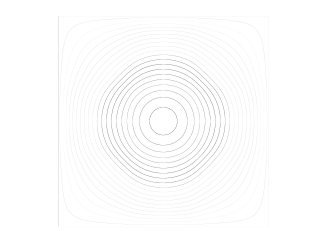
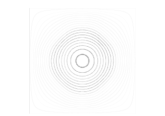
Figure 9. Left: data $u_{0}$ using fitted source term. Right: data $u_{0}$ using unfitted source term.

Figure 10. Convergence plot of the $L^{2}$-norm error of the reconstruction. Circle markers denote stabilized formulation and square markers unstabilized. Left: unperturbed data. Right: perturbed data. Dotted line is $h^{\frac{1}{2}}$ and same in both graphics. Filled line in right plot is $0.05h^{-1}$

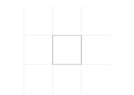
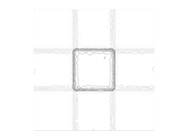
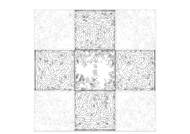
Figure 11. Contout lines of exact and reconstructed source terms. Left: exact source term. Middle: reconstructed source term using stabilization, unperturbed data. Right: unstabilized reconstruction, unperturbed data.

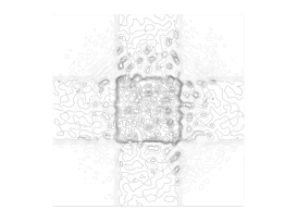
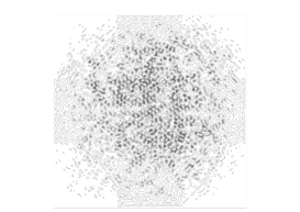
Figure 12. Left: reconstructed source term using stabilization, perturbed data. Right: unstabilized reconstruction, perturbed data.

References

- [1] G. Alessandrini, L. Rondi, E. Rosset, and S. Vessella. The stability for the Cauchy problem for elliptic equations. Inverse Problems, 25(12):123004, 47, 2009.
- [2] R. Becker, H. Kapp, and R. Rannacher. Adaptive finite element methods for optimal control of partial differential equations: basic concept. SIAM J. Control Optim., 39(1):113–132 (electronic), 2000.
- [3] E. Burman. Stabilised finite element methods for ill-posed problems with conditional stability. In LMS Proceedings. ”Building bridges: connections and challenges in modern approaches to numerical partial differential equations” 2014. Springer.
- [4] E. Burman. Stabilized finite element methods for nonsymmetric, noncoercive, and ill-posed problems. Part I: Elliptic equations. SIAM J. Sci. Comput., 35(6):A2752–A2780, 2013.
- [5] E. Burman. Error estimates for stabilized finite element methods applied to ill-posed problems. C. R. Math. Acad. Sci. Paris, 352(7-8):655–659, 2014.
- [6] E. Burman and A. Ern. Continuous interior penalty -finite element methods for advection and advection-diffusion equations. Math. Comp., 76(259):1119–1140 (electronic), 2007.
- [7] E. Burman and P. Hansbo. Edge stabilization for the generalized Stokes problem: a continuous interior penalty method. Comput. Methods Appl. Mech. Engrg., 195(19-22):2393–2410, 2006.
- [8] E. Burman, P. Hansbo, and M. G. Larson. A stabilized cut finite element method for partial differential equations on surfaces: the Laplace-Beltrami operator. Comput. Methods Appl. Mech. Engrg., 285:188–207, 2015.
- [9] A. Ern and J.-L. Guermond. Theory and practice of finite elements, volume 159 of Applied Mathematical Sciences. Springer-Verlag, New York, 2004.
- [10] D. F. Griffiths and J. M. Sanz-Serna. On the scope of the method of modified equations. SIAM J. Sci. Statist. Comput., 7(3):994–1008, 1986.
- [11] K. Ito and B. Jin. Inverse problems: Tikhonov theory and algorithms, volume 22 of Series on Applied Mathematics. World Scientific Publishing Co. Pte. Ltd., Hackensack, NJ, 2015.