Extreme dissipation event due to plume collision in a turbulent convection cell

Abstract

An extreme dissipation event in the bulk of a closed three-dimensional turbulent convection cell is found to be correlated with a strong reduction of the large-scale circulation flow in the system that happens at the same time as a plume emission event from the bottom plate. The reduction in the large-scale circulation opens the possibility for a nearly frontal collision of down- and upwelling plumes and the generation of a high-amplitude thermal dissipation layer in the bulk. This collision is locally connected to a subsequent high-amplitude energy dissipation event in the form of a strong shear layer. Our analysis illustrates the impact of transitions in the large-scale structures on extreme events at the smallest scales of the turbulence, a direct link that is observed in a flow with boundary layers. We also show that detection of extreme dissipation events which determine the far-tail statistics of the dissipation fields in the bulk requires long-time integrations of the equations of motion over at least hundred convective time units.

I Introduction

The highly nonlinear dynamics of fully developed turbulence generates high-amplitude fluctuations of the flow fields and their spatial derivatives. For the latter, amplitudes can exceed the statistical mean values by several orders of magnitude Yeung2015 . From a statistical point of view, extreme events correspond to amplitudes in the far tail of the probability density function of the considered field. Although the events are typically rare, they can appear much more frequently than for a Gaussian distributed field – a manifestation of (small-scale) intermittency in turbulence Frisch1994 ; Ishihara2009 . From a mathematical perspective, these high-amplitude events are solutions of the underlying dynamical equations which display a very rapid temporal variation with respect to a norm defined for the whole fluid volume Doering2009 . Typical quantities which can be probed are the vorticity or (local) enstrophy Lu2008 ; Donzis2010 , local strain Schumacher2010 or the magnitude of temperature, and passive scalar derivatives Kushnir2006 . Numerical studies of extreme events in turbulence have been performed in cubes with periodic boundaries in all three space dimensions Boratav1994 ; Donzis2010 . With increasing Reynolds number these extreme events in box turbulence are concentrated in ever finer filaments or layers Yeung2015 .

Alternatively, extreme dissipation events can be connected to flow structures in wall-bounded flows that have a large spatial coherence and exist longer than the typical eddies or plumes. Such dissipation events are observed for example in connection with ramp-cliff structures of the temperature Corrsin1962 ; Antonia1979 , with superstructures of the velocity Marusic2010 in atmospheric boundary layers, or with very-large scale motion in pipe flows Hellstroem2015 . High-dissipation events are then detected inside the container as well as at the edge of the boundary layers.

In this work, we demonstrate a direct dynamical link between a transition of the large-scale turbulent fields and the rare high-amplitude events of the spatial derivatives which are sampled at the smallest scales of the turbulent flow far away from the boundary layers. The system is a three-dimensional turbulent Rayleigh-Bénard convection (RBC) flow in a closed cylindrical cell. We show how the formation of a rare high-amplitude dissipation rate event in the bulk of the convection cell can be traced back to a plume emission from the bottom plate coinciding with a strong fluctuation of the large-scale circulation which exists in closed turbulent flows Ahlers2009 ; Chilla2012 . In the large-scale fluctuation event, the large-scale circulation (LSC) roll is significantly weakened and re-oriented afterwards. In the absence of the large-scale ordering circulation (which would sweep the plumes along with it), a collision between a hot upwelling and cold downwelling plume is triggered which generates strong local gradients. Such extreme dissipation events are very rare in the bulk since most of the viscous and thermal dissipation is inside the boundary layers at the top and bottom plates. This has been shown in several direct numerical simulations (DNS) of convection Emran2008 ; Kaczorowski2013 ; Scheel2013 . In our five high-resolution spectral element simulations at different Rayleigh and Prandtl numbers, we monitored the fourth-order moments of the thermal and kinetic energy dissipation rates in the bulk of the cell far away from the boundary layers. After finding one data point in one run which was much larger than the rest, we reran this full simulation twice in the interval around this extreme event at a monitoring frequency five and fifty times higher in order to analyze the dynamics in detail. Our detected rare event reveals a direct connection between a strong large-scale fluctuation of the velocity and a small-scale extreme dissipation (i.e. velocity derivative) event, thus bridging the whole cascade range of the turbulent flow.

II Numerical model

We solve the three-dimensional Boussinesq equations for turbulent RBC in a cylindrical cell of height $H$ and diameter $d$. The equations for the velocity field $u_{i}(x_{j},t)$ and the temperature field $T(x_{j},t)$ are given by

$$\partial_{i}u_{i} =0\,,$$ (1)

$$\partial_{t}u_{i}+u_{j}\partial_{j}u_{i} =-\partial_{i}p+\nu\partial_{j}^{2}u_{i}+g\alpha(T-T_{0})\delta_{iz}\,,$$ (2)

$$\partial_{t}T+u_{j}\partial_{j}T =\kappa\partial_{j}^{2}T\,,$$ (3)

with $i,j=x,y,z$ and the Einstein summation convention is used. The kinematic pressure field is denoted by $p(x_{j},t)$ and the reference temperature by $T_{0}$. The aspect ratio of the convection cell is $\Gamma=d/H=1$ with $x,y\in[-0.5,0.5]$ and $z\in[0,1]$. The Prandtl number which relates the kinematic viscosity $\nu$ and thermal diffusivity $\kappa$ is given by

$$Pr=\frac{\nu}{\kappa}\,.$$ (4)

The Rayleigh number is given by

$$Ra=\frac{g\alpha\Delta TH^{3}}{\nu\kappa}\,.$$ (5)

Here, the variables $g$ and $\alpha$ denote the acceleration due to gravity and the thermal expansion coefficient, respectively. The temperature difference between the bottom and top plates is $\Delta T$. In a dimensionless form all length scales are expressed in units of $H$, all velocities in units of the free-fall velocity $U_{f}=\sqrt{g\alpha\Delta TH}$ and all temperatures in units of $\Delta T$. Times are measured in units of the convective time unit, the free fall time $T_{f}=H/U_{f}$.

We apply a spectral element method in the present direct numerical simulations (DNS) in order to resolve the gradients of velocity and temperature accurately bib:nek5000 . More details on the numerical scheme and the appropriate grid resolutions can be found in Ref. Scheel2013 , and resolution of higher-order moments of the dissipation rates in Schumacher2014 . No-slip boundary conditions are applied for the velocity at all the walls. The top and bottom walls are isothermal and the side wall is thermally insulated.

The cylindrical convection cell is covered by $N_{e}$ spectral elements. On each element all turbulent fields are expanded by $N$th–order Lagrangian interpolation polynomials with respect to each spatial direction. Table 1 summarizes our highest Rayleigh number runs on massively parallel supercomputer simulations which have been carried out on up to 262144 MPI tasks. In the course of these production runs we conducted an analysis in which we searched for extreme dissipation events by means of the fourth-order moments obtained in an inner volume of the closed cylindrical cell.

The sequence around the extreme dissipation event was rerun twice to generate a fine sequence of one hundred snapshots with a separation of 0.143 free fall times $T_{f}$ and then a very fine sequence of five hundred snapshots with a separation of 0.029 $T_{f}$.

Run	$Ra$	$Pr$	$N_{e}$	$N$
1	$10^{8}$	0.7	256,000	11
2	$10^{9}$	0.7	875,520	11
3	$10^{10}$	0.7	2,374,400	11
4	$10^{7}$	0.021	875,520	11
5	$10^{8}$	0.021	2,374,400	13

Table 1: Parameters of the different spectral element simulations. We show the Rayleigh number $Ra$, the Prandtl number $Pr$, the total number of spectral elements $N_{e}$, and the polynomial order $N$ of the Lagrangian interpolation polynomials in each of the three space directions.

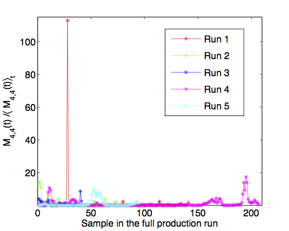
Figure 1: (Color online) Appearance of extreme thermal dissipation events in the bulk for five simulation runs which are listed in Table 1. The normalized fourth-order thermal dissipation rate moments $M_{4,4}(t)/\langle M_{4,4}(t)\rangle_{t}$ are shown versus the number of statistically independent samples saved in the simulation runs in subvolume $V_{4}$ which is approximately $V_{0}/5$.

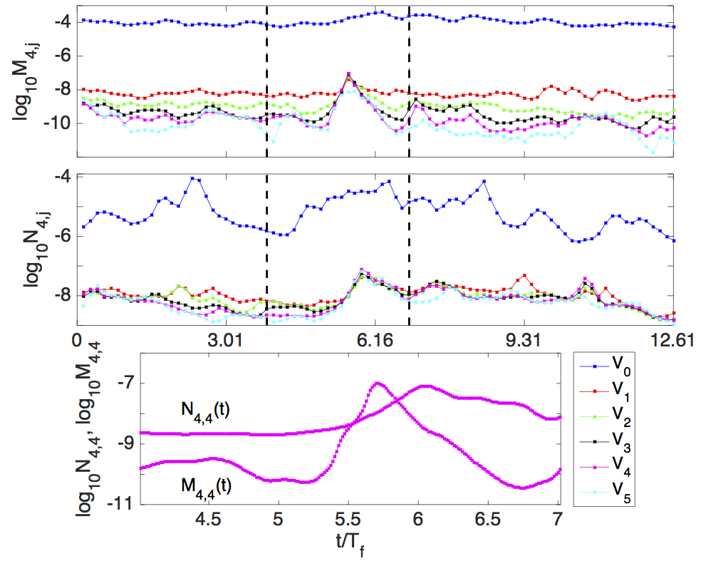
Figure 2: (Color online) Monitoring of the evolution of the extreme dissipation event in the bulk by means of the fourth moments of the thermal dissipation, $M_{4,j}$, (top panel) and kinetic energy dissipation, $N_{4,j}$, (mid panel). We display the moments in six different subvolumes $V_{1}\dots V_{5}$ and the whole cell $V_{0}$. The vicinity of the extreme event is marked by the vertical dashed lines and replotted in the bottom panel. These data are taken from the run with the finest temporal resolution.

Figure 3: (Color online) Five hundred individual probability density functions (PDFs) of the thermal dissipation rate $\epsilon_{T}$ in the left column and of the kinetic energy dissipation rate $\epsilon$ in the right column which are obtained from the run with the very fine time resolution. Data are for run 1. The insets replot data from the bottom panel of figure 2. The data in the vicinity of the local maxima are always highlighted as dark curves.

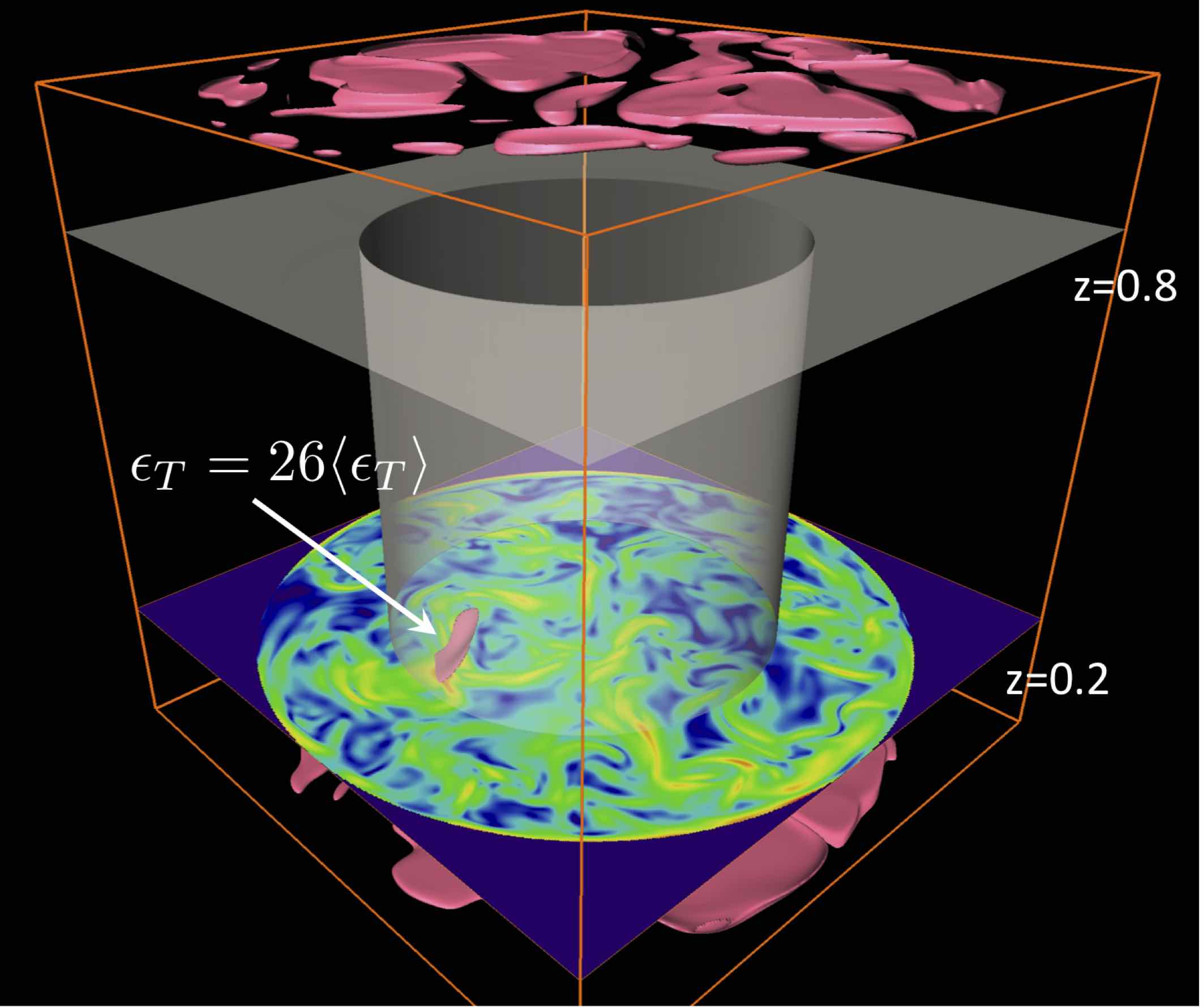
Figure 4: (Color online) Extreme thermal dissipation event in the bulk at time $T_{\ast}=5.73$. Combined plot of thermal dissipation rate (isosurfaces at $26\langle\epsilon_{T}\rangle_{V_{0},t}$) and kinetic energy dissipation rate (horizontal contour slice) on a logarithmic scale. Contour slice levels are from blue ($\log_{10}\epsilon\leq-4$) to red ($0.9\leq\log_{10}\epsilon)$. The inner cylinder stands for subvolume $V_{4}$ with $r\leq 0.3$ and $0.2\leq z\leq 0.8$.

III Results

III.1 Detection by fourth-order moments

The starting point of the analysis is the time evolution of the fourth-order moments of the kinetic energy dissipation rate,

$$\epsilon(x,y,z,t)=2\nu S_{ij}S_{ji}\,,$$ (6)

with $S_{ij}=(\partial_{i}u_{j}+\partial_{j}u_{i})/2$, and the thermal dissipation rate,

$$\epsilon_{T}(x,y,z,t)=\kappa G_{i}^{2}\,,$$ (7)

with $G_{i}=\partial_{i}T$. The Rayleigh-Bénard flow in the cylindrical cell obeys statistical homogeneity in the azimuthal direction only. All statistics will therefore depend on the size of the sample volume. We have monitored the moments in six successively smaller cylindrical subvolumes which are nested in each other. We define $r_{0}=0.5>r_{1}=0.45>\dots>r_{5}=0.25$ and $h_{0}=1>h_{1}>\dots>h_{5}=0.5$ and $V_{j}=\{(r,\phi,z)\,|\,r\leq r_{j}\;,(1-h_{j})/2\leq z\leq(1+h_{j})/2\}$ with $j=0\dots 5$. The volume $V_{0}$ is the full cell. Fourth-order moments of both dissipation rates are given by

$$M_{4,j}(t)=\langle\epsilon_{T}^{4}\rangle_{V_{j}}\quad\mbox{and}\quad N_{4,j}(t)=\langle\epsilon^{4}\rangle_{V_{j}}\,.$$ (8)

In figure 1 the normalized moments of the thermal dissipation rate are shown for five different runs which are obtained at the highest Rayleigh numbers and two different Prandtl numbers (see table 1). In the primary production runs we analysed the kinetic energy and thermal dissipation rate in the subvolume $V_{4}$ that is sufficiently far away from all boundaries. Since the simulation runs have a different number of time step widths and a different number of data output steps, the moments are shown versus the number of samples. It is clearly visible that in all runs the volume averages can go far beyond the means at certain times. However, the strongest outlier is observed for run 1 at $Ra=10^{8}$ and $Pr=0.7$. Therefore, the discussion in this work is dedicated to run 1.

In figure 2 we display $M_{4,j}(t)$ (top panel) and $N_{4,j}(t)$ (mid panel) on a semi-logarithmic plot for run 1. Data are obtained over a time interval with an output of one hundred snapshots separated by 0.143 free fall times units (see top and mid panels of the figure). $M_{4,0}(t)$ remains nearly unchanged and $N_{4,0}(t)$ fluctuates more strongly, but there is no large event that stands out. The reason is that a major part of both the thermal variance and of the kinetic energy is dissipated in the boundary layers of the temperature and velocity fields close to the walls, respectively Emran2008 ; Kaczorowski2013 ; Scheel2013 . Only in the successively smaller subvolumes $V_{j}$, that are nested increasingly deeper in the bulk, is the extreme bulk dissipation event detected by the corresponding fourth order moment. It is seen that $M_{4,4}(t)$ grows by three orders of magnitude within $T_{f}/2$. The bottom panel of figure 2 shows that a local, but less strong maximum of $N_{4,4}(t)$ occurs approximately $T_{f}/2$ after the peak in $M_{4,4}$.

The significance of this event for the small-scale statistics of the temperature and velocity derivatives in the bulk region is demonstrated in figure 3. In both cases the fattest tail corresponds with this high-amplitude event as seen in the bottom panels of figure 3. We display five hundred individual probability density functions (PDFs), each taken at one instant in time. These data have been obtained in a repetition run at the highest temporal resolution in order to resolve the event better. The vicinity of the high-dissipation event is colored differently in both dissipation rates. It is also seen that the high-dissipation bulk event does not contribute significantly to the far tails of the PDFs when averaged over the whole convection cell including all boundary layers. The resulting extension of the far tail of the time-averaged PDFs in the bulk was already shown in ref. Scheel2013 .

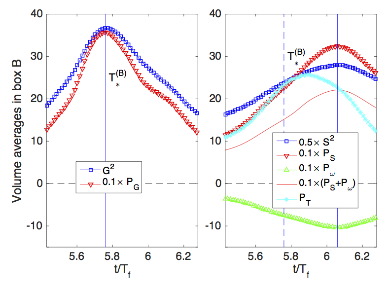
Figure 5: (Color online) Time evolution of production terms and magnitudes in the course of the extreme event. All quantities are now volume averages taken for box ${\cal B}$. The maximum of $G^{2}$ is at $T_{\ast}^{({\cal B})}=5.759$ and is slightly shifted with respect to $T_{*}$ in $V_{4}$ because $V_{4}\gg{\cal B}$ and the temporal resolution is finer. Left: temperature gradient square and production term $P_{G}$ (see eq. (9)). Right: local strain and production terms $P_{S}$, $P_{\omega}$ as well as $P_{T}$ (see eq. (10)). The peaks of $G^{2}$ (left) and $S^{2}$ (right) are indicated by solid vertical lines. The dashed vertical line in the right panel is the maximum of $G^{2}$. Terms are partly rescaled as indicated in the legend.

III.2 Link between high-amplitude thermal and kinetic energy dissipation events

Figure 4 shows isosurfaces of the thermal dissipation rate at $\epsilon_{T}=26\langle\epsilon_{T}\rangle_{V_{0},t}$ which are mostly found close to the top and bottom plates. The same holds for kinetic energy dissipation, but is not shown. It is the high-thermal-dissipation sheet at $T_{\ast}=5.73$ which is mostly inside $V_{4}$ that contributes to the local maxima of $M_{4,j}(t)$ for $j>0$ in figure 2. It can be also seen that the local maximum of $\epsilon_{T}(x,y,z,t)$ coincides with a local maximum of $\epsilon(x,y,z,t)$. The temperature front generates a strong shear layer which is manifest as a delayed high-amplitude energy dissipation event.

We refined the analysis, both in space and time. We zoom into the small box ${\cal B}=\{(x,y,z)\in[-0.11,-0.05]\times[-0.34,-0.14]\times[0.15,0.33]\}$ that encloses the high-amplitude thermal dissipation layer. The balance equation for the square of the magnitude of $G_{i}$ is given by Pumir1994 ; Brethouwer2003

$$\frac{\mbox{d}G^{2}}{\mbox{d}t}=-2G_{i}S_{ij}G_{j}+2\kappa G_{i}\frac{\partial^{2}G_{i}}{\partial x_{j}^{2}}\,.$$ (9)

The first term on the right hand side is the gradient production term, $P_{G}$. Local shear strength is measured by the square of the magnitude of the rate of strain tensor $S^{2}=S_{ij}S_{ji}$. The balance equation for $S^{2}$ (see also Holzner2008 ) has to be extended by a temperature production term and is given by

$$\frac{\mbox{d}S^{2}}{\mbox{d}t}= -2S_{ij}S_{jk}S_{ki}-\frac{1}{2}\omega_{i}S_{ij}\omega_{j}-2S_{ij}\frac{\partial^{2}p}{\partial x_{i}\partial x_{j}}$$

$$+2\nu S_{ij}\frac{\partial^{2}S_{ij}}{\partial x_{k}^{2}}+2g\alpha S_{zi}G_{i}\,.$$ (10)

We have three production terms: strain production (1st, $P_{S}$), enstrophy consumption (2nd, $P_{\omega}$) and production due to coupling to the temperature gradient (last, $P_{T}$).

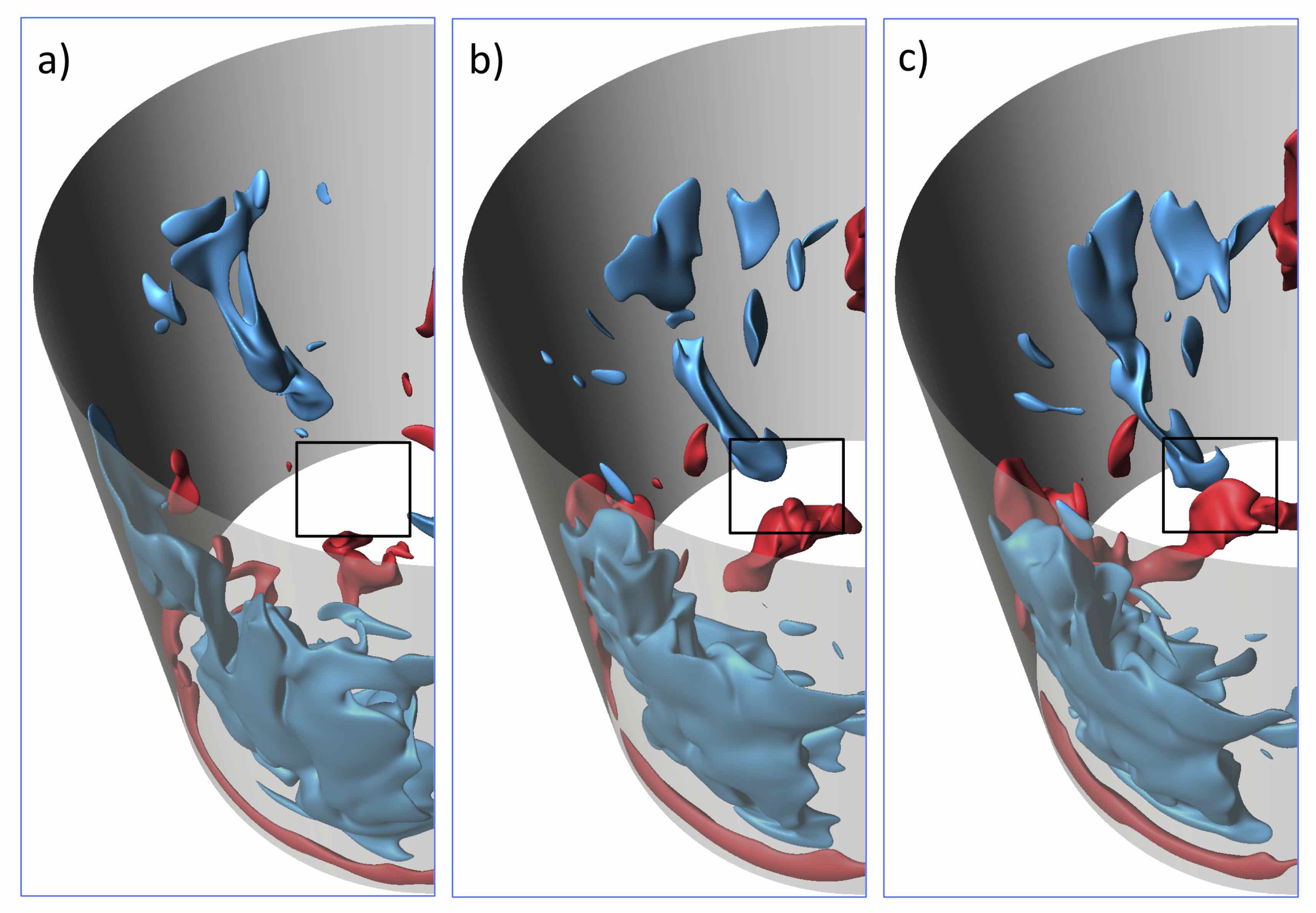
Figure 6: (Color online) Isocontour plot of the vertical convective current for times: (a) $T_{\ast}-1.146$, (b) $T_{\ast}-0.296$ and (c) $T_{\ast}$. Blue is for downwelling at $\sqrt{RaPr}\,u_{z}T=-900$, red for upwelling plumes at $\sqrt{RaPr}\,u_{z}T=1000$. The collision region is indicated by a box.

Figure 5 displays the time evolution of volume averages over ${\cal B}$ for both gradient magnitudes and the corresponding production terms in eqns. (9) and (10), respectively. The maximum of $G^{2}$ coincides with the one of $P_{G}$ (see left panel). The same holds for the maximum of $S^{2}$ and the ones of $P_{S}$ and $\left|P_{\omega}\right|$, respectively (right panel). We also confirm that $\max\langle S^{2}\rangle_{\cal B}$ lags behind $\max\langle G^{2}\rangle_{\cal B}$ (see also figure 2), a result which is also robust for different sizes of ${\cal B}$. The time of maximum production by $P_{T}$, falls right between those for $P_{G}$ and $P_{S}+P_{\omega}$. This shows that the temperature gradient occurs first, followed by strong shear generation since the colliding fluid masses have to move around each other.

III.3 Formation of colliding plumes

How is the high-amplitude thermal dissipation layer formed? Figure 6 plots isosurfaces of the vertical component of the convective heat current vector $j^{c}_{z}=\sqrt{RaPr}\,u_{z}T$ at three instants. Since $0\leq T\leq 1$, a negative isolevel of $j_{z}^{c}$ corresponds to a downwelling and a positive one to an upwelling plume. The box in the panels indicates the collision point of two plumes in the bulk at time $T_{\ast}$. This collision is caused by the large hot plume from the bottom and a second extended cold plume that falls down at the side wall and turns into the bulk. The high-amplitude thermal dissipation layer is formed at the collision site. The event is comparable with rapid growth events of enstrophy in box turbulence Lu2008 . There colliding vortex rings maximized enstrophy growth. Our nearly frontal plume collision can be considered thus a rare event and appears in three-dimensional convection flow much less frequently than in two-dimensional ones Chandra2013 .

First we will investigate the rising hot plume. Figure 7 displays contours of $\partial T/\partial z$ at the bottom plate. Local maxima are indicators for rising plumes Bandaru2015 . On top of contours we plot field lines of the skin friction field which is given by $\partial_{i}u_{j}|_{z=0}=(\partial_{z}u_{x},\partial_{z}u_{y})$ Chong2012 . Locally downwelling fluid impacts the bottom plate and generates unstable node points (UN) of the skin friction field. Skin friction lines, which arise from these nodes, form a strong front which starts to form in panel (a) and is moved “upward” in panel (b) of figure 7. Saddle points (SP) or stable nodes (SN) are formed between the unstable nodes. The unstable manifold of a saddle Bandaru2015 or a sequence of stable nodes, as being the case here, are the preferred sites of plume formation. It is the persistence and convergence of these critical points for a certain time span which causes the rise of a large plume from the bottom just before $T_{\ast}$, that then collides with the downwelling cold plume at $T_{\ast}$.

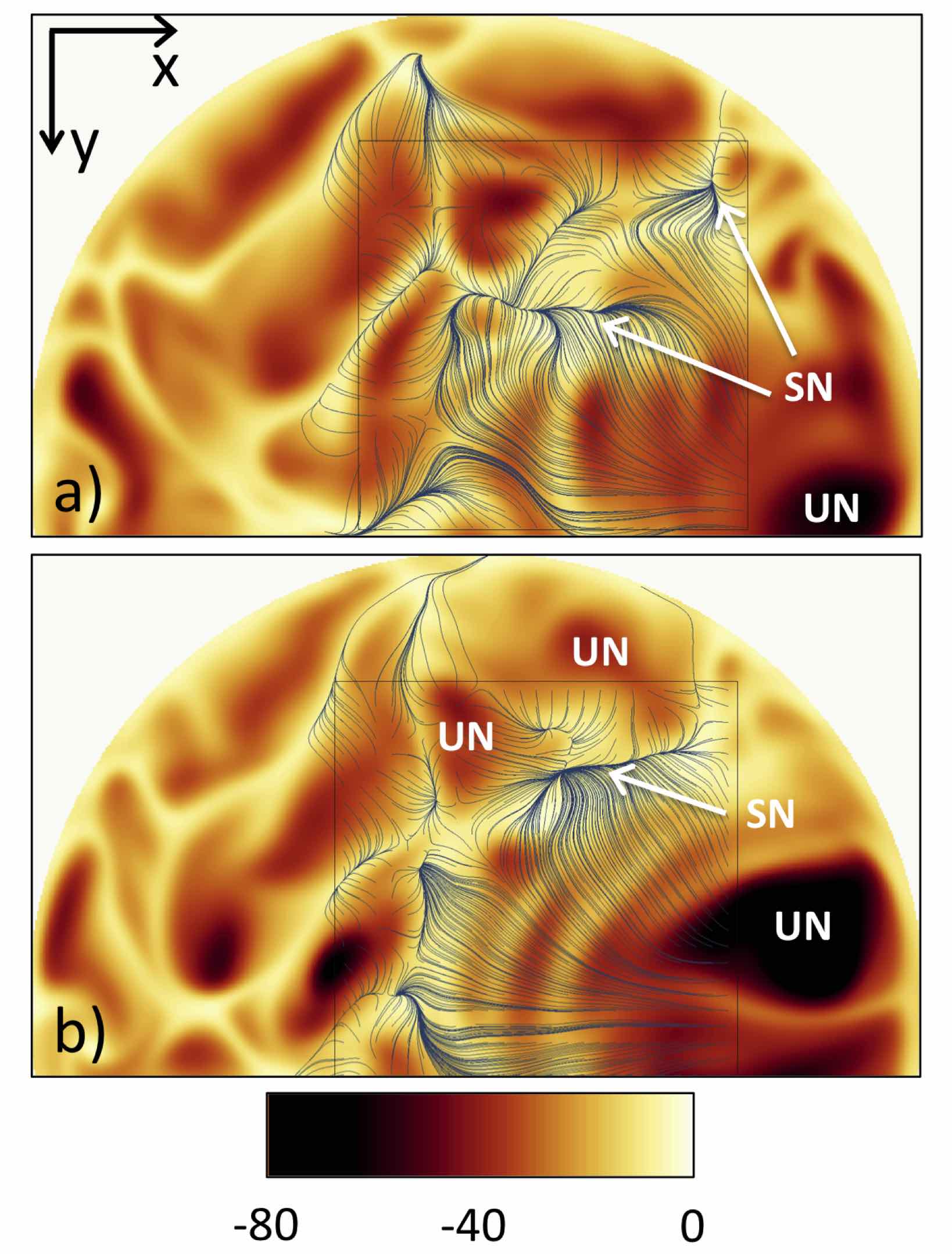
Figure 7: (Color online) Strong plume formation at the bottom plate. Contour plots of $\partial T/\partial z$ at $z=0$ are shown together with field lines of the skin friction field $(\partial u_{x}/\partial z,\partial u_{y}/\partial z)$. Times are $T_{\ast}-1.146$ for (a) and $T_{\ast}-0.296$ for (b). For better visibility, we seed the skin friction lines only in a square box around the rising plume. Stable nodes (SN) and unstable nodes (UN) are indicated.

III.4 Plume collision due to transition of large-scale flow

This raises the last question, namely does a change in the large-scale dynamics enable such a rare plume collision event? It is well-known that in closed convection cells a large-scale circulation (LSC) exists Ahlers2009 ; Chilla2012 . In cells with $\Gamma=1$, the LSC consists of one big roll which forces the plumes to move along the top or bottom plate, and then to rise dominantly on one side of the cell and to fall down on the other side. This ordering influence stops when the large-scale circulation decelerates strongly and becomes re-oriented. Such events have been studied statistically in experiments Sreenivasan2002 ; Brown2006 ; Xi2007 , numerically in two-dimensional Chandra2013 ; Petschel2011 ; Poel2012 or three-dimensional Mishra2011 convection as well as in low-dimensional models Brown2008 .

We quantified the large-scale dynamics by taking a spatial average with respect to the radial and vertical coordinates. We define

$$\overline{u_{z}T}(\phi,t)=\frac{1}{{\cal V}_{r}}\int_{r_{1}}^{r_{2}}\int_{z_{1}}^{z_{2}}u_{z}T(r,\phi,z,t)\,rdrdz\,,$$ (11)

with ${\cal V}_{r}=\pi(r_{2}^{2}-r_{1}^{2})(z_{2}-z_{1})$. The complex three-dimensional structure of the up- and downwelling convective currents in the closed cell is thus reduced to a one-dimensional signal. The locally averaged convective current $\overline{u_{z}T}(\phi,t)$ is expanded in a Fourier series for each instant

$$\overline{u_{z}T}(\phi,t)=\sum_{m=1}^{N}a_{m}(t)\cos(m\phi+\gamma_{m}(t))\,.$$ (12)

Figure 8 displays the amplitude of the first three modes, $a_{1}(t)$ to $a_{3}(t)$. We have chosen different vertical intervals $[z_{1},z_{2}]$, in the upper and lower sections of the cell as well as in the center. At the beginning of the time window, we find $a_{1}>a_{2}>a_{3}$ in all sections of cell. This indicates that a one-roll circulation pattern dominates the LSC as is supported by the isocontours in Figure 8(d). In Figures 8(a)–(c), $a_{1}$ steadily decreases towards $t=T_{\ast}$ with $T_{\ast}$ being the time of the extreme dissipation event. The ratio of the Fourier coefficients is changed to $a_{1}\sim a_{3}>a_{2}$ for the lower section of the cell (see Figure 8(c)), while in the mid and upper sections (see Figures 8(a,b)), $a_{1}>a_{3}>a_{2}$ is observed. The growth of the $m=3$ mode demonstrates that up- and downwelling convective currents are found now close to each other, in particular in the lower section of the cell, as can be seen by the isocontours in Figure 8(e). For $t>T_{\ast}$, we observe a re-establishment of the one-roll pattern, as supported by Figure 8(f). The whole process proceeds within $10T_{f}$. Also plotted in Figures 8(d)–(f) are the isocontours for large $\epsilon_{T}$, which always are located near the bottom and top plates. However, in Figure 8e, one sees a region of large $\epsilon_{T}$ in between the upwelling hot and downwelling cold plumes as they collide, consistent with the increase in $\epsilon_{T}$ in the bulk seen in Figure 2.

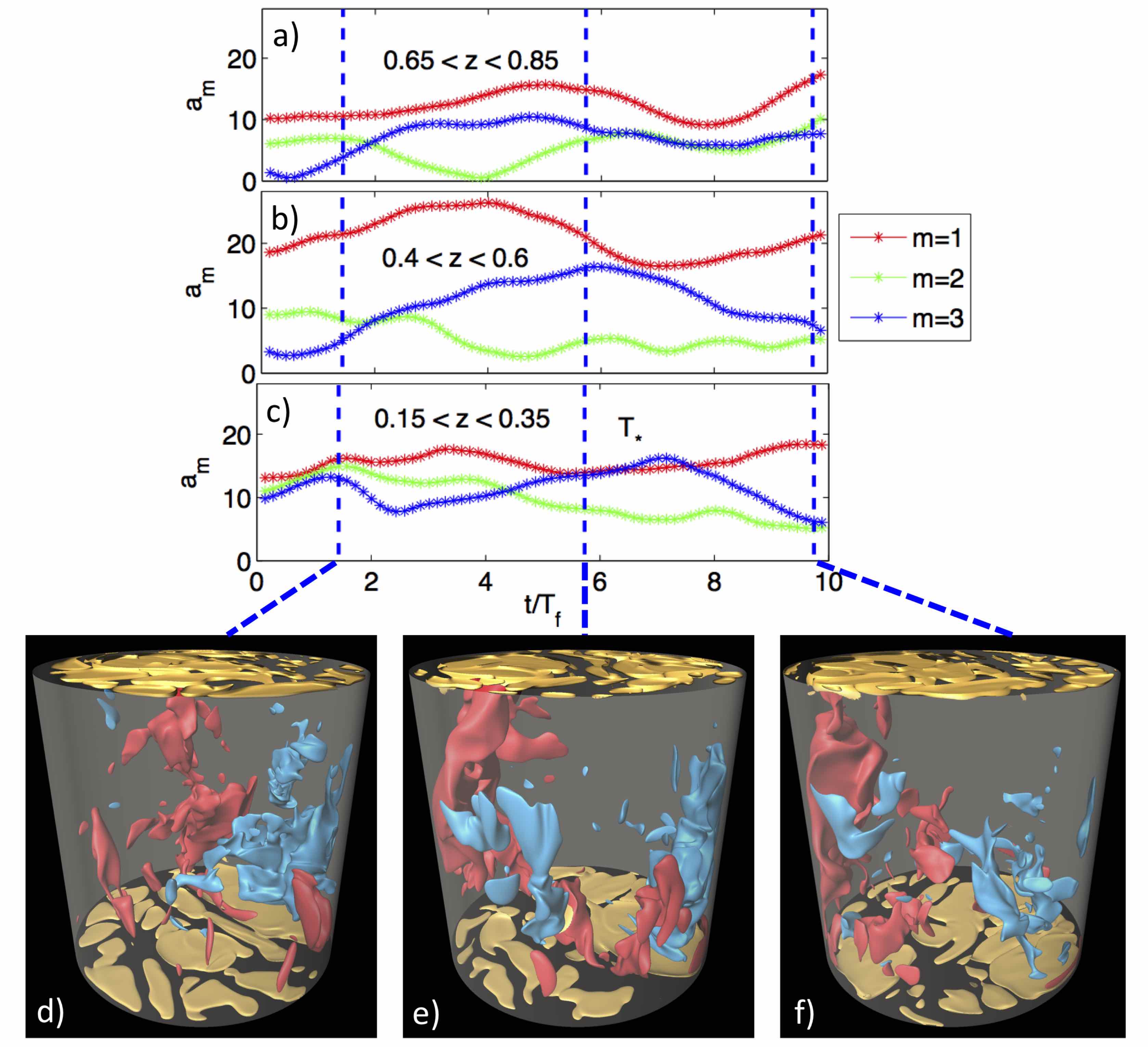
Figure 8: (Color online) Time evolution of the three largest Fourier mode amplitudes obtained for $\overline{u_{z}T}(\phi,t)$. (a) $z_{1}=0.65<z<z_{2}=0.85$. (b) $0.4<z<0.6$. (c) $0.15<z<0.35$. Points $0.4<r<0.48$ were taken in radial direction. At the bottom we add three snapshots of the convective current $\sqrt{RaPr}\,u_{z}T$ (blue for level of -900 and red for level of 1100) together with isocontours of $\epsilon_{T}=0.1\approx 26\langle\epsilon_{T}\rangle_{V_{0},t}$. (d) $t=1.43$. (e) $t=T_{\ast}=5.73$. (f) $t=9.74$.

IV Summary

We have connected a far-tail, extreme dissipation event at the small scales in the bulk of a three-dimensional Rayleigh-Bénard convection flow in a closed cell to a reduction event in the LSC accompanied by a plume emission from the bottom boundary layer. Such an event is very rare. In five different simulations spanning a range of $Ra$ and $Pr$ over long evolution times it was the only very high dissipation event in the bulk away from boundary layers as shown in figure 1.

The detection was possible by monitoring the well-resolved fourth-order dissipation moments in the bulk of the cell during the simulations. We also have showed how a transition of the large-scale flow structures in the cell can impact the dynamics at the smallest scales, the scales across which the steepest gradients are formed. The two events are thus directly linked and bridge the whole scale range of the turbulent cascade. The large-scale coherent fluid motion is established here due to the presence of walls which enclose the convection cell. It can be expected that it would be absent in box turbulence with periodic boundary conditions.

How frequently does such a high-dissipation event appear? If one takes a typical far-tail amplitude of the PDF of $\epsilon_{T}$ (see lower left panel of figure 3) of $p(\epsilon_{T})\sim 10^{-6}$ and multiplies it with the binwidth $\Delta\epsilon_{T}=0.0004$, one gets an estimate of the probability of the appearance of a high-thermal-dissipation event in the bulk of $w\approx p(\epsilon_{T})\Delta\epsilon_{T}\approx 4\times 10^{-10}$, i.e., one out of 2.5 billion data points. The bulk volume $V_{4}$ contains about a fifth of the total cell volume and about 10 per cent of the total number of mesh cells which translates to roughly 40 million cells for $V_{4}$. That means that one picks such high-dissipation events every 60 to 70 $T_{f}$ if one continues with the same sampling frequency as in the original production run. Our total integration time for run 1 was 104 $T_{f}$. Consequently, if one wants to have a complete picture of the small-scale statistics of a wall-bounded turbulent flow then these events have to be incorporated. As our estimate shows, this requires very long-time integrations of the fully resolved Boussinesq equations which becomes increasingly expensive as the Rayleigh number grows or the Prandtl number decreases.

- (1) P. K. Yeung, X. M. Zhai and K. R. Sreenivasan, Proc. Natl. Acad. Sci. USA 112, 12633 (2015).
- (2) U. Frisch, Turbulence – The Legacy of A. N. Kolmogorov. Cambridge University Press, Cambridge, 1994.
- (3) T. Ishihara, T. Gotoh and Y. Kaneda, Annu. Rev. Fluid Mech. 41, 165 (2009).
- (4) C. R. Doering, Annu. Rev. Fluid Mech. 41, 109 (2009).
- (5) L. Lu and C. R. Doering, Indiana Univ. Math. J. 57, 2693 (2008).
- (6) D. A. Donzis and K. R. Sreenivasan, J. Fluid Mech. 647, 13 (2010).
- (7) J. Schumacher, B. Eckhardt and C. R. Doering, Phys. Lett. A 374, 861 (2010).
- (8) D. Kushnir, J. Schumacher and A. Brandt, Phys. Rev. Lett. 97, 124502 (2006).
- (9) O. N. Boratav and R. B. Pelz, Phys. Fluids 6, 2757 (1994).
- (10) S. Corrsin, Phys. Fluids 5, 1301 (1962).
- (11) R. A. Antonia, A. J. Chambers, C. A. Friehe, and C. W. van Atta, J. Atmos. Sci. 36, 99 (1979).
- (12) I. Marusic, R. Mathis and M. Hutchins, Science 329, 193 (2010).
- (13) L. H. O. Hellström, B. Ganapathisubramania and A. J. Smits, J. Fluid Mech. 779, 701 (2015).
- (14) G. Ahlers, S. Grossmann and D. Lohse, Rev. Mod. Phys. 81, 503 (2009).
- (15) F. Chillà and J. Schumacher, Eur. Phys. J. E 35, 58 (2012).
- (16) M. S. Emran and J. Schumacher, J. Fluid Mech. 611, 13 (2008).
- (17) M. Kaczorowski and K.-Q. Xia, J. Fluid Mech. 722, 596 (2013).
- (18) J. D. Scheel, M. S. Emran, and J. Schumacher, New J. Phys. 15, 113063 (2013).
- (19) http://nek5000.mcs.anl.gov
- (20) J. Schumacher, J. D. Scheel, D. Krasnov, D. A. Donzis, V. Yakhot and K. R. Sreenivasan, Proc. Natl. Acad. Sci. 111, 10961 (2014).
- (21) A. Pumir, Phys. Fluids 6, 2118 (1994).
- (22) G. Brethouwer, J. C. R. Hunt and F. T. M. Nieuwstadt, J. Fluid Mech. 474, 193 (2003).
- (23) M. Holzner, A. Liberzon, N. Nikitin, B. Lüthi, W. Kinzelbach and A. Tsinober, J. Fluid Mech. 598, 465 (2008).
- (24) M. Chandra and M. K. Verma, Phys. Rev. Lett. 110, 114503 (2013).
- (25) V. Bandaru, A. Kolchinskaya, K. Padberg-Gehle and J. Schumacher, Phys. Rev. 92, 043006 (2015).
- (26) M. S. Chong, J. P. Monty, C. Chin and I. Marusic, J. Turb. 13, N6 (2012).
- (27) K. R. Sreenivasan, A. Bershadskii and J. J. Niemela, Phys. Rev. E 65, 056306 (2002).
- (28) E. Brown and G. Ahlers, J. Fluid Mech. 568, 351 (2006).
- (29) H.-D. Xi and K.-Q. Xia, Phys. Rev. E 75, 066307 (2007).
- (30) K. Petschel, M. Wilczek, M. Breuer, R. Friedrich and U. Hansen, Phys. Rev. E 84, 026309 (2011).
- (31) E. van der Poel, R. A. J. M. Stevens, K. Sugiyama and D. Lohse, Phys. Fluids 24, 085104 (2012).
- (32) P. K. Mishra, A. K. De, M. K. Verma and V. Eswaran, J. Fluid Mech. 668, 480 (2011).
- (33) E. Brown and G. Ahlers, Phys. Fluids 20, 075101 (2008).