Kinetics of fragmentation and dissociation of two-strand protein filaments: coarse-grained simulations and experiments

Abstract

While a significant body of investigations have been focused on the process of protein self-assembly, much less is understood about the reverse process of a filament breaking due to thermal motion into smaller fragments, or depolymerization of subunits from the filament ends. Indirect evidence for actin and amyloid filament fragmentation has been reported, although the phenomenon has never been directly observed either experimentally or in simulations. Here we report the direct observation of filament depolymerization and breakup in a minimal, calibrated model of coarse-grained molecular simulation. We quantify the orders of magnitude by which the depolymerization rate from the filament ends $k_{\mathrm{off}}$ is larger than fragmentation rate $k_{-}$ and establish the law $k_{\mathrm{off}}/k_{-}=\exp[(\varepsilon_{\|}-\varepsilon_{\bot})/k_{\mathrm{B}}T]=\exp[0.5\varepsilon/k_{\mathrm{B}}T]$, which accounts for the topology and energy of bonds holding the filament together. This mechanism and the order-of-magnitude predictions are well supported by direct experimental measurements of depolymerization of insulin amyloid filaments.

I Introduction

The strong directionality of non-covalent physical bonds between proteins underlies their strong propensity to self-assemble into fibrils and filaments. Protein filaments are ubiquitous in biology, appearing individually, in bundles, or in randomly crosslinked networks. They facilitate the propulsion of bacteria and extension in lamellipodia, they control the mechanical strength of the cytoskeleton and the bending stiffness in axons, they allow positional control of organelles and provide transport pathways all around the cell 1-Oosawa ; 2-Alberts . In a different context, the self-assembly of misfolded proteins into amyloid fibrils impairs physiological activity and is associated with a number of organic dysfunctions 3-Chiti ; 4-Chandler ; 5-Irback . In yet another context, filaments are artificially or spontaneously assembled to achieve a specific function in the material, such as directed conductivity, plasmonic resonances, or just the mechanical strength in a fibre composite, all with important technological applications. While a huge number of experimental and computational studies are available on the mechanism of self-assembly of proteins into filaments, the reverse process of filament breakup (fragmentation) remains poorly understood and controversial 6-Wegner ; 7-Wegner ; 8-Pollard ; 9-Erickson ; 10-Kinosian ; 11-Sept ; 12-Pollard ; 13-Fushiwara ; 14-Kuhn ; 15-Fass .

I.1 The two cases of actin filaments and amyloid fribrils

In the case of actin, the depolymerization rates were measured long ago by Pollard 8-Pollard , but no direct measurement of fragmentation is available: fragmentation rates are typically deduced from kinetic modelling assuming an equilibrium between fragmentation and filament-filament annealing 6-Wegner ; 7-Wegner ; 9-Erickson ; 11-Sept . For F-actin, both end-dissociation and fragmentation are influenced by chemical factors: F-actin is ADP-bound at the pointed end and in the inner filament, where fragmentation occurs, while it is mostly ATP-bound at the barbed end (with a smaller end-dissociation rate), especially in the treadmilling and fast polymerization regimes 2-Alberts . The ADP-complexation thus reduces the binding energy somewhat compared to ATP, resulting to higher rates for thermal escape of a subunit from the attractive potential well with its bonded subunits. As shown experimentally Vavylonis , and also by theoretical modelling Kolom-Biophys , growth rates and the critical concentration at the barbed end are intimately related to the cap structure and dynamics. However, these effects are less important for dissociation processes where only ADP is left inside actin monomers.

In the case of amyloid filaments, which have a similar multi-stranded structure but different protein-protein bonding, no data on end-dissociation is available while the rates of fragmentation are similarly deduced from kinetic modelling 16-Knowles ; 17-Adamcik . This gap in the current knowledge has important consequences: in the case of actin, it is fragmentation which sets both the lifetime of actin filaments (to ca. 500 s in vitro 2-Alberts ) and their plateau average length 9-Erickson , as well as secondary nucleation and rapid growth of amyloid fibrils (self-catalytic activity). The physics of fragmentation is crucial to explain the anomalously large length-diffusivities, the microscopic mechanism of severing in vivo, and to engineer the mechanical properties of artificial filaments for biotechnology. Also, little is known about the rates of end-dissociation in amyloids, while the fragmentation is estimated from the equilibrium kinetics balance, and the customary assumption is to take both rates equal 16-Knowles ; 20-Lee , which is an assumption very far from reality, as we will show below.

I.2 Simplified self-assembly framework

In a simplified framework that neglects the role of active oligomers and nuclei, the filament growth can be summarised by the reversible reaction: $A_{1}+A_{p}\rightleftharpoons A_{p+1}$, where the monomer subunit $A_{1}$ is added to a filament of $p$ units. For the forward reaction, it is accepted that association is dominated by the addition of a single subunit (elongation), while annealing (joining of two fragments) is much slower, because of the greater abundance of monomers with respect to active oligomers and the fast decay of filament mobility with its length 18-Kas . The subunit dissociation reaction from the end is known to be dominant in the case of actin 9-Erickson ; 15-Fass ; 19-Pollard , although the much slower fragmentation reaction is the one which controls the late-stage plateau in the growth.

Here we provide a minimal numerical model of break-up rates which attempts to bring together the essential features of both actin and amyloid filaments. Although more dynamic exchange processes (such as those described e.g. in Ref.Carulla ; Vestergaard ) are neglected in order to focus on the general mechanisms, the model predictions for the rates of fragmentation and dissociation are satisfactorily verified with new experiments for the case of amyloid-like insulin fibrils. Although we aim to provide the missing breakup mechanism for the specific case of amyloid-like filaments, our framework is general. By combining it with detailed atomistic approaches it will be useful for the control of biofilaments size in biotechnological applications (e.g. biomaterials for regenerative tissues, biofilms, etc).

II Results and Discussion

II.1 Coarse-grained numerical model

To model a protein filament we use a coarse-grained model where the protein monomers are treated as Brownian spherical particles of diameter $\sigma$ assembled into a two-stranded structure shown in fig. 1. This two-stranded topology (which includes the double-helix as one of its variants) is one of the most commonly observed structures for both F-actin and amyloid filaments. Each protein is interacting with two other proteins along the same chain (longitudinal bonds), and with a third protein on the second chain (transversal bond). The strength of the physical bonding is $\varepsilon_{\|}$ along the filament and $\varepsilon_{\bot}$ with the matching subunits in the parallel strings. This is clearly a minimal model which however allows us to capture the general features of two-strand filament breakup without the complications that lie in the peculiar chemistry of different proteins. Hence, it is hoped that the model predictions capture essential features that are common to both actin filaments and amyloid fibrils.

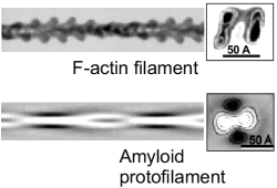
Figure 1: Images reconstructed from cryo-EM experiments on actin filaments and insulin amyloid protofilament, both showing a characteristic two-strand structure of protein subunits bonded by physical interactions. In F-actin, the growth occurs from the ATP-functionalized B-end and the dissociation from the P-end where the F-actin subunits contain ADP. In the case of amyloids, the growth and dissociation occur symmetrically from both ends.

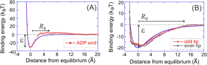
Figure 2: (A) The molecular-dynamics calculation of the effective binding potential of a single actin-ADP subunit and the remaining filament at the P-end. The plot shows the two key parameters: the cutoff distance $R_{c}$ and the potential depth $\varepsilon$, which is in good agreement with previous experimental estimates 9-Erickson . (B) A similar molecular-dynamics calculation of the effective binding potential for a dimer of A$\beta$-amyloids taken from Ref.25-Han . In both graphs the data points are fitted with the (12-6) Lennard-Jones potential, showing a good qualitative agreement (although with expected differences at the long-range attractive tail given the complex shape of the subunit): the depth of the binding well, typically on the order of 20-30$k_{\mathrm{B}}T$.

Interactions between two proteins are modelled as the sum of a non-covalent Lennard-Jones (LJ) interaction, and a bond-bending angular interaction. The LJ potential describes the short-range steric repulsion between two proteins, which co-exists with a central-force (London-van der Waals) attraction due to hydrogen bonds holding two $\beta$-sheets together (prevalent in amyloids) – or the hydrophobic interaction with a subunit perpendicular to the chain (dominant in F-actin), see fig. 2. The bond-bending term, instead, originates from the geometrical constraint imposed by the $\beta$-sheet connection or by other anisotropic steric interactions. In simple terms, when two planar surfaces ($\beta$-sheets) are connected by several springs (hydrogen bonds), any tangential displacement (orthogonal to the direction connecting the two centers of mass of the two proteins) costs a finite amount of energy, because of the rotational symmetry-breaking. The local bond-bending modulus $K$, in units of $k_{\mathrm{B}}T$, is directly related to the persistence length $l_{p}$ of the filament via the standard expression: $l_{p}=K\sigma/k_{\mathrm{B}}T$. In fig. 3 filaments with different values of bending stiffness $K$ are shown, to illustrate the effect $K$ has on the overall stiffness/flexibility of the filament.

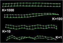
Figure 3: An illustration of the role of bending rigidity: instantaneous shapes of a coarse-grained two-stranded filament with increasing bending modulus $K$ (in units of $k_{\mathrm{B}}T$).

To calibrate our coarse-grained potential on realistic filaments, we can therefore use the experimentally known persistence length $l_{p}$ to guide our choice of $K$ in the simulations. For biological filaments the persistence length is long, though not infinite. While it can reach up to 1mm for microtubules, it is typically about 18$\mu$m $\approx$3600 subunits for F-actin 21-Gittes and 3$\mu$m $\approx$5000 subunits for amyloid-like insulin filaments 22-Knowles . These persistence lengths in our simulations can be reproduced using large values of bond-bending stiffness: $K\approx 10^{4}$ (in units of $k_{\mathrm{B}}T$). We have checked that our results for the breakup rate and fragment distributions did not vary when $K$ is in the range $10^{3}$-$10^{5}$.

II.2 Calibration of simulation parameters

Next, we consider the parameters which control the LJ interaction, namely the magnitude of binding energy $\varepsilon$ and the cut-off $R_{c}$. To calibrate these parameters, we first consider how they affect the breakup rates and fragment distributions. In our simulations, both the end-dissociation of a subunit and the filament fragmentation are directly observed, and their rates recorded. Fragmentation can occur in two ways. Either two longitudinal bonds break up which are the mirror-image of each other (same position along the filament), thus leading to two fragments which both contain an even number of subunits, or three (very seldom more) bonds break up, of which one is a transversal bond, leading to two fragments both containing an odd number of proteins. Clearly, the first breakup mode is energetically more favorable as fewer bonds need be broken, two instead of three/more, and thus it occurs more frequently. We declare a bond broken when the distance between the two subunits exceeds the cut-off separation $R_{c}$, at which the attraction energy between two proteins is set to zero. Finally, we always keep the same constant ratio between $\varepsilon_{\|}=\varepsilon$ for longitudinal bonds and $\varepsilon_{\bot}=\varepsilon/2$ for transverse bonds. The chosen ratio $\varepsilon_{\bot}/\varepsilon_{\|}=0.5$ is somewhat arbitrary, but this value has been deduced in the studies of amyloids 23-Knowles . For F-actin, the situation is not much different, with a reported ratio $\varepsilon_{\bot}/\varepsilon_{\|}=0.67$ in a slightly different topology 9-Erickson (as schematically depicted in Appendix A, Fig. 8, and as discussed extensively in the discrete model of Ref. Kolomeisky_JCP ). This similarity allows us to treat F-actin and amyloid within a common framework and to interpret results for both systems.

We have performed simulations to span the $\varepsilon-R_{c}$ plane in a computationally accessible region, by keeping $K=10^{4}$ fixed. The results are reported in fig. 4. For all conditions investigated, the fragment size distribution is strongly U-shaped, with the highest breakup rate occurring for monomers at the ends of the filament, while the breakup rates in the inner locations are mostly uniform and weakly dependent on the position along the filament. We shall notice the characteristic even-odd behavior of the breakup rate in the inner locations, discussed above.

II.3 The qualitative role of the coarse-grained interaction potential

The fragment size distribution would be flat, for stiff filaments, with equal rates for end-dissociation and fragmentation, if the potential were symmetric (e.g. harmonic or quartic). This fact can be explained qualitatively based on the various contributions to the partition functions of fragments and their dependence on fragment size, when local bending rigidity is active 26-Zaccone . The much higher breakup probability at the ends is due to the asymmetry of the LJ potential, which makes it much easier for the protein at the end to escape from the bonding minimum in the outward directions where the inflection point in the potential marks the upper-bound of restoring force. This effect is captured by varying the cut-off $R_{c}$, because this parameter controls the asymmetry of the LJ potential (keeping the curvature in the minimum fixed). As shown in fig. 4(A), the breakup probability at the end increases upon increasing $R_{c}$, and with it the asymmetry of the LJ. This effect is negligible in the inner filament where the effective well explored by a fluctuating subunit is more symmetric due to the nearest-neighbors on both sides.

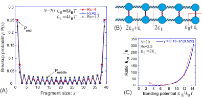
Figure 4: (A) The result of our calculation of statistical probability of thermal breakup of a two-stranded filament (parameters are labelled in the plot, note that we take the transverse binding to be the half of the longitudinal binding strength). The fragment size of 1 (or 39, for the two-stranded filament of length N=20) represents the single subunit dissociation; we can see a clear even-odd effect with the higher probability for the filament to break clean across the middle rather than have a complex-shape break. In (B) a sketch of this breakup mechanism is reported. The three data sets in the plot (A) show that there is no strong dependence on the cutoff distance $R_{c}$ of the potential. In (C) we plot the ratio of the end-dissociation rate $k_{\mathrm{off}}$ to the fragmentation rate $k_{-}$, as a function of strength of the physical bond $\varepsilon_{\|}$. At weak bonding, the reaction rate deviates from the Kramers thermal-activation law, but this is unlikely to be a relevant regime; at significant bonding strength the end/middle rate ratio clearly follows an exponential: $\exp[0.52\varepsilon/k_{\mathrm{B}}T]$ according to the fitting of our data.

II.4 Simulation results

The probability of a breakup event is directly proportional to the rate constant. We find that the ratio between the breakup rate at the filament end and the rate of fragmentation in the inner part of the filament is a strongly increasing function of $\varepsilon$, with an expected qualitative trend which is exponential (Arrhenius), $k_{\mathrm{off}}/k_{-}\approx\exp[0.52\varepsilon/k_{\mathrm{B}}T]$, as illustrated in fig. 4(C). This result can be rationalized using a simple argument based on the different connectivity at the end and in the middle. According to the Kramers escape rate theory 27-Kramers ; 28-Zaccone , the end-subunit escapes from the bonding minimum, with an exponential dependence on the total energy barrier, $k_{\mathrm{off}}\approx\exp[-(\varepsilon_{\|}+\varepsilon_{\bot})/k_{\mathrm{B}}T]=\exp[-1.5\varepsilon/k_{\mathrm{B}}T]$, since two bonds (one longitudinal and one transverse) need be broken, see fig. 4(B). Breakup in the middle, instead, involves the breaking of two longitudinal bonds; breakup of three bonds (two longitudinal, one transverse), or even more, is practically negligible because more cooperative and energetically unfavorable motion is required. Therefore we have $k_{-}\approx\exp[-2\varepsilon_{\|}/k_{\mathrm{B}}T]=\exp[-2\varepsilon/k_{\mathrm{B}}T]$. Upon forming the ratio, we readily obtain $k_{\mathrm{off}}/k_{-}=\exp[(\varepsilon_{\|}-\varepsilon_{\bot})/k_{\mathrm{B}}T]=\exp[0.5\varepsilon/k_{\mathrm{B}}T]$, in excellent agreement with the law found in simulations (the small deviation from 0.5 is certainly due to a proportion of rare complex-topology breaks). This result is very important because it establishes that, due to the different connectivity of subunits in the filament, the ratio between end-dissociation and fragmentation rates has to increase exponentially with the protein-protein binding energy $\varepsilon$.

II.5 Application to F-actin

For F-actin, Erickson9-Erickson has estimated the difference between the energy barriers for fragmentation and end-dissociation: $\sim$10.7 kcal/mol = 17.9$k_{\mathrm{B}}T$, giving the prediction $k_{\mathrm{off}}/k_{-}\approx 6\cdot 10^{7}$. This compares very well with the data assembled by Pollard and Cooper 19-Pollard , who quote the range for $k_{\mathrm{off}}\approx$ 0.5-5 $\mathrm{s}^{-1}$ and $k_{-}\approx 10^{-8}$ $\mathrm{s}^{-1}$. It should be noted that the fragment size distribution in the case of actin is, in reality, not symmetric at the two ends in the fast-polymerization or treadmilling limit, where the pointed end is made of ADP-actin subunits, whereas the barbed end is formed by ATP-actin, for which depolymerization is suppressed. The end-dissociation rates are $\sim$0.3 $\mathrm{s}^{-1}$ and $\sim$2 $\mathrm{s}^{-1}$ for the P-end and for the B-end, respectively, according to Pollard 8-Pollard ; 19-Pollard . However, the difference is less than an order of magnitude and does not introduce any substantial qualitative change in our picture. The rates are equal at both ends, and the distribution symmetric, in the opposite limit of slow polymerization at low monomer concentrations 2-Alberts .

Appendix A and Fig. 8 give more detail about F-actin filament and its bond structure. Applying the same analysis here with Pollard’s $2/3$ ratio for $\varepsilon_{\bot}/\varepsilon_{\|}$, we obtain $k_{\mathrm{off}}\approx\exp[-(\varepsilon_{\|}+\varepsilon_{\bot})/k_{\mathrm{B}}T]=\exp[-\frac{5}{3}\varepsilon/k_{\mathrm{B}}T]$, and $k_{-}\approx\exp[-(2\varepsilon_{\|}+\varepsilon_{\bot})/k_{\mathrm{B}}T]=\exp[-\frac{8}{3}\varepsilon/k_{\mathrm{B}}T]$. Hence, it follows that $k_{\mathrm{off}}/k_{-}=\exp[\varepsilon/k_{\mathrm{B}}T]$, that is, an Arrhenius dependence on the longitudinal binding energy. Comparing with the result for amyloids, fig. 4, the ratio between dissociation rate at the end and breakup rate in the middle is much larger for actin. This, for typical binding energy on the order of $20k_{\mathrm{B}}T$ (conservative estimate) gives an additional factor of $\sim e^{10}$ for actin $k_{\mathrm{off}}/k_{-}$ ratio, with respect to the case of amyloid. This means that dissociation rate at the end over breakup in the middle is $\sim e^{10}\approx 2.2\times 10^{4}$ times larger for actin than for amyloids. This estimate suggests that while breakup in the middle may play an important role in amyloids, it can be safely neglected in the dynamics of F-actin fibres.

In the remaining of this paper we focus on the amyloid system, for which the ‘ladder’ bond structure illustrated in fig. 4B) holds, and for which new experimental results are reported below.

II.6 Application to amyloid-like fibrils and comparison with experiments

For amyloid fibrils, using typical values of binding energy for $\beta$-sheets bonding in amyloid-like aggregates, which are on the order of 20-30$k_{\mathrm{B}}T$,29-Dobson our approach yields the prediction of $k_{\mathrm{off}}/k_{-}\approx 10^{5}$. In order to verify our prediction and the proposed molecular mechanism in amyloids, we experimentally determined the end-dissociation rate for insulin amyloid filaments exhibiting the typical two-stranded structure used in our model calculations, and compared it with the fragmentation rate estimated previously from kinetic fitting of total mass and length distribution: $k_{-}\approx 10^{-9}-10^{-8}$ $s^{-1}$ at T=60^∘C 16-Knowles ; 24-Smith . In this paper we obtain an estimate of $k_{\mathrm{off}}$ for insulin amyloid fibrils through direct observation of monomer release into solution as a function of time, as illustrated in fig. 5 and more details can be found in Appendix B. To this effect, a sample of mature insulin amyloid fibrils was first prepared at pH 2.0; we then isolated the fibrils by ultracentrifugation, and the supernatant, containing free monomer, was removed and replaced with a dilute aqueous solution of HCl, also at pH 2.0. In this manner we depleted an insulin amyloid fibril sample free of monomer. Over time, monomer dissociation from the fibril ends re-established the monomer-fibril equilibrium in the supernatant. To probe for soluble insulin during this process, we ultracentrifuged sample aliquots during a time course and investigated the supernatant solutions by gel electrophoresis as shown in fig. 5(B). These end-dissociation experiments were carried out at T=60^∘C, to match with existing literature data on $k_{-}$ , and also at T=4^∘C to allow better time-resolution of slower kinetics and to estimate the free energy barriers involved.

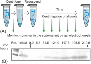
Figure 5: Experimental determination of monomer detachment rates from insulin amyloid fibrils. (A) A schematic showing how insulin fibrils were depleted of monomer and subsequently incubated. (B) The establishment of an equilibrium monomer population was monitored by SDS PAGE. Here a gel for a time course at 4^∘C is shown. From left to right, the gel contained: the reference band from a protein standard; the monomer from the initial fibril sample supernatant; the supernatants from the time points from 0 to 219.5 hours after the removal of the initial monomer population.

Assuming that fibril fragmentation is much slower compared to depolymerization, the concentration of free monomer as a function of time, $m(t)$, is given by the equilibrium monomer concentration, $m_{\mathrm{eq}}$, the number concentration of fibrils, $P$, and the dissociation rate constant $k_{\mathrm{off}}$, as: $m(t)=m_{\mathrm{eq}}[1-\exp(-2Pk_{\mathrm{off}}t/m_{\mathrm{eq}})]$. We determined a value for the product $Pk_{\mathrm{off}}$ through a least squares fit to the data in fig. 6. To find $m_{\mathrm{eq}}$ we calibrated the concentration at the plateau against a dilution series of known concentration, see Methods below. This analysis gave a value of $Pk_{\mathrm{off}}=1.3\cdot 10^{-10}$ M/s at 60^∘C and $1.2\cdot 10^{-12}$ M/s at 4^∘C. Considerations based on the average density, diameter and length of fibrils 24-Smith suggest that the average number of monomers per fibril is ca. 5000 (8.2 monomers per nm). Given the mass concentration of fibrils (2mM), this yields the concentration of fibrils $P=4\cdot 10^{-7}$ M, then $k_{\mathrm{off}}=3.3\cdot 10^{-4}$ $s^{-1}$ at 60^∘C. The same analysis gives $k_{\mathrm{off}}=3\cdot 10^{-6}$ 1/s at 4^∘C. Taking the value for the fragmentation rate of the same insulin fibrils, as measured previously 16-Knowles ; 24-Smith , the ratio becomes: $k_{\mathrm{off}}/k_{-}\approx 1.5\cdot 10^{5}$ at 60^∘C.

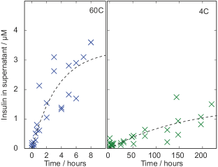
Figure 6: The measured concentration of soluble insulin against time, and the fit to the data, dashed line, at T=60^∘C and 4^∘C.

III Conclusions

Using the theoretically predicted (exponential) result in fig. 4(C) (and the value of T=60^∘C), we obtain the strength of the longitudinal physical bond between insulin subunits in the amyloid filament: $\varepsilon_{\|}\approx$ 13 kcal/mol = 22$k_{\mathrm{B}}T$. This is very close to our own ab-initio simulations of two-stranded F-actin in fig. 2(A), the results of molecular-dynamics work on amyloids 25-Han reproduced in fig. 2(B), and the common-sense expectation for a sequence of hydrogen bonds between two $\beta$-sheets. It also confirms our a priori assumption that the transverse bonding (mainly due to hydrophobic interactions) is approximately half in strength of $\varepsilon_{\|}$.

The availability of values for $k_{\mathrm{off}}$ at two different temperatures allows us to estimate the enthalpic barrier $\Delta H_{2}^{\ddagger}$ for the dissociation process, since $\ln[k_{\mathrm{off}}(1)/k_{\mathrm{off}}(2)]=\Delta H_{2}^{\ddagger}\cdot(1/k_{\mathrm{B}}T_{2}-1/k_{\mathrm{B}}T_{1})$. This yields $\Delta H_{2}^{\ddagger}\approx$ 16 kcal/mol, very close to the value of enthalpic barrier $\Delta H_{1}^{\ddagger}$ for the forward process measured previously 30-Buell .

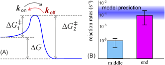
Figure 7: (A) A scheme of free energy levels and the barriers for aggregation and end-dissociation, $k_{\mathrm{on}}$ and _koff, respectively; the difference $\Delta G$ is essentially the bonding strength $\varepsilon$. It should be noted that in our simplified coarse-grained model we neglect rotational degrees of freedom (since our sub-units are perfect spheres), which means that some entropic contribution to the free energy is necessarily reapportioned to account for this - quantitatively precise estimates of free energy barriers can only be extracted from ab-initio simulations. (B) A pictorial comparison of the experimental data on breakup rates in insulin amyloid fibrils, from Ref.24 and this work.

In summary, we have shown that thermal breakup in a minimal model of typically two-stranded biomolecular filaments can be understood in a general way and depends exponentially on: 1) the topology of connectivity, 2) the difference in bonding energy in the longitudinal and transverse direction, and 3) the nature and asymmetry of the protein-protein interaction. All these effects strongly favour end-dissociation (detachment of a single protein from the filament ends) over the fragmentation of filament into two large fragments. In particular, for the most typical two-stranded structure observed in both actin and amyloid filaments, we establish the general law $k_{\mathrm{off}}/k_{-}=\exp[(\varepsilon_{\|}-\varepsilon_{\bot})/k_{\mathrm{B}}T]$ for amyloid fibrils, and a similar estimate for F-actin fibres gives $k_{\mathrm{off}}/k_{-}=\exp[\varepsilon/k_{\mathrm{B}}T]$. This important parameter is influenced by the nature of the protein-protein interaction (whether hydrophobicity- or hydrogen bond-controlled). With realistic values of binding energy from $\beta$-sheet bonding, this ratio reaches values on the order of $10^{4}$-$10^{5}$, an order-of-magnitude result which we were able to confirm experimentally on the example of insulin amyloid-like filaments, while the value for this ratio is comparatively much larger, in the order of $10^{8}$-$10^{9}$, for F-actin. These findings serve as the basis for improving the numerical description of protein aggregation phenomena within a common quantitative framework and, possibly, in future applications, for the development of pharmacologically-controlled cleavage of protein aggregates in vivo.

Appendices

III.1 MD simulation of subunit binding in F-actin

F-actin filament structure, as schematically depicted above in Fig. 8, was adopted from the extensive work of Voth et al. Chu-Voth ; Voth2011 , who have used a periodically repeating 13-monomer segment of F-actin with subunit structures taken from Protein Data Bank (PDB) structures 1J6Z (G-like; Otterbein ), 2ZWH  Oda , and 3MFP  Fujii and equilibrated it in waters with ADP as the bound nucleotide and Mg2+ at the high-affinity cationic bind site. Our starting point for the investigation of an effective binding potential was the PDB file of this 13-subunit long actin filament.

Our approach has been to fix all atom positions of the 12 subunits (A2-A13) and simulate moving of the center of mass of the terminal (A1) end-subunit along the line parallel to the filament axis. The energy change in this move is the potential reported in fig. 2(A). We first moved the whole A1 subunit with its atoms frozen with respect to its center of mass, and then equilibrated the ADP-bound actin molecule while keeping its center of mass fixed in its new position. The movement step of 0.5$\AA$ was found sufficient to give adequate resolution of the energy function, see fig. 2(A). The simulations were performed using the CHARM22 force field with CMAP correction and modified parameters for methylated histidine 31-Voth and the NAMD simulation code  NAMD . Both electrostatic and LJ potentials were truncated at a cutoff distance of 12$\AA$; in fact, we discovered that CHARM22 parameters are optimized for 12$\AA$ and larger cutoffs lead to distortions. Finally, the water (TIP3P model) was used to solvate the proteins.

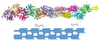
Figure 8: Two-stranded structure of 13-subunits long ADP-actin filament used in our simulations (the image is generated with PyMOL v. 1.7.7.2; the actin is shown in cartoon representation with each subunit is colored differently). The arrow shows the movement of the last subunit used to generate the energy function. The schematic of F-actin, indicating the bond-breaking energies, differs from the ‘ladder’ representation of amyloid filament in Fig. 4(B).

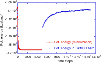
Figure 9: The illustration of NAMD simulation output for one point (the distance of 1.5$\AA$ from equilibrium for the end actin subunit being moved away from the filament). The first part of the plot shows the rapid and efficient energy minimization at T=0, followed by relatively slow equilibration in the heat bath at 300K.

For each simulation point (each position of the A1 center of mass) the procedure involved the energy minimization for 5000 steps, after which the system was heated to 300K and equilibrated for further 10000 steps. The illustration is given in fig. 9, for the point 1.5$\AA$ away from the equilibrium along the stretching axis; it appears convincing that a reasonable equilibration has taken place. After the whole sequence of simulations was completed (spanning the distance of A1 center of mass of -2$\AA$ to 20$\AA$, with zero defined as the equilibrium position) we have taken the value of system energy at the maximum separation as zero. Then the ‘binding energy’ reported in fig. 2(A) is the change with respect to that value: we recognize the deep attractive potential well and the steep repulsive rise of energy on compressing the distance – the characteristic features of the LJ potential used in the subsequent coarse-grained simulation.

III.2 Coarse-grained simulation of bond breakup

In our main computer simulation, we consider a coarse-grained model of protein filaments as 1D chains of Brownian particles where every particle is bonded to each of its two neighbors via the truncated Lennard- Jones potential, see fig. 10(A), where the distance $r$ between the two bonded particles is scaled by the parameter $\sigma$: is the hard-core diameter of the protein. We set the LJ potential to maintain a well depth equal to $\varepsilon$ , independently of the chosen cutoff radius $R_{c}$. When the two-stranded filament is considered, the transverse bonds have the potential depth $\varepsilon/2$ with the same cutoff.

We also include in our analysis the local bending energy. This effect is reflected in the finite energy one has to spend in order to bend the inter-protein bond, or equivalently, to change the angle between two adjacent bonds. Aiming to describe reasonably stiff filaments, we use the bending energy in the form $\frac{1}{2}K\theta^{2}$ , where $\theta_{i}$ is the angle between the directions of bonds from the particle $i$ to the preceding $(i-1)$ and the subsequent $(i+1)$ subunits. Figure 10(B) illustrates the way this effect is implemented by imposing pairs of equal and opposite forces on the joining bonds, providing a net torque on the junction. It is the same algorithm as used in, e.g. LAMMPS ‘angle-harmonic’ system LAMMPS . The bending modulus $K$, in units of $k_{B}T$, is directly related to the persistence length of the filament via the standard expression $l_{p}=K\sigma/k_{B}T$, where $\sigma$ is the ‘particle size’ in the LJ potential above.

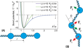
Figure 10: (A) An illustration of the role of truncation of the LJ potential at the cutoff distance $R_{c}$, while maintaining the fixed depth of the potential well $\varepsilon$. At larger $R_{c}$ the anharmonicity of the long-range attractive potential becomes more prominent (crucially, affecting the inflection point and the region of unstable concave potential shape). (B) The bond-bending penalty is implemented by forming two pairs of equal and opposite forces (couples) on the adjacent bonds to affect the bending angle $\theta$.

The dynamics is governed by the overdamped Langevin equation, which is discretized in the standard way; for each particle:

$$\bm{r}(t+\Delta t)=\bm{r}(t)-\frac{\Delta t}{\gamma}\nabla U(\{\bm{(}r)\})+\Gamma\sqrt{\frac{2\Delta t}{\gamma}}$$

where $\bm{r}$ is the 3n-dimensional vector containing the positions of all molecules, $\gamma$ is the friction coefficient for one particle moving in the medium, and $\Gamma$ is the amplitude of Gaussian stochastic force, defined according to the fluctuation-dissipation theorem. We used the $\Delta t=5\cdot 10^{-5}$ in MD units, and $\gamma=1$ since the friction incorporated into the value of $\Gamma$. The equation was integrated with an explicit Euler method.

Each run is initialized with interparticle distance $|r_{i}-r_{i-1}|=2^{1/6}\sigma$, corresponding to the minimum of the LJ interaction potentials, and terminated when any of the bonds reaches the cutoff $R_{c}$ . The location of the rupture was recorded. To generate the adequate statistics, $N$ independent runs were performed and the breakup probability calculated as $P_{i}=N_{i}/N$, where $N_{i}$ was the number of recorded breakup events for the bond $i\in(1...19)$. We used $N=10^{6}$ for the harmonic potential, $N=5\cdot 10^{4}$ for LJ potentials with $\varepsilon\leq 4k_{B}T$ and $N=3\cdot 10^{4}$ for LJ potentials with $\varepsilon>4k_{B}T$. Since runs were independent from each other, the $N_{i}$ are binomially (Bernoulli) distributed and the error bars were estimated as $3\sqrt{P_{i}(1-P_{i})/N}$. For the case of insulin, which has a diameter of about 2nm and $D\approx 2\cdot 10^{-10}\mathrm{m}^{2}/s$, the characteristic diffusion time is estimated as $\tau\approx$ 7ns. Our fixed numerical time step is then $\Delta t=(5\cdot 10^{-5})\tau\approx 0.5$ps.

The simulation application was written in C++ and took advantage of multi-core and multi-processor capabilities of the executing hardware. In the scenario where the LJ potential was acting in a repulsive manner on two particles, the simulation code was designed to handle the potentially unbounded resulting force. It would theoretically be possible within a fixed time step to find a pathological case where the force was too great and this would distort the results by creating an artificial ejection leading to a breakup where otherwise there would not have been one. To handle this an upper limit was selected on the force and if a calculated component was equal or greater than this limit the simulation would reset to the beginning of that time-step and re-execute it in 5 smaller time-steps. This feature was logged and it was determined that less than 0.25% of total execution time was spent in this specific case. Brownian motion components involved the use of pseudo-random number generation. The number generation was implemented using the Mersenne Twister algorithm Mersenne and a normal distribution parameterised by the mean and standard deviation was applied to the results. To ensure that no simulations were executed using a seed for the number generator that matched a prior execution run, seeds were taken to be fully 64-bit as opposed to the more customary 32-bit approach, and based on a unique temporal component selected as execution start time in compute cycles on the machine. This reduces the probability of matching/duplicate seeds to effectively zero. Finally the simulation itself performed multiple simulations concurrently. Each simulation was executed on a single thread with pre-emption for more effective resource scheduling, and the total number of simulations being executed in parallel was derived from the absolute total number of available hardware cores (accounting for extra thread capability from Hyper-Threading technology). This was done to allow more simulations to be run to satisfy the need for a statistically significant number of overall executions. In order to maximize performance simulation code was written in a lock-less fashion and the prevention of concurrency issues was accomplished through the use of Interlocked (or more colloquially ‘atomic’) operations on key synchronisation components.

III.3 Insulin amyloid dissociation measurements

Insulin fibrils were prepared using 0.5 mL 2 mM bovine insulin, 20 mM NaCl, HCl pH 2. The solution was filtered using a syringe driven filter (0.22 $\mu$m pore size, Millex), 1% v/v preformed fibrils were added to seed the reaction, the sample was then incubated at 65^∘C overnight. 200 $\mu$L of the mature fibril sample was then centrifuged in a Beckman ultracentrifuge at 90,000 rpm for 15 minutes at 4^∘C. These settings were used for all ultracentrifugation steps. The supernatant was kept as a reference for the monomer concentration. The pellet from 200 $\mu$L of the mature fibril solution was re-suspended in 2 mL 10 mM HCl and centrifuged in 200 $\mu$L aliquots. The supernatants from these were removed and replaced with 10 mM HCl, marking the beginning of the time course. The samples were incubated at either 4^∘C or 60^∘C to allow monomer dissociation. At each time point an aliquot was ultracentrifuged and the supernatant probed for soluble insulin as shown in fig. 5.

The time courses were repeated twice, two gels were run for each time course. For each temperature, the data from four gels has been combined in fig. 5(C). The SDS PAGE gels (NuPAGE 4-12% Bis-Tris, Life Technologies) were run in MES buffer at 200 V for 25 min using standard procedures, and protein bands were stained using the Silverquest kit (Life Technologies) according to the manufacturer instructions. On an SDS gel, insulin migrates as the two component peptides, the protein standard ladder seen in fig. 5(B) is therefore the 3 kDa band (insulin B chain) from the SeeBlue Plus 2 prestained standard (Life Technologies). The protein standard was also used as a band intensity reference between gels.

In order to evaluate $m_{\mathrm{eq}}$, gel electrophoresis was performed for the time points at the plateau of the time courses and a dilution series of insulin solutions. The results of a calibration gel for the time course at 4^∘C are shown in fig. 11. We obtained a calibration curve from a linear fit to the integral of the band intensity for the samples of known concentration. The equilibrium monomer concentration at 4^∘C was then found to be 1.5 $\mu$M and the one at 60^∘C to be 3.3 $\mu$M. The band intensities were measured with the gel image analysis tool in Ref. Schneider . The sum of the pixel intensities for each band was recorded as the band integral. For each gel, a line of best fit was determined for the signal intensity against the insulin concentration for the solutions of known concentration (purple points in fig. 11). This linear relationship was then used to determine $m_{\mathrm{eq}}$ from the band intensity at the plateau of a time course (green point in fig. 11).

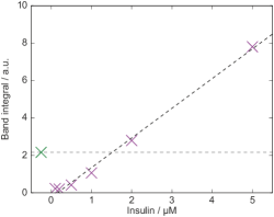
Figure 11: Calibration of the equilibrium monomer concentration. A linear fit to the integral of the band intensity for insulin solutions of known concentrations, purple. The time point at 219.5 hours from the experiments at 4^∘C was run on the same gel, green, we used the band integral of this fraction to determine $m_{\mathrm{eq}}$.

Acknowledgements

This research was supported by the ERC, EPSRC, BBSRC, and the Newman Foundation. Simulations were performed using the Darwin supercomputer of the University of Cambridge HPC Service (http://www.hpc.cam.ac.uk/), provided by Dell Inc. using Strategic Research Infrastructure funding from the Higher Education Funding Council for England. We are grateful to Dr. Marissa Saunders 31-Voth for providing a PDB file of the equilibrated actin filament structure used to generate Fig. 1.

References

- (1) F. Oosawa and S. Asakura, Thermodynamics of the Polymerization of Protein, (Academic Press, 1975, Waltham MA).
- (2) B. Alberts, Molecular Biology of the Cell, (Taylor & Francis, 2014, New York, 2002).
- (3) F. Chiti and C.M. Dobson, Protein misfolding, functional amyloid, and human disease, Annu. Rev. Biochem. 75, 333 (2006).
- (4) D. Chandler, Interfaces and the driving force of hydrophobic assembly, Nature 437, 640 (2005).
- (5) A. Irbáck, S.A. Jónsson, N. Linnemann, B. Linse, and S. Wallin, Aggregate geometry in amyloid fibril nucleation, Phys. Rev. Lett. 110, 058101 (2013).
- (6) A. Wegner, Spontaneous fragmentation of actin filaments in physiological conditions, Nature 296, 266 (1982).
- (7) A. Wegner and P. Savko, Fragmentation of actin filaments, Biochemistry 21, 1909-1913 (1982).
- (8) T.D. Pollard, Rate constants for the reactions of ATP-and ADP-actin with ends of actin filaments, J. Cell Biol. 193, 2747-2754 (1986).
- (9) H.P. Erickson, Co-operativity in protein-protein association, J. Molec. Biol. 296, 465-474 (1989).
- (10) H. J. Kinosian, L. A. Selden, J. E. Estes, L. C. Gershman, Actin filament annealing in the presence of ATP and phalloidin, Biochemistry 32, 12353-12357 (1993).
- (11) D. Sept, J. Xu, T.D. Pollard, and J.A. McCammon, Annealing accounts for the length of actin filaments formed by spontaneous polymerization, Biophys. J. 77, 2911-2919 (1999).
- (12) D. Vavylonis, Q. Yang, B. O’Shaughnessy, Actin polymerization kinetics, cap structure, and fluctuations, Proc. Natl. Acad. Sci. USA 102, 8543–8548 (2005).
- (13) E. B. Stukalin and A.B. Kolomeisky, ATP Hydrolysis Stimulates Large Length Fluctuations in Single Actin Filaments, Biophys. J. 90, 2673–2685 (2006).
- (14) E. Andrianantoandro, L. Blanchoin, D. Sept, J.A. McCammon, T.D. Pollard, Kinetic mechanism of end-to-end annealing of actin filaments, J. Molec. Biol. 312, 721-730 (2001).
- (15) I. Fujiwara1 and S. Takahashi and H. Tadakuma and T. Funatsu and S. Ishiwata, Microscopic analysis of polymerization dynamics with individual actin filaments, Nature Cell Biol. 4, 666-673 (2002).
- (16) J.R. Kuhn and T.D. Pollard, Real-time measurements of actin filament polymerization by total internal reflection fluorescence microscopy, Biophys. J. 88, 1387-1402 (2005).
- (17) J. Fass, C. Pak, J. Bamburg, A. Mogilner, Stochastic simulation of actin dynamics reveals the role of annealing and fragmentation, J. Theor. Biol. 252, 173-183 (2008).
- (18) T. P. J. Knowles and C. A. Waudby and G. L. Devlin and S. I. A. Cohen and A. Aguzzi and M. Vendruscolo and E. M. Terentjev and M. E. Welland and C. M. Dobson, An analytical solution to the kinetics of breakable filament assembly, Science 326, 1533-1537 (2009).
- (19) J. Adamcik and J.-M. Jung and J. Flakowski and P. De Los Rios, G. Dietler and R. Mezzenga, Understanding amyloid aggregation by statistical analysis of atomic force microscopy images, Nature Nanotech. 5, 423-428 (2010).
- (20) J. Käs, H. Strey, J.X. Tang, D. Finger, R. Ezzell, E. Sackmann, P.A. Janmey, F-actin, a model polymer for semiflexible chains in dilute, semi-dilute, and liquid crystalline solutions, Biophys. J. 70, 609-625 (1996).
- (21) T.D. Pollard, and J.A. Cooper, Actin and actin-binding proteins. A critical evaluation of mechanisms and functions, Annu. Rev. Biochem. 55, 987-1035 (1986).
- (22) N. Carulla et al., Molecular recycling within amyloid fibrils, Nature 436, 554-558 (2005).
- (23) M. Groenning, R.I. Campos, D. Hirschberg, P. Hammarstrom, B. Vestergaard, Considerably Unfolded Transthyretin Monomers Preceed and Exchange with Dynamically Structured Amyloid Protofibrils, Scie. Rep. 5, 11443 (2015).
- (24) C.F. Lee, Thermal breakage of a discrete one-dimensional string, Phys. Rev. E 80, 031134 (2009).
- (25) F. Gittes, B. Mickey, J. Nettleton, J. Howard, Flexural rigidity of microtubules and actin filaments measured from thermal fluctuations in shape, J. Cell Biol. 120, 923-934 (1993).
- (26) T.P.J. Knowles, J.F. Smith, A. Craig, C. M. Dobson, M.E. Welland, Spatial persistence of angular correlations in amyloid fibrils, Phys. Rev. Lett. 96, 238301 (2006).
- (27) T.P.J. Knowles, A.W. Fitzpatrick, S. Meehan, H.R. Mott, M. Vendruscolo, C.M. Dobson, and M.E. Welland, Role of intermolecular forces in defining material properties of protein nanofibrils, Science 318, 1900-1903 (2007).
- (28) E.B. Stukalin and A.B. Kolomeisky, Simple growth models of rigid multifilament biopolymers, J. Chem. Phys. 121, 1097 (2004).
- (29) J.F. Smith, T.P.J. Knowles, C.M. Dobson, C.E. Macphee, M.E. Welland, Characterization of the nanoscale properties of individual amyloid fibrils, Proc. Natl. Acad. Sci. USA 103, 15806–15811 (2006).
- (30) W. Han, K. Schulten, Fibril Elongation by A17−42: Kinetic network analysis of hybrid-resolution molecular dynamics simulations, J. Am. Chem. Soc. 136, 12450 (2014).
- (31) A. Zaccone, I. Terentjev, L. DiMichele, E.M. Terentjev, Fragmentation and depolymerisation of non-covalently bonded filaments, J. Chem. Phys. 142, 114905 (2015).
- (32) H.A. Kramers, Brownian motion in a field of force and the diffusion model of chemical reactions, Physica 7, 284 (1940).
- (33) A. Zaccone and E.M. Terentjev, Theory of thermally activated ionization and dissociation of bound states, Phys. Rev. Lett. 108, 038302 (2012).
- (34) J. L. Jiménez and E. J. Nettleton and M. Bouchard and C. V. Robinson and C. M. Dobson and H. R. Saibil, The protofilament structure of insulin amyloid fibrils, Proc. Natl. Acad. Sci. USA 99, 9196-9201 (2002).
- (35) A.K. Buell, J.R. Blundell, C.M. Dobson, M.E. Welland, E.M. Terentjev, T.P.J. Knowles, Frequency factors in a landscape model of filamentous protein aggregation, Phys. Rev. Lett. 104, 228101 (2010).
- (36) M.G. Saunders and G.A. Voth, Comparison between actin filament models: coarse-graining reveals essential differences, Structure 20, 641–653 (2012).
- (37) J.W. Chu, G.A. Voth, Allostery of actin filaments: Molecular dynamics simulations and coarse-grained analysis, Proc. Natl. Acad. Sci. USA 102, 13111-13116 (2005).
- (38) M.G. Saunders and G.A. Voth, Water molecules in the nucleotide binding cleft of actin: Effects on subunit conformation and implications for ATP hydrolysis, J. Mol. Biol. 413, 279 (2011).
- (39) L.R. Otterbein, P. Graceffa, R. Dominguez, The crystal structure of uncomplexated actin in the ADP state, Science 293, 708-711 (2001).
- (40) T. Oda, M. Iwasa, T. Aihara, Y. Maeda, A. Narita, The nature of the globular-to fibrous-actin transition, Nature 457, 441-445 (2009).
- (41) T. Fujii, A.H. Iwane, T. Yanagida, K. Namba, Direct visualization of secondary structures of F-actin by electron cryomicroscopy Nature 467, 724 (2010).
- (42) J.C. Phillips, et al., Scalable molecular dynamics with NAMD, J. Comp. Chem. 26, 1781-1802 (2005).
- (43) S. Plimpton, Fast parallel algorithms for short-range molecular dynamics, J. Comp. Phys. 117, 1-19 (1995).
- (44) M. Matsumoto and T. Nishimura, Mersenne twister: A 623-dimensionally equidistributed uniform pseudo-random number generator, ACM Trans. Mod. 8, 3-30 (1998).
- (45) C. A. Schneider, W.S. Rasband, and K. W. Eliceiri, NIH Image to ImageJ: 25 years of image analysis, Nat. Methods 9, 671-675 (2012).