A Formal Algebra for OLAP¹

Abstract

Online Analytical Processing (OLAP) comprises tools and algorithms that allow querying multidimensional databases. It is based on the multidimensional model, where data can be seen as a cube, where each cell contains one or more measures can be aggregated along dimensions. Despite the extensive corpus of work in the field, a standard language for OLAP is still needed, since there is no well-defined, accepted semantics, for many of the usual OLAP operations. In this paper, we address this problem, and present a set of operations for manipulating a data cube. We clearly define the semantics of these operations, and prove that they can be composed, yielding a language powerful enough to express complex OLAP queries. We express these operations as a sequence of atomic transformations over a fixed multidimensional matrix, whose cells contain a sequence of measures. Each atomic transformation produces a new measure. When a sequence of transformations defines an OLAP operation, a flag is produced indicating which cells must be considered as input for the next operation. In this way, an elegant algebra is defined. Our main contribution, with respect to other similar efforts in the field is that, for the first time, a formal proof of the correctness of the operations is given, thus providing a clear semantics for them. We believe the present work will serve as a basis to build more solid practical tools for data analysis.

Keywords: OLAP; Data Warehousing; Algebra; Data Cube; Dimension Hierarchy

.

1 Introduction

Online Analytical Processing(OLAP) [5] comprises a set of tools and algorithms that allow efficiently querying multidimensional (MD) databases containing large amounts of data, usually called Data Warehouses (DW). Conceptually, in the MD model, data can be seen as a cube, where each cell contains one or more measures of interest, that quantify facts. Measure values can be aggregated along dimensions, which give context to facts. At the logical level, OLAP data are typically organized as a set of dimension and fact tables. Current database technology allows alphanumerical warehouse data to be integrated for example, with geographical or social network data, for decision making. In the era of so-called “Big Data”, the kinds of data that could be handled by data management tools, are likely to increase in the near future. Moreover, OLAP and Business Intelligence (BI) tools allow to capture, integrate, manage, and query, different kinds of information. For example, alphanumerical data coming from a local DW, spatial data (e.g., temperature) represented as rasterized images, and/or economical data published on the semantic web. Ideally, a BI user would just like to deal with what she knows well, namely the data cube, using only the classical OLAP operators, like Roll-up, Drill-down, Slice, and Dice (among other ones), regardless the cube’s underlying data type. Data types should only be handled at the logical and physical levels, not at the conceptual level. Building on this idea, Ciferri et al. [2] proposed a conceptual, user-oriented model, independent of OLAP technologies. In this model, the user only manipulates a data cube. Associated with the model, there is a query language providing high-level operations over the cube. This language, called Cube Algebra, was sketched informally in the mentioned work. Extensive examples on the use of Cube Algebra presented in [7], suggest that this idea can lead to a language much more intuitive and simple than MDX, the de facto standard for OLAP. Nevertheless, these works do not give any evidence of the correctness of the languages and operations proposed, other than examples at various degrees of comprehensiveness. In fact, surprisingly, and in spite of the large corpus of work in the field, a formally-defined reference language for OLAP is still needed [6]. There is not even a well-defined, accepted semantics, for many of the usual OLAP operations. We believe that, far for being just a problem of classical OLAP, this formalization is also needed in current “Big Data” scenarios, where there is a need to efficiently perform real-time OLAP operations [3], that, of course, must be well defined.

Contributions

In this paper we (a) introduce a collection of operators that manipulate a data cube, and clearly define their semantics; and (b) prove, formally, that our operators can be composed, yielding a language powerful enough to express complex queries and cube navigation (“à la OLAP”) paths.

We achieve the above representing the data cube as a fixed $d$-dimensional matrix, and a set of $k$ measures, and expressing each OLAP operation as a sequence of atomic transformations. Each transformation produces a new measure, and, additionally, when a sequence forms an OLAP operation, a flag that indicates which are the cells that must be considered as input for the next operation. This formalism allows us to elegantly define an algebra as a collection of operations, and give a series of properties that show their correctness. We provide the proofs in the full paper. We limit ourselves to the most usual operations, namely slice, dice, roll-up and drill-down, which constitute the core of all practical OLAP tools. We denote these the classical OLAP operations. This allows us to focus on our main interest, which is, to prove the feasibility of the approach. Other not-so-usual operations are left for future work.

The main contribution of our work, with respect to other similar efforts in the field is that, for the first time, a formal proof to practical problems is given, so the present work will serve as a basis to build more solid tools for data analysis. Existing work either lacks of formalism, or of applicability, and no work of any of these kinds give sound mathematical prove of its claims. In this extended abstract we present the main properties, and leave the proofs for the full paper.

The remainder of the paper is organized as follows. In Section 2, we present our MD data model, on which we base the rest of our work. Section 3 presents the atomic transformations that we use to build the OLAP operations. In Section 4 we discuss the classical OLAP operations in terms of the transformations, show how they can be composed to address complex queries. We conclude in Section 5.

2 The OLAP Data Model

In this section we describe the OLAP data model we use in the sequel.

2.1 Multidimensional Matrix

We next give the definitions of multidimensional matrix schema and instance. In the sequel, $d$, with $d\geq 1$, is a natural number representing the number of dimensions of a data cube.

Definition 1 (Matrix Schema).

A $d$-dimensional matrix schema is a sequence $(D_{1},\allowbreak D_{2},\allowbreak...,\allowbreak D_{d})$ of $d$ dimension names.     $\sqcap$$\sqcup$

Dimension names can be considered to be strings. As illustrated in the following example, the convention will be that dimension names start with a capital letter.

Example 1.

The running example we use in this paper, deals with sales information of certain products, at certain locations, at certain moments in time. For this purpose, we will define a $3$-dimensional matrix schema $(D_{1},D_{2},D_{3})=(Product,\ Location,\ Time)$.     $\sqcap$$\sqcup$

Definition 2 (Matrix Instance).

A $d$-dimensional matrix instance (matrix, for short) over the $d$-dimensional matrix schema $(D_{1},D_{2},...,D_{d})$ is the product $dom(D_{1})\times dom(D_{2})\times\cdots\times dom(D_{d}),$ $i=1,2,...,d$, where $dom(D_{i})$ is a non-empty, finite, ordered set, called the domain, that is associated with the dimension name $D_{i}$. For all $i=1,2,...,d$, we denote by $<$, the order that we assume on the elements of $dom(D_{i})$. For $a_{1}\in dom(D_{1}),\allowbreak a_{2}\in dom(D_{2}),\allowbreak...,\allowbreak a_{d}\in dom(D_{d})$, we call the tuple $(a_{1},a_{2},...,a_{d})$, a cell of the matrix.     $\sqcap$$\sqcup$

The cells of a matrix serve as placeholders for the measures that are contained in the data cube (see Definition 7 below). Note that, as it is common practice in OLAP, we assumed an order $<$ on the domain. The role of the order is further discussed in Section 2.4.

As a notational convention, elements of the domains $dom(D_{i})$ start with a lower case letter, as it is shown in the following example.

Example 2.

For the $3$-dimensional matrix schema $(D_{1},D_{2},D_{3})\allowbreak=\allowbreak(Product,\ \allowbreak Location,\ \allowbreak Time)$ of Example 1, the non-empty sets $dom(D_{1})=\{lego,\allowbreak\ brio,\allowbreak\ apples,\allowbreak\ oranges\}$, $dom(D_{2})=\{antwerp,\ brussels,\ paris,\ marseille\}$, and $dom(D_{3})=\{\mbox{1/1/2014},\allowbreak\ ...,\allowbreak\ \mbox{31/1/2014}\}$ produce the matrix instance $dom(D_{1})\times\allowbreak dom(D_{2})\times\allowbreak dom(D_{3}).$ The cells of the matrix will contain the sales for each combination of values in the domain. In $dom(D_{2})$, we have, for instance, the order $antwerp<brussels<paris<marseille.$ Over the dimension $Time$, we have the usual temporal order.     $\sqcap$$\sqcup$

2.2 Level Instance, Hierarchy Instance and Dimension Graph

We now define the notions of dimension schema and instance.

Definition 3 (Dimension Schema, Hierarchy and Level).

Let $D$ be a name for a dimension. A dimension schema $\sigma(D)$ for $D$ is a lattice, with a unique top-node, called $All$ (which has only incoming edges) and a unique bottom-node, called $Bottom$ (which has only outgoing edges), such that all maximal-length paths in the graph go from $Bottom$ to $All$. Any path from $Bottom$ to $All$ in a dimension schema $\sigma(D)$ is called a hierarchy of $\sigma(D)$. Each node in a hierarchy (i.e., in a dimension schema) is called a level (of $\sigma(D)$).     $\sqcap$$\sqcup$

As a convention, level names start with a capital letter. Note that the $Bottom$ node is often renamed, depending on the application.

Example 3.

Fig. 1 gives examples of dimension schemas $\sigma(Location)$ and $\sigma(Time)$ for the dimensions $Location$ and $Time$ in Example 1. For the dimension $Location$, we have $Bottom=City$, and there is only one hierarchy, denoted $City\rightarrow Region\rightarrow Country\rightarrow All.$ The node $Region$ is an example of a level in this hierarchy. For the dimension $Time$, we have $Bottom=Day$, and two hierarchies, namely $Day\rightarrow Month\rightarrow Semester\rightarrow Year\rightarrow All$ and $Day\rightarrow Week\rightarrow All$.     $\sqcap$$\sqcup$

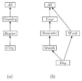
Figure 1: Dimension schemas for the dimensions $Location$, in ($a$), and $Time$ , in ($b$).

Definition 4 (Level Instance, Hierarchy Instance, Dimension Graph).

Let $D$ be a dimension with schema $\sigma(D)$, and let $\ell$ be a level of $\sigma(D)$. A level instance of $\ell$ is a non-empty, finite set $dom(D.\ell)$. If $\ell=All$, then $dom(D.All)$ is the singleton $\{all\}$. If $\ell=Bottom$, then $dom(D.Bottom)$ is the the domain of the dimension $D$, that is, $dom(D)$ (as in Definition 2).

A dimension graph (or instance) $I(\sigma(D))$ over the dimension schema $\sigma(D)$ is a directed acyclic graph with node set $\bigcup_{\ell}dom(D.\ell),$ where the union is taken over all levels in $\sigma(D)$. The edge set of this directed acyclic graph is defined as follows. Let $\ell$ and $\ell^{\prime}$ be two levels of $\sigma(D)$, and let $a\in dom(D.\ell)$ and $a^{\prime}\in dom(D.\ell^{\prime})$. Then, only if there is a directed edge from $\ell$ to $\ell^{\prime}$ in $\sigma(D)$, there can be a directed edge in $I(\sigma(D))$ from $a$ to $a^{\prime}$.

If $H$ is a hierarchy in $\sigma(D)$, then the hierarchy instance (relative to the dimension instance $I(\sigma(D))$) is the subgraph of $I(\sigma(D))$ with nodes from $dom(D.\ell)$, for $\ell$ appearing in $H$. This subgraph is denoted $I_{H}(\sigma(D))$.     $\sqcap$$\sqcup$

As notational convention, the names of objects in a set $dom(D.\ell)$ start with a lower case character. We remark that a hierarchy instance $I_{H}(\sigma(D))$ is always a (directed) tree. Also, if $a$ and $b$ are two nodes in a hierarchy instance $I_{H}(\sigma(D))$, such that $(a,b)$ is in the transitive closure of the edge relation of $I_{H}(\sigma(D))$, we will say that $a$ rolls-up to $b$ and we denote this by $\rho_{H}(a,b)$ (or $\rho(a,b)$ if $H$ is clear from the context).

Example 4.

Consider the $Location$ dimension, whose schema $\sigma(Location)$ is given in Fig. 1 ($a$). From Example 2, we have $dom(Location)=\{antwerp,$ $\ brussels,$ $\ paris,$ $\ marseille\}$, which is $dom(Location.Bottom)$, or $dom(Location.City)$.

An example of a dimension instance $I(\sigma(Location))$ is depicted in Fig. 2. This example expresses, for instance, that the city $brussels$ is located in the region $capital$ which is part of the country $belgium$, meaning that $brussels$ rolls-up to $capital$ and to $belgium$, that is, $\rho(brussels,\ captial)$ and $\rho(brussels,\ belgium)$.     $\sqcap$$\sqcup$

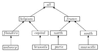
Figure 2: An example of a dimension graph (or instance) $I(\sigma(Location))$.

In a dimension graph, we must guarantee that rolling-up through different paths gives the same results. This is formalized by the concept of “sound” dimension graph.

Definition 5 (Sound Dimension Graph).

Let $I(\sigma(D))$ be a dimension graph (as in Definition 4). We call this dimension graph sound, if for any level $\ell$ in $\sigma(D)$ and any two hierarchies $H_{1}$ and $H_{2}$ that reach $\ell$ from the $Bottom$ level and any $a\in dom(D)$ and $b_{1},b_{2}\in dom(D.\ell)$, we have that $\rho_{H_{1}}(a,b_{1})$ and $\rho_{H_{2}}(a,b_{2})$ imply that $b_{1}=b_{2}$.     $\sqcap$$\sqcup$

In this paper, we assume that dimension graphs are always sound.

2.3 Multidimensional Data Cube

Essentially, a data cube is a matrix in which the cells are filled with measures that are taken from some value domain $\Gamma$. For many applications, $\Gamma$ will be the set of real or rational numbers, although some other ones may include, e.g., spatial regions or geometric objects.

Definition 6 (Data Cube Schema).

A $d$-dimensional data cube schema consists of (a) a $d$-dimensional matrix schema $(D_{1},D_{2},...,D_{d})$; and (b) a hierarchy schema $\sigma(D_{i})$ for each dimension $D_{i}$, with $i=1,2,...,d$.     $\sqcap$$\sqcup$

Definition 7 (Data Cube Instance).

Let $\Gamma$ be a non-empty set of “values”. A $d$-dimensional, $k$-ary data cube instance (or data cube, for short) $\cal D$ over the $d$-dimensional matrix schema $(D_{1},D_{2},...,D_{d})$ and hierarchy schemas $\sigma(D_{i})$ for $D_{i}$, for $i=1,2,...,d$, with values from $\Gamma$, consists of (a) a $d$-dimensional matrix instance over the matrix schema $(D_{1},D_{2},...,D_{d})$, $M({\cal D})$; (b) for each $i=1,2,...,d$, a sound dimension graph $I(\sigma(D_{i}))$ over $\sigma(D_{i})$; (c) $k$ measures $\mu_{1},\mu_{2},...,\mu_{k}$, which are functions from $dom(D_{1})\times dom(D_{2})\times\cdots\times dom(D_{d})$ to the value domain $\Gamma$; and (d) a flag $\varphi$ , which is a function from $dom(D_{1})\times\cdots\times dom(D_{d})$ to the set $\{0,1\}$.     $\sqcap$$\sqcup$

In the remainder of this paper we assume that $\Gamma={\bf Q}$, the set of the rational numbers. For most applications, this suffices. Also, as a notational convention, we use calligraphic characters, like $\cal D$, to represent data cube instances.

The flag $\varphi$ can be considered as a $(k+1)$-st Boolean measure. The role of $\varphi$ is to indicate which of the matrix cells are currently “active”. The active cells have a flag value $1$ and the others have a flag value $0$. When we operate over a data cube, flags are used to indicate the input or output parts of the matrix of the cube. Typically, in the beginning of the operations, all cells have a flag value of $1$. The role of flags will become more clear in the next sections, when we discuss OLAP transformations and operations.

2.4 Ordered Domains and the Representation of Higher-level Objects

When performing OLAP transformations and operations, we may need to store aggregate information about certain measures up to some level above the $Bottom$ one. We do not want to use extra space for this in the data cube. Instead, we use the available cells of the original data cube to store this information. For this, we make use of the order assumed in Definition 2, for the representation of high-level objects by $Bottom$-level objects.

Definition 8.

Let $D\in\{D_{1},D_{2},...,D_{d}\}$ be an arbitrary dimension with domain $dom(D)=dom(D.Bottom)$. Let $\ell$ be a level of $\sigma(D)$. An element $b\in dom(D.\ell)$ is represented by the smallest element $a\in dom(D)$ (according to $<$) for which $\rho(a,b)$ holds. We denote this as $rep(b)=a$, and say that $a$ represents $b$.     $\sqcap$$\sqcup$

Example 5.

Continuing with the previous examples, we consider the dimension $Location$ with $dom(Location)=\{antwerp,\ \allowbreak brussels,\ \allowbreak paris,\ \allowbreak marseille\}$ (i.e., $dom(Location.City)$. On this set, we assume the order $antwerp<brussels<paris<marseille$. For this dimension, we have the hierarchy and the dimension instance, given in Figs. 1 and  2, respectively. At the $Bottom=City$ level, cities represent themselves. At higher levels, regions and countries are represented by their “first” city in $dom(Location)$ (according to $<$). Thus, $flanders$ and $belgium$ are represented by $antwerp$, $france$ is represented by $paris$, and $south$ is represented by $marseille$. At the level $All$, $antwerp$ represents $all.$     $\sqcap$$\sqcup$

Note that the $Bottom$-level representatives of higher-level objects, will be flagged $1$, and other cells flagged $0$. Also, in our example, if we aggregate information at level $Region$, with $dom(Location.Region)=\allowbreak\{flanders,\ \allowbreak capital,\ \allowbreak north,\ \allowbreak south\}$, then all cities in $dom(Location)$ become flagged. Thus, it would not be clear if the cube contains information at the level $City$ or at the level $Region$. To solve this, we could keep a log of the OLAP operations that are performed, making the level of aggregation clear. The following property shows how the order on the $Bottom$ level induces and order on higher levels.

Property 1.

Let $D\in\{D_{1},D_{2},...,D_{d}\}$ be a (sound) dimension of a data cube $\cal D$ and let $\ell$ be a level in the dimension schema $\sigma(D)$. The order $<$ on $dom(D)$ induces an order on $dom(D.\ell)$ as follows. If $b_{1},b_{2}\in dom(D.\ell)$, then $b_{1}<b_{2}$ if and only if $rep(b_{1})<rep(b_{2})$.     $\sqcap$$\sqcup$

3 OLAP Transformations and Operations

A typical OLAP user manipulates a data cube by means of well-known operations. For instance, using our running example, the query “Total sales by region, for regions in Belgium or France”, is actually expressed as a sequence of operations, whose semantics should be clearly defined, and which can be applied in different order. For example, we can first apply a Roll-Up (i.e., an aggregation) to the Country level, and once at that level apply a Dice operation, which keeps the cube cells corresponding to Belgium or France. Finally, a Drill-Down can be applied to disaggregate the sales down to the level Region, returning the desired result. In what follows, we characterize OLAP operations as the result of sequences of “atomic” OLAP transformations, which are measure-creating updates to a data cube.

3.1 Introduction to OLAP Transformations and Operations

An atomic OLAP transformation acts on a data cube instance, by adding a measure to the existing data cube measures. OLAP operations like the ones informally introduced above are defined, in our approach, as a sequence of transformations. The process of OLAP transformations starts from a given input data cube ${\cal D}_{in}$. We assume that this original data cube has $k$ given measures $\mu_{1},\mu_{2},...,\mu_{k}$ (as in Definition 7). These $k$ measures have a special status in the sense that they are “protected” and can never be altered (see Section 3.2). However, there is one exception to this protection. These original measures can be “destroyed” in some cells (see further on), for instance, as the result of slice or dice operations, which are destructive by nature. Operations of these types destroy the content of some matrix cells and remove even the protected measures in it.

Typically, the input-flag $\varphi$ of the original data cube ${\cal D}_{in}$ is set to $1$ in every cell and signals that every cell of $M({\cal D}_{in})$ is part of the input cube.

Atomic OLAP transformations can be applied to data cubes. They add (or create) new measures to the sequence of existing measures by adding new measure values in each cell of the data cube’s matrix. At any moment in this process, we may assume that the data cube $\cal D$ has $k+l$ measures $\mu_{1},\mu_{2},...,\mu_{k};\tau_{1},...,\tau_{l}$, where the first $k$ are the original measures of ${\cal D}_{in}$, and the last $l$ (with $l\geq 0$) ones have been created subsequently by $l$ OLAP transformations (where $\tau_{1},...,\tau_{l}$ is the empty sequence of $\tau$’s, for $l=0$). The next OLAP transformation adds a new measure $\tau_{l+1}$ to the matrix cells.

We have said that we use OLAP transformations to compute OLAP operations. We indicate that the computation of an OLAP operation $O$ is finished by creating an $m$-ary output flag $\varphi^{(m)}_{O}$. This output flag is a Boolean measure, that is created via atomic OLAP transformations. It indicates which of the cells of $M({\cal D})$ should be considered as belonging to the output of $O$. It is $m$-ary in the sense that it keeps the last $m$ created measures $\tau_{l-m+1},\tau_{l-m+2},...,\tau_{l}$ and “trashes” the rest. It also removes the previous flag, which it replaces. The initial measures $\mu_{1},\mu_{2},...,\mu_{k}$ of the input data cube ${\cal D}_{in}$ are never removed (unless they are “destroyed” in some cells). They remain in the cube throughout the process of applying one OLAP operation after another to ${\cal D}_{in}$, and can be used at any stage. Summarizing, after an OLAP operation of output arity $m$ is completed on some cube $\cal D$, the measures in the cells of the output data cube ${\cal D}^{\prime}=O({\cal D})$ are of the form $\underline{\mu_{1},\mu_{2},...,\mu_{k}};\tau_{l-m+1},\tau_{l-m+2},...,\tau_{l};\varphi^{(m)}_{O}.$ Here, the underlining indicates the protected status of these measures. After each OLAP operation, we do a “cleaning” by renaming the unprotected measures with the symbols $\tau_{1},\tau_{2},...,\tau_{m}$ and the output measures become $\underline{\mu_{1},\mu_{2},...,\mu_{k}};\tau_{1},\tau_{2},...,\tau_{m};\varphi^{(m)}_{O}.$ The next OLAP operation $O^{\prime}$ can then act on ${\cal D}^{\prime}$ and use in its computation all the measures above. We remark that the dimensions, the hierarchy schemas and instances of $\cal D$ remain unaltered during the entire OLAP process.

We end this description with a remark on destructors. A destructor, optionally, precedes the creation of an output flag. A destructor $\delta$ takes the value $1$ for some cells of the matrix of a data cube, and $0$ on other cells. When $\delta$ is invoked (and activated by the output flag that follows it) on a data cube $\cal D$ with measures $\underline{\mu_{1},\mu_{2},...,\mu_{k}};\tau_{1},\tau_{2},...,\tau_{m}$ and flag $\varphi^{(m)}_{O}$, it empties all cells for which the value of the destructor $\delta$ is $0$ by removing all measures from them, even the protected ones, thereby effectively “destroying” these cells. This is the only case where the protected measures are altered (see operations Slice or Dice, later). The output of a destructive operation $O$ looks like $\underline{\mu_{1},\mu_{2},...,\mu_{k}};\tau_{1},\tau_{2},...,\tau_{l};\delta;\varphi^{(m)}_{O},$ in which the destructor precedes the output flag. The effect of the presence of a destructor is the following. A cell such that $\delta=0$ is emptied, after which it contains no more measures and flag. For cells with $\delta=1$, the sequence of measures $\underline{\mu_{1},\mu_{2},...,\mu_{k}};\allowbreak\tau_{1},\tau_{2},...,\tau_{l};\allowbreak\delta;\varphi^{(m)}_{O};$ is transformed to $\underline{\mu_{1},\mu_{2},...,\mu_{k}};\allowbreak\tau_{l-m+1},\allowbreak\tau_{l-m+2},\allowbreak...,\allowbreak\tau_{l};\allowbreak\varphi^{(m)}_{O};$ which is renamed as $\underline{\mu_{1},\mu_{2},...,\mu_{k}};\tau_{1},\tau_{2},...,\tau_{m};\varphi;$ before the next transformation takes place. This transformation will act, cell per cell, on the matrix of a cube, and it does nothing with emptied cells. That is, no new measure can ever be added to a destroyed cell.

The following definition specifies how an OLAP transformation acts on a data cube. We then address in detail each atomic OLAP transformation appearing in this definition.

Definition 9 (OLAP Transformation).

Let $\cal D$ be a $d$-dimensional, $(k+l)$-ary data cube instance with given (or protected) measures $\mu_{1},\mu_{2},...,\mu_{k}$, created measures $\tau_{1},...,\tau_{l}$ (with $l\geq 0$) and flag $\varphi$ over some value domain $\Gamma$. An OLAP transformation $T$, applied to $\cal D$, results in the creation of a new measure $\tau_{l+1}$ in $\cal D$. Transformation $T$ adds measure $\tau_{l+1}$ to non-empty cells of $M({\cal D})$; $\tau_{l+1}$ is produced from: $\mu_{1},\mu_{2},...,\mu_{k}$ (in non-empty cells); $\varphi$ (in non-empty cells); $\tau_{1},\tau_{2},...,\tau_{l}$ (in non-empty cells) and the hierarchy schemas and instances of $\cal D$; and belongs to one of the following classes: (a) Arithmetic transformations (Definition 11); (b) Boolean transformations (Definition 12); (c) Selectors (Definition 13); (d) Counting, sum, min-max (Definitions 14, 19); (e) Grouping (Definition 18).

An OLAP transformation can also result in the creation of a measure that is an output flag $\varphi^{(m)}$ of arity $m$. This should be a measure with a Boolean value. To indicate that it is a flag of arity $m$, we use the reserved symbol $\varphi^{(m)}$ instead of $\tau_{l+1}$. An output flag $\varphi^{(m)}$ may (optionally) be preceded by a destructor $\delta$. This should be a measure with a Boolean value (to indicate which cells are destroyed). We use the reserved symbol $\delta$ instead of $\tau_{l+1}$.     $\sqcap$$\sqcup$

3.2 OLAP Operations and their Composition

Before we give the definition of an OLAP operation, we describe the input to the OLAP process (this process may involve multiple OLAP operations). Such input is a $d$-dimensional, $k$-ary data cube instance ${\cal D}_{in}$, with measures $\mu_{1},\mu_{2},...,\mu_{k}$ and flag $\varphi$. These measures are protected in the sense that they remain the first $k$ measures throughout the entire OLAP process and are never altered or removed unless they are destroyed in some cells. The cube ${\cal D}_{in}$ has also a Boolean flag $\varphi$, which typically has value $1$ in all cells of $M({\cal D}_{in})$. Thus, the measures of the input cube ${\cal D}_{in}$ are denoted $\underline{\mu_{1},\mu_{2},...,\mu_{k}};\varphi.$

After applying a sequence of OLAP operations to ${\cal D}_{in}$, we obtain a data cube ${\cal D}$.

Definition 10 (OLAP Operation).

Let $\cal D$ be a $d$-dimensional, $(k+l)$-ary input data cube instance with given measures $\mu_{1},\mu_{2},...,\mu_{k}$, computed measures $\tau_{1},...,\tau_{l}$ and flag $\varphi$. The data cube $\cal D$ acts as the input of an OLAP operation $O$ (of arity $m$), which consists of a sequence of $n$ consecutive OLAP transformations that create the additional measures $\tau_{l+1},...,\tau_{l+n}$, followed by the creation of an $m$-ary flag $\varphi^{(m)}_{O}$ (possibly preceded by a destructor $\delta$). As the result of the creation of $\varphi^{(m)}_{O}$, the measures in the cells of the data cube are changed from $\underline{\mu_{1},\mu_{2},...,\mu_{k}};\tau_{1},...,\tau_{l};\varphi;\tau_{l+1},...,\tau_{l+n}$ to $\underline{\mu_{1},\mu_{2},...,\mu_{k}};\tau_{l+n-m+1},...,\tau_{l+n};\varphi^{(m)}_{O},$ which become $\underline{\mu_{1},\mu_{2},...,\mu_{k}};\tau_{1},...,\tau_{m};\varphi,$ after renaming. The output cube ${\cal D}^{\prime}=O({\cal D})$ has the same dimensions, hierarchy schemas and instances as ${\cal D}$, and measures $\underline{\mu_{1},\mu_{2},...,\mu_{k}};$ $\tau_{1},...,\tau_{m};\varphi.$ In the case where $\varphi^{(m)}_{O}$ is preceded by a destructor $\delta$, the same procedure is followed, except for the cells of $M({\cal D})$ for which $\delta$ takes the value $0$. These cells of $M({\cal D})$ are emptied, contain no measures, and become inaccessible for future transformations.     $\sqcap$$\sqcup$

3.3 Atomic OLAP Transformations

We now address the five classes of atomic OLAP transformations of Definition 9. We use the following notational convention. For a measure $\alpha$, we write $\alpha(x_{1},\allowbreak x_{2},...,\allowbreak x_{d})$ to indicate the value of $\alpha$ in the cell $(x_{1},\allowbreak x_{2},...,\allowbreak x_{d})\in dom(D_{1})\times dom(D_{2})\times\cdots\times dom(D_{d}).$ We remark that $\alpha(x_{1},\allowbreak x_{2},...,\allowbreak x_{d})$ does not exist for empty cells and it is thus not considered in computations. Also, we assume that there are protected measures $\mu_{1},\mu_{2},...,\mu_{k}$, and computed measures $\tau_{1},...,\tau_{l}$ in the non-empty cells, and call $\tau_{l+1}$ the next computed measure.

3.3.1 Arithmetic Transformations

Definition 11 (Arithmetic Transformations).

The following creations of a new measure $\tau_{l+1}$ are arithmetic transformations:

1. (Rational constant) $\tau_{l+1}=\alpha$, with $\alpha\in{\bf Q}$, a rational number.

2. (Sum) $\tau_{l+1}=\alpha+\beta$, with $\alpha,\beta\in\{\mu_{1},\mu_{2},...,\mu_{k},\tau_{1},\allowbreak\tau_{2},\allowbreak...,\allowbreak\tau_{l}\}$.

3. (Product) $\tau_{l+1}=\alpha\cdot\beta$, with $\alpha,\beta\in\{\mu_{1},\mu_{2},...,\mu_{k},\tau_{1},\allowbreak\tau_{2},\allowbreak...,\allowbreak\tau_{l}\}$.

4. (Quotient) $\tau_{l+1}=\alpha/\beta$, with $\alpha,\beta\in\{\mu_{1},\mu_{2},...,\mu_{k},\tau_{1},\allowbreak\tau_{2},\allowbreak...,\allowbreak\tau_{l}\}$. Here, by convention, $a/0:=a$ for all $a\in{\bf Q}$.     $\sqcap$$\sqcup$

3.3.2 Boolean Transformations

Definition 12 (Boolean Transformations).

The following creations of a new measure $\tau_{l+1}$ are Boolean transformations:

1. (Equality test on measures) $\tau_{l+1}=(\alpha=\beta)$, with $\alpha,\beta\in\{\mu_{1},\allowbreak\mu_{2},\allowbreak...,\allowbreak\mu_{k},\allowbreak\tau_{1},\allowbreak\tau_{2},\allowbreak...,\allowbreak\tau_{l}\}$. Here, the result of $(\alpha=\beta)$ is a Boolean 1 or 0 (cell per cell in the non-empty cells of the matrix).

2. (Comparison test on measures) $\tau_{l+1}=(\alpha<\beta)$, with $\alpha,\beta\in\{\mu_{1},\allowbreak\mu_{2},\allowbreak...,\allowbreak\mu_{k},\allowbreak\tau_{1},\allowbreak\tau_{2},\allowbreak...,\allowbreak\tau_{l}\}$. Here, the result of the comparison $(\alpha<\beta)$ is a Boolean 1 or 0 (cell per cell in the non-empty cells of the matrix).

3. (Equality test on levels) For a level $\ell$ in the dimension schema $\sigma(D_{i})$ of dimension $D_{i}$, and a constant object $c\in dom(D_{i}.\ell)$, $\tau_{l+1}(x_{1},\allowbreak x_{2},...,\allowbreak x_{d})=(\ell=c)$ is an “equality” test. Here, the result of $(\ell=c)$ is a Boolean 1 or 0 (cell per cell in the non-empty cells of the matrix) such that $\tau_{l+1}(x_{1},\allowbreak x_{2},...,\allowbreak x_{d})$ is $1$ if and only if $x_{i}$ rolls-up to $c$ at level $\ell$, that is $\rho(x_{i},c)$.

4. (Comparison test on levels) For a level $\ell$ in the dimension schema $\sigma(D_{i})$ of dimension $D_{i}$, and a constant $c\in dom(D_{i}.\ell)$, $\tau_{l+1}(x_{1},\allowbreak x_{2},...,\allowbreak x_{d})=(\ell<_{\ell}c)$ is a “comparison” test. The result of $(\ell<_{\ell}c)$ is a Boolean 1 or 0 (cell per cell in the non-empty cells of the matrix), such that $\tau_{l+1}(x_{1},\allowbreak x_{2},...,\allowbreak x_{d})$ is $1$ if and only if $x_{i}$ rolls-up to an object $b$ at level $\ell$ for which $b<_{\ell}c$. The order $<_{\ell}$ can be any order that is defined on level $\ell$. Transformation $\tau_{l+1}(x_{1},\allowbreak x_{2},...,\allowbreak x_{d})=(c<_{\ell}\ell)$ is defined similarly.     $\sqcap$$\sqcup$

Example 6.

We illustrate the use of Boolean transformations by means of a sequence of transformations that implement a “dice” (see Section 4.2 for more details). The query $\mbox{\sf DICE}({\cal D},sales>50)$ asks for the cells in the matrix of $\cal D$ which contain sales that are higher than 50. This query can be implemented by the following sequence of transformations:

• $\tau_{1}=49.99$ (rational constant);

• $\tau_{2}=(\tau_{1}<sales)$ (comparison test on measures);

• $\tau_{3}=\mu_{1}\cdot\tau_{2}$ (product);

• $\delta=\tau_{2}$ (destructor); and

• $\varphi^{(1)}=\tau_{2}$ (unary flag)

The measure $\tau_{3}$ contains the $sales$ values larger than or equal to 50 (and a 0 if the $sales$ are lower). The destructor $\delta$ destroys the cells that contain a O. Finally, the flag $\varphi^{(1)}$ selects all cells from the input as output cells (it will contain a 1 for all such cells that satisfy the condition), and concludes the $\mbox{\sf DICE}({\cal D},sales>50)$ operation. The output of this operation is $\underline{sales};\tau_{3};\varphi^{(1)},$ which is then renamed to $\underline{sales};\tau_{1};\varphi.$     $\sqcap$$\sqcup$

3.3.3 Selectors

Definition 13 (Selector Transformations).

The following creations of a new measure $\tau_{l+1}$ are selector transformations (or selectors), and their definition is cell per cell of $M({\cal D})$:

1. (Constant selector) For a level $\ell$ in the dimension schema $\sigma(D_{i})$ of a dimension $D_{i}$, and $c\in dom(D_{i}.\ell)$, $\tau_{l+1}$ can be a constant-selector for $c$, denoted $\sigma_{D_{i}.\ell=c}$, and it corresponds to the equality test on levels $\tau_{l+1}(x_{1},\allowbreak x_{2},...,\allowbreak x_{d})=(\ell=c)$.

2. (Level selector) For a level $\ell$ in the dimension schema $\sigma(D_{i})$ of a dimension $D_{i}$, $\tau_{l+1}$ can be a level-selector for $\ell$, denoted by $\sigma_{D_{i}.\ell}$, which means that we have, for all $x_{j}\in dom(D_{j})$ with $j\not=i$,

   $$\tau_{l+1}(x_{1},...,x_{i_{1}},a,x_{i+1},...,x_{d})=\left\{\begin{array}[]{l l}1&\mbox{if}~{}a=rep(b){}\\ &\mbox{for some}~{}b\in dom(D_{i}.\ell),\\ 0&\mbox{otherwise. }\\ \end{array}\right.$$

   $\sqcap$$\sqcup$

The constant selector in Definition 13, corresponds to the equality test on levels (see 3. in Definition 12). Here, this transformation appears with a different functionality and we reserve a special notation for it, and we repeated it. Also, note that the level selector selects all representatives (at the $Bottom$ level) of objects at level $\ell$ of dimension $D_{i}$.

Example 7.

The query $\mbox{\sf DICE}({\cal D},Location.City=antwerp\ OR\ Location.City=brussels),$ asks for the sales in the cities of $antwerp$ and $brussels$. It can be implemented by the following sequence of transformations, where $\tau_{3}$ can take values $0$ or $1$, since the cities $antwerp$ and $brussels$ do not overlap:

• $\tau_{1}=\sigma_{Location.City=antwerp}$ (constant selector);

• $\tau_{2}=\sigma_{Location.City=brussels}$ (constant selector);

• $\tau_{3}=\tau_{1}+\tau_{2}$ (sum);

• $\tau_{4}=\tau_{3}\cdot\mu_{1}$ (product);

• $\delta=\tau_{3}$ (destroys the cells outside $antwerp$ and $brussels$);

• $\varphi^{(1)}=\tau_{3}$ (unary flag creation).

$\sqcap$$\sqcup$

3.3.4 Count, Sum and Min-Max

Definition 14 (Counting, Sum, and Min-Max Transformations).

The creations of a new measure $\tau_{l+1}$ defined next, are denoted counting, sum and min-max transformations:

1. (Count-Distinct) $\tau_{l+1}=\#_{\not=}(\alpha)$, $\alpha\in\{\mu_{1},\mu_{2},...,\mu_{k},\tau_{1},\allowbreak\tau_{2},\allowbreak...,\allowbreak\tau_{l}\}$ counts the number of distinct values of measure $\alpha$ in the complete matrix $M({\cal D})$ of the data cube.

2. ($d$-dimensional sum) $\tau_{l+1}=\sum_{(x_{1},x_{2},...,x_{d})\in M({\cal D})}\alpha(x_{1},x_{2}...,x_{d}),$ with $\alpha\in\{\mu_{1},\mu_{2},...,$ $\mu_{k},\tau_{1},\allowbreak\tau_{2},\allowbreak...,\allowbreak\tau_{l}\}$, gives the sum of the measure $\alpha$ over all non-empty matrix cells. We abbreviate this operation by writing $\tau_{l+1}=\mbox{\sc SUM}_{d}(\alpha),$ and call this transformation the $d$-dimensional sum.

3. (Min-Max) $\tau_{l+1}=\min(\alpha)$, with $\alpha\in\{\mu_{1},\mu_{2},...,\mu_{k},\tau_{1},\allowbreak\tau_{2},\allowbreak...,\allowbreak\tau_{l}\}$, gives the smallest value of the measure $\alpha$ in non-empty cells of the matrix $M({\cal D})$. Similarly, $\tau_{l+1}=\max(\alpha)$, gives the largest value of the measure $\alpha$ in the matrix $M({\cal D})$.     $\sqcap$$\sqcup$

It is important to remark that the above transformations create the same new measure value for all cells of the matrix $M({\cal D})$.

Example 8.

Now, we look at the query “total sales in $antwerp$”. The query can be computed as follows, given $\mu_{1}=sales$:

• $\tau_{1}=\sigma_{Location.City=antwerp}$ (constant selector on $antwerp$);

• $\tau_{2}=\tau_{1}\cdot\mu_{1}$ (product that selects the sales in $antwerp$, puts a 0 in all other ones);

• $\tau_{3}=\mbox{\sc SUM}_{3}(\tau_{2})$ (this is the total sales in $antwerp$ in every cell);

• $\tau_{4}=\tau_{3}\cdot\tau_{1}$ (this is the total sales in $antwerp$ in the cells of $antwerp$);

• $\varphi^{(1)}=\tau_{1}$ (this flag creation selects the cells of $antwerp$).

The output measures are $\underline{sales};\tau_{4};\varphi^{(1)}$, which are renamed $\underline{sales};\tau_{1};\varphi$. Thus, the value of the total of sales in $antwerp$ is now available in every cell corresponding to $antwerp$. For the cells outside $antwerp$ there is a $0$. We remark that this example can be modified with a destructor that effectively empties cells outside $antwerp$.     $\sqcap$$\sqcup$

3.3.5 Grouping

The most common OLAP operations (e.g., roll-up, slice), require grouping data before aggregating them. For example, typically we will ask queries like “total sales by city”, which requires grouping facts by city, and, for each group, sum all of its sales. Therefore, we need a transformation to express “grouping”. To deal with grouping, we use the concept of “prime labels” for sets and products of sets. We will use these labels to identify elements in dimensions and in dimension levels. Before giving the definition of the grouping transformations, we elaborate on prime labels and product of prime labels. As we show, these prime labels work in the context of measures that take rational values (as it is often the case, in practice). The following definition specifies our infinite supply of prime labels.

Definition 15 (Prime Labels).

Let $p_{n}$ denote the $n$-th prime number, for $n\geq 1$. We define the sequence of prime labels as follows: $1,\allowbreak\sqrt{2},\allowbreak\sqrt{3},\allowbreak\sqrt{5},\allowbreak\sqrt{7},\allowbreak\sqrt{11},\allowbreak...,\allowbreak\sqrt{p_{n}},....$ We denote the set of all prime labels by $\sqrt{{\cal P}}$.     $\sqcap$$\sqcup$

Definition 16 (Prime Labeling of Sets).

Let $A$, $A_{1},A_{2},...,A_{n}$ be (finite) sets. A prime labeling of the set $A$ is an injective function $w:A\rightarrow\sqrt{{\cal P}}$. For $a\in A$, we call $w(a)$ the prime label of $a$ (for the prime labeling $w$).

Let $I$ be a subset of $\{1,2,...,n\}$, which serves as an index set. A prime product $I$-labeling of the Cartesian product $A_{1}\times A_{2}\times\cdots\times A_{n}$ consists of prime labelings $w_{i}$ of the sets $A_{i}$, for $i\in I$, that satisfy the condition that $w_{i}(A_{i})\cap w_{j}(A_{j})$ is empty for $i,j\in I$ and $i\not=j$. For $(a_{1},a_{2},...,a_{n})\in A_{1}\times A_{2}\times\cdots\times A_{n}$, we call $\prod_{i\in I}w_{i}(a_{i})$ the prime product $I$-label of $(a_{1},a_{2},...,a_{n})$ (given the prime labelings $w_{i}$, for $i\in I$). When $I$ is a strict subset of $\{1,2,...,n\}$, we speak about a partial prime product labeling and when $I=\{1,2,...,n\}$, we speak about a full prime product labeling.     $\sqcap$$\sqcup$

If we view a Cartesian product $A_{1}\times A_{2}\times\cdots\times A_{n}$ as a finite matrix, whose cells contain rational-valued measures, we can use prime (product) labelings as follows in the aggregation process. Let us assume that the cells of $A_{1}\times A_{2}\times\cdots\times A_{n}$ contain rational values of a measure $\mu$ and let us denote the value of this measure in the cell $(a_{1},a_{2},...,a_{n})$ by $\mu(a_{1},a_{2},...,a_{n})$. If we have a full prime product labeling on $A_{1}\times A_{2}\times\cdots\times A_{n}$, then we can consider the sum over this Cartesian product of the product of the prime product labels with the value of $\mu$:

$$\sum_{(a_{1},a_{2},...,a_{n})\in A_{1}\times A_{2}\times\cdots\times A_{n}}\mu(a_{1},a_{2},...,a_{n})\cdot w_{1}(a_{1})\cdot w_{2}(a_{2})\cdots w_{n}(a_{n}).$$

Since each cell of $A_{1}\times A_{2}\times\cdots\times A_{n}$ has a unique prime product label, and since these labels are rationally independent (see Property 2), this sum enables us to retrieve the values $\mu(a_{1},a_{2},...,a_{n}).$

If we have a partial prime product labeling on $A_{1}\times A_{2}\times\cdots\times A_{n}$, determined by an index set $I$, then, again, we can consider the sum over this Cartesian product of the product of the partial prime product labels with the value of $\mu$:

$$\sum_{(a_{1},a_{2},...,a_{n})\in A_{1}\times A_{2}\times\cdots\times A_{n}}\mu(a_{1},a_{2},...,a_{n})\cdot\prod_{i\in I}w_{i}(a_{i}).$$

Now, all cells in $A_{1}\times A_{2}\times\cdots\times A_{n}$ above a cell in the projection of $A_{1}\times A_{2}\times\cdots\times A_{n}$ on its components with indices in $I$, receive the same prime label. This means that these cells are “grouped” together and the above sum allows us to retrieve the part of the sum that belongs to each group. The following definition gives a name to the above sums.

Definition 17 (Prime Sums).

We call sums of type $(\dagger_{1})$ full prime sums and sums of type $(\dagger_{2})$ partial prime sums (over $I$).     $\sqcap$$\sqcup$

The following property can be derived from the well-known fact that the field extension ${\bf Q}(\sqrt{2},\sqrt{3},...,\sqrt{p_{n}})=\{a_{0}+a_{1}\sqrt{2}+a_{2}\sqrt{3}+\cdots+a_{n}\sqrt{p_{n}}\mid a_{0},a_{1},a_{2},...,a_{n}\in{\bf Q}\}$ has degree $2^{n}$ over ${\bf Q}$ and corollaries of this property (see Chapter 8 in [4]). No square root of a prime number is a rational combination of square roots of other primes.

Property 2.

Let $n\geq 1$ and let $A_{1}\times A_{2}\times\cdots\times A_{n}$ be a Cartesian product of finite sets. We assume that the cells $(a_{1},a_{2},...,a_{n})$ of this set contain rational values $\mu(a_{1},a_{2},...,a_{n})$ of a measure $\mu$. Let $I$ be a subset of $\{1,2,...,n\}$ and let $w_{i}$ be prime labelings of the sets $A_{i}$, for $i\in I$, that form a prime product $I$-labeling. Then, the prime sum $(\dagger_{2})$ uniquely determines the values $\sum_{\times_{i\in I^{c}}A_{i}}\mu(a_{1},a_{2},...,a_{n})$ for all cells of $A_{1}\times A_{2}\times\cdots\times A_{n}$.     $\sqcap$$\sqcup$

We remark that we use these prime (product) labels in a purely symbolic way without actually calculating the square root values in them. We are now ready to define atomic OLAP operations that allow us to implement grouping. In what follows, we apply these prime labels to the case where the sets $A_{i}$ in $A_{1}\times A_{2}\times\cdots\times A_{n}$ are domains of dimensions (e.g., at the bottom level), or domains of dimensions at some level.

Definition 18 (Grouping Transformations).

The following creations of a new measure $\tau_{l+1}$ are grouping transformations:

1. (Prime labels for groups in one dimension) Let $D_{i}$ be a dimension and $\ell$ a level in the dimension schema $\sigma(D_{i})$ of a dimension $D_{i}$. Let $dom(D_{i}.\ell)=\{b_{1},b_{2},...,b_{m}\}$ with induced order $b_{1}<b_{2}<\cdots<b_{m}$ (see Property 1). If the prime labels $w_{1},w_{2},...,w_{k}$ have been used by previous transformations, then for all $j$, with $j\not=i$, and all $x_{j}\in dom(D_{j})$, we have $\tau_{l+1}(x_{1},...,x_{i-1},x_{i},x_{i+1},...,x_{d})=w_{k+l}$ if $\rho(x_{i},b_{l})$. We denote this transformation by $\gamma_{D_{i}.\ell}(x_{1},...,x_{i-1},x_{i},x_{i+1},...,x_{d})$ or $\gamma_{D_{i}.\ell}$, for short, and call the result of such a transformation a prime labeling.

2. (Projection of a prime sum) If the result of some previous transformation $\tau_{m}$ is a (full or partial) prime sum $\sum_{i=k}^{k+l}a_{i}\cdot w_{i}$ (over the complete matrix $M({\cal D})$) in which prime (product) labels $w_{k},w_{k+1},...,w_{k+l}$ (computed in a previous transformation $\tau_{n}$) are used, then $\tau_{l+1}$ is a new measure that “projects” on the appropriate component from the prime sum, that is, $\tau_{l+1}(x_{1},x_{2}...,x_{d})=a_{k+l}$ if the prime (product) label $\tau_{n}(x_{1},x_{2}...,x_{d})=w_{k+l}$. We denote this projection transformation by $\tau_{m}\mid_{\tau_{n}}$.     $\sqcap$$\sqcup$

Example 9.

Consider the query “for each country, give the total number of cities”. This query can be implemented as follows (explained below, using the data in Example 4):

• $\tau_{1}=\gamma_{Location.Country}$ (this gives each country a prime label);

• $\tau_{2}=\gamma_{Location.City}$ (this gives each city a (fresh) prime label);

• $\tau_{3}=\tau_{1}\cdot\tau_{2}$ (this gives each city a product of prime labels);

• $\tau_{4}=\mbox{\sc SUM}_{3}(\tau_{3})$;

• $\tau_{5}=\gamma_{Product.Bottom}$ (gives each product a different prime label);

• $\tau_{6}=\#_{\not=}(\tau_{5})$ (counts the number of products);

• $\tau_{7}=\gamma_{Time.Bottom}$ (gives each time moment a different prime label);

• $\tau_{8}=\#_{\not=}(\tau_{7})$ (counts the number of moments in time);

• $\tau_{9}=\tau_{6}\cdot\tau_{8}$ (is the number of products times the number of time moments);

• $\tau_{10}=\tau_{4}/\tau_{9}$ (normalization of the sum);

• $\tau_{11}=\tau_{10}\mid_{\tau_{2}}$; (projection over the prime labels of city);

• $\tau_{12}=\mbox{\sc SUM}_{3}(\tau_{11})$ (3-dimensional sum);

• $\tau_{13}=\tau_{12}/\tau_{9}$ (normalization of the sum);

• $\tau_{14}=\tau_{13}\mid_{\tau_{1}}$ (projection over the prime labels of country);

• $\varphi^{(1)}=\sigma_{Location.Bottom}$ (this flag creation selects all cells of the matrix).

Transformation $\tau_{1}$ gives each country a next available prime label. Since no labels have been used yet, $belgium$ gets label $1$ and $france$ gets label $\sqrt{2}$. Transformation $\tau_{2}$ gives each city a next available prime label. Since $1$ and $\sqrt{2}$ have been used, $antwerp$ gets label $\sqrt{3}$, $brussels$ gets label $\sqrt{5}$, $paris$ gets label $\sqrt{7}$, and $marseille$ gets label $\sqrt{11}$.

Transformation $\tau_{3}$ gives $antwerp$ the value $\sqrt{3}$ (i.e., $1.\sqrt{3}$, $brussels$ the value $\sqrt{5}$($1.\sqrt{5}$), $paris$ the value $\sqrt{14}$ ($\sqrt{2}.\sqrt{7}$), and $marseille$ the value $\sqrt{22}$ ($\sqrt{2}.\sqrt{11}$). If there are 10 products and 100 time moments, then $\tau_{4}$ puts the value $10\cdot 100\cdot(\sqrt{3}+\sqrt{5}+\sqrt{14}+\sqrt{22})$ in each cell of the matrix $M({\cal D})$.

Transformations $\tau_{6}$ and $\tau_{8}$ count the number of products and the number of time moments (using fresh prime labels), and the product of these quantities is computed in $\tau_{9}$. In $\tau_{10}$, $\tau_{3}$ is divided by this product, putting $\sqrt{3}+\sqrt{5}+\sqrt{14}+\sqrt{22}$ in every cell.

Transformation $\tau_{11}$ is a projection on the prime labels of $City$. Since $\sqrt{3}$, $\sqrt{5}$, $\sqrt{7}$, and $\sqrt{11}$ are the prime labels for the cities, and since $\sqrt{3}+\sqrt{5}+\sqrt{14}+\sqrt{22}=1\cdot\sqrt{3}+1\cdot\sqrt{5}+\sqrt{2}\cdot\sqrt{7}+\sqrt{2}\cdot\sqrt{11}$ , this will put $1$ in the cells of $antwerp$ and $brussels$, and $\sqrt{2}$ in the cells of $paris$ and $marseille$.

Next, $\tau_{12}$ puts $10\cdot 100\cdot(2\cdot 1+2\cdot\sqrt{2})$ in every cell of the cube and $\tau_{13}$ puts $2\cdot 1+2\cdot\sqrt{2}$ in every cell of the cube. Finally, $\tau_{14}$ projects on the prime labels of countries, which are 1 and $\sqrt{2}$. This puts a 2 in every cell of a Belgian city and a 2 in every cell in a French city. This is the result of the query, as the flag indicates, that is returned in every cell. Now every cell of a city in $belgium$ has the count of $2$ cities, as has every city in $france$.     $\sqcap$$\sqcup$

3.3.6 Counting and Min-Max Revisited

We can now extend the transformations of Definition 14, in a way that the counting, minimum, and maximum, are taken over cells which share a common prime product label.

Definition 19.

The following creations of a new measure $\tau_{l+1}$ are generalizations of the counting and min-max transformations:

1. (Count-Distinct) If the result of some previous transformation $\tau_{m}$ is a prime (product) labeling of the cells of $M({\cal D})$, then $\tau_{l+1}(x_{1},x_{2}...,x_{d})=\#_{\not=}\mid_{\tau_{m}}(\alpha)$, with $\alpha\in\{\mu_{1},\mu_{2},...,\mu_{k},\tau_{1},\allowbreak\tau_{2},\allowbreak...,\allowbreak\tau_{l}\}$ counts the number of different values of the measure $\alpha$ in cells of $M({\cal D})$ that have the same prime product label as $\tau_{m}(x_{1},x_{2}...,x_{d})$.

2. (Min-Max) If the result of some previous transformation $\tau_{m}$ is a prime (product) labeling of the cells of $M({\cal D})$, then $\tau_{l+1}(x_{1},x_{2}...,x_{d})=\min\mid_{\tau_{m}}(\alpha)$, with $\alpha\in\{\mu_{1},\mu_{2},...,\mu_{k},\tau_{1},\allowbreak\tau_{2},\allowbreak...,\allowbreak\tau_{l}\}$, gives the the smallest value of the measure $\alpha$ in cells of the matrix $M({\cal D})$ that have the same prime product label as $\tau_{m}(x_{1},x_{2}...,x_{d})$. And $\tau_{l+1}(x_{1},x_{2}...,x_{d})=\max\mid_{\tau_{m}}(\alpha)$ is defined similarly.     $\sqcap$$\sqcup$

We remark that when there is only one prime label throughout $M({\cal D})$, the above generalization of the counting and min-max transformations correspond to Definition 14.

4 The Classical OLAP Operations

In this section, we prove that the classical OLAP operations can be expressed using the OLAP transformations from Section 3. These classic operations can be combined to express complex analytical queries. The classical OLAP operations are Dice, Slice, Slice-and-Dice, Roll-Up and Drill-Down (see Section 4.5). We assume in the sequel, that the input data cube ${\cal D}_{in}$ has $k$ given measures $\mu_{1},\mu_{2},...,\mu_{k}$, and that at some point in the OLAP process this cube is transformed to a cube $\cal D$, having measures $\underline{\mu_{1},\mu_{2},...,\mu_{k}};\tau_{1},\tau_{2},...,\tau_{l};\varphi,$ where $\tau_{1},\tau_{2},...,\tau_{l}$, with $l\geq 0$, are created measures and $\varphi$ is an input/output flag.

4.1 Boolean Cell-selection Condition

Before we start, we need to define the notion of a Boolean cell-selection condition, and give a lemma about its expressiveness we will use throughout Section 4.

Definition 20 (Boolean condition on cells).

Let $M({\cal D})=dom(D_{1})\times dom(D_{2})\times\cdots\times dom(D_{d})$ be the matrix of $\cal D$. A Boolean condition on the cells of $M({\cal D})$ is a function $\phi$ from $M({\cal D})$ to $\{0,1\}$. We say that the cells of $M({\cal D})$ in the set $\phi^{-1}(\{1\})$ are selected by $\phi$.

We say that a Boolean condition $\phi$ is transformation-expressible if there is a sequence of OLAP transformations $\tau_{1},\tau_{2},...,\tau_{k}$ such that $\phi(x_{1},x_{2},...,x_{d})=\tau_{k}(x_{1},x_{2},...,x_{d})$ for all $(x_{1},x_{2},...,x_{d})\in M({\cal D})$.     $\sqcap$$\sqcup$

Lemma 1.

If $\phi,\phi_{1},\phi_{2}$ are transformation-expressible Boolean conditions on cells, then $\mbox{NOT }\phi$, $\phi_{1}\mbox{ AND }\phi_{2}$, and $\phi_{1}\mbox{ OR }\phi_{2}$ are transformation-expressible Boolean conditions on cells.     $\sqcap$$\sqcup$

4.2 Dice

Intuitively, the Dice operation selects the cells in a cube $\cal D$ that satisfy a Boolean condition $\phi$ on the cells. The syntax for this operation is $\mbox{\sf DICE}({\cal D},\phi),$ where $\phi$ is a Boolean condition over level values and measures. The resulting cube has the same dimensionality as the original cube. This operation is analogous to a selection in the relational algebra. In a data cube, it selects the cells that satisfy the condition $\phi$ by flagging them with a $1$ in the output cube. Our approach covers all typical cases in real-world OLAP [7]. We next formalize the operator’s definition in terms of our transformation language. In the remainder, we use the term OLAP operation to express a sequence of OLAP transformations.

Definition 21 (Dice).

Given a data cube $\mathcal{D}$, the operation $\mbox{\sf DICE}({\cal D},\phi),$ selects all cells of the matrix $M({\cal D})$ that satisfy the Boolean condition $\phi$ by giving them a $1$ flag in the output. The condition $\phi$ is a Boolean combination of conditions of the form: (a) A selector on a value $b$ at a certain level $\ell$ of some dimension $D_{i}$; (b) A comparison condition at some level $\ell$ from a dimension schema $\sigma(D_{i})$ of a dimension $D_{i}$ of the cube of the form $\ell<c$ or $c<\ell$, where $c$ is a constant (at that level $\ell$); (c) An equality or comparison condition on some measure $\alpha$ of the form $\alpha=c$, $\alpha<c$ or $c<\alpha$, where $c$ is a (rational) constant.     $\sqcap$$\sqcup$

Property 3.

Let $\cal D$ be a data cube en let $\phi$ be a Boolean condition on the cells of $M({\cal D})$ (as in Definition 21). The operation $\mbox{\sf DICE}({\cal D},\phi)$ is expressible as an OLAP operation.     $\sqcap$$\sqcup$

4.3 Slice

Intuitively, the Slice operation takes as input a $d$-dimensional, $k$-ary data cube $\cal D$ and a dimension $D_{i}$ and returns as output $\mbox{\sf SLICE}({\cal D},D_{i})$, which is a “$(d-1)$-dimensional” data cube in which the original measures $\mu_{1},...,\mu_{k}$ are replaced by their aggregation (sum) over different values of elements in $dom(D_{i})$. In other words, dimension $D_{i}$ is removed from the data cube, and will not be visible in the next operations. That means, for instance, that we will not be able to dice on the levels of the removed dimension. As we will see, the “removal” of dimensions is, in our approach, implemented by means of the destroyer measure $\delta$. We remark that the aggregation above is due to the fact that, in order to eliminate a dimension $D_{i}$, this dimension should have exactly one element [1], therefore a roll-up (which we explain later in Section 4.5) to the level All in $D_{i}$ is performed.

Definition 22 (Slice).

Given a data cube $\mathcal{D}$, and one of its dimensions $D_{i}$, the operation $\mbox{\sf SLICE}({\cal D},D_{i})$ “replaces” the measures $\mu_{1},\mu_{2},...,\mu_{k}$ by their aggregation (sum) ${\mu_{n}}^{\Sigma_{i}}$ (for $1\leq n\leq k$) as: ${\mu_{n}}^{\Sigma_{i}}(x_{1},...,x_{i-1},x_{i},x_{i+1},...,x_{d})=\sum_{x_{i}\in dom(D_{i})}\mu_{n}(x_{1},...,x_{i-1},x_{i},x_{i+1},...,x_{d}),$ for all $(x_{1},...,x_{i-1},x_{i},x_{i+1},...,x_{d})\in M({\cal D})$. Further, the operation $\mbox{\sf SLICE}({\cal D},D_{i})$ destroys all cells except those of the representative of $all$ for dimension $D_{i}$. We abbreviate the above $1$-dimensional sum as $\mbox{\sc SUM}_{D_{i}}(\mu_{n}).$     $\sqcap$$\sqcup$

Property 4.

Let $\mathcal{D}$ be a data cube and let $D_{i}$ be one of its dimensions. The operation $\mbox{\sf SLICE}({\cal D},D_{i})$ is expressible as an OLAP operation.     $\sqcap$$\sqcup$

Example 10.

Consider dimensions $Product,$ $\allowbreak Location,$ and $\allowbreak Time$, and measure $\mu_{1}=sales,$ in our running example. The operation $\mbox{\sf SLICE}({\cal D},Location)$ returns a cube with $(product,time)$-cells containing the sums of $\mu_{1}$ for each product-time combination, over all location. All cells not belonging to the representative of $all$ in the dimension $Location$ (i.e., $antwerp$), are destroyed. The query is expressed by the following transformations.

• $\tau_{l+1}=\gamma_{Product.Bottom}$ (prime labels on products);

• $\tau_{l+2}=\gamma_{Time.Bottom}$ (fresh prime labels on time moments);

• $\tau_{l+3}=\tau_{l+1}\cdot\tau_{l+2}$ (product of the two previous prime labels);

• $\tau_{l+4}=\mu_{1}\cdot\tau_{l+3}$ (product);

• $\tau_{l+5}=\mbox{\sc SUM}_{3}(\tau_{l+4})$ ($3$-dimensional sum);

• $\tau_{l+6}=\tau_{l+5}\mid_{\tau_{l+3}}$ (projection on prime product labels);

• $\tau_{l+7}=\sigma_{Location.All}$ (selects the representative of $all$ in the dimension $Location$);

• $\delta=\tau_{l+7}$ (destroys all cells except the representative of $all$ in dimension $Location$);

• $\varphi^{(1)}=\sigma_{Location.All}$ (this flag creation selects the relevant cells of the matrix).

Transformation $\tau_{l+4}$ gives each $(product,time)$-combination a unique prime product label. This label is multiplied by the $sales$ in each cell. Then, $\tau_{l+5}$ is the global sum over $M({\cal D})$; $\tau_{l+6}=\tau_{l+5}\mid_{\tau_{l+3}}$ is the projection over the prime product labels for $(product,time)$-combinations. This gives each cell above some fixed $(product,time)$-combination, the sum of the $sales$, over all locations, for that combination. All cells of $M({\cal D})$ that do not belong to $antwerp$ (selected in $\tau_{l+7}$), which represents $all$, are destroyed by $\delta$.     $\sqcap$$\sqcup$

4.4 Slice and Dice

A particular case of the Slice operation occurs when the dimension to be removed already contains a unique value at the bottom level. Then, we can avoid the roll-up to All, and define a new operation, called Slice-and-Dice. Although this can be seen as a Dice operation followed by a $Slice$ one, in practice, both operations are usually applied together.

Definition 23.

Given a data cube $\mathcal{D}$, one of its dimensions $D_{i}$ and some value $a$ in the domain $dom(D_{i})$, the operation $\mbox{\sf SLICE-DICE}({\cal D},D_{i},a)$ contains all the cells in the matrix $M({\cal D})$ such that the value of the dimension $D_{i}$ equals $a$. All other cells are destroyed.     $\sqcap$$\sqcup$

Property 5.

Let $\cal D$ be a data cube, $D_{i}$ on of its dimensions en let $a\in dom(D_{i})$. The operation $\mbox{\sf SLICE-DICE}({\cal D},D_{i},a)$ is expressible as an OLAP operation.     $\sqcap$$\sqcup$

Example 11.

In our running example, the operation $\mbox{\sf SLICE-DICE}({\cal D},Location,antwerp)$ is implemented by the output flag $\sigma_{Location.City=antwerp}$.     $\sqcap$$\sqcup$

4.5 Roll-Up and Drill-Down

Intuitively, Roll-Up aggregates measure values along a dimension up to a certain level, whereas Drill-Down disagregates measure values down to a dimension level. Although at first sight it may appear that Drill-Down is the inverse of Roll-Up [1], this is not always the case, e.g., if a Roll-Up is followed by a $Slice$ or a $Dice$; here, we cannot just undo the Roll-Up, but we need to account for the cells that have been eliminated on the way.

More precisely, the Roll-Up operation takes as input a data cube $\cal D$, a dimension $D_{i}$ and a subpath $h$ of a hierarchy $H$ over $D_{i}$, starting in a node $\ell^{\prime}$ and ending in a node $\ell$, and returns the aggregation of the original cube along $D_{i}$ up to level $\ell$ for some of the input measures $\alpha_{1},\alpha_{2},...,\alpha_{r}$. Roll-Up uses one of the classic SQL aggregation functions, applied to the indicated protected and computed measures $\alpha_{1},\alpha_{2},...,\alpha_{r}$ (selected from $\underline{\mu_{1},\allowbreak\mu_{2},\allowbreak...,\allowbreak\mu_{k}};\tau_{1},...,\tau_{l};\varphi$), namely sum (SUM), average (AVG), minimum /maximum (MIN and MAX), count and count-distinct (COUNT and COUNT-DISTINCT). Usually, measures have an associated default aggregation function. The typical aggregation function for the measure $sales$, e.g., is SUM. We denote the above operation as $\mbox{\sf ROLL-UP}({\cal D},D_{i},H(\ell^{\prime}\rightarrow\ell),\{(\alpha_{i},f_{i})\mid i=1,2,...,r\}),$ where $f_{i}$ is one of the above aggregation functions that is associated to $\alpha_{i}$, for $i=1,2,...,r$. Since we are mainly interested in the expressiveness of this operation as a sequence of atomic transformations, only the destination node $\ell$ in the path $h$ is relevant. Indeed, the result of this roll-up remains the same if the subpath $h$ is extended to start from the $Bottom$ node of dimension $D_{i}$. So, we can simplify the notation, replacing $H(\ell^{\prime}\rightarrow\ell)$ with $H(\ell),$ and assume that the roll-up starts at the $Bottom$ level.

The Drill-down operation takes as input a data cube $\cal D$, a dimension $D_{i}$ and a subpath $h$ of a hierarchy $H$ over $D_{i}$, starting in a node $\ell$ and ending in a node $\ell^{\prime}$ (at a lower level in the hierarchy), and returns the aggregation of the original cube along $D_{i}$ from the bottom level up to level $\ell^{\prime}$. The drill-down uses the same type of aggregation functions as the roll-up. Again, since we are only interested in the expressiveness of this operation, the drill-down operation $\mbox{\sf DRILL-DOWN}({\cal D},D_{i},H(\ell^{\prime}\leftarrow\ell),\{(\alpha_{i},f_{i})\mid i=1,2,...,r\}),$ has the same output as $\mbox{\sf ROLL-UP}({\cal D},D_{i},H(\ell^{\prime}),\{(\alpha_{i},f_{i})\mid i=1,2,...,r\}).$ Therefore, we can limit the further discussion in this section to the roll-up.

Definition 24 (Roll-Up).

Given a data cube $\mathcal{D}$, one of its dimensions $D_{i}$, and a hierarchy $H$ over $D_{i}$, ending in a node $\ell$, the operation $\mbox{\sf ROLL-UP}({\cal D},D_{i},H(\ell),\{(\alpha_{i},f_{i})\mid i=1,...,r\})$ computes the aggregation of the measures $\alpha_{i}$ by their aggregation functions $f_{i}$, for $i=1,2,...,r$, as follows:

$$\halign{\hbox to\displaywidth{$\hfil\displaystyle#\hfil$}\cr 0.0pt{\hfil$\displaystyle\quad{\alpha_{i}}^{f_{i}}(x_{1},...,x_{i-1},x_{i},x_{i+1},...,x_{d})=\hfill{}\cr 0.0pt{\hfil$\displaystyle\hfill{}f_{i}(\{\alpha_{i}((x_{1},...,x_{i-1},y_{i},x_{i+1},...,x_{d})\mid y_{i}\in dom(D_{i})\mbox{ and }\rho_{H}(y_{i},b)\}),\quad\crcr}}}$$

for all $(x_{1},...,x_{i-1},x_{i},x_{i+1},...,x_{d})\in M({\cal D})$, for which $\rho_{H}(y_{i},b)$, for some $b\in dom(D_{i}.\ell)$. This roll-up flags all representative $Bottom$-level objects as active.     $\sqcap$$\sqcup$

Property 6.

Let $\mathcal{D}$ be a data cube, let $D_{i}$ be one of its dimensions, and let $H$ be a hierarchy over $D_{i}$ ending in a node $\ell$. Let $\{(\alpha_{i},f_{i})\mid i=1,2,...,r\}$ be a set of selected measures (taken from the protected measures $\mu_{1},\allowbreak\mu_{2},\allowbreak...,\allowbreak\mu_{k}$ and the computed measures $\tau_{1},...,\tau_{k}$ of $\mathcal{D}$), with their associated aggregation functions. The operation $\mbox{\sf ROLL-UP}({\cal D},D_{i},H(\ell),\{(\alpha_{i},f_{i})\mid i=1,2,...,r\})$ is expressible as an OLAP operation.     $\sqcap$$\sqcup$

Example 12.

We next express the Roll-Up operation, using prime (product) labels, sums, projections, and the $3$-dimensional sum. We look at the query “total sales per country”. We use the simplified syntax, only indicating the target level of the roll-up on the Location dimension (i.e., Country). The query $\mbox{\sf ROLL-UP}({\cal D},Location,Country,\{(sales,\mbox{\sf SUM)}\})$ is the result of the following transformations, given the measure $\mu_{1}=sales$:

1. $\tau_{\ell+1}=\gamma_{Product.Bottom}$ (prime labels on products);

2. $\tau_{\ell+2}=\gamma_{Time.Bottom}$ (prime labels on time moments);

3. $\tau_{\ell+3}=\gamma_{Location.Country}$ (prime labels on countries);

4. $\tau_{\ell+4}=\tau_{\ell+1}\cdot\tau_{\ell+2}\cdot\tau_{\ell+3}$; (prime product label – in one step);

5. $\tau_{\ell+5}=\mu_{1}\cdot\tau_{\ell+4}$ (product of labels with $sales$);

6. $\tau_{\ell+6}=\mbox{\sc SUM}_{3}(\tau_{\ell+5})$ ($3$-dimensional sum);

7. $\tau_{\ell+7}=\tau_{\ell+5}\mid_{\tau_{\ell+4}}$ (projection on prime product labels);

8. ${\varphi^{(1)}}=\sigma_{Location.Country}$ (output flag on country-representatives).

Transformation $\tau_{\ell+4}$ gives every product-date-country combination a unique prime product label. Normally this product takes more steps. Above, we have abbreviated it to one transformation. The transformation $\tau_{\ell+7}$ gives the aggregation result, and ${\varphi^{(1)}}$ is the flag that says that only the cities $antwerp$ and $paris$, which represent the level $Country$, are active in the output (and nothing else of the original cube).     $\sqcap$$\sqcup$

4.6 The Composition of Classical OLAP Operations

The main result of this paper is the proof of the completeness of an OLAP algebra, composed of the OLAP operations Dice (Section 4.2, Slice (Section 4.3), Slice-and-Dice (Section 4.4), Roll-Up, and Drill-Down (Section 4.5). This is summarized by Theorem 1.

Theorem 1.

The classical OLAP operations and their composition are expressible by OLAP operations (that is, as sequences of atomic OLAP transformations).     $\sqcap$$\sqcup$

We next illustrate the power and generality of our approach, combining a sequence of OLAP operations, and expressing them as a sequence of OLAP transformations.

Example 13.

An OLAP user is analyzing sales in different countries and regions. She wants to compare sales in the north of Belgium (the Flanders region), and in the south of France (which we, generically, have denoted south in our running example). She first filters the cube, keeping just the cells of those two regions. This is done with the expression: $\mbox{\sf DICE}({\cal D},Location.Region=flanders\ OR\ Location.Region=south).$ We showed that this can be implemented as a sequence of atomic OLAP transformations. Now she has a cube with the cells that have not been destroyed. Next, within the same navigation process, she obtains the total sales in France and Belgium, only considering the desired regions, by means of: $\mbox{\sf ROLL-UP}({\cal D},Location,Country,\{(sales,\mbox{\sf SUM)}\}).$ This will only consider the valid cells for rolling up. After this, our user only wants to keep the sales in France. Thus, she writes: $\mbox{\sf DICE}({\cal D},Location.Country=france).$ Finally, she wants to go back to the details, one level below in the hierarchy, so she writes: $\mbox{\sf DRILL-DOWN}({\cal D},Location,Region,\{(sales,\mbox{\sf SUM)}\}),$ implemented as a roll-up from the bottom level to Region, only considering the cells that have not been destroyed.     $\sqcap$$\sqcup$

5 Conclusion and Discussion

We have presented a formal, mathematical approach, to solve a practical problem, which is, to provide a formal semantics to a collection of the OLAP operations most frequently used in real-world practice. Although OLAP is a very popular field in data analytics, this is the first time a formalization like this is given. The need for this formalization is clear: in a world being flooded by data of different kinds, users must be provided with tools allowing them to have an abstract “cube view” and cube manipulation capabilities, regardless of the underlying data types. Without a solid basis and unambiguous definition of cube operations, the former could not be achieved. We claim that our work is the first one of this kind, and will serve as a basis to build more robust practical tools to address the forthcoming challenges in this field.

We have addressed the four core OLAP operations: slice, dice, roll-up, and drill-down. This does not harm the value of the work. On the contrary, this approach allows us to focus on our main interest, that is, to study the formal basis of the problem. Our line of work can be extended to address other kinds of OLAP queries, like queries involving more complex aggregate functions like moving averages, rankings, and the like. Further, cube combination operations, like drill-across, must be included in the picture. We believe that our contribution provides a solid basis upon which, a complete OLAP theory can be built.

Acknowledgements: Alejandro Vaisman was supported by a travel grant from Hasselt University (Korte verblijven–inkomende mobiliteit, BOF15KV13). He was also partially supported by PICT-2014 Project 0787.

References

- [1] R. Agrawal, A. Gupta, and S. Sarawagi. Modeling multidimensional databases. In Proceedings of the 15th International Conference on Data Engineering, (ICDE), pages 232–243, Birmingham, UK, 1997. IEEE Computer Society.
- [2] C. Ciferri, R. Ciferri, L. Gómez, M. Schneider, A. Vaisman, and E. Zimányi. Cube algebra: A generic user-centric model and query language for OLAP cubes. International Journal of Data Warehousing and Mining, 9(2):39–65, 2013.
- [3] F. Dehne, Q. Kong, A. Rau-Chaplin, H. Zaboli, and R. Zhou. Scalable real-time OLAP on cloud architectures. Journal of Parallel and Distributed Computing, 79–80:31 – 41, 2015. Special Issue on Scalable Systems for Big Data Management and Analytics.
- [4] J.-P. Escofier. Galois Theory, volume 204 of Graduate Texts in Mathematics. Springer-Verlag, 2001.
- [5] R. Kimball. The Data Warehouse Toolkit: Practical Techniques for Building Dimensional Data Warehouse. Wiley, 1996.
- [6] O. Romero and A. Abelló. On the need of a reference algebra for OLAP. In Proceedings of the 9th International Conference on Data Warehousing and Knowledge Discovery, DaWaK’07, pages 99–110, Regensburg, Germany, 2007.
- [7] A. Vaisman and E. Zimányi. Data Warehouse Systems: Design and Implementation. Springer, 2014.