Intermediate Field Representation
for Positive Matrix and Tensor Interactions

Abstract

In this paper we introduce an intermediate field representation for random matrices and random tensors with positive (stable) interactions of degree higher than 4. This representation respects the symmetry axis responsible for positivity. It is non-perturbative and allows to prove that such models are Borel-Le Roy summable of the appropriate order in their coupling constant. However we have not been able yet to associate a convergent Loop Vertex Expansion to this representation, hence our Borel summability result is not of the optimal expected form when the size $N$ of the matrix or of the tensor tends to infinity.

Pacs numbers: 02.10.Ox, 04.60.Gw, 05.40-a

I Introduction

The functional integrals of quantum field theory are often considered simply as formal expressions. Certainly they are the generating functions for Feynman graphs and their amplitudes in the sense of formal power series. However their non-perturbative content is essential to their physical interpretation, in particular for investigating stability of the vacuum and the phase structure of the theory.

It is perhaps the main result of the constructive quantum field theory program Erice ; GJ ; VR that the functional integrals of many (Euclidean) quantum field theories with quartic interactions are the Borel sum of their renormalized perturbative series EMS ; MS ; Feldman:1986ax . This is a crucial fact because Borel summability means that there is a unique non-perturbative definition of the theory, independent of the particular cutoffs used as intermediate tools. It is less often recognized that such a statement also means that all information about the theory is in fact contained in the list of coefficients of the renormalized perturbative series. It includes in particular all the so-called “non-perturbative” issues. Of course to extract such information often requires an analytic continuation beyond the domains which constructive theory currently controls.

Since Borel summability is such an essential aspect of local quantum field theory with quartic interactions, one should try to generalize it both to higher order interactions and to non-local ones. This paper is a small step in these two important research directions.

Generalized quantum field theories with non-local interactions might indeed hold the key to a future ab initio theory of quantum gravity. To get rid of the huge symmetry of general relativity under diffeomorphisms (change of coordinates), discretized versions of quantum gravity based on random tensor models have received recently increased attention Rivasseau:2013uca . Random matrix and tensor models can indeed be considered as a kind of simplification of Regge calculus Regge , which one could call simplicial gravity or equilateral Regge calculus ambjorn . Other important discretized approaches to quantum gravity are the causal dynamical triangulations scratch ; Ambjorn:2013apa and group field theory boulatov ; laurentgft ; Krajewski:2012aw ; Geloun:2009pe , in which either causality constraints or holonomy and simplicity constraints are added to bring the discretization closer to the usual formulation of general relativity in the continuum.

Random matrices are relatively well-developed and have been used successfully for discretization of two dimensional quantum gravitymm ; Kazakov ; matrix . They have interesting field-theoretic counterparts, such as the renormalizable Grosse-Wulkenhaar model Grosse:2004yu ; Grosse:2004by ; Disertori:2006uy ; Disertori:2006nq ; Grosse:2009pa ; Grosse:2012uv ; Grosse:2014lxa ; Grosse:2015fka .

Tensor models extend matrix models and were therefore introduced as promising candidates for an ab initio quantization of gravity in rank/dimension higher than two ADT2 ; sasa ; gross ; ambjorn . However their study is much less advanced since they lacked for a long time an analog of ’t Hooft $1/N$ expansion for random matrix models Hooft to probe their large $N$ limit. Their recent modern reformulation Gurau:2009tw ; Gurau:2011xp ; Gurau:2011kk ; Bonzom:2012hw considered unsymmetrized random tensors, a crucial improvement. Such tensors in fact have a large and truly tensorial symmetry, typically in the complex case a $U(N)^{\otimes d}$ symmetry at rank $d$ instead of the single $U(N)$ of symmetric tensors. This larger symmetry allows to probe their large $N$ limit through $1/N$ expansions of a new type Gurau:2010ba ; Gurau:2011aq ; Gurau:2011xq ; Bonzom:2012wa ; Bonzom:2015axa ; Bonzom:2016dwy .

Random tensor models can be further divided into fully invariant models, in which both propagator and interaction are invariant, and field theories in which the interaction is invariant but the propagator is not BenGeloun:2011rc . This propagator can incorporate or not a gauge invariance of the Boulatov group field theory type. In such field theories the use of tensor invariant interactions is the critical ingredient allowing in many cases for their successful renormalization BenGeloun:2011rc ; Geloun:2012fq ; Samary:2012bw ; Geloun:2013saa ; Carrozza:2012uv ; Carrozza:2013wda . Surprisingly the simplest just renormalizable models turn out to be asymptotically free BenGeloun:2012pu ; BenGeloun:2012yk ; Geloun:2012qn ; Samary:2013xla ; Rivasseau:2015ova .

In all examples of random matrix and tensor models, the key issue is to understand in detail the limit in which the matrix or the tensor has many entries. Accordingly, the main constructive issue is not simply Borel summability but uniform Borel summability with the right scaling in $N$ as $N\to\infty$. In the field theory case the corresponding key issue is to prove Borel summability of the renormalized perturbative expansion without cutoffs.

Recent progress has been fast on both fronts Rivasseau:2016rgt . On one hand, uniform Borel summability in the coupling constant has been proven for vector, matrix and tensor quartic models Rivasseau:2007fr ; MNRS ; Gurau:2013pca ; Delepouve:2014bma ; Gurau:2014lua , based on the loop vertex expansion (LVE) Rivasseau:2007fr ; MR1 ; Rivasseau:2013ova , which combines an intermediate field representation with the use of a forest formula BK ; AR1 . On the other hand, Borel summability of the renormalized series has been proved for the simplest super-renormalizable tensor field theories Delepouve:2014hfa ; Lahoche:2015yya ; Lahoche:2015zya , using typically a multi-scale loop vertex expansion (MLVE) Gurau:2013oqa , which combines an intermediate field representation with the use of a two-level jungle formula AR1 .

What are the next steps in this program? One obvious direction is to generalize these results to more difficult super-renormalizable and to just renormalizable quartic models. But in matrix models as well as tensor models it can be also important to consider higher order interactions. They allow for multi-critical points Bonzom:2012np and are also essential in the search for interesting new models with enhanced $1/N$ expansions BLR ; Bonzom:2016dwy .

However it remains a difficult issue to generalize uniform Borel summability theorems to higher-than-quartic positive interactions. Proving that such higher order models admit an intermediate field integral representation involving non-singular determinants is a first step in that direction. Such a representation has been indeed the cornerstone of all results mentioned above in the quartic case.

In a previous paper LR the authors have derived such a representation for the (zero dimensional, combinatorial) scalar $(\phi\bar{\phi})^{k}$ model. In the first part of this paper we provide the generalization of this representation to random matrix models with even positive interaction $\frac{\lambda}{N^{k-1}}\operatorname{Tr}(MM^{\dagger})^{k}$ of arbitrary order $k$. Our main result is to prove in this representation Borel-Le Roy summability of the right order $m=k-1$ for the perturbative expansion in powers of $\lambda$. However the lower bound on the Borel radius which we prove shrinks as $N\to\infty$, unlike the true radius which is expected not to shrink as $N\to\infty$.

We then turn to tensor models. We introduce first a definition of positivity for connected tensor interactions of any order. It is based on existence of a Hermitian symmetry axis which allows to write the interaction as as scalar product in a certain tensor space of arbitrarily high rank. Then we prove that such positive random tensor models admit an intermediate field representation which we call Hermitian since it respect in a certain sense this symmetry axis. This Hermitian representation is different from the one introduced in BLR . In contrast with the latter, it holds in a non-perturbative sense. Our main result is to establish, in that Hermitian representation, Borel-Le Roy summability of the right order for the initial perturbative expansion, although again not with the right expected scaling of the Borel radius as $N\to\infty$.

We can therefore consider this paper both as a first step in the extension of the quartic constructive methods to higher order interactions, and as a constructive counterpart of the perturbative intermediate field-type representation of general tensor models through stuffed Walsh maps introduced in BLR .

Our main results (Theorems 3, 4, 5 and 6) prove that in the case of positive interactions this new intermediate field representation contains exactly the same non-perturbative information than the initial representation.

However we are not fully satisfied with the current situation. Indeed we cannot prove, in any of the representations, that the Borel radius of analyticity scales in the expected optimal way for $N$ large. More precisely we conjecture that Borel summability holds uniformly in $N$ after a suitable rescaling of the coupling constant by a certain optimal power of $N$. However let us stress the difficulty of the problem. First, even in the simpler matrix case we have not been able yet to prove this last result, which is postponed to a future study. Second in the case of tensor models, even an explicit formula for the optimal perturbative rescaling is not yet known for the most general invariants BLR .

The plan of this paper essentially extends the one of LR , as we follow the same strategy. In section II we provide the mathematical prerequisites about the contour integrals and kind of Borel theorems we shall use. In section III we consider the matrix case and give its Hermitian intermediate field representation. In section IV we provide a similar Hermitian intermediate field representation for a general positive tensor interaction. Several cases are treated explicitly in detail: sixth order interactions (which are all planar) and a particular non-planar tenth order interaction.

II Prerequisites

This section essentially reproduces for self-contained purpose material already contained in LR .

II.1 Imaginary Gaussian Measures

The ordinary normalized Gaussian measure of covariance $C>0$ on a real variable $\sigma$ will be noted as $d\mu_{C}$

$$d\mu_{C}(\sigma)=\frac{1}{\sqrt{2\pi C}}e^{-\frac{\sigma^{2}}{2C}}.$$ (1)

Consider a function $f(z)$ which is analytic in the strip $\Im z\leq\delta$ and exponentially bounded in that domain by $Ke^{\eta|z|}$ for some $0\leq\eta<\delta$, where $K$ is some constant.

Definition 1.

We define the imaginary Gaussian integral of $f$ with covariance $\pm iC$, where $C>0$, by

$$\int d\mu_{\pm iC}(x)f(x):=\int_{C_{\pm,\epsilon}}\frac{e^{-z^{2}/\pm 2iC}dz}{\sqrt{\pm 2\pi iC}}f(z)$$ (2)

where the contour $C_{\pm,\epsilon}$ can be for instance chosen as the graph in the complex plane (identifying ${\mathbb{C}}$ to ${\mathbb{R}}^{2}$) of the real function $\Re z=x\to\Im z=y=\pm\epsilon\tanh(x)$ for any $\epsilon\in]C\eta,\delta[$.

Remark indeed that from our hypotheses on $f$, the integral (2) is well defined and absolutely convergent for $C\eta<\epsilon<\delta$, and by Cauchy theorem, independent of $\epsilon\in]C\eta,\delta[$. The contour $C_{+,\epsilon}$ is shown in Figure 1. Of course the choice of the $\tanh$ function is somewhat arbitrary, as by Cauchy theorem, many contours of similar shape would lead to the same integral.

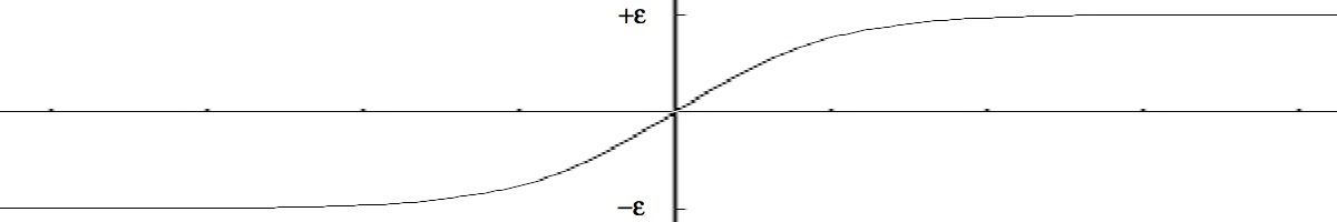
Figure 1: The integration contour $C_{+,\epsilon}$.

Notice that such imaginary Gaussian integrals oscillate, in contrast with the ordinary ones. They are not positive, hence in particular they are not probability measures. Also remark that although the result of integration does not depend on the contour, actual bounds on the result typically depend on choosing particular contours for which $\epsilon$ is not too small.

Remark also that if $f$ is a polynomial, the Gaussian rules of integration (found by Isserlis and called Wick theorem in physics) apply to such imaginary Gaussian integrals. More precisely, defining $(2n-1)!!:=(2n-1)(2n-3)\cdots 5.3.1$, we have

$$\int d\mu_{\pm iC}(x)x^{2n}=(\pm iC)^{n}(2n-1)!!\ .$$ (3)

This is easy to check since a polynomial is an entire function and we can deform the contour into $z=x+ix$, in which case we recover an ordinary Gaussian integration. Similarly

$$\int d\mu_{\pm iC}(x)e^{ax}=e^{\pm iCa^{2}/2},$$ (4)

the integral being absolutely convergent for any contour such that $C|a|<\epsilon$ .

We can also define imaginary complex normalized Gaussian integrals $d\mu^{c}_{\pm iC}(z)$ of covariance $\pm i$ for a complex variable $z$. This is in fact just the same as considering a pair of identical imaginary normalized Gaussian integrals of the previous type, one for the real part and the other for the imaginary part of $z$. Let us make this explicit. An ordinary complex Gaussian measure is usually written as

$$d\mu^{c}_{C}(z):=\frac{e^{-|z|^{2}/C}dzd\bar{z}}{\pi C}$$ (5)

so that

$$\int d\mu^{c}_{C}(z)z^{m}\bar{z}^{n}=\delta_{mn}C^{n}n!$$ (6)

What we call imaginary complex normalized Gaussian integrals $d\mu^{c}_{\pm iC}(z)$ are defined by writing $z=x+iy$ and separately writing two complex line integrals, one for $x$ and one for $y$. Let us rewrite a function $f(z)$ as a function of the real and imaginary parts of $z$ as $f(x+iy)=\phi(x,y)$. Assuming that $\phi$ admits an analytic continuation both in $x$ and $y$ in the product strip $\Im x\leq\delta,\Im y\leq\delta$ and is exponentially bounded in that domain by $Ke^{\eta(|x|+|y|)}$ for some $0\leq\eta<\delta$, where $K$ is some constant, we define

$$\int d\mu^{c}_{\pm iC}(z)f(z)=\frac{1}{\pm i\pi C}\int_{-\infty}^{+\infty}dx\int_{-\infty}^{+\infty}dye^{-[(x\pm i\epsilon\tanh x)^{2}+(y\pm i\epsilon\tanh y)^{2}]/\pm iC}\phi(x\pm i\epsilon\tanh x,y\pm i\epsilon\tanh y)$$ (7)

for which we have indeed the integration rules generalizing (5)-(6)

$$\int d\mu^{c}_{\pm iC}(z)z^{m}\bar{z}^{n}=\delta_{mn}(\pm iC)^{n}n!$$ (8)

and

$$\int d\mu^{c}_{\pm iC}(z)e^{az+b\bar{z}}=e^{\pm iabC},$$ (9)

again the last integral being absolutely convergent if $C\sup\{|a|,|b|\}<\epsilon$.

Following LR , we would also like to introduce some notations for pairs of imaginary Gaussian integrals with opposite imaginary covariances. More precisely suppose we have two variables $a$ and $b$, one with covariance $-i$ and the other $+i$ and corresponding integration contours in the complex plane of the type above. This integration being denoted as $d\mu_{\pm i}(a,b):=d\mu_{-i}(a)d\mu_{i}(b)$, we can perform the simple change of variables

$$\alpha=\frac{a+b}{\sqrt{2}},\qquad\qquad\beta=\frac{a-b}{\sqrt{2}},$$ (10)

and define the imaginary conjugate pair Gaussian integral $d\mu_{X}(\alpha,\beta)$ by its moments

$$<\alpha\beta>_{X}=-i,\ \ \quad<\alpha^{2}>_{X}=0,\ \ \quad<\beta^{2}>_{X}=0.$$ (11)

Hence this pair integral has two by two covariance $X=\begin{pmatrix}0&-i\\ -i&0\end{pmatrix}$. Remark that the two dimensional surface of integration in ${\mathbb{C}}^{2}$ remains defined by the one of the $a,b$ variables. Hence it is parametrized by $(\frac{\alpha+\beta}{\sqrt{2}},\frac{\alpha-\beta}{\sqrt{2}})\in C_{-,\epsilon}\times C_{+,\epsilon}$.

We should now define a more general class of Gaussian integrals combining a finite number of ordinary Gaussian measures and imaginary conjugate pair integrals.

Definition 2.

We call mixed Gaussian integral the product of finitely many ordinary real Gaussian measures and finitely many Gaussian imaginary conjugate pair integrals.

$$d\nu(\xi)=\prod_{i=1}^{p}d\mu_{1}(\sigma_{i})\prod_{j=1}^{q}d\mu_{X}(\alpha_{j},\beta_{j}).$$ (12)

We have a similar notion also for the complex integrals, which have twice as many real variables than the real ones.

Finally we can define such imaginary Gaussian measures for vectors, matrix or tensor variables $\vec{x}=(x_{1},\cdots x_{n})$ (real or complex) and a positive covariance matrix $C$ by deforming separately each integration contour for all real components, staying in the analyticity domain of the function $f$ where it remains exponentially bounded. For instance the imaginary Gaussian unitary ensemble with covariance $\pm i$ is defined as a product of normalized imaginary Gaussian integrals of covariance $\pm i$ on each of the $N^{2}$ real components $\{H_{ii},1\leq i\leq n,H_{ij},1\leq i<j\leq N\}$ of a Hermitian matrix $H$.

II.2 Borel-LeRoy-Nevanlinna-Sokal Theorem

We note $R^{q}f$ the $q$-th order Taylor remainder of a smooth function $f(\lambda)$. It writes

$$R^{q}f=\lambda^{q}\int_{0}^{1}\frac{(1-t)^{q-1}}{(q-1)!}f^{(q)}(t\lambda)dt.$$ (13)

Theorem 1.

(Borel-LeRoy-Nevanlinna-Sokal)

A power series $\sum_{n=0}^{\infty}\frac{a_{n}}{n!}\lambda^{n}$ is Borel-Le Roy summable of order $m$ to the function $f(\lambda)$ if the following conditions are met:

• For some real number $\rho>0$, $f(\lambda)$ is analytic in the domain $D^{m}_{\rho}=\{\lambda\in\mathbb{C}:\Re\lambda^{-1/m}>\rho^{-1}\}$.

• The function $f(\lambda)$ admits $\sum_{n=0}^{\infty}a_{n}\lambda^{n}$ as a strong asymptotic expansion to all orders as $|\lambda|$ $\rightarrow 0$ with uniform estimate in $D^{m}_{\rho}$:

  $$\left|R^{q}f\right|\leqslant AB^{q}\Gamma(mq)|\lambda|^{q}.$$ (14)

  where $A$ and $B$ are some constants and $\Gamma$ the usual Euler function.

Then the Borel-Le Roy transform of order $m$, which is

$$B^{(m)}_{f}(u)=\sum_{n=0}^{\infty}\frac{a_{n}}{\Gamma(mn+1)}u^{n},$$ (15)

is holomorphic for $|u|<B^{-1}$, it admits an analytic continuation to the strip $\{u\in\mathbb{C}:|\Im u|<R,\Re u>0\}$ for some $R>0$, and for $\lambda\in D^{m}_{\rho}$

$$f(\lambda)=\frac{1}{m\lambda}\int_{0}^{\infty}B^{(m)}_{f}(u)e^{-(\frac{u}{\lambda})^{\frac{1}{m}}}\bigl{(}\frac{u}{\lambda}\bigr{)}^{\frac{1}{m-1}}du.$$ (16)

For $m=1$ remark that $D^{1}_{\rho}$ is simply the usual disk of diameter $\rho$ tangent at the origin to the imaginary axis on the positive real part side of the complex plane. The proof of this theorem is a simple rewriting exercise on the usual Nevanlinna theorem Sok but in the variable $\lambda^{1/m}$.

III Matrix models

Definition 3.

We say that a function $Z$ has an Hermitian Intermediate Field (HIF) representation if it can be written as a convergent integral of the type

$$Z=\int d\nu(\xi)e^{-\operatorname{Tr}\ln\bigl{[}\mathds{1}-\mathbb{M}(\xi)\bigr{]}},$$ (17)

in which $d\nu(\xi)$ is a mixed Gaussian measure in the sense of the previous section, $\mathbb{M}(\xi)=iC\mathbb{H}(\xi)$, the matrix $\mathbb{H}$ is linear in term of all the $\xi$ variables, is Hermitian in term of their real parts (i.e. if we set $\epsilon=0$ in all contours), and $C$ is a mixed covariance, i.e. a sum of blocks made of diagonal 1 and finitely many $X=\begin{pmatrix}0&-i\\ -i&0\end{pmatrix}$ factors.

We consider now a complex, size-$N$, one-matrix model with $U(N)^{\otimes 2}$ invariant interaction of order $2k$, where $N\in\mathbb{N}^{\star}$. We always write $k-1=m$ in what follows since it will be the order of Borel summability to consider, and use the notation $O(1)$ for some constants independent of $N$ and $k$ whose exact values are not essential. The partition function of the model is

$$Z_{k}(\lambda,N):=\int d\mu^{c}(M)\exp\bigl{[}-\frac{\lambda}{N^{m}}\operatorname{Tr}(MM^{\dagger})^{k}\bigr{]},$$ (18)

where $d\mu^{c}$ is the normalized Gaussian measure $d\mu^{c}(M)=dMdM^{\dagger}e^{-\operatorname{Tr}MM^{\dagger}}$, $dMdM^{\dagger}=\pi^{-N^{2}}\prod_{i,j=1}^{N}dM_{ij}d\bar{M}_{ij}$. The associated free energy is

$$F_{k}(\lambda,N):=N^{-2}\log Z_{k}(\lambda,N).$$ (19)

It is a famous consequence of ’t Hooft $1/N$ expansion Hooft that the $N^{m}=N^{k-1}$ scaling in (18) is the correct one to ensure a non-trivial perturbative limit of $F_{k}(\lambda,N)$ when $N\to\infty$. More precisely with this particular scaling each (connected, vacuum) Feynman amplitude with $q$ vertices scales as $\lambda^{q}N^{-2g}$, where $g$ is the genus of the surface dual to the Feynman (ribbon) graph. Therefore in the sense of formal power series, $\lim_{N\to\infty}F_{k}(\lambda,N)=F_{k}^{planar}(\lambda)$ exists and is the generating function of planar ribbon graphs with (bipartite) vertices of degree $2k$ and coupling constant $\lambda$.

However it is much more difficult to perform the planar limit $\lim_{N\to\infty}F_{k}(\lambda,N)=F_{k}^{planar}(\lambda)$ not in the sense of formal power series but in a constructive sense, that is as a uniform limit of functions analytic in a well-defined domain. In the case of a quartic matrix interaction, the Loop Vertex Expansion which combines an intermediate field representation with a forest formula was introduced precisely to settle this issue Rivasseau:2007fr ; Gurau:2014lua . For instance it allows to prove the following:

Theorem 2.

There exist some $\rho>0$ such that all functions $F_{2}(\lambda,N)$ are analytic and Borel-summable (of ordinary order $m=1$) in $\lambda$ in an $N$-independent cardioid domain $Card_{\rho}$ defined in polar coordinates by $\lambda=\rho e^{i\phi}$, $\phi\in]-\pi,\pi[$ and $\rho<[\cos(\phi/2)]^{2}$. This domain is shown in Figure 2.

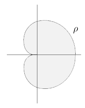
Figure 2: A cardioid domain

Furthermore in that domain the sequence $F_{2}(\lambda,N)$ uniformly converges as $N\to\infty$ to the function $F_{2}^{planar}(\lambda)$. This limit is not only Borel summable in $Card_{\rho}$ but also analytic in a disk centered at the origin containing $Card_{\rho}$.

The proof of this Theorem can be found in Gurau:2014lua . It states in particular that for $k=2$ the analyticity domain for $F_{2}(\lambda,N)$ does not shrink as $N\to\infty$.

However a constructive version of ‘t Hooft expansion remains to our knowledge a completely open issue in the case $k\geq 3$, hence for higher than quartic matrix trace interactions. We shall prove in this section the following result in this direction.

Theorem 3.

The partition function $Z_{k}(\lambda,N)$ and free energy $F_{k}(\lambda,N)$ are Borel-LeRoy summable of order $m=k-1$, in the sense of Theorem 1. More precisely they are analytic in $\lambda$ in the shrinking domain $D^{m}_{\rho_{m}(N)}=\{\lambda\in\mathbb{C}:\Re\lambda^{-1/m}>[\rho_{m}(N)]^{-1}\}$ with $\rho_{m}(N)=N^{-1-2/m}\rho_{m}$, $\rho_{m}>0$ independent of $N$. In that domain $Z_{k}(\lambda,N)$ has an HIF representation in the sense of Definition 3

$$Z_{k}(\lambda,N)=\int d\nu(\xi)e^{-N\operatorname{Tr}\ln\bigl{[}1-g_{k}\mathbb{M}_{k}(\xi)\bigr{]}},$$ (20)

in which

• the Gaussian measure $d\nu(\xi)$ is of the mixed Gaussian type in the sense of Definition 2

• $g_{k}=(\frac{\lambda}{N^{m}})^{\frac{1}{2k}}$,

• the matrix $\mathbb{M}_{k}(\xi)=iC_{k}.\mathbb{H}_{k}(\xi)$ is a $(k+1)N\times(k+1)N$ matrix,

• $C_{k}$ is a mixed covariance , i.e. a sum of blocks of type $\begin{pmatrix}1&0\\ 0&1\end{pmatrix}$ and $\begin{pmatrix}0&-i\\ -i&0\end{pmatrix}$ factors,

• $\mathbb{H}_{k}$ is linear in the $\{\xi\}$ variables and is Hermitian when these variables are taken on undeformed contours, i.e. at $\epsilon=0$.

This theorem is proven in the following subsections. We conjecture that for $k\geq 3$, just as for $k=2$, there should exist an analyticity domain common to all functions $Z_{k}(\lambda,N)$ and $F_{k}(\lambda,N)$ of the type $\{\lambda\in\mathbb{C}:\Re\lambda^{-1/m}>\rho^{-1}_{m}\}$ for some $\rho_{m}>0$ independent of $N$, hence which does not shrink as $N\to\infty$. However for the moment we do not know how to prove this stronger result, either using (18) or (20). We feel (20) may be a better starting point to attack this conjecture since in the case $k=2$, the only one in which the conjecture is proved, the proof uses such an intermediate field representation rather than the direct representation Rivasseau:2007fr ; Gurau:2014lua .

III.1 Formal intermediate field decomposition

To prove Theorem 3 let us first introduce the Hermitian intermediate field representation for $Z_{k}$, following the strategy of LR . This calls for a repetitive use of the Hubbard-Stratonovich decomposition applied to matrices

$$e^{-g\operatorname{Tr}(AB)}=\int d\mu^{c}(\tau)e^{i\sqrt{g}\,\operatorname{Tr}(A\tau+B\tau^{\dagger})},$$ (21)

and variations for intermediate fields of imaginary covariances $\pm i$

$$e^{ig\operatorname{Tr}(AB)}=\int d\mu^{c}_{\pm i}(\tau)e^{i\sqrt{g}\,\operatorname{Tr}(A\tau\mp B\tau^{\dagger})}.$$ (22)

Throughout this subsection we shall consider all Gaussian imaginary integrals in the $\epsilon\to 0$ formal limit. Therefore these integrals are not absolutely convergent, and the mathematically inclined reader may consider the computations of this subsection just as heuristic. However in the next subsection, the $\epsilon$ regulator will be reintroduced for all imaginary covariances, resulting in well defined convergent integrals confirming rigorously all these heuristic computations.

In all following sections, we shall use a graphical representation of the trace invariants in the action and of their iterated splittings. While it could seem a bit trivial in this section, it will prove very useful in the section treating tensorial invariants. We shall represent an integrated matrix $M$ by a white vertex and its complex conjugate by a black vertex. Edges between vertices carry a color, 1 or 2, and represent the contraction of the first or the second index between the two vertices. A matrix trace invariant of the form $\operatorname{Tr}((MM^{\dagger})^{k})$ is therefore pictured as a bipartite cycle, with alternating colors 1 and 2. This is shown in the $k=3$ case on the left of Figure 3,

Intermediate fields will be represented by black and white squares or triangles. As we shall see later, the associated graphs are not generally bipartite cycles of alternating colors.

Using relation (21), we first split the interaction term in two (Fig. 3), depending on the parity of $k$,

$$e^{-\frac{\lambda}{N^{k-1}}\operatorname{Tr}(MM^{\dagger})^{2p+1}} =\int d\mu^{c}(\sigma)e^{i\sqrt{\frac{\lambda}{N^{m}}}\operatorname{Tr}[(MM^{\dagger})^{p}(\sigma M^{\dagger}+M\sigma^{\dagger})]},$$ (23)

$$e^{-\frac{\lambda}{N^{k-1}}\operatorname{Tr}(MM^{\dagger})^{2p}} =\int d\mu^{c}(\sigma)e^{i\sqrt{\frac{\lambda}{N^{m}}}\operatorname{Tr}[(MM^{\dagger})^{p}(\sigma+\sigma^{\dagger})]}.$$ (24)

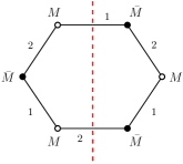
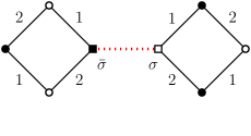
Figure 3: $k=3$ Matrix invariant and first intermediate field step.

Defining $g_{k}=(\frac{\lambda}{N^{k-1}})^{\frac{1}{2k}}$, we now rewrite the interactions as

$$\sqrt{\frac{\lambda}{N^{k-1}}}\operatorname{Tr}[(MM^{\dagger})^{p}(\sigma M^{\dagger}+M\sigma^{\dagger})] = \frac{1}{2}\operatorname{Tr}\bigl{[}((g_{k}^{2}MM^{\dagger})^{p}+g_{k}M\sigma^{\dagger})(g_{k}\sigma M^{\dagger}+(g_{k}^{2}MM^{\dagger})^{p})$$ (25)

$$\qquad+((g_{k}^{2}MM^{\dagger})^{p}-g_{k}M\sigma^{\dagger})(g_{k}\sigma M^{\dagger}-(g_{k}^{2}MM^{\dagger})^{p})\bigr{]},$$

$$\sqrt{\frac{\lambda}{N^{k-1}}}\operatorname{Tr}[(MM^{\dagger})^{p}(\sigma+\sigma^{\dagger})] = \frac{1}{2}\operatorname{Tr}\bigl{[}((g_{k}^{2}MM^{\dagger})^{p-1}M+g_{k}\sigma^{\dagger}M)(g_{k}M^{\dagger}\sigma+M^{\dagger}(g_{k}^{2}MM^{\dagger})^{p-1})$$

$$\qquad+((g_{k}^{2}MM^{\dagger})^{p-1}M-g_{k}\sigma^{\dagger}M)(g_{k}M^{\dagger}\sigma-M^{\dagger}(g_{k}^{2}MM^{\dagger})^{p-1})\bigr{]}.$$

Now applying (22) with complex intermediate fields $a_{1}$ and $b_{1}$ of covariances $-i$ and $+i$ respectively,

$$e^{-\frac{\lambda}{N^{k-1}}\operatorname{Tr}(MM^{\dagger})^{2p+1}} =\int d\mu^{c}(\sigma)d\mu^{c}_{\pm i}(a_{1},b_{1})e^{\frac{i}{\sqrt{2}}\operatorname{Tr}\bigl{[}(g_{k}^{2}MM^{\dagger})^{p}(a_{1}+b_{1}+a_{1}^{\dagger}+b_{1}^{\dagger})+g_{k}M\sigma^{\dagger}(a_{1}^{\dagger}-b_{1}^{\dagger})+g_{k}\sigma M^{\dagger}(a_{1}-b_{1})\bigr{]}}$$

$$e^{-\frac{\lambda}{N^{k-1}}\operatorname{Tr}(MM^{\dagger})^{2p}} =\int d\mu^{c}(\sigma)d\mu^{c}_{\pm i}(a_{1},b_{1})e^{\frac{i}{\sqrt{2}}\operatorname{Tr}\bigl{[}(g_{k}^{2}MM^{\dagger})^{p-1}(M(a_{1}^{\dagger}+b_{1}^{\dagger})+(a_{1}+b_{1})M^{\dagger})+g_{k}\sigma^{\dagger}M(a_{1}^{\dagger}-b_{1}^{\dagger})+g_{k}M^{\dagger}\sigma(a_{1}-b_{1})\bigr{]}},$$

where the measure is $d\mu^{c}_{\pm i}(a_{1},b_{1})=d\mu^{c}_{-i}(a_{1})d\mu^{c}_{+i}(b_{1})$.

Changing variables for

$$\alpha_{1}=\frac{a_{1}+b_{1}}{\sqrt{2}}\quad,\qquad\beta_{1}=\frac{a_{1}-b_{1}}{\sqrt{2}},$$ (27)

and complex conjugates, one finds that

$$e^{-\frac{\lambda}{N^{k-1}}\operatorname{Tr}(MM^{\dagger})^{2p+1}} =\int d\mu^{c}(\sigma)d\mu^{c}_{X}(\alpha_{1},\beta_{1})e^{i\operatorname{Tr}\bigl{[}(g_{k}^{2}MM^{\dagger})^{p}(\alpha_{1}+\alpha_{1}^{\dagger})+g_{k}M\sigma^{\dagger}\beta_{1}^{\dagger}+g_{k}\sigma M^{\dagger}\beta_{1}\bigr{]}}$$ (28)

$$e^{-\frac{\lambda}{N^{k-1}}\operatorname{Tr}(MM^{\dagger})^{2p}} =\int d\mu^{c}(\sigma)d\mu^{c}_{X}(\alpha_{1},\beta_{1})e^{i\operatorname{Tr}\bigl{[}(g_{k}^{2}MM^{\dagger})^{p-1}(\alpha_{1}M^{\dagger}+M\alpha_{1}^{\dagger})+g_{k}\sigma^{\dagger}M\beta_{1}^{\dagger}+g_{k}M^{\dagger}\sigma\beta_{1}\bigr{]}},$$

the Gaussian measure $d\mu^{c}_{X}$ being defined by its moments, that all vanish apart from

$$\forall j,k\in\{1,...,N\},\quad<\alpha_{1\mid jk}\bar{\beta}_{1\mid jk}>_{X}=<\bar{\alpha}_{1\mid jk}\beta_{1\mid jk}>_{X}=-i.$$ (29)

Inductively applying the same reasoning leads to the following expressions for the partition function,

$$Z_{k,odd}(\lambda,N) = \int d\mu^{c}(\phi)d\mu^{c}(\sigma)\prod_{j=1}^{k-2}d\mu^{c}_{X}(\alpha_{j},\beta_{j})e^{ig_{k}\operatorname{Tr}\bigl{[}M^{\dagger}\bigl{(}\beta_{1}\sigma+\alpha_{1}\beta_{2}+\beta_{3}\alpha_{2}+\cdots+\beta_{k-2}\alpha_{k-3}+g_{k}\alpha_{k-2}M\bigr{)}+\,c.t.\bigr{]}},$$

$$Z_{k,even}(\lambda,N) = \int d\mu^{c}(\phi)d\mu^{c}(\sigma)\prod_{j=1}^{k-2}d\mu^{c}_{X}(\alpha_{j},\beta_{j})e^{ig_{k}\operatorname{Tr}\bigl{[}M^{\dagger}\bigl{(}\sigma\beta_{1}+\beta_{2}\alpha_{1}+\alpha_{2}\beta_{3}+\cdots+\beta_{k-2}\alpha_{k-3}+g_{k}\alpha_{k-2}M\bigr{)}+\,c.t.\bigr{]}},$$ (30)

where $c.t.$ stands for conjugate transpose. The $i$’th splitting introduces the matrix intermediate fields $\alpha_{i+1}$ and $\beta_{i+1}$, with complex covariances as in (29) (respectively represented by a square vertex and a triangle vertex) and is represented in Figure 4 (this may also apply for $\alpha_{0}=\sigma$). Note that the graphs representing the interactions have plain lines.

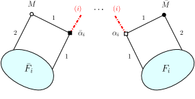
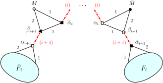
Figure 4: Step $i$ of the intermediate field decomposition, when $F_{i}$ has an odd number of vertices. In the even case, the edge between $M$ and $\bar{\alpha}_{i}$ and symmetric are of color 2, while the edges toward $F_{i}$ are both of color 1.

The partition function rewrites in both cases as

$$Z_{k}(\lambda,N)=\int d\mu^{c}(M)d\mu^{c}(\sigma)\prod_{j=1}^{k-2}d\mu^{c}_{X}(\alpha_{j},\beta_{j})e^{ig_{k}\operatorname{Tr}\bigl{[}M^{\dagger}R_{k}+R_{k}^{\dagger}M\bigr{]}},$$ (31)

where, defining $\alpha_{0}:=\sigma$, $\beta_{k-1}:=M$ and $\beta_{0}=\alpha_{-1}=0$,

$$R_{k}(\sigma,\{\alpha_{j},\beta_{j}\})=\sum_{j=1}^{\lfloor\frac{k}{2}\rfloor}(\alpha_{k-2j}\beta_{k-2j+1}+\beta_{k-2j}\alpha_{k-2j-1}),$$ (32)

We now integrate over a subset of the intermediate fields using relation

$$\int d\mu^{c}_{X}(\alpha,\beta)e^{i\operatorname{Tr}[A\alpha+B\beta+C\alpha^{\dagger}+D\beta^{\dagger}]}=e^{i\operatorname{Tr}[AD+BC]}.$$ (33)

We choose to integrate over $M$ and all $\alpha_{k-1-2j}$, $\beta_{k-1-2j}$, for $j\in\{0,...,\lfloor\frac{k}{2}\rfloor\}$, i.e.

• for $k$ odd, over the $k-1$ matrix fields $M$, $\sigma$ and all even $\alpha_{2j}$, $\beta_{2j}$, for $j\in\{1,..,\frac{k-3}{2}\}$ and complex conjugates.

• for $k$ even, over the $k-1$ matrix fields $M$ and all odd $\alpha_{2j-1}$, $\beta_{2j-1}$, for $j\in\{1,..,\frac{k-2}{2}\}$ and complex conjugates.

Each integration step is done independently of the others. It gives

$$\int d\mu^{c}_{X}(\alpha_{k-1-2j},\beta_{k-1-2j})e^{ig_{k}\operatorname{Tr}\bigl{[}M^{\dagger}(\beta_{k-2j}\alpha_{k-1-2j}+\alpha_{k-2(j+1)}\beta_{k-1-2j})+c.t.\bigr{]}}=\ e^{ig_{k}^{2}\operatorname{Tr}\bigl{[}M^{\dagger}\beta_{k-2j}\alpha_{k-2(j+1)}^{\dagger}M+c.t.\bigr{]}},$$ (34)

except for the $\sigma$ integration for $k$ odd, which gives

$$\int d\mu^{c}(\sigma)e^{ig_{k}\operatorname{Tr}\bigl{[}M^{\dagger}\beta_{1}\sigma+c.t.\bigr{]}}=\ e^{-g_{k}^{2}\operatorname{Tr}\bigl{[}M^{\dagger}\beta_{1}\beta_{1}^{\dagger}M\bigr{]}}.\$$ (35)

Let $\xi=(...\alpha_{k-2j},\beta_{k-2j},...)$ be the vector containing the $k-1$ remaining variables, $\xi_{odd}=(\alpha_{1},\beta_{1},...,\alpha_{k-2},\beta_{k-2})$ and $\xi_{even}=(\sigma,\alpha_{2},\beta_{2},...,\alpha_{k-2},\beta_{k-2})$. Note that the indices of the remaining intermediate fields have the parity of $k$. The partition function therefore rewrites

$$Z_{k}(\lambda,N)=\int d\nu(\xi)e^{-N\operatorname{Tr}\ln\bigl{[}\mathds{1}-g_{k}^{2}\bigl{(}iH_{k}(\xi)-\eta(k)\beta_{1}\beta_{1}^{\dagger}\bigr{)}\ \bigr{]}},$$ (36)

where ${\mathds{1}}$ is the $N$ by $N$ identity matrix, $d\nu$ factorizes over the measures $d\mu_{X}^{c}$ of each $\alpha,\beta$ pair plus the measure $d\mu^{c}(\sigma)$ for $k$ even, and $\eta(k)$ is 0 for $k$ even and 1 for $k$ odd, and where we denoted $H_{k}$ the $N\times N$ Hermitian matrix

$$H_{k}(\xi)=\sum_{j=0}^{\lfloor\frac{k}{2}\rfloor}\beta_{k-2j}\alpha_{k-2(j+1)}^{\dagger}+c.t.\ .$$ (37)

The detailed graphical representation of the successive intermediate field splittings is summarized in Figures 5 and 6 for the $k=4$ case.

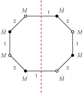
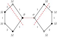
Figure 5: $k=4$ matrix trace invariant and initial intermediate field step.

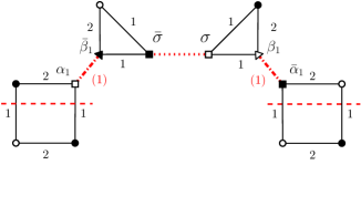
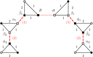
Figure 6: Successive intermediate field splittings for matrices

Hermitian Intermediate Field Representation

Expression (36) can be reformulated using a $(k+1)N\times(k+1)N$ determinant

$$Z_{k}(\lambda,N)=\int d\nu(\xi)e^{-N\operatorname{Tr}\ln\bigl{[}{\mathds{1}}^{\otimes(k+1)}-g_{k}\mathbb{M}_{k}(\xi)\bigr{]}},$$ (38)

where $\mathbb{M}_{k}(\xi)=iC_{k}.\mathbb{H}_{k}(\xi)$, $C_{k}$ is the complex symmetric covariance of the integrated fields

$$C_{odd}=\left(\begin{array}[]{ccccccc}{\mathds{1}}&\lx@intercol\hfil 0\hfil\lx@intercol\vrule\lx@intercol&&&&&\\ 0&\lx@intercol\hfil{\mathds{1}}\hfil\lx@intercol\vrule\lx@intercol&&&&&\\ \cline{1-4}\cr&\lx@intercol\hfil\hfil\lx@intercol\vrule\lx@intercol&0&\lx@intercol\hfil-i{\mathds{1}}\hfil\lx@intercol\vrule\lx@intercol&&\Large\mbox{{$0$}}&\\ &\lx@intercol\hfil\hfil\lx@intercol\vrule\lx@intercol&-i{\mathds{1}}&\lx@intercol\hfil 0\hfil\lx@intercol\vrule\lx@intercol&&&\\ \cline{3-6}\cr&&&\lx@intercol\hfil\hfil\lx@intercol\vrule\lx@intercol&0&\lx@intercol\hfil-i{\mathds{1}}\hfil\lx@intercol\vrule\lx@intercol&\\ &&\Large\mbox{{$0$}}&\lx@intercol\hfil\hfil\lx@intercol\vrule\lx@intercol&-i{\mathds{1}}&\lx@intercol\hfil 0\hfil\lx@intercol\vrule\lx@intercol&\\ \cline{5-6}\cr&&&&&&\ddots\end{array}\right),\quad C_{even}=\left(\begin{array}[]{cccccc}\lx@intercol\hfil{\mathds{1}}\hfil\lx@intercol\vrule\lx@intercol&&&&&\\ \cline{1-3}\cr\lx@intercol\hfil\hfil\lx@intercol\vrule\lx@intercol&0&\lx@intercol\hfil-i{\mathds{1}}\hfil\lx@intercol\vrule\lx@intercol&&\Large\mbox{{$0$}}&\\ \lx@intercol\hfil\hfil\lx@intercol\vrule\lx@intercol&-i{\mathds{1}}&\lx@intercol\hfil 0\hfil\lx@intercol\vrule\lx@intercol&&&\\ \cline{2-5}\cr&&\lx@intercol\hfil\hfil\lx@intercol\vrule\lx@intercol&0&\lx@intercol\hfil-i{\mathds{1}}\hfil\lx@intercol\vrule\lx@intercol&\\ &\Large\mbox{{$0$}}&\lx@intercol\hfil\hfil\lx@intercol\vrule\lx@intercol&-i{\mathds{1}}&\lx@intercol\hfil 0\hfil\lx@intercol\vrule\lx@intercol&\\ \cline{4-5}\cr&&&&&\ddots\end{array}\right).$$ (52)

The matrix $\mathbb{H}_{k}$ is Hermitian, and has two different forms depending whether $k$ is odd or even

$$\mathbb{H}^{odd}_{k}=\left(\begin{array}[]{c|ccccc}0&\beta_{1}&\alpha_{1}&\cdots&\alpha_{k-2}&{\mathds{1}}\\ \hline\cr\beta_{1}^{\dagger}&&&\raisebox{-30.0pt}{{\huge\mbox{{$0$}}}}\\[-25.83325pt] \alpha_{1}^{\dagger}&\\[-2.15277pt] \vdots&\\[-2.15277pt] \alpha_{k-2}^{\dagger}&\\ {\mathds{1}}&\\[-2.15277pt] \end{array}\right),\quad\mathbb{H}^{even}_{k}=\left(\begin{array}[]{c|ccccc}0&\sigma&\beta_{2}&\cdots&\alpha_{k-2}&{\mathds{1}}\\ \hline\cr\sigma^{\dagger}&&&\raisebox{-30.0pt}{{\huge\mbox{{$0$}}}}\\[-25.83325pt] \beta_{2}^{\dagger}&\\[-2.15277pt] \vdots&\\[-2.15277pt] \alpha_{k-2}^{\dagger}&\\ {\mathds{1}}&\\[-2.15277pt] \end{array}\right).$$ (53)

Therefore we have explicitly

$$\mathbb{M}^{odd}_{k}=\left(\begin{array}[]{c|ccccc}0&i\beta_{1}&i\alpha_{1}&\cdots&i\alpha_{k-2}&i{\mathds{1}}\\ \hline\cr i\beta_{1}^{\dagger}&&&\raisebox{-30.0pt}{{\huge\mbox{{$0$}}}}\\[-25.83325pt] \beta_{3}^{\dagger}&\\[-2.15277pt] \vdots&\\[-2.15277pt] {\mathds{1}}&\\ \alpha_{k-2}^{\dagger}&\\[-2.15277pt] \end{array}\right),\quad\mathbb{M}^{even}_{k}=\left(\begin{array}[]{c|ccccc}0&i\sigma&i\beta_{2}&\cdots&i\alpha_{k-2}&i{\mathds{1}}\\ \hline\cr\beta_{2}^{\dagger}&&&\raisebox{-30.0pt}{{\huge\mbox{{$0$}}}}\\[-25.83325pt] \sigma^{\dagger}&\\[-2.15277pt] \vdots&\\[-2.15277pt] {\mathds{1}}&\\ \alpha_{k-2}^{\dagger}&\\[-2.15277pt] \end{array}\right).$$ (54)

Examples. In the simplest cases $k=3,4$, hence the $e^{-\frac{\lambda}{N^{2}}\operatorname{Tr}[(MM^{\dagger})^{3}]}$ and $e^{-\frac{\lambda}{N^{3}}\operatorname{Tr}[(MM^{\dagger})^{4}]}$ models, we obtain the representations:

$$Z_{3}(\lambda,N)=\int d\mu_{X}^{c}(\alpha_{1},\beta_{1})e^{-N\operatorname{Tr}\ln\bigl{[}{\mathds{1}}^{\otimes 4}-g_{3}\mathbb{M}_{3}(\alpha_{1},\beta_{1})\bigr{]}},\quad g_{3}=\frac{\lambda^{1/6}}{N^{1/3}},\quad\mathbb{M}_{3}=\begin{pmatrix}0&i\beta_{1}&i\alpha_{1}&i{\mathds{1}}\\ i\beta_{1}^{\dagger}&0&0&0\\ \mathds{1}&0&0&0\\ \alpha_{1}^{\dagger}&0&0&0\end{pmatrix}$$ (55)

and

$$Z_{4}(\lambda,N)=\int d\mu^{c}(\sigma)d\mu_{X}^{c}(\alpha_{2},\beta_{2})e^{-N\operatorname{Tr}\ln\bigl{[}{\mathds{1}}^{\otimes 5}-g_{4}\mathbb{M}_{4}(\alpha_{2},\beta_{2})\bigr{]}},\quad g_{4}=\frac{\lambda^{1/8}}{N^{3/8}},\quad\mathbb{M}_{4}=\begin{pmatrix}0&i\sigma&i\beta_{2}&i\alpha_{2}&i\mathds{1}\\ \beta_{2}^{\dagger}&0&0&0&0\\ \sigma\dagger&0&0&0&0\\ \mathds{1}&0&0&0&0\\ \alpha_{2}\dagger&0&0&0&0\end{pmatrix}.$$ (56)

III.2 Analyticity Domain and Borel Summability

Our main task in this subsection is to complete the proof of Theorem 3. We still have to prove

Theorem 4.

For any fixed $N$ the normalization $Z_{k}(\lambda,N)$ and the free energy $F_{k}:=N^{-2}\log Z_{k}(\lambda,N)$ are Borel-Le Roy summable of order $m=k-1$, in the shrinking domain $D^{m}_{\rho_{m}(N)}$ with $\rho_{m}(N)=N^{-1-2/m}r_{m}$, $r_{m}>0$ independent of $N$.

We shall in fact prove analyticity and uniform Taylor remainder estimates in a slightly larger (but similarly shrinking as $N\to\infty$) domain $E^{m}_{\rho_{m}(N)}$ consisting of all $\lambda$’s with $|\lambda|<[\rho_{m}(N)]^{m}$, and $|\arg\lambda|<\frac{m\pi}{2}$, hence for $\lambda^{1/m}$ in an open half-disk of radius $\rho_{m}(N)$, which obviously contains the smaller tangent disk $D^{m}_{\rho_{m}(N)}$ of diameter $\rho_{m}(N)$ necessary for Theorem 1.

Our strategy is to bound the determinant factor $e^{-N\operatorname{Tr}\ln\bigl{[}{\mathds{1}}^{\otimes(k+1)}-g_{k}\mathbb{M}_{k}(\xi)\bigr{]}}$ in the Hermitian representation (38) by computing the eigenvalues of the matrix ${\mathds{1}}^{\otimes(k+1)}-g_{k}\mathbb{M}_{k}$. In order to have absolutely convergent formulas instead of formal expressions we need however to now reinstall everywhere the correct contour integrals with the $\epsilon$ regulator. It means that in every integral over $\alpha$ and $\beta$ variables we have to return to the $a+b$ or $a-b$ real and imaginary parts, which we call collectively the $\{a,b\}$ variables. Instead of being formally integrated each over the real line with an oscillating factor $e^{-ia^{2}}$ or $e^{+ib^{2}}$, we need to integrate each such $a$ or $b$ variable with the appropriate $C_{\pm\epsilon}$ contour. This is equivalent to keep every $a$ or $b$ contour real but then first substitute $a\to a-i\epsilon\tanh a$ and $b\to b+i\epsilon\tanh b$ into all imaginary factors $e^{-ia^{2}}$ and $e^{+ib^{2}}$, and second perform the same substitution into all $a$ and $b$ linear-dependent coefficients of $\mathbb{M}_{k}(\{a,b\})$. Remark that this destroys the Hermitian character of the matrix $H_{k}$. More precisely since the $\mathbb{M}_{k}$ matrix depends linearly of all $\{a,b\}$ variables, this second substitution corresponds to substitute

$$\mathbb{M}_{k}(\{a,b\})\to\mathbb{M}_{k}(\{a,b\})+\epsilon\mathbb{N}_{k}(\{a,b\})$$ (57)

where $\mathbb{N}_{k}$ is $(k+1)N\times(k+1)N$ with matrix elements all zero except on the first $N$ rows and first $N$ columns. In these rows and columns, remark that any non zero matrix element is of the form $\pm(i)\frac{1}{\sqrt{2}}(\tanh a_{jk}\pm\tanh b_{jk})$ for some $j,k$ where the factor $i$ may or may not be present. Hence

Lemma 1.

The operator norm of $\mathbb{N}_{k}$ is uniformly bounded by $2\sqrt{k}N$, hence

$$\|\epsilon g_{k}\mathbb{N}_{k}(\{a,b\})\|\leq 2\epsilon|g_{k}|\sqrt{k}N\quad\quad\forall\{a,b\}.$$ (58)

Proof    Simply bound $\|\mathbb{N}_{k}\|$ by its Hilbert-Schmidt norm $\|\mathbb{N}_{k}\|_{2}$ (we took into account that the first $N$ by $N$ block in $\mathbb{N}_{k}$ is zero). ∎

Returning to the $\mathbb{M}_{k}(\{a,b\})$ matrix, we now study its spectrum by computing its characteristic polynomial in term of the Hermitian matrix $H_{k}$.

Lemma 2.

Considering $\mathbb{M}_{k}$, $H_{k}$ and $\eta(k)$ as defined before, the characteristic polynomial of the $(k+1)N\times(k+1)N$ matrix ${\mathds{1}}^{\otimes(k+1)}-g_{k}\mathbb{M}_{k}$ is

$$\det[(1-x){\mathds{1}}^{\otimes(k+1)}-g_{k}\mathbb{M}_{k}]\ =\ (1-x)^{(k-1)N}\det[(1-x)^{2}{\mathds{1}}_{N}-g_{k}^{2}(iH_{k}-\eta(k)\beta_{1}\beta_{1}^{\dagger})]$$ (59)

Proof    It follows from the $(k+1)N\times(k+1)N$ square matrix identity

$$\left(\begin{array}[]{c|c|c|c}(1-x)^{2}\mathds{1}&-g_{k}A_{1}&\cdots&-g_{k}A_{k}\\[4.30554pt] \hline\cr-(1-x)g_{k}B_{1}&(1-x)\mathds{1}&0&0\\[4.30554pt] \hline\cr\vdots&0&\ddots&\vdots\\[4.30554pt] \hline\cr-(1-x)g_{k}B_{k}&0&\cdots&(1-x)\mathds{1}\\[4.30554pt] \hline\cr\end{array}\right)=\left(\begin{array}[]{c|c|c|c}U&-g_{k}A_{1}&\cdots&-g_{k}A_{k}\\[4.30554pt] \hline\cr 0&(1-x)\mathds{1}&0&0\\[4.30554pt] \hline\cr\vdots&0&\ddots&\vdots\\[4.30554pt] \hline\cr 0&0&\cdots&(1-x)\mathds{1}\\[4.30554pt] \end{array}\right)\left(\begin{array}[]{c|c|c|c}\mathds{1}&\quad 0&\cdots&\quad 0\\[4.30554pt] \hline\cr-g_{k}B_{1}&\mathds{1}&0&0\\[4.30554pt] \hline\cr\vdots&0&\ddots&\vdots\\[4.30554pt] \hline\cr-g_{k}B_{k}&0&\cdots&\mathds{1}\\[4.30554pt] \end{array}\right),$$

where $U=(1-x)^{2}\mathds{1}-g_{k}^{2}\sum_{j=1}^{k}A_{j}B_{j}$. Choosing $0,A_{1},\cdots,A_{k}$, as the first row of $\mathbb{M}_{k}$ and $0,B_{1},\cdots,B_{k}$ as the first column of $\mathbb{M}_{k}$, and taking the determinant of this identity, one obtains that

$$(1-x)\det[(1-x){\mathds{1}}^{\otimes(k+1)}-g_{k}\mathbb{M}_{k}]=\det(U)(1-x)^{kN},$$ (60)

so that

$$\det[(1-x){\mathds{1}}^{\otimes(k+1)}-g_{k}\mathbb{M}_{k}]=\det(U)(1-x)^{(k-1)N}.$$ (61)

More precisely, for $k$ odd we choose $A_{1}=i\beta_{1}$, $A_{2}=i\alpha_{1}$, …$A_{k-1}=i\alpha_{k-2}$, $A_{k}=i\mathds{1}$ and $B_{1}=i\beta_{1}^{\dagger}$, $B_{2}=\beta_{3}^{\dagger}$, …$B_{k-1}=\mathds{1}$, $B_{k}=\alpha_{k-2}^{\dagger}$, and for $k$ even we choose $A_{1}=i\sigma$, $A_{2}=i\beta_{2}$, …$A_{k-1}=i\alpha_{k-2}$, $A_{k}=i\mathds{1}$ and $B_{1}=\beta_{2}^{\dagger}$, $B_{2}=\sigma^{\dagger}$, …$B_{k-1}=\mathds{1}$, $B_{k}=\alpha_{k-2}^{\dagger}$. In all cases we find

$$U=(1-x)^{2}\mathds{1}-g_{k}^{2}\sum_{j=1}^{k}A_{j}B_{j}=(1-x)^{2}\mathds{1}-g_{k}^{2}[iH_{k}-\eta(k)\beta_{1}\beta_{1}^{\dagger}].$$ (62)

∎

To prove Borel-Le Roy summability of order $m$ of $Z_{k}$ and $\log Z_{k}$ of order $m=k-1$ in the intermediate field representation (38) the key step is an upper bound on the norm of the resolvent $[1-g_{k}\mathbb{M}_{k}(\{a,b\})]^{-1}$. This bound must be uniform both in $\lambda$ in that domain and uniform in the intermediate fields along the contours.

Lemma 3.

For $\lambda\in E^{m}_{\rho_{m}(N)}$ we have

$$\|({\mathds{1}}^{\otimes(k+1)}-g_{k}\mathbb{M}_{k})^{-1}\|\leq[\sin\frac{\pi}{4k}]^{-1}.$$ (63)

Proof    Let us compute the spectrum of the matrix ${\mathds{1}}^{\otimes(k+1)}-g_{k}\mathbb{M}_{k}(\{a,b\})$. By the previous Lemma it has a trivial eigenvalue $1$ with multiplicity $N(k-1)$ and an additional non trivial spectrum, which is exactly made of the elements $x$ of the form $x=1\pm g_{k}\sqrt{y}$ where $y$ belongs to the spectrum of the matrix $iH_{k}-\eta(k)\beta_{1}\beta_{1}^{\dagger}$. But $y$ belongs to the spectrum of that matrix if and only if

$$\det(-y+iH_{k}-\eta(k)\beta_{1}\beta_{1}^{\dagger})=0.$$ (64)

This is equivalent to the existence of an eigenvector $u$ with $\|u\|=1$ such that $(-y+iH_{k}-\eta(k)\beta_{1}\beta_{1}^{\dagger})u=0$, hence for which $y=-\eta(k)\|\beta_{1}^{\dagger}u\|^{2}+i<u,H_{k}u>$. Hence, since $H_{k}$ is Hermitian, no matter whether $\eta(k)=0$ or 1, $y$ must be of the form $-v^{2}+iw$ with $v$ and $w$ real. It means that any square root of $y$ (written as $\pm\sqrt{y}$) must be either 0 or have a complex argument in $I=[\frac{\pi}{4},\frac{3\pi}{4}]\cup[-\frac{3\pi}{4},-\frac{\pi}{4}]$. But in the domain $E^{k}_{\rho}$ the argument of $g_{k}$ is bounded by $\frac{(k-1)\pi}{4k}$ hence the argument of $\pm g_{k}\sqrt{y}$ (when $y\neq 0$) must lie in

$$I_{k} = [\frac{\pi}{4}-\frac{(k-1)\pi}{4k},\frac{3\pi}{4}+\frac{(k-1)\pi}{4k}]\cup[-\frac{3\pi}{4}-\frac{(k-1)\pi}{4k},-\frac{\pi}{4}+\frac{(k-1)\pi}{4k}]$$ (65)

$$= [\frac{\pi}{4k},\pi-\frac{\pi}{4k}]\cup[-\pi+\frac{\pi}{4k},-\frac{\pi}{4k}],$$

hence in that domain the spectrum of ${\mathds{1}}^{\otimes(k+1)}-g_{k}\mathbb{M}_{k}$ lies out of the open disk of center 0 and radius $\sin\frac{\pi}{4k}$. ∎

We denote $R_{k}=r_{m}^{\frac{m}{2k}}=r_{k-1}^{\frac{k-1}{2k}}$.

Lemma 4.

For $\lambda\in E^{m}_{\rho_{m}(N)}$, choosing $\epsilon=R_{k}^{-1}\frac{\sin(\pi/4k)}{4\sqrt{k}}$ we have

$$\|[{\mathds{1}}^{\otimes(k+1)}-g_{k}(\mathbb{M}_{k}+\epsilon\mathbb{N}_{k})]^{-1}\|\leq 2[\sin\frac{\pi}{4k}]^{-1}.$$ (66)

Proof    We recall that for $\lambda\in E^{m}_{\rho_{m}(N)}$, $|\lambda|\leq\rho_{m}(N)^{m}$. Since $\rho_{m}(N)=N^{-1-\frac{2}{m}}r_{m}$, it implies

$$|g_{k}|=|\lambda|^{\frac{1}{2k}}N^{-\frac{m}{2k}}\leq\rho_{m}(N)^{\frac{m}{2k}}N^{-\frac{m}{2k}}=N^{-\frac{m}{2k}-\frac{1}{k}}N^{-\frac{m}{2k}}r_{m}^{\frac{m}{2k}}=N^{-\frac{m}{k}-\frac{1}{k}}R_{k}=N^{-1}R_{k}.$$ (67)

Hence by Lemma 1 we have $\|\epsilon g_{k}\mathbb{N}_{k}\|\leq\frac{1}{2}\sin\frac{\pi}{4k}$. Since

$$[{\mathds{1}}^{\otimes(k+1)}-g_{k}(\mathbb{M}_{k}+\epsilon\mathbb{N}_{k})]^{-1}=[{\mathds{1}}^{\otimes(k+1)}-({\mathds{1}}^{\otimes(k+1)}-g_{k}\mathbb{M}_{k})^{-1}g_{k}\epsilon\mathbb{N}_{k}]^{-1}({\mathds{1}}^{\otimes(k+1)}-g_{k}\mathbb{M}_{k})^{-1},$$ (68)

it implies

$$\|[{\mathds{1}}^{\otimes(k+1)}-g_{k}(\mathbb{M}_{k}+\epsilon\mathbb{N}_{k})]^{-1}\|\leq\bigl{(}1-[\sin\frac{\pi}{4k}]^{-1}\frac{1}{2}\sin\frac{\pi}{4k}\bigr{)}^{-1}[\sin\frac{\pi}{4k}]^{-1}=2[\sin\frac{\pi}{4k}]^{-1}.$$ (69)

∎

Remark that this bound also implies a bound on the factor $e^{-N\operatorname{Tr}\ln\bigl{[}{\mathds{1}}^{\otimes(k+1)}-g_{k}(\mathbb{M}_{k}+\epsilon\mathbb{N}_{k})(\xi)\bigr{]}}$ in (38), namely

$$e^{-N\operatorname{Tr}\ln\bigl{[}{\mathds{1}}^{\otimes(k+1)}-g_{k}(\mathbb{M}_{k}+\epsilon\mathbb{N}_{k})(\xi)\bigr{]}}=|{\rm det}^{-N}[{\mathds{1}}^{\otimes(k+1)}-g_{k}(\mathbb{M}_{k}+\epsilon\mathbb{N}_{k})]|\leq e^{2N^{2}|\log\frac{\sin\frac{\pi}{4k}}{2}|}=2^{2N^{2}}[\sin\frac{\pi}{4k}]^{-2N^{2}},$$ (70)

since there are only at most $2N$ non zero eigenvalues of $\mathbb{M}_{k}+\epsilon\mathbb{N}_{k}$. It means a uniform upper bound on the integrand in (38). Since the integration in $d\nu$ is over $2(k-1)N^{2}$ integration contours, taking absolute values for each of them with $\epsilon=R_{k}^{-1}\frac{\sin(\pi/4k)}{4\sqrt{k}}$ leads to a loss of $O(1)k^{3/2}$ per contour. Hence since $[\sin\frac{\pi}{4k}]^{-1}\leq O(1)k$ in the shrinking domain we have the uniform bound

$$|Z_{k}(\lambda,N)|\leq O(1)^{k^{3/2}N^{2}}\quad\implies\quad|F_{k}(\lambda,N)|\leq O(1)^{k^{3/2}}.$$ (71)

Analyticity of $Z_{k}$ and $F_{k}$ (for any finite $N$, but non-uniformly in $N$) then follows by the standard theorem that a uniformly convergent integral of an analytic integrand is analytic.

For any finite $N$ the perturbation theory of $Z_{k}$ in the intermediate field representation is identical to the standard one in the direct representation (this just follows from the fact that they are independent of the $\epsilon$ regulator, see (8)). As usual, Borel-LeRoy Taylor remainder bounds just correspond to the factorial growth of perturbation theory and follow easily. Indeed they correspond to insert $q$ additional vertices (with a $1/q!$ symmetry factor) in the functional integral for $Z$, hence $qk$ pairs of fields. It is by now well known that this adds simply $qk$ resolvents to the functional integral Gurau:2013pca , together with a factor $(qk)!$ for pairing the arguments into the resolvents. But since our bounds for the determinant in $Z$ precisely followed from a uniform bound on such resolvents (Lemma 4), we obtain a bound in $O(1)^{kq}$ for addition of such resolvents. Combining the two factorials leads to a bound in $[O(1)|\lambda|]^{q}\frac{qk!}{q!}$, hence since $m=k-1$, this bound is exactly of the desired type (14).

By unicity of the Borel sum, we can claim that representation (38), although derived by some formal computations at $\epsilon=0$, is in fact convergent when $\epsilon$-dependent contours are used, and that it defines non-perturbatively the same partition function and free energy that the direct initial representation. These results extend easily to free energy with sources, hence to cumulants of the theory.

IV Positive tensor models

IV.1 Random tensor models

We include here for self-containedness a brief remainder about invariant (uncolored) tensor models, essentially reproduced from Bonzom:2012hw .

Let ${\cal{H}}_{1},\dotsc,{\cal{H}}_{D}$ be complex Hilbert spaces of dimensions $N_{1},\dotsc,N_{D}$. A rank $D$ covariant tensor $T_{n_{1}\dotsc n_{D}}$ is a collection of $\prod_{i=1}^{D}N_{i}$ complex numbers supplemented with the requirement of covariance under independent change of basis in each ${\cal{H}}_{i}$. The complex conjugate tensor $\bar{T}_{n_{1}\dotsc n_{D}}$ is then a rank $D$ contravariant tensor. Under independent unitary base change $U^{(i)}$ in each $U(N_{i})$, $T$ and $\bar{T}$ transform as

$$T^{\prime}_{a_{1}\dotsc a_{D}}=\sum_{n_{1},\dotsc,n_{D}}U^{(1)}_{a_{1}n_{1}}\dotsm U^{(D)}_{a_{D}n_{D}}\ T_{n_{1}\dotsc n_{D}}\;,\qquad\bar{T}^{\prime}_{a_{1}\dots a_{D}}=\sum_{n_{1},\dotsc,n_{D}}\bar{U}^{(D)}_{a_{D}n_{D}}\dotsm\bar{U}^{(1)}_{a_{1}n_{1}}\ \bar{T}_{n_{1}\dots n_{D}}\;.$$ (72)

From now on we shall restrict to the case where all $N_{i}$, $i=1,\cdots D$ are equal to $N$. A trace invariant is a connected monomial in $T$ and $\bar{T}$ invariant under that action of the external tensor product of the $D$ independent unitary groups $U(N)$, namely $U(N)^{\otimes D}$. It is built by contracting all tensor indices two by two, a tensor entry always with a conjugate tensor entry, respecting the positions of indices. Note that a trace invariant has necessarily the same number of $T$ and $\bar{T}$. Any trace invariant is then represented by a $D$-bubble, which is a D-regular edge-colored bipartite graph:

Definition 4.

A closed $D$-colored graph, or $D$-bubble, is a connected graph $\mathcal{B}=(\mathcal{V},\mathcal{E})$ with vertex set $\mathcal{V}$ and line set $\mathcal{E}$ such that

• $\mathcal{V}$ is bipartite, i.e. there exists a partition of the vertex set $\mathcal{V}=A\cup\bar{A}$, such that for any element $l\in\mathcal{E}$, then $l=\{v,\bar{v}\}$ with $v\in A$ and $\bar{v}\in\bar{A}$. Their cardinalities satisfy $|\mathcal{V}|=2|A|=2|\bar{A}|$.

• The line set is partitioned into $D$ subsets $\mathcal{E}=\bigcup_{i=1}^{D}\mathcal{E}^{i}$, where $\mathcal{E}^{i}$ is the subset of lines with color $i$, with $|\mathcal{E}^{i}|=|A|$.

• It is $D$-regular (all vertices are $D$-valent) with all lines incident to a given vertex having distinct colors.

Figure 7: Graphical representation of trace invariants.

To draw the graph associated to a trace invariant we represent every $T$ by a white vertex $v$ and every $\bar{T}$ by a black vertex $\bar{v}$. Each position of an index is represented as a color or number: $n_{1}$ has color $1$, $n_{2}$ has color $2$ and so on. The contraction of two indices $n_{i}$ and $\bar{n}_{i}$ of tensors is represented by a line $l^{i}=(v,\bar{v})$ connecting the corresponding two vertices. Lines inherit the color of the index, and always connect a black and a white vertex. Examples of trace invariants for rank 3 tensors are represented in Figure 7.

The trace invariant associated to the graph $\mathcal{B}$ writes as

$$\operatorname{Tr}_{\mathcal{B}}(T,\bar{T})=\sum_{\{\vec{n}^{v},\bar{\vec{n}}^{v}\}_{v,\bar{v}\in\mathcal{V}}}\delta^{\mathcal{B}}_{\{\vec{n}^{v},\bar{\vec{n}}^{\bar{v}}\}}\;\prod_{v,\bar{v}\in\mathcal{B}}T_{\vec{n}^{v}}\bar{T}_{\bar{\vec{n}}^{\bar{v}}}\;,\quad\text{with}\qquad\delta^{\mathcal{B}}_{\{\vec{n}^{v},\bar{\vec{n}}^{\bar{v}}\}}=\prod_{i=1}^{D}\prod_{l^{i}=(v,\bar{v})\in\mathcal{B}}\delta_{n_{i}^{v}\bar{n}_{i}^{\bar{v}}}\;,$$ (73)

where $l^{i}$ runs over all the lines of color $i$ of $\mathcal{B}$. $\delta^{\mathcal{B}}_{\{\vec{n}^{v},\bar{\vec{n}}^{\bar{v}}\}}$ is the product of delta functions encoding the index contractions of the trace invariant associated to the graph $\mathcal{B}$. Notice that there exists a unique $D$-colored graph with two vertices, namely the graph in which all the lines connect the two vertices. Its associated invariant is simply noted as a scalar product

$$T\cdot\bar{T}=\sum_{\vec{n},\bar{\vec{n}}}\,T_{\vec{n}}\,\bar{T}_{\bar{\vec{n}}}\ \Bigl{[}\prod_{i=1}^{D}\delta_{n_{i}\bar{n}_{i}}\Bigr{]}\;.$$ (74)

For example the trace invariant associated with the $K_{3,3}$ example in the left of Figure 7 is

(75)

The free action at rank $D$ is defined as the normalized Gaussian measure

$$d\mu_{0}(T,\bar{T})=\Bigl{(}\prod_{n}\frac{d\bar{T}_{{n}}dT_{n}}{2\imath\pi}\Bigr{)}\,e^{-T\cdot\bar{T}}.$$ (76)

A generic tensor model with trace invariant interaction $\mathcal{B}(T,\bar{T})$ is given by the (invariant) normalized measure

$$d\mu_{\mathcal{B}}(T,\bar{T})=\frac{1}{Z_{\mathcal{B}}(\lambda,N)}d\mu_{0}(T,\bar{T})e^{-\lambda N^{-s(\mathcal{B})}\mathcal{B}(T,\bar{T})}\;,$$ (77)

where $\lambda$ is the coupling constant and $s(\mathcal{B})$ an appropriate scaling power, which we keep undetermined at this stage. The normalization $Z_{\mathcal{B}}(\lambda,N)$ and free energy $F_{\mathcal{B}}(\lambda,N)$ are defined by

$$Z_{\mathcal{B}}(\lambda,N)=\int d\mu_{0}(T,\bar{T})e^{-\lambda N^{-s(\mathcal{B})}\mathcal{B}(T,\bar{T})},\quad F_{\mathcal{B}}(\lambda,N)=N^{-D}\log Z_{\mathcal{B}}(\lambda,N).$$ (78)

The cumulants of the model are then written in terms of the moment-generating function

$$F_{\mathcal{B}}(\lambda,N,J,\bar{J})=\log\int d\mu_{0}(T,\bar{T})\;\;e^{-\lambda N^{-s(\mathcal{B})}\mathcal{B}(T,\bar{T})+J\dot{\bar{T}}+T\dot{\bar{J}}}\;,$$ (79)

via the usual formulas

$$\kappa(T_{n_{1}}\bar{T}_{\bar{n}_{1}}...T_{n_{k}}\bar{T}_{\bar{n}_{k}})=\frac{\partial^{(2k)}\Bigl{(}\ln Z(J,\bar{J})\Bigr{)}}{\partial\bar{J}_{n_{1}}\partial J_{\bar{n}_{1}}...\partial\bar{J}_{n_{k}}\partial J_{\bar{n}_{k}}}\Bigg{|}_{J=\bar{J}=0}.$$

The nice properties of tensor models stem from their relationship to colored triangulations and crystallization theory crystal1 ; crystal2 ; crystal3 . In particular they support a full $D$-homology and have a simple canonical definition of faces. Faces are simply subgraphs with two fixed colors. We denote them $\mathcal{F}$. For instance graphs with three colors have three types of faces, given by the subgraphs with lines of colors $12$, $13$ and $23$. As every line belongs to exactly two faces (for instance a line of color $1$ belongs to a single face $12$ and to a single face $13$…), the graphs with three colors can be represented as ribbon graphs, i.e. can be embedded into the sphere, giving a combinatorial map.

The analysis of tensor models at large $N$ and their relationship to quantum gravity relies on the existence of a non-negative integer, the Gurau degree, governing the $1/N$ tensor expansion Gurau:2010ba ; Gurau:2011aq ; Gurau:2011xq . We recall briefly its definition and properties. First one needs the notion of jacket.

Definition 5.

Let $\mathcal{B}$ be a $D$-bubble and $\tau$ be a cycle (up to orientation) on $\{1,\dotsc,D\}$. A jacket $\mathcal{J}$ of $\mathcal{B}$ is a ribbon graph having all the vertices and all the lines of $\mathcal{B}$, but only the faces with colors $(\tau^{q}(1),\tau^{q+1}(1))$, for $q=0,\dotsc,D-1$, modulo the orientation of the cycle.

Any jacket $\mathcal{J}$ of $\mathcal{B}$ is a ribbon graph containing all the vertices and all the lines of $\mathcal{B}$. Each of the $(D-1)!/2$ jackets associated to a $D$-bubble defines therefore a compact oriented surface which has therefore a well-defined genus $g_{\mathcal{J}}$, related to its Euler characteristic by the usual relation $\chi_{\mathcal{J}}=2-2g_{\mathcal{J}}$. The Gurau degree $\omega(\mathcal{B})$ of the $D$-bubble $\mathcal{B}$ is then defined as the sum of the genera of its jackets, $\omega(\mathcal{B})=\sum_{\mathcal{J}}g_{\mathcal{J}}$. Graphs with three colors are ribbon graphs, hence have a single jacket. In that case the degree reduces to the genus. But for $D>3$ the degree provides a generalization of the genus which is not a topological invariant, as it combines topological and combinatorial information about the graph. It is related to the total number of faces $\mathcal{F}_{\mathcal{B}}$ of a bubble $\mathcal{B}$ with $|\mathcal{V}|$ black or white vertices through

$$\mathcal{F}_{\mathcal{B}}=\frac{(D-1)(D-2)}{2}|\mathcal{V}|+(D-1)-\frac{2}{(D-2)!}\omega(\mathcal{B})\;,$$ (80)

an equation simply obtained by combining Euler’s formula for the genus of each jacket with the observation that any face belongs always to the same number of jackets, those for which the two colors of the face are adjacent in any of the two cycles $\tau$ defining the jacket. Observing that the Gurau degree is a positive integer and reorganizing the perturbation expansion according to increasing values of that integer leads to the tensorial $1/N$ expansion.

The main reason for physicists interest in the Gurau degree stems from quantum gravity. Since in any dimension faces are dual to $D-2$ dimensional hinges, equation (80) means that the Gurau degree provides in any dimension a discretization of the Einstein-Hilbert action on equilateral triangulations.

The graphs with zero Gurau degree are called melonic. They can be exactly enumerated Gurau:2011xp .

IV.2 Positivity

Definition 6.

A bubble $\mathcal{B}(T,\bar{T})$ is said to be positive if there exist an edge-cut $\mathcal{I}$ which divides the graph into two connected components $F$ and $\bar{F}$ which are identical up to inversion of the black and white vertices in one of the components.

To each vertex $v$ in $F$ is therefore canonically associated a vertex $\bar{v}$ of the opposite color in $\bar{F}$. The connected components $F$ and $\bar{F}$ have boundaries. The positivity of $\mathcal{B}$ requires one last constraint : the edge-cut must be without crossing, meaning that the permutation of $\mathcal{S}_{\lvert\mathcal{I}\rvert}$ induced by the edge-cut $\mathcal{I}$ when identifying the vertices in the boundary of $F$ with their canonical companion in $\bar{F}$ is the identity.

Figure 8: Positive unitary tensorial invariant.

In other words positive graphs have therefore the edge-cut as symmetry axis. Some graphs of this type are pictured in Figure 9. Remark that the edge-cut with the above properties may not be unique, see examples in Figure 9. Some graphs without any such symmetry axis are pictured in Figure 10.

Figure 9: Some rank-four invariants with two or three Hermitian axis of symmetry, pictured as dotted lines.

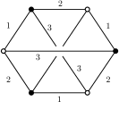
Figure 10: Some rank-six invariants with no Hermitian symmetry, respectively of order 6 (left) and 18 (right). The first one, the complete bipartite graph $K_{3,3}$, is not-melonic, but the second is melonic.

Consider in more detail the $D=3$ bubbles with six vertices, pictured on the left of Figure 10 and in Figure 11. The latest are positive and pictured along with a choice of edge-cut. They are also melonic Gurau:2011xp , which allows an easy identification of the $1/N$ expansion of the corresponding interacting models. The first one, the complete bipartite graph $K_{3,3}$, also called utility graph, is non-positive, non-melonic and non-planar, and will not be studied further in this paper.

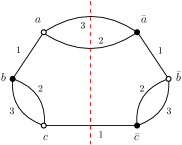
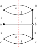
Figure 11: Melonic $D=3$ bubbles with 6 vertices

IV.3 Intermediate Field Representation

Theorem 5.

For any positive $\mathcal{B}$ with $2k(\mathcal{B})$ vertices the partition function $Z_{\mathcal{B}}(\lambda,N)$ has an HIF representation in the sense of Definition 3

$$Z_{\mathcal{B}}(\lambda,N)=\int d\nu(\xi)e^{-\operatorname{Tr}\ln\bigl{[}\mathds{1}^{\Gamma(\mathcal{B})}-g_{\mathcal{B}}\mathfrak{M}_{\mathcal{B}}(\xi)\bigr{]}},$$ (81)

in which

• the Gaussian measure $d\nu(\xi)$ is of the mixed Gaussian type in the sense of Definition 2,

• $g_{\mathcal{B}}=\lambda{\frac{1}{2k(\mathcal{B})}}N^{\frac{-s(\mathcal{B})}{2k(\mathcal{B})}}$,

• the matrix $\mathfrak{M}_{\mathcal{B}}(\xi)=i{\bf C}_{\mathcal{B}}.\mathfrak{H}_{\mathcal{B}}(\xi)$ is a $N^{\Gamma(\mathcal{B})}\times N^{\Gamma(\mathcal{B})}$ matrix, with $\Gamma(\mathcal{B})$ an integer depending on the following developments (see the end of subsection IV.3.2)

• ${\bf C}_{\mathcal{B}}$ is a mixed covariance, i.e. a direct sum of blocks of type $\mathds{1}$ (size N identity matrix) and $\begin{pmatrix}0&-i\mathds{1}_{i}\\ -i\mathds{1}_{i}&0\end{pmatrix}$ factors ($\mathds{1}_{i}$ being a size $i$ identity matrix),

• the matrix $\mathfrak{H}_{\mathcal{B}}$ is linear in the $\{\xi\}$ variables and Hermitian when these variables are taken on undeformed contours, i.e. at $\epsilon=0$.

IV.3.1 First step, along the cut

We choose an arbitrary ordering of the vertices in $F$ and name them $\{a,b,c,\cdots\}$ accordingly. As the vertices in $\bar{F}$ each have a single associated vertex in $\{a,b,c,\cdots\}$, they inherit the order and we name them $\{\bar{a},\bar{b},\bar{c},\cdots\}$, as shown in Figure 8. In this section, as in the section that deals with matrix invariants, each successive splitting will introduce new intermediate fields. The edge-cut $\mathcal{I}$ will require the introduction of a tensor field $\sigma$ of rank $\lvert\mathcal{I}\rvert$, that may have more than one index summed up e.g. with the first index of some tensor $T$ or $\bar{T}$. To distinguish between edges of the same color reaching such a vertex $\sigma$, we give new colors to the edges of the cut. An edge of color $i\in\llbracket 1,D\rrbracket$ now gets color $i_{j}$, where $j$ is the name of the tensor vertex they link. This goes back to distinguishing the corresponding copies of the Hilbert spaces ${\cal{H}}_{i_{j}}$ for different values of $j$. This is only necessary when more than one edge of the same color belongs to the cut. To an edge-cut $\mathcal{I}$ as defined above is associated the set $I$ of colors of its edges. For instance, the set $I$ corresponding to the edge-cut $\mathcal{I}$ in Figure 8 is $I=\{1_{a},1_{b},2_{d},2_{g},3,4\}$.

The tensor model associated with a positive invariant with chosen edge-cut $\mathcal{I}$ can be rewritten as

$$Z_{\mathcal{B}}(\lambda,N)=\int d\mu(T,\bar{T})e^{-\lambda N^{-s(\mathcal{B}}F(T,\bar{T})._{I}\bar{F}(T,\bar{T})},$$ (82)

where $s$ is the appropriate scaling associated to the invariant considered to ensure a non-trivial limit as $N\to\infty$ $d\mu(T,\bar{T})=\prod_{i_{1},...,i_{D}=1}^{N}dT_{i_{1},...,i_{D}}d\bar{T}_{i_{1},...,i_{D}}e^{-N^{D-1}T_{i_{1},...,i_{D}}\bar{T}_{i_{1},...,i_{D}}}$.

We generalize now the developments of the matrix section. Relations (21) and (22), which formally justify every upcoming intermediate field split, become

$$e^{-gA._{I}B}=\int d\mu^{c}(\Phi)e^{i\sqrt{g}\,(A._{I}\Phi+B._{I}\bar{\Phi})},$$ (83)

and variations for intermediate fields of imaginary covariances $\pm i$

$$e^{-gA._{I}B}=\int d\mu^{c}_{\pm i}(\Phi)e^{i\sqrt{g}\,(A._{I}\Phi\mp B._{I}\bar{\Phi})},$$ (84)

where now $A,B,\Phi$ are tensors.

Again, Gaussian imaginary integrals are considered in this section in the $\epsilon\to 0$ formal limit, and the corresponding computations will be justified by reinstating later the $\epsilon$ regulator, as in the matrix section.

As sketched above, we decompose the bubble $\mathcal{B}$ along the edge-cut $\mathcal{I}$. This requires the introduction of an intermediate tensor field $\sigma$ of rank $\lvert I\rvert$.

$$Z_{\mathcal{B}}(\lambda,N)=\int d\mu(T,\bar{T})e^{-\lambda N^{-s(\mathcal{B})}F._{I}\bar{F}}=\int d\mu(T,\bar{T})d\mu(\sigma,\bar{\sigma})e^{i\sqrt{\lambda N^{-s(\mathcal{B})}}\bigl{[}F._{I}\bar{\sigma}+\sigma._{I}\bar{F}\bigr{]}},$$ (85)

as pictured in Figure 12. The contraction of the $\kappa$’th index of $\sigma$ or $\bar{\sigma}$ with the $i$th index of some other tensor $T$ or $\bar{T}$ of the boundary of $\bar{F}$ denoted $j$ is graphically represented by an edge of color $\kappa=i_{j}\in I$. As before for matrices, the tensor $\sigma$ (resp. $\bar{\sigma}$) will be represented by a white (resp. black) square. For instance, the contraction of $\bar{\sigma}$ and the boundary of $F$ (if $T$ is of rank 4) in Figure 12 is :

$$\sum_{i_{1_{a}},i_{1_{b}},i_{2_{d}},i_{2_{g}},i_{3},i_{4}}T_{i_{1_{a}},h_{2},h_{3},h_{4}}\bar{T}_{i_{1_{b}},j_{2},j_{3},j_{4}}T_{k_{1},i_{2_{d}},k_{3},k_{4}}\bar{T}_{l_{1},i_{2_{g}},l_{3},l_{4}}T_{m_{1},m_{2},i_{3},m_{4}}T_{n_{1},n_{2},n_{3},i_{4}}\bar{\sigma}_{i_{1_{a}},i_{1_{b}},i_{2_{c}},i_{2_{e}},i_{3},i_{4}}.$$ (86)

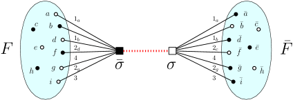
Figure 12: Intermediate field along the edge-cut $\mathcal{I}$.

The examples of the positive $D=3$ bubble with 6 vertices are shown in Figure 13.

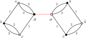
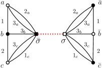
Figure 13: Positive $D=3$ bubbles with 6 vertices and intermediate field along the chosen cut.

Remark The non-crossing condition is important. When the product between $F$ and $\bar{F}$ crosses and we still implement the intermediate field decomposition, as illustrated in Figure 14 in the case of the $K_{3,3}$ graph, which is the only non-positive $D=3$ bubble with 6 vertices, we get either unitary invariants or Hermiticity but not both.

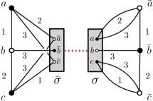
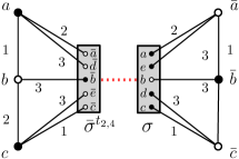
Figure 14: Non-positive $K_{3,3}$ bubble. On the left is a unitary intermediate field decomposition, which produces a non-Hermitian term. On the right is a Hermitian term which is not unitary invariant.

IV.3.2 Full decomposition

We now pair $\bar{\sigma}$ with the first tensor $a$. The contraction $F._{I}\bar{\sigma}$, which is graphically represented by a connected graph, can be rewritten in order to make this pairing explicit. We denote $\mathcal{I}_{1}$ the edge-cut which separates tensors $a$ and $\bar{\sigma}$ from the rest, $\bar{F}_{1}$, of its connected component, $\mathcal{J}_{1}$ the set of edges between tensor $a$ and $\bar{F}_{1}$, and the edges in $\tilde{\mathcal{J}}_{1}$ are the other edges reaching $a$, all contracted with $\sigma$. Note that $\mathcal{J}_{1}$ is not empty if the initial bubble has more than 2 vertices, which is the case considered here.

As before for $\mathcal{I}$, we change the colors of the edges in $\mathcal{I}_{1}$ by adding the vertex they reach in $\bar{F}_{1}$ as a subscript, and denote $I_{1}$ the corresponding set of colors. Note that if an edge in $\mathcal{I}_{1}$ of color $i\in\llbracket 1,D\rrbracket$ reaches a vertex $j\in\{a,b,\cdots\}$ which previously belonged to the boundary of $F$, then that edge already carries color $i_{j}$ from the previous splitting.

To the subset $\mathcal{J}_{1}\subset\mathcal{I}_{1}$ is associated the corresponding subset $J_{1}\subset I_{1}$. The edges in $\tilde{\mathcal{J}}_{1}$ are precisely those with color $i_{a}\in I$, where $i$ spans all the color of $\llbracket 1,D\rrbracket$ that are not in $I_{1}$. Those new sets of colors are such that $I=(I_{1}\setminus J_{1})\sqcup\tilde{J}_{1}$, and $I_{1}=J_{1}\sqcup(I\setminus\tilde{J}_{1})$, which is easily seen on Figure 15, with the convention that $\alpha_{0}=\sigma$. This allows to re-express

$$F._{I}\bar{\sigma}=[\bar{F}_{1}._{J_{1}}T]._{I}\bar{\sigma}=\bar{F}_{1}._{I_{1}}[T._{\tilde{J}_{1}}\bar{\sigma}].$$ (87)

For an initial bubble $\mathcal{B}$ with $2k(\mathcal{B})$ vertices, we define

$$g_{\mathcal{B}}=\lambda^{\frac{1}{2k(\mathcal{B})}}N^{\frac{-s(\mathcal{B})}{2k(\mathcal{B})}},$$ (88)

and generalize the trick we used in the matrix section,

$$\sqrt{\lambda N^{-s(\mathcal{B})}}\bigl{[}F._{I}\bar{\sigma}+\sigma._{I}\bar{F}\bigr{]} = g_{\mathcal{B}}^{k}\bigl{[}\bar{F}_{1}._{I_{1}}[T._{\tilde{J}_{1}}\bar{\sigma}]+[\bar{T}._{\tilde{J}_{1}}\sigma]._{I_{1}}F_{1}\bigr{]}$$ (90)

$$= \frac{1}{2}\bigl{[}(g_{\mathcal{B}}^{k-1}\bar{F}_{1}+g_{\mathcal{B}}[\bar{T}._{\tilde{J}_{1}}\sigma])._{I_{1}}(g_{\mathcal{B}}[T._{\tilde{J}_{1}}\bar{\sigma}]+g_{\mathcal{B}}^{k-1}F_{1})$$

$$\hskip 85.35826pt+(g_{\mathcal{B}}^{k-1}\bar{F}_{1}-g_{\mathcal{B}}[\bar{T}._{\tilde{J}_{1}}\sigma])._{I_{1}}(g_{\mathcal{B}}[T._{\tilde{J}_{1}}\bar{\sigma}]-g_{\mathcal{B}}^{k-1}F_{1})\bigr{]}.$$

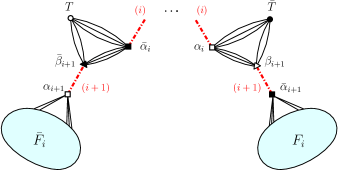
Figure 15: Step $i$ of the intermediate field decomposition, which also applies for $i=0$, in which case $\alpha_{0}=\sigma$.

Now applying (84) with complex intermediate tensor fields $a_{1}$ and $b_{1}$ of covariances $-i$ and $+i$ respectively,

$$e^{-\lambda N^{-s(\mathcal{B})}F._{I}\bar{F}} =\int d\mu^{c}(\sigma)d\mu^{c}_{\pm i}(a_{1},b_{1})e^{\frac{i}{\sqrt{2}}\bigl{[}g_{\mathcal{B}}^{k-1}\bar{F}_{1}._{I_{1}}(a_{1}+b_{1})+g_{\mathcal{B}}[T._{\tilde{J}_{1}}\bar{\sigma}]._{I_{1}}(\bar{a}_{1}-\bar{b}_{1})+c.c.\bigr{]}}$$ (91)

where the measure is $d\mu^{c}_{\pm i}(a_{1},b_{1})=d\mu^{c}_{-i}(a_{1})d\mu^{c}_{+i}(b_{1})$ and $c.c.$ stands for complex conjugate.

As in the matrix subsection, we now change variables,

$$\alpha_{1}=\frac{a_{1}+b_{1}}{\sqrt{2}},\quad\beta_{1}=\frac{a_{1}-b_{1}}{\sqrt{2}},$$ (92)

and complex conjugates. With those variables,

$$e^{-\lambda N^{-s(\mathcal{B})}F._{I}\bar{F}} =\int d\mu^{c}(\sigma)d\mu^{c}_{X}(\alpha_{1},\beta_{1})e^{i\bigl{[}g_{\mathcal{B}}^{k-1}\bar{F}_{1}._{I_{1}}\alpha_{1}+g_{\mathcal{B}}[T._{\tilde{J}_{1}}\bar{\sigma}]._{I_{1}}\bar{\beta}_{1}+c.c.\bigr{]}},$$ (93)

the Gaussian measure $d\mu^{c}_{X}$ being defined by its moments, that all vanish apart from

$$\forall i_{1},\cdots,i_{\lvert I_{1}\rvert}\in\{1,...,N\},\quad<\alpha_{1\mid i_{1},\cdots,i_{\lvert I_{1}\rvert}}\bar{\beta}_{1\mid i_{1},\cdots,i_{\lvert I_{1}\rvert}}>_{X}=<\bar{\alpha}_{1\mid i_{1},\cdots,i_{\lvert I_{1}\rvert}}\beta_{1\mid i_{1},\cdots,i_{\lvert I_{1}\rvert}}>_{X}=-i.$$ (94)

The term $\bar{F}_{1}._{I_{1}}\alpha_{1}$ is of the exact same form as the term $\bar{F}._{I}\sigma$ before. We apply therefore the same reasoning again. We couple $\alpha_{1}$ with the first black vertex $a^{\prime}$ in the boundary of $\bar{F}_{1}$ such that there existed an edge $(aa^{\prime})\in\mathcal{J}_{1}$ in the previous step. It is always possible as $\mathcal{J}_{1}$ is not empty. We denote $\mathcal{I}_{2}$ the edge-cut which separates tensors $a^{\prime}$ and $\alpha_{1}$ from the rest, $F_{2}$, of its connected component, $\mathcal{J}_{2}$ the set of edges between tensor $a^{\prime}$ and $F_{2}$, $\tilde{\mathcal{J}}_{1}$ those between $a^{\prime}$ and $\alpha_{1}$, and as before we change the colors of the edges when necessary and name $I_{2}$, $J_{2}$, $\tilde{J}_{2}$ the associated sets of colors. Our choice for vertex $a^{\prime}$ ensures that $\tilde{J}_{2}\cap J_{1}\neq\emptyset$. As in the previous step, $\bar{F}_{1}._{I_{1}}\alpha_{1}=[F_{2}._{J_{2}}\bar{T}]._{I_{1}}\alpha_{1}=F_{2}._{I_{2}}[\bar{T}._{\tilde{J}_{2}}\alpha_{1}]$, and after developments such as in (90)-(94),

$$e^{ig_{\mathcal{B}}^{k-1}\bar{F}_{1}._{I_{1}}\alpha_{1}}=\int d\mu^{c}_{X}(\alpha_{2},\beta_{2})e^{i\bigl{[}g_{\mathcal{B}}^{k-2}F_{2}._{I_{2}}\bar{\alpha}_{2}+g_{\mathcal{B}}[\bar{T}._{\tilde{J}_{2}}\alpha_{1}]._{I_{2}}\beta_{2}+c.c.\bigr{]}}.$$ (95)

Note that we could choose any black vertex in $\bar{F}_{1}$ but this choice ensures that $\tilde{J}_{2}$ is not empty. We also stress that we use pairings which are not necessarily optimal, in the sense that we do noty try to introduce intermediate fields of the smallest possible ranks.

We inductively apply the same reasoning until step $k-2$, which leaves us with $F_{k-1}$ having only two remaining tensor vertices. As we decomposed the initial interaction into a sum of connected interactions involving only three tensors each, we shall later be able to do a Gaussian integration over $T$ and other fields. The partition function currently has the following expression

$$Z_{\mathcal{B}}(\lambda,N) = \int d\mu^{c}(T)d\mu^{c}(\sigma)\prod_{j=1}^{k-2}d\mu^{c}_{X}(\alpha_{j},\beta_{j})e^{ig_{\mathcal{B}}\bigl{(}[\bar{T}._{\tilde{J}_{1}}\sigma]._{I_{1}}\beta_{1}\,+\,[\bar{T}._{\tilde{J}_{2}}\alpha_{1}]._{I_{2}}\beta_{2}\,+\,[\bar{T}._{\tilde{J}_{k-2}}\alpha_{k-3}]._{I_{k-2}}\beta_{k-2}\,+\cdots}\hskip 56.9055pt$$

$$\hskip 284.52756pt{}^{\cdots+\,g_{\mathcal{B}}[\bar{T}._{J_{k-1}}T]._{I_{k-2}}\alpha_{k-2}\,+c.c.\bigr{)}},$$

where we recall that $k$ is the number of vertices of $F$ and $c.c.$ stands for complex conjugate. The $i$’th splitting introduces the tensor intermediate fields $\alpha_{i+1}$ and $\beta_{i+1}$, with complex covariances as in (94) and is represented in Figure 15 (this may also apply for $\alpha_{0}=\sigma$). As in the two first steps, the sets of newly introduced colors are such that $J_{i}$ is non-empty, and

$$\tilde{J}_{i+1}\cap J_{i}\neq\emptyset,\quad\textrm{and}\quad I_{i+1}\setminus J_{i+1}=I_{i}\setminus\tilde{J}_{i+1},$$ (97)

and in particular,

$$I_{i}=(I_{i+1}\setminus J_{i+1})\sqcup\tilde{J}_{i+1}=J_{i}\sqcup(I_{i-1}\setminus\tilde{J}_{i}),$$ (98)

the sets having empty intersections because two edges of the same color cannot reach the same tensor.

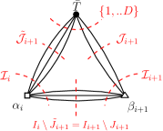
Figure 16: Triangular connected term in the full decomposition (IV.3.2).

As each connected interaction is now a contraction of three tensors, $\bar{T}$, $\alpha_{i}$, and $\beta_{i}$ (or complex conjugates), we may now naturally organize each tensor $\alpha_{i}$ (resp. $\beta_{i}$) as a rectangular matrix of size $N^{\lvert\tilde{J}_{i+1}\rvert}\times N^{\lvert I_{i}\setminus\tilde{J}_{i+1}\rvert}$ (resp. $N^{\lvert J_{i}\rvert}\times N^{\lvert I_{i}\setminus J_{i}\rvert}$), in the sense that we specify its first and second sets of indices, respectively those contracted to $T$ and the remaining ones (see Figure 16). More precisely, we understand $\alpha_{i}$ and $\beta_{i}$ as matrices of linear maps :

$$\begin{array}[]{rll}\otimes_{j\in{I_{i}\setminus\tilde{J}_{i+1}}}{\cal{H}}_{j}&\longrightarrow&\otimes_{j\in\tilde{J}_{i+1}}{\cal{H}}_{j}\\ \\ X_{I_{i}\setminus\tilde{J}_{i+1}}&\longrightarrow&\sum_{I_{i}\setminus\tilde{J}_{i+1}}\alpha_{i\ \mid\ \tilde{J}_{i+1}\ ;\ I_{i}\setminus\tilde{J}_{i+1}}\ X_{I_{i}\setminus\tilde{J}_{i+1}}\end{array}\ \textrm{and}\qquad\begin{array}[]{rll}\otimes_{j\in{I_{i}\setminus J_{i}}}{\cal{H}}_{j}&\longrightarrow&\otimes_{j\in J_{i}}{\cal{H}}_{j}\\ \\ X_{I_{i}\setminus J_{i}}&\longrightarrow&\sum_{I_{i}\setminus J_{i}}\beta_{i\ \mid\ J_{i}\ ;\ I_{i}\setminus J_{i}}\ X_{I_{i}\setminus J_{i}}.\end{array}$$

For the last term, $[\bar{T}._{J_{k-1}}T]._{I_{k-2}}\alpha_{k-2}$, the convention is that $\alpha_{k-2}$ is a $N^{\lvert J_{k-1}\rvert}\times N^{\lvert\tilde{J}_{k-1}\rvert}$ square matrix, since $\lvert J_{k-1}\rvert=\lvert\tilde{J}_{k-1}\rvert=D-\lvert J_{k-1}\rvert$. These conventions will be very useful at the end of the section. The sizes of the matrices are easily readable on the connected triangular graphs of the graphical representation of the full intermediate field decomposition (Figure 16 and examples in subsection IV.5). The following relations are also verified:

$$\bar{F}_{i}._{I_{i}}\alpha_{i}\ =\ [\bar{T}._{J_{i+1}}F_{i+1}]._{I_{i}}\alpha_{i}\ =\ [\bar{T}._{\tilde{J}_{i+1}}\alpha_{i}]._{I_{i+1}}F_{i+1},$$ (99)

and similarly after the intermediate field split (Figure 16),

$$[\bar{T}._{J_{i+1}}\beta_{i+1}]._{I_{i}}\alpha_{i}\ =\ [\bar{T}._{\tilde{J}_{i+1}}\alpha_{i}]._{I_{i+1}}\beta_{i+1}\ =\ \bar{T}._{\llbracket 1,D\rrbracket}\ [\beta_{i+1}\,\alpha_{i}^{\mathrm{T}}],$$ (100)

where with our new convention, $\beta_{i+1}\alpha_{i}^{\mathrm{T}}\$ is a $N^{\lvert J_{i+1}\rvert}\times N^{\lvert\tilde{J}_{i+1}\rvert}$ matrix.

We shall now integrate over a subset of the intermediate fields using the following relation,

$$\int d\mu^{c}_{X}(\alpha,\beta)e^{i(A._{I}\alpha+B._{I}\beta+C._{I}\bar{\alpha}+D._{I}\bar{\beta})}=e^{i(A._{I}D+B._{I}C)}.$$ (101)

The integration is performed over $T$ and all $\alpha_{k-1-2j}$, $\beta_{k-1-2j}$, for $j\in\{1,...,\lfloor\frac{k}{2}\rfloor\}$, i.e.

• for $k$ odd, over the $k$ intermediate tensor fields $T$, $\sigma$, all even $\alpha_{2j}$, $\beta_{2j}$, for $j\in\{1,..,\frac{k-3}{2}\}$ and complex conjugates.

• for $k$ even, over the $k$ intermediate tensor fields $T$, all odd $\alpha_{2j-1}$, $\beta_{2j-1}$, for $j\in\{1,..,\frac{k-2}{2}\}$ and complex conjugates.

To use (101) we must rewrite, using relation (100),

$$[\bar{T}._{\tilde{J}_{k-2j}}\alpha_{k-2j-1}]._{I_{k-2j}}\beta_{k-2j}=[\bar{T}._{J_{k-2j}}\beta_{k-2j}]._{I_{k-2j-1}}\alpha_{k-2j-1}.$$ (102)

Each integration step is then done independently of the others:

$$\int d\mu^{c}_{X}(\alpha_{k-1-2j},\beta_{k-1-2j})e^{ig_{\mathcal{B}}\bigl{(}[\bar{T}._{J_{k-2j}}\beta_{k-2j}]._{I_{k-2j-1}}\alpha_{k-2j-1}+[\bar{T}._{\tilde{J}_{k-2j-1}}\alpha_{k-2(j+1)}]._{I_{k-2j-1}}\beta_{k-2j-1}+c.c.\bigr{)}}$$

$$=\ e^{ig_{\mathcal{B}}^{2}\bigl{(}[\bar{T}._{J_{k-2j}}\beta_{k-2j}]._{I_{k-2j-1}}[T._{\tilde{J}_{k-2j-1}}\bar{\alpha}_{k-2(j+1)}]+c.c.\bigr{)}},\$$ (103)

except for the $\sigma$ integration for $k$ odd,

$$\int d\mu^{c}(\sigma)e^{ig_{\mathcal{B}}\bigl{(}[\beta_{1}._{J_{1}}\bar{T}]._{I}\sigma+c.c.\bigr{)}}=\ e^{-g_{\mathcal{B}}^{2}\bigl{(}[\bar{T}._{J_{1}}\beta_{1}]._{I}[\bar{\beta}_{1}._{J_{1}}T]\bigr{)}},\$$ (104)

which leaves us with the integration of the $T$ variable in

$$Z_{\mathcal{B}}(\lambda,N)=\int d\nu(\xi)d\mu^{c}(T)e^{ig_{\mathcal{B}}^{2}\biggl{(}\sum_{j=1}^{\lfloor\frac{k}{2}\rfloor}[\bar{T}._{J_{k-2j}}\beta_{k-2j}]._{I_{k-2j-1}}[T._{\tilde{J}_{k-2j-1}}\bar{\alpha}_{k-2(j+1)}]}$$

$${}^{+\,[\bar{T}._{J_{k-1}}T]._{I_{k-2}}\bar{\alpha}_{k-2}\,+\,c.c.\,+\,i\eta(k)[\bar{T}._{J_{1}}\beta_{1}]._{I}[\bar{\beta}_{1}._{J_{1}}T]\biggr{)}},$$

in which $\xi=(...\alpha_{k-2j},\beta_{k-2j},...)$ is the vector containing the $k-1$ remaining variables, $\xi_{odd}=(\alpha_{1},\beta_{1},...,\alpha_{k-2},\beta_{k-2})$ and $\xi_{even}=(\sigma,\alpha_{2},\beta_{2},...,\alpha_{k-2},\beta_{k-2})$, and $\alpha_{0}=\sigma$, $\beta_{k}=1$, $\alpha_{<0}=0$ and $\beta_{\leq 0}=0$, and $\eta(k)$ is 0 for $k$ even and 1 for $k$ odd.

In order to perform the integration over $T$, we must factorize

$$[\bar{T}._{J_{k-1}}T]._{I_{k-2}}\bar{\alpha}_{k-2} = \sum_{J_{k-1},\tilde{J}_{k-1},J^{\prime}_{k-1},\tilde{J}^{\prime}_{k-1}}\bar{T}_{J_{k-1}\,;\,\tilde{J}_{k-1}}\mathds{1}_{J_{k-1}\,;\,J^{\prime}_{k-1}}\alpha_{k-2\mid\tilde{J}_{k-1}\,;\,\tilde{J}^{\prime}_{k-1}}T_{J^{\prime}_{k-1}\,;\,\tilde{J}^{\prime}_{k-1}}$$ (106)

$$= \ \ \bar{T}._{\llbracket 1,D\rrbracket}\bigl{(}\ \alpha_{k-2}\otimes\mathds{1}^{\otimes\lvert J_{k-1}\rvert}\bigr{)}._{\llbracket 1,D\rrbracket}T,$$

since the indices that aren’t contracted in $[\bar{T}._{J_{k-1}}T]$ are both the indices of $\bar{T}$ and of $T$ with colors in $\tilde{J}_{k-1}$. Also tensor $T$ does not see the subscript colors, and regardless of those, $J_{k-1}\sqcup\tilde{J}_{k-1}=\llbracket 1,D\rrbracket$. In these equations, $\alpha_{k-2}$ is to be understood as a square $N^{\lvert\tilde{J}_{k-1}\rvert}\times N^{\lvert\tilde{J}_{k-1}\rvert}$ matrix, as outlined before.

Similarly, as $I=(I_{1}\setminus J_{1})\sqcup\tilde{J}_{1}$, the indices of $\beta_{1}$ in $[\bar{T}._{J_{1}}\beta_{1}]._{I}[\bar{\beta}_{1}._{J_{1}}T]$ that are not contracted with $\bar{T}$ are precisely the indices in $I$ that are summed up with those of the same colors in $\bar{\beta}_{1}$, so that

$$[\bar{T}._{J_{1}}\beta_{1}]._{I}[\bar{\beta}_{1}._{J_{1}}T] = \sum_{J_{1},\tilde{J}_{1},J^{\prime}_{1},\tilde{J}^{\prime}_{1}}\bar{T}_{J_{1}\,;\,\tilde{J}_{1}}[\beta_{1}._{I_{1}\setminus J_{1}}\bar{\beta}_{1}]_{J_{1}\,;\,J^{\prime}_{1}}\mathds{1}_{\tilde{J}_{1}\,;\,\tilde{J}^{\prime}_{1}}T_{J^{\prime}_{1}\,;\,\tilde{J}^{\prime}_{1}}$$ (107)

$$= \ \ \bar{T}._{\llbracket 1,D\rrbracket}\bigl{(}\ \beta_{1}\beta_{1}^{\dagger}\otimes\mathds{1}^{\otimes\lvert\tilde{J}_{1}\rvert}\bigr{)}._{\llbracket 1,D\rrbracket}T,$$

in which $\beta_{1}\beta_{1}^{\dagger}$ is a square $N^{\lvert J_{1}\rvert}\times N^{\lvert J_{1}\rvert}$ matrix.

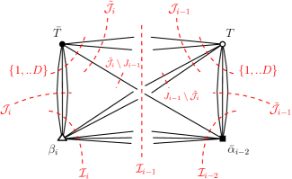
Figure 17: Terms in $\mathbf{H_{k}}$ after integration, taking $i=k-2j$.

The other terms of the sum require a slightly subtler treatment, as $J_{k-2j}$ and $\tilde{J}_{k-2j-1}$ may have a non-empty intersection (see Figure 17),

$$[\bar{T}._{J_{i}}\beta_{i}]._{I_{i-1}}[T._{\tilde{J}_{i-1}}\bar{\alpha}_{i-2}] = \sum_{\begin{subarray}{c}{J_{i},\ \tilde{J}_{i}\cap J_{i-1},\ \tilde{J}_{i-1},\ \ }\\ {\tilde{J}_{i}\setminus J_{i-1},\ J_{i-1}\setminus\tilde{J}_{i}}\end{subarray}}$$ (108)

$$\bar{T}_{J_{i}\,;\,\tilde{J}_{i}\setminus J_{i-1}\,;\,\tilde{J}_{i}\cap J_{i-1}}[\beta_{i}._{I_{i-1}\setminus(J_{i-1}\cup\tilde{J}_{i})}\bar{\alpha}_{i-2}]_{J_{i}\,;\,\tilde{J}_{i}\setminus J_{i-1}|\tilde{J}_{i-1}\,;\,J_{i-1}\setminus\tilde{J}_{i}}T_{\tilde{J}_{i-1}\,;\,J_{i-1}\setminus\tilde{J}_{i}\,;\ \tilde{J}_{i}\cap J_{i-1}}$$

$$= \ \ \bar{T}._{\llbracket 1,D\rrbracket}\biggl{(}[\beta_{i}._{I_{i-1}\setminus(J_{i-1}\cup\tilde{J}_{i})}\bar{\alpha}_{i-2}]\otimes\mathds{1}^{\otimes\lvert\tilde{J}_{i}\cap J_{i-1}\rvert}\biggr{)}._{\llbracket 1,D\rrbracket}T,$$

where $[\beta_{i}._{I_{i-1}\setminus(J_{i-1}\cup\tilde{J}_{i})}\bar{\alpha}_{i-2}]$ might be understood as a $N^{D-\lvert\tilde{J}_{i}\cap J_{i-1}\rvert}\times N^{D-\lvert\tilde{J}_{i}\cap J_{i-1}\rvert}$ square matrix with its first half indices contracted to sub-indices of $\bar{T}$ and the other half to sub-indices of $T$, since $J_{i}\sqcup\tilde{J}_{i}\setminus J_{i-1}$ corresponds to the edges reaching $\bar{T}$ that are not in $\tilde{J}_{i}\cap J_{i-1}$, and $\tilde{J}_{i-1}\sqcup J_{i-1}\setminus\tilde{J}_{i}$ to the edges reaching $T$ that are not in $\tilde{J}_{i}\cap J_{i-1}$ (Figure 17). This might be rewritten using the matrix conventions introduced earlier,

$$[\bar{T}._{J_{i}}\beta_{i}]._{I_{i-1}}[T._{\tilde{J}_{i-1}}\bar{\alpha}_{i-2}]=\ \bar{T}._{\llbracket 1,D\rrbracket}\biggl{(}\ [\beta_{i}\otimes\mathds{1}^{\lvert\tilde{J}_{i}\rvert}].[\alpha_{i-2}^{\dagger}\otimes\mathds{1}^{\otimes\lvert J_{i-1}\rvert}]\ \biggr{)}._{\llbracket 1,D\rrbracket}T,$$ (109)

where the tensorial products might be understood as a Kronecker product of matrices. The central dot in (109) stands for the usual matrix product. Recall indeed that $\beta_{i}\otimes\mathds{1}^{\lvert\tilde{J}_{i}\rvert}:\otimes_{j\in(I_{i-1}\setminus\tilde{J}_{i})\sqcup\tilde{J}_{i}}{\cal{H}}_{j}\longrightarrow\otimes_{j\in J_{i}\sqcup\tilde{J}_{i}}{\cal{H}}_{j}$, and $\alpha_{i-2}^{\dagger}\otimes\mathds{1}^{\otimes\lvert J_{i-1}\rvert}:\otimes_{j\in\tilde{J}_{i-1}\sqcup J_{i-1}}{\cal{H}}_{j}\longrightarrow\otimes_{j\in(I_{i-1}\setminus J_{i-1})\sqcup J_{i-1}}{\cal{H}}_{j}$.

The complex conjugate term gives

$$[\bar{T}._{\tilde{J}_{i-1}}\alpha_{i-2}]._{I_{i-1}}[T._{J_{i}}\bar{\beta}_{i}] = \bar{T}._{\llbracket 1,D\rrbracket}\biggl{(}[\alpha_{i-2}._{I_{i-1}\setminus(J_{i-1}\cup\tilde{J}_{i})}\bar{\beta}_{i}]\otimes\mathds{1}^{\otimes\lvert\tilde{J}_{i}\cap J_{i-1}\rvert}\biggr{)}._{\llbracket 1,D\rrbracket}T$$ (110)

$$= \bar{T}._{\llbracket 1,D\rrbracket}\biggl{(}[\beta_{i}._{I_{i-1}\setminus(J_{i-1}\cup\tilde{J}_{i})}\bar{\alpha}_{i-2}]\otimes\mathds{1}^{\otimes\lvert\tilde{J}_{i}\cap J_{i-1}\rvert}\biggr{)}^{\dagger}._{\llbracket 1,D\rrbracket}T$$

$$= \ \bar{T}._{\llbracket 1,D\rrbracket}\biggl{(}\ [\alpha_{i-2}\otimes\mathds{1}^{\otimes\lvert J_{i-1}\rvert}].[\beta_{i}^{\dagger}\otimes\mathds{1}^{\lvert\tilde{J}_{i}\rvert}]\ \biggr{)}._{\llbracket 1,D\rrbracket}T,$$

and the $\beta_{1}$ term may also be written as

$$[\bar{T}._{J_{1}}\beta_{1}]._{I}[\bar{\beta}_{1}._{J_{1}}T]=\ \bar{T}._{\llbracket 1,D\rrbracket}\biggl{(}\ [\beta_{1}\otimes\mathds{1}^{\lvert\tilde{J}_{1}\rvert}].[\beta_{1}\otimes\mathds{1}^{\lvert\tilde{J}_{1}\rvert}]^{\dagger}\ \biggr{)}._{\llbracket 1,D\rrbracket}T.$$ (111)

so that if we denote the $N^{D}\times N^{D}$ Hermitian matrix

$$\mathbf{H}_{\mathcal{B}}(\xi) = \sum_{j=0}^{\lfloor\frac{k}{2}\rfloor}\ \ [\beta_{k-2j}._{I_{k-2j-1}\setminus(J_{k-2j-1}\cup\tilde{J}_{k-2j})}\bar{\alpha}_{k-2(j+1)}]\otimes\mathds{1}^{\otimes\lvert\tilde{J}_{k-2j}\cap J_{k-2j-1}\rvert}+c.t.$$ (112)

$$= \sum_{j=0}^{\lfloor\frac{k}{2}\rfloor}\ \ [\alpha_{i-2}\otimes\mathds{1}^{\otimes\lvert J_{i-1}\rvert}].[\beta_{i}^{\dagger}\otimes\mathds{1}^{\lvert\tilde{J}_{i}\rvert}]+c.t.,$$

the integration over $T$ leads to the following expression of the partition function,

$$Z_{\mathcal{B}}(\lambda,N)=\int d\nu(\xi)e^{-\operatorname{Tr}\ln\bigl{[}\,\mathds{1}^{\otimes D}-\,g_{\mathcal{B}}^{2}\bigl{(}\,i\mathbf{H}_{\mathcal{B}}(\xi)\ -\ \eta(k)\beta_{1}\beta_{1}^{\dagger}\otimes\mathds{1}^{\otimes\lvert\tilde{J}_{1}\rvert}\,\bigr{)}\ \bigr{]}},$$ (113)

where $d\nu$ factorizes over the measures $d\mu_{o}^{c}$ of each $\alpha,\beta$ pair plus the measure $d\mu^{c}(\sigma)$ for $k$ even, and $\eta(k)$ is 0 for $k$ even and 1 for $k$ odd.

In the previous expression however, it may be possible to factorize some identity factors of the sum of tensorial products when they act on the same color $i$. Here, only the color as defined in the first place matters, i.e. identity factors acting on spaces ${\cal{H}}_{i_{a}}$ and ${\cal{H}}_{i_{b}}$ for the same $i$ are factorized. We denote $\Theta_{\mathcal{B},\{\mathcal{I}_{i}\}}$ the number of tensorial products of the $N\times N$ identity one can factorize in the sum $\ i\mathbf{H}_{\mathcal{B}}(\xi)\ -\ \eta(k)\beta_{1}\beta_{1}^{\dagger}\otimes\mathds{1}^{\otimes\lvert\tilde{J}_{1}\rvert}\,$. In the matrix case this $\Theta_{\mathcal{B},\{\mathcal{I}_{i}\}}$ was always exactly 1, leading to the factor $N$ in front of the logarithm in (36). In the tensor case we always choose to pair tensor $\alpha_{i}$ with a vertex of the boundary of the edge-cut $\mathcal{I}_{i}$ which belonged to $\mathcal{J}_{i}$, and we know that $\forall i,\lvert\tilde{J}_{i}\cap J_{i-1}\rvert\geq 1$ and $\lvert\tilde{J}_{1}\rvert\geq 1$, so that $\Theta_{\mathcal{B},\{\mathcal{I}_{i}\}}\geq 1$. As $\det(\mathds{1}^{\otimes\Theta}\otimes M)=\det(M)^{N^{\Theta}}$, this factorisation lays out a global factor $N^{\Theta_{\mathcal{B},\{\mathcal{I}_{i}\}}}$,

$$Z_{\mathcal{B}}(\lambda,N)=\int d\nu(\xi)e^{-N^{\Theta_{\mathcal{B},\{\mathcal{I}_{i}\}}}\operatorname{Tr}\ln\biggl{[}\,\mathds{1}^{\otimes\bigl{(}D-\Theta_{\mathcal{B},\{\mathcal{I}_{i}\}}\bigr{)}}-\,g_{\mathcal{B}}^{2}\biggl{(}\,iH_{\mathcal{B}}(\xi)\ -\ \eta(k)\beta_{1}\beta_{1}^{\dagger}\otimes\mathds{1}^{\otimes\bigl{(}\lvert\tilde{J}_{1}\rvert-\Theta_{\mathcal{B},\{\mathcal{I}_{i}\}}\bigr{)}}\,\biggr{)}\ \biggr{]}},$$ (114)

where we denoted $H_{\mathcal{B}}$ the Hermitian $N^{D-\Theta_{\mathcal{B},\{\mathcal{I}_{i}\}}}\times N^{D-\Theta_{\mathcal{B},\{\mathcal{I}_{i}\}}}$ matrix that verifies $H_{\mathcal{B}}\otimes\mathds{1}^{\otimes(\Theta_{\mathcal{B},\{\mathcal{I}_{i}\}})}=\mathbf{H}_{\mathcal{B}}$. It is straightforward to determine $\Theta$ graphically. The fields that are not integrated and thus remain in the final representation have the parity of $k$. In the graphical decomposition of the interaction into connected graphs with three vertices, among which a single $T$ or $\bar{T}$, the identity tensor products are the edges between $T$ (or $\bar{T}$) and the field which is to be integrated. $\Theta$ is the number of colors for which such an edge exists in every connected graph of order 3. See the example in subsection IV.5.

Obviously, $\Theta_{\mathcal{B},\{\mathcal{I}_{i}\}}$ depends heavily on the successive choices of edge-cuts $\mathcal{I}_{i}$. Some splittings will give a maximal value $\Theta_{\mathcal{B}}=\max_{\{\mathcal{I}_{i}\}}\Theta_{\mathcal{B},\{\mathcal{I}_{i}\}}$. We shall treat in detail the melonic examples of order 6 in $D=3$ for which we give this maximal value. From now on we write simply $\Theta$ for $\Theta_{\mathcal{B},\{\mathcal{I}_{i}\}}$.

Linear Hermitian Intermediate Field Representation

With a similar proof, Lemma 2 generalizes to rectangular matrices, so that expression (113) can be reformulated using a $N^{\Gamma(\mathcal{B})}\times N^{\Gamma(\mathcal{B})}$ determinant. $\Gamma$ is an integer that depends on the choices of edge cuts $\{I_{j}\}$, $\Gamma=3D+\lvert I\rvert+2(\lvert I_{2}\rvert+\lvert I_{4}\rvert+\cdots\lvert I_{k-3}\rvert)$ for $k$ odd, and $\Gamma=3D+2(\lvert I_{1}\rvert+\lvert I_{3}\rvert+\cdots\lvert I_{k-3}\rvert)$ for $k$ even

$$Z_{\mathcal{B}}(\lambda,N)=\int d\nu(\xi)e^{-\operatorname{Tr}\ln\bigl{[}\mathds{1}^{\otimes\Gamma(\mathcal{B})}-g_{\mathcal{B}}\mathfrak{M}_{\mathcal{B}}(\xi)\bigr{]}},$$ (115)

where $\mathfrak{M}_{\mathcal{B}}(\xi)=i{\bf C}_{\mathcal{B}}.\mathfrak{H}_{\mathcal{B}}(\xi)$, ${\bf C}_{\mathcal{B}}$ is the complex square symmetric covariance of size $N^{\Gamma(\mathcal{B})}\times N^{\Gamma(\mathcal{B})}$of the integrated fields

$${\bf C}_{odd}=\left(\begin{array}[]{ccccccc}{\mathds{1}}^{\otimes D}&\lx@intercol\hfil 0\hfil\lx@intercol\vrule\lx@intercol&&&&&\\ 0&\lx@intercol\hfil{\mathds{1}}^{\otimes\lvert I\rvert}\hfil\lx@intercol\vrule\lx@intercol&&&&&\\ \cline{1-4}\cr&\lx@intercol\hfil\hfil\lx@intercol\vrule\lx@intercol&0&\lx@intercol\hfil-i{\mathds{1}}^{\otimes\lvert I_{2}\rvert}\hfil\lx@intercol\vrule\lx@intercol&&\Large\mbox{{$0$}}&\\ &\lx@intercol\hfil\hfil\lx@intercol\vrule\lx@intercol&-i{\mathds{1}}^{\otimes\lvert I_{2}\rvert}&\lx@intercol\hfil 0\hfil\lx@intercol\vrule\lx@intercol&&&\\ \cline{3-6}\cr&&&\lx@intercol\hfil\hfil\lx@intercol\vrule\lx@intercol&0&\lx@intercol\hfil-i{\mathds{1}}^{\otimes\lvert I_{4}\rvert}\hfil\lx@intercol\vrule\lx@intercol&\\ &&\Large\mbox{{$0$}}&\lx@intercol\hfil\hfil\lx@intercol\vrule\lx@intercol&-i{\mathds{1}}^{\otimes\lvert I_{4}\rvert}&\lx@intercol\hfil 0\hfil\lx@intercol\vrule\lx@intercol&\\ \cline{5-6}\cr&&&&&&\ddots\end{array}\right),$$ (123)

$${\bf C}_{even}=\left(\begin{array}[]{cccccc}\lx@intercol\hfil{\mathds{1}}^{\otimes D}\hfil\lx@intercol\vrule\lx@intercol&&&&&\\ \cline{1-3}\cr\lx@intercol\hfil\hfil\lx@intercol\vrule\lx@intercol&0&\lx@intercol\hfil-i{\mathds{1}}^{\otimes\lvert I_{1}\rvert}\hfil\lx@intercol\vrule\lx@intercol&&\Large\mbox{{$0$}}&\\ \lx@intercol\hfil\hfil\lx@intercol\vrule\lx@intercol&-i{\mathds{1}}^{\otimes\lvert I_{1}\rvert}&\lx@intercol\hfil 0\hfil\lx@intercol\vrule\lx@intercol&&&\\ \cline{2-5}\cr&&\lx@intercol\hfil\hfil\lx@intercol\vrule\lx@intercol&0&\lx@intercol\hfil-i{\mathds{1}}^{\otimes\lvert I_{3}\rvert}\hfil\lx@intercol\vrule\lx@intercol&\\ &\Large\mbox{{$0$}}&\lx@intercol\hfil\hfil\lx@intercol\vrule\lx@intercol&-i{\mathds{1}}^{\otimes\lvert I_{3}\rvert}&\lx@intercol\hfil 0\hfil\lx@intercol\vrule\lx@intercol&\\ \cline{4-5}\cr&&&&&\ddots\end{array}\right).$$ (130)

The matrix $\mathfrak{H}_{\mathcal{B}}$ is Hermitian, and has two different forms for $k$ odd or even

$$\mathfrak{H}^{odd}_{\mathcal{B}}=\left(\begin{array}[]{c|ccccc}0&\beta_{1}\otimes\mathds{1}^{\otimes\lvert\tilde{J}_{1}\rvert}&\alpha_{1}\otimes\mathds{1}^{\otimes\lvert J_{2}\rvert}&\cdots&\alpha_{k-2}\otimes\mathds{1}^{\otimes\lvert J_{k-1}\rvert}&{\mathds{1}}^{\otimes D}\\ \hline\cr\raisebox{-4.0pt}{ $\beta_{1}^{\dagger}\otimes\mathds{1}^{\otimes\lvert\tilde{J}_{1}\rvert}$ }&&&\raisebox{-30.0pt}{{\huge\mbox{{$0$}}}}\\[-12.91663pt] \alpha_{1}^{\dagger}\otimes\mathds{1}^{\otimes\lvert J_{2}\rvert}&\\ \vdots&\\[2.15277pt] \alpha_{k-2}^{\dagger}\otimes\mathds{1}^{\otimes\lvert J_{k-1}\rvert}&\\[4.30554pt] {\mathds{1}}^{\otimes D}&\\[4.30554pt] \end{array}\right),$$ (132)

$$\mathfrak{H}^{even}_{\mathcal{B}}=\left(\begin{array}[]{c|ccccc}0&\sigma\otimes\mathds{1}^{\otimes\lvert J_{1}\rvert}&\beta_{2}\otimes\mathds{1}^{\otimes\lvert\tilde{J}_{2}\rvert}&\cdots&\alpha_{k-2}\otimes\mathds{1}^{\otimes\lvert J_{k-1}\rvert}&{\mathds{1}}^{\otimes D}\\ \hline\cr\raisebox{-4.0pt}{ $\sigma^{\dagger}\otimes\mathds{1}^{\otimes\lvert J_{1}\rvert}$}&&&\raisebox{-30.0pt}{{\huge\mbox{{$0$}}}}\\[-12.91663pt] \beta_{2}^{\dagger}\otimes\mathds{1}^{\otimes\lvert\tilde{J}_{2}\rvert}&\\ \vdots&\\[2.15277pt] \alpha_{k-2}^{\dagger}\otimes\mathds{1}^{\otimes\lvert J_{k-1}\rvert}&\\[4.30554pt] {\mathds{1}}^{\otimes D}&\\[4.30554pt] \end{array}\right).$$ (133)

In this block matrix, the various blocks may not have the same size. The $(k+1)$ blocks of the first raw are $N^{D}\times N^{\lvert I_{j}\rvert}$ rectangular matrices, where $j=i-1$ when it regards $\beta_{i}$ and $j=i+1$ when it comes to $\alpha_{i}$, which are Kronecker products

$$[\alpha_{i}\otimes\mathds{1}^{\otimes\lvert J_{i+1}\rvert}]_{m_{1},\cdots,m_{D}\ ;\ n_{1}\cdots,n_{\lvert I_{i+1}\rvert}}=[\alpha_{i}]_{m_{i_{1}},\cdots\ m_{i_{\lvert\tilde{J}_{i+1}\rvert}}\ ;\ n_{j_{1}}\cdots n_{j_{\lvert I_{i+1}\setminus J_{i+1}\rvert}}}\delta_{m_{i^{\prime}_{1}},n_{j^{\prime}_{1}}}\cdots\delta_{m_{i^{\prime}_{\lvert J_{i+1}\rvert}},n_{j^{\prime}_{\lvert J_{i+1}\rvert}}},$$ (134)

$$[\beta_{i}\otimes\mathds{1}^{\otimes\lvert\tilde{J}_{i}\rvert}]_{m_{1},\cdots,m_{D}\ ;\ n_{1}\cdots,n_{\lvert I_{i-1}\rvert}}=[\beta_{i}]_{m_{i_{1}},\cdots m_{i_{\lvert J_{i}\rvert}}\ ;\ n_{j_{1}}\cdots n_{j_{\lvert I_{i-1}\setminus\tilde{J}_{i}\rvert}}}\delta_{m_{i^{\prime}_{1}},n_{j^{\prime}_{1}}}\cdots\delta_{m_{i^{\prime}_{\lvert\tilde{J}_{i}\rvert}},n_{j^{\prime}_{\lvert\tilde{J}_{i}\rvert}}}.$$ (135)

or using the simplified notations introduced previously,

$$[\alpha_{i}\otimes\mathds{1}^{\otimes\lvert J_{i+1}\rvert}]_{J_{i+1}\sqcup\tilde{J}_{i+1}\ ;\ I_{i+1}}=\alpha_{i\ \mid\ \tilde{J}_{i+1}\ ;\ I_{i+1}\setminus J_{i+1}}\ \delta_{J_{i+1}\ ;\ J_{i+1}},$$ (136)

$$[\beta_{i}\otimes\mathds{1}^{\otimes\lvert\tilde{J}_{i}\rvert}]_{J_{i}\sqcup\tilde{J}_{i}\ ;\ I_{i-1}}=[\beta_{i}]_{J_{i}\ ;\ I_{i-1}\setminus\tilde{J}_{i}}\ \delta_{\tilde{J}_{i}\ ;\ \tilde{J}_{i}}.$$ (137)

Note that the first block is of size $N^{D}\times N^{D}$, as the two last ones. This is because $I_{k-1}$ always has $D$ colors, as it contains all the colors that reach a tensor vertex. Therefore we have explicitly

$$\mathfrak{M}^{odd}_{\mathcal{B}}=\left(\begin{array}[]{c|ccccc}0&i\beta_{1}\otimes\mathds{1}^{\otimes\lvert\tilde{J}_{1}\rvert}&i\alpha_{1}\otimes\mathds{1}^{\otimes\lvert J_{2}\rvert}&\cdots&i\alpha_{k-2}\otimes\mathds{1}^{\otimes\lvert J_{k-1}\rvert}&i{\mathds{1}}^{\otimes D}\\ \hline\cr\raisebox{-4.0pt}{ $i\beta_{1}^{\dagger}\otimes\mathds{1}^{\otimes\lvert\tilde{J}_{1}\rvert}$}&&&\raisebox{-30.0pt}{{\huge\mbox{{$0$}}}}\\[-12.91663pt] \beta_{3}^{\dagger}\otimes\mathds{1}^{\otimes\lvert\tilde{J}_{3}\rvert}&\\ \vdots&\\[2.15277pt] {\mathds{1}}^{\otimes D}&\\[4.30554pt] \alpha_{k-2}^{\dagger}\otimes\mathds{1}^{\otimes\lvert J_{k-1}\rvert}\end{array}\right),$$ (138)

$$\mathfrak{M}^{even}_{k}=\left(\begin{array}[]{c|ccccc}0&i\sigma\otimes\mathds{1}^{\otimes\lvert J_{1}\rvert}&i\beta_{2}\otimes\mathds{1}^{\otimes\lvert\tilde{J}_{2}\rvert}&\cdots&i\alpha_{k-2}\otimes\mathds{1}^{\otimes\lvert J_{k-1}\rvert}&i{\mathds{1}}^{\otimes D}\\ \hline\cr\raisebox{-4.0pt}{ $\beta_{2}^{\dagger}\otimes\mathds{1}^{\otimes\lvert\tilde{J}_{2}\rvert}$}&&&\raisebox{-30.0pt}{{\huge\mbox{{$0$}}}}\\[-12.91663pt] \sigma^{\dagger}\otimes\mathds{1}^{\otimes\lvert J_{1}\rvert}&\\ \vdots&\\[2.15277pt] {\mathds{1}}^{\otimes D}&\\[4.30554pt] \alpha_{k-2}^{\dagger}\otimes\mathds{1}^{\otimes\lvert J_{k-1}\rvert}&\\[4.30554pt] \end{array}\right).$$ (139)

Again, some tensorial products of the $N\times N$ identity are redundant and might be factorized, as explained for $\mathbf{H}_{\mathcal{B}}$. Please notice that in the matrix case the notation ${\bf\mathbb{H}}$ and ${\mathbb{M}}$ was used for matrices after factorizing one $N$ by $N$ identity factor. In the tensor case the different notation ${\mathfrak{H}}$ and ${\mathfrak{M}}$ is used since we have not yet performed any similar factorization.

Returning to the factorization (114) we have a representation in terms of slightly smaller matrices

$$Z_{\mathcal{B}}(\lambda,N)=\int d\nu(\xi)e^{-N^{\Theta}\operatorname{Tr}\ln\bigl{[}\mathds{1}^{\otimes\Gamma(\mathcal{B})-(k+1)\Theta}-g_{\mathcal{B}}\mathbb{M}_{\mathcal{B}}(\xi)\bigr{]}},$$ (140)

where $\mathbb{M}_{\mathcal{B}}=iC\mathbb{H}_{\mathcal{B}}$ are now matrices similar to $\mathfrak{M}_{\mathcal{B}}=i{\bf C}\mathfrak{H}_{\mathcal{B}}$ but of smaller size.

IV.4 Analyticity Domain and Borel Summability

This section is devoted to reintroduce the $\epsilon$ regulators and prove the following theorem confirming non-perturbatively the previous representation. The arguments mirror exactly those of Section III.2 but with different powers of $N$.

Theorem 6.

The partition function $Z_{\mathcal{B}}(\lambda,N)$ is Borel-LeRoy summable of order $m=k(\mathcal{B})-1$, in the sense of Theorem 1. More precisely it is analytic in $\lambda$ in the shrinking domain $D^{m}_{\rho_{m}(N)}=\{\lambda\in\mathbb{C}:\Re\lambda^{-1/m}>[\rho_{m}(N)]^{-1}\}$ with $\rho_{m}(N)=N^{-u(\mathcal{B})}r_{m}$, $r_{m}>0$ independent of $N$ and

$$u(\mathcal{B}):=\frac{2t(\mathcal{B})k(\mathcal{B})-s(\mathcal{B})}{k(\mathcal{B})-1},\quad t(\mathcal{B}):=\frac{1}{2}\max\bigl{[}\sup_{i=0,\cdots k-2}|I_{i}|+|J_{i+1}|\ -\Theta;\ D-\Theta\bigr{]}.$$ (141)

In that domain $Z_{\mathcal{B}}(\lambda,N)$ admits the convergent HIF representation (115) with all integration contours regularized in the manner of Section II.1.

Remark that we could also study the free energy $F_{\mathcal{B}}(\lambda,N)=N^{-D}\log Z_{\mathcal{B}}(\lambda,N)$, but since we have not yet a sufficiently strong estimate on the scaling behavior in $N$ to prove a constant bound (independent of $N$) on $F_{\mathcal{B}}$ in the most general case for $\mathcal{B}$, we postpone this to a future study.

Again we shall in fact prove analyticity and uniform Taylor remainder estimates in a slightly larger (but similarly shrinking as $N\to\infty$) domain $E^{m}_{\rho_{m}(N)}$ consisting of all $\lambda$’s with $|\lambda|<[\rho_{m}(N)]^{m}$, and $|\arg\lambda|<\frac{m\pi}{2}$ containing the smaller tangent disk $D^{m}_{\rho_{m}(N)}$ of diameter $\rho_{m}(N)$.

We reintroduce again the $\epsilon$ regulators, substituting $a\to a-i\epsilon\tanh a$ and $b\to b+i\epsilon\tanh b$ into all imaginary factors $e^{-ia^{2}}$ and $e^{+ib^{2}}$, and into all $a$ and $b$ linear-dependent coefficients of $\mathbb{M}_{\mathcal{B}}(\{a,b\})$. Hence the matrix $\mathbb{M}_{\mathcal{B}}$ becomes

$$\mathbb{M}_{\mathcal{B}}(\{a,b\})\to\mathbb{M}_{\mathcal{B}}(\{a,b\})+\epsilon\mathbb{N}_{\mathcal{B}}(\{a,b\})$$ (142)

where $\mathbb{N}_{\mathcal{B}}$ is a $N^{\Gamma(\mathcal{B})-(k+1)\Theta}\times N^{\Gamma(\mathcal{B})-(k+1)\Theta}$ matrix with any non zero matrix element of the form $\pm(i)\frac{1}{\sqrt{2}}(\tanh a_{jk}\pm\tanh b_{jk})$ for some $j,k$ where the factor $i$ may or may not be present. Hence we have the following generalization of Lemma 1

Lemma 5.

The norm of $\mathbb{N}_{\mathcal{B}}$ is uniformly bounded by $2\sqrt{k(\mathcal{B})}N^{t(\mathcal{B})}$, hence

$$\|\epsilon g_{\mathcal{B}}\mathbb{N}_{\mathcal{B}}(\{a,b\})\|\leq 2\epsilon|g_{\mathcal{B}}|\sqrt{k(\mathcal{B})}N^{t(\mathcal{B})}\quad\quad\forall\{a,b\}.$$ (143)

Proof    Simply bound $\|\mathbb{N}_{\mathcal{B}}\|$ by its Hilbert-Schmidt norm. Each rectangular matrix $\alpha_{i}\otimes\mathds{1}^{\otimes\lvert J_{i+1}\rvert-\Theta}$ has at most $N^{|\tilde{J}_{i+1}|+|I_{i+1}\setminus J_{i+1}|+\lvert J_{i+1}\rvert-\Theta}=N^{|I_{i}|+|J_{i+1}|-\Theta}$ non-zero coefficients (where we made use of (97)), and each $\beta_{i}\otimes\mathds{1}^{\otimes\lvert\tilde{J}_{i}\rvert-\Theta}$ has at most $N^{|J_{i}|+|I_{i-1}\setminus\tilde{J}_{i}|+\lvert\tilde{J}_{i}\rvert-\Theta}=N^{|I_{i-1}|+|J_{i}|-\Theta}$ non-zero coefficients. The last block has $N^{D-\Theta}$ non zero coefficients, as it is a tensor product of identities. This implies that $\mathbb{N}_{\mathcal{B}}$ has at most $2[\sum_{i=0}^{k-2}N^{|I_{i}|+|J_{i+1}|-\Theta}+N^{D-\Theta}]\leq 2k(\mathcal{B})N^{2t(\mathcal{B})}$ non-zero coefficients, and each one of them has a squared module smaller than 2. ∎

We compute again the characteristic polynomial of $\mathbb{M}_{\mathcal{B}}(\{a,b\})$ by generalizing the identity

$$\left(\begin{array}[]{c|c|c|c}(1-x)^{2}\mathds{1}^{\otimes n_{0}}&-g_{\mathcal{B}}A_{1}&\cdots&-g_{\mathcal{B}}A_{k}\\[4.30554pt] \hline\cr-(1-x)g_{\mathcal{B}}B_{1}&(1-x)\mathds{1}^{\otimes n_{1}}&0&0\\[4.30554pt] \hline\cr\vdots&0&\ddots&\vdots\\[4.30554pt] \hline\cr-(1-x)g_{\mathcal{B}}B_{k}&0&\cdots&(1-x)\mathds{1}^{\otimes n_{k}}\\[4.30554pt] \hline\cr\end{array}\right)=\left(\begin{array}[]{c|c|c|c}U&-g_{\mathcal{B}}A_{1}&\cdots&-g_{\mathcal{B}}A_{k}\\[4.30554pt] \hline\cr 0&(1-x)\mathds{1}^{\otimes n_{1}}&0&0\\[4.30554pt] \hline\cr\vdots&0&\ddots&\vdots\\[4.30554pt] \hline\cr 0&0&\cdots&(1-x)\mathds{1}^{\otimes n_{k}}\\[4.30554pt] \end{array}\right)\left(\begin{array}[]{c|c|c|c}\mathds{1}^{\otimes n_{0}}&\quad 0&\cdots&\quad 0\\[4.30554pt] \hline\cr-g_{\mathcal{B}}B_{1}&\mathds{1}^{\otimes n_{1}}&0&0\\[4.30554pt] \hline\cr\vdots&0&\ddots&\vdots\\[4.30554pt] \hline\cr-g_{\mathcal{B}}B_{k}&0&\cdots&\mathds{1}^{\otimes n_{k}}\\[4.30554pt] \end{array}\right),$$

to rectangular matrices $A_{j}$ of sizes $N^{n_{0}}\times N^{n_{j}}$ and $B_{j}$ of sizes $N^{n_{j}}\times N^{n_{0}}$, where $U=(1-x)^{2}\mathds{1}^{\otimes n_{0}}-g_{\mathcal{B}}^{2}\sum_{j=1}^{k}A_{j}B_{j}=(1-x)^{2}\mathds{1}^{\otimes n_{0}}-\,g_{\mathcal{B}}^{2}\bigl{(}iH_{\mathcal{B}}(\xi)-\eta(k(\mathcal{B}))\beta_{1}\beta_{1}^{\dagger}\otimes\mathds{1}^{\otimes(\lvert\tilde{J}_{1}\rvert-\Theta)}\bigr{)}$, since the $A_{j}$ and $B_{j}$ are taken in the first generalized row and column of (138)-(139).

It follows that the characteristic polynomial of $\mathds{1}^{\otimes(\Gamma-\Theta)}-g_{\mathcal{B}}\mathbb{M}_{\mathcal{B}}$ is

$$\det[(1-x)\mathds{1}^{\otimes(\Gamma-\Theta)}-g_{\mathcal{B}}\mathbb{M}_{\mathcal{B}}]=(1-x)^{N^{\Gamma-\Theta-2D}}\det\biggl{[}(1-x)^{2}\mathds{1}^{\otimes(D-\Theta)}-\,g_{\mathcal{B}}^{2}\bigl{(}iH_{\mathcal{B}}(\xi)-\eta(k(\mathcal{B}))\beta_{1}\beta_{1}^{\dagger}\otimes\mathds{1}^{\otimes(\lvert\tilde{J}_{1}\rvert-\Theta)}\,\bigr{)}\biggr{]}$$ (144)

We deduce in exactly the same way an upper bound on the resolvent:

Lemma 6.

For $\lambda\in E^{m}_{\rho_{m}(N)}$ we have

$$\|(\mathds{1}^{\otimes(\Gamma-\Theta)}-g_{\mathcal{B}}\mathbb{M}_{\mathcal{B}})^{-1}\|\leq[\sin\frac{\pi}{4k(\mathcal{B})}]^{-1}.$$ (145)

Proof    By the previous Lemma the non-trivial eigenvalues of $\mathds{1}^{\otimes(\Gamma-\Theta)}-g_{\mathcal{B}}\mathbb{M}_{\mathcal{B}}$ must be of the form $x=1\pm g_{\mathcal{B}}\sqrt{y}$ where $y$ belongs to the spectrum of the matrix $iH_{\mathcal{B}}(\xi)-\eta(k(\mathcal{B}))\beta_{1}\beta_{1}^{\dagger}\otimes\mathds{1}^{\otimes(\lvert\tilde{J}_{1}\rvert-\Theta)}$. But $y$ belongs to the spectrum of that matrix if and only if

$$\det(-y+iH_{\mathcal{B}}(\xi)-\eta(k(\mathcal{B}))\beta_{1}\beta_{1}^{\dagger}\otimes\mathds{1}^{\otimes(\lvert\tilde{J}_{1}\rvert-\Theta)})=0.$$ (146)

Therefore, since in the domain $E^{m}_{\rho_{m}(N)}$ the argument of $g_{\mathcal{B}}$ is bounded by $\frac{(k(\mathcal{B})-1)\pi}{4k(\mathcal{B})}$, the argument of $\pm g_{\mathcal{B}}\sqrt{y}$ (when $y\neq 0$) must lie in

$$I_{k(\mathcal{B})} = [\frac{\pi}{4}-\frac{(k(\mathcal{B})-1)\pi}{4k(\mathcal{B})},\frac{3\pi}{4}+\frac{(k(\mathcal{B})-1)\pi}{4k(\mathcal{B})}]\cup[-\frac{3\pi}{4}-\frac{(k(\mathcal{B})-1)\pi}{4k(\mathcal{B})},-\frac{\pi}{4}+\frac{(k(\mathcal{B})-1)\pi}{4k(\mathcal{B})}]$$ (147)

$$= [\frac{\pi}{4k(\mathcal{B})},\pi-\frac{\pi}{4k(\mathcal{B})}]\cup[-\pi+\frac{\pi}{4k(\mathcal{B})},-\frac{\pi}{4k(\mathcal{B})}].$$

We conclude then in exactly the same way as for Lemma 66. ∎

As before we introduce $R_{k}=r_{k-1}^{\frac{k-1}{2k}}$.

Lemma 7.

For $\lambda\in E^{m}_{\rho_{m}(N)}$, choosing again $\epsilon=R_{k}^{-1}\frac{\sin(\pi/4k(\mathcal{B}))}{4\sqrt{k_{\mathcal{B}}}}$ we have

$$\|[\mathds{1}^{\otimes(\Gamma-\Theta)}-g_{\mathcal{B}}(\mathbb{M}_{k}+\epsilon\mathbb{N}_{k})]^{-1}\|\leq 2[\sin\frac{\pi}{4k(\mathcal{B})}]^{-1}.$$ (148)

Proof    We recall that for $\lambda\in E^{m}_{\rho_{m}(N)}$, $|\lambda|\leq\rho_{m}(N)^{m}$. Since $\rho_{m}(N)=N^{-u(\mathcal{B})}r_{m}$ and $m=k-1$, it implies

$$|g_{\mathcal{B}}|=|\lambda|^{\frac{1}{2k}}N^{\frac{-s}{2k}}\leq\rho_{m}(N)^{\frac{m}{2k}}N^{-\frac{s}{2k}}=N^{-\frac{u[k-1]+s}{2k}}r_{k-1}^{\frac{k-1}{2k}}=N^{-t}R_{k},$$ (149)

where $k,\,m,\,s,\,t,\,u$ all depend on $\mathcal{B}$ (see (141)). Hence by Lemma 5 we have $\|\epsilon g_{\mathcal{B}}\mathbb{N}_{\mathcal{B}}\|\leq\frac{1}{2}\sin\frac{\pi}{4k}$. Since

$$[\mathds{1}^{\otimes(\Gamma-\Theta)}-g_{\mathcal{B}}(\mathbb{M}_{\mathcal{B}}+\epsilon\mathbb{N}_{\mathcal{B}})]^{-1}=[\mathds{1}^{\otimes(\Gamma-\Theta)}-(\mathds{1}^{\otimes(\Gamma-\Theta)}-g_{\mathcal{B}}\mathbb{M}_{\mathcal{B}})^{-1}g_{\mathcal{B}}\epsilon\mathbb{N}_{\mathcal{B}}]^{-1}(\mathds{1}^{\otimes(\Gamma-\Theta)}-g_{\mathcal{B}}\mathbb{M}_{\mathcal{B}})^{-1}$$ (150)

it implies

$$\|[\mathds{1}^{\otimes(\Gamma-\Theta)}-g_{\mathcal{B}}(\mathbb{M}_{\mathcal{B}}+\epsilon\mathbb{N}_{\mathcal{B}})]^{-1}\|\leq\bigl{(}1-[\sin\frac{\pi}{4k}]^{-1}\frac{1}{2}\sin\frac{\pi}{4k}\bigr{)}^{-1}[\sin\frac{\pi}{4k}]^{-1}=2[\sin\frac{\pi}{4k}]^{-1}.$$ (151)

∎

The rest of the proof of Theorem 6 then parallels the end of Section III.2.

IV.5 Explicit Example: Melonic Sixth Order Interactions and a Non-Planar Tenth Order Interaction

At any rank $D$ there are two types of melonic invariants $\mathcal{B}_{6}$ of order 6, pictured in Figure 11 for D=3. The first type contains $D$ invariants $\mathcal{B}^{1}_{c}$, one for each color $c$. $\mathcal{B}^{1}_{c}$ is obtained by picking a color $c$, and performing a partial trace

$$A_{c}(T)=[\bar{T}._{\hat{c}}T]$$ (152)

where the notation $\hat{c}$ stands for all colors except $c$. The matrix $A_{c}$ is therefore a matrix acting on ${\cal{H}}_{c}$ and $\mathcal{B}^{1}_{c}$ is obtained by tracing the cube of this matrix

$$\mathcal{B}^{1}_{c}=:\operatorname{Tr}_{c}[A_{c}(T)]^{3}.$$ (153)

The corresponding partition function is

$$Z_{\mathcal{B}^{1}}(\lambda,N)=\int d\mu(T)e^{-\lambda N^{-4}\mathcal{B}^{1}}.$$ (154)

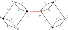
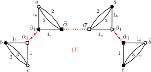
Figure 18: Graphical decomposition for the simpler melonic graph of order six in D=3.

The edge-cut $\mathcal{I}$ is shown in Figure 18, as well as the full graphical decomposition. The successive chosen color sets are $I=\{1,2,3\}$, and $I_{1}=\{1_{b},1_{c}\}$. Also, $J_{1}=\{1_{b}\}$, $\tilde{J}_{1}=\{2_{a},3_{a}\}$, and $J_{2}=\{2_{c},3_{c}\}$. The expression of the partition function corresponding to these choices is

$$Z_{\mathcal{B}^{1}}(\lambda,N)=\int d\mu^{c}(T)d\mu^{c}(\sigma)d\mu^{c}_{X}(\alpha_{1},\beta_{1})e^{ig_{\mathcal{B}^{1}}\bigl{(}[\bar{T}._{\tilde{J}_{1}}\sigma]._{I_{1}}\beta_{1}+g_{\mathcal{B}^{1}}[\bar{T}._{J_{2}}T]._{I_{1}}\alpha_{1}+c.c.\bigr{)}}.$$ (155)

After the $\sigma$ integration, one obtains

$$Z_{\mathcal{B}^{1}}(\lambda,N) = \int d\mu^{c}(T)d\mu^{c}_{X}(\alpha_{1},\beta_{1})e^{g_{\mathcal{B}^{1}}^{2}\bigl{(}i[\bar{T}._{J_{2}}T]._{I_{1}}\alpha_{1}+c.c.-[\bar{T}._{1_{b}}\beta_{1}]._{I}[\bar{\beta}_{1}._{1_{b}}T]\bigr{)}}$$ (156)

$$= \int d\mu^{c}(T)d\mu^{c}_{X}(\alpha_{1},\beta_{1})e^{g_{\mathcal{B}^{1}}^{2}\bar{T}._{\llbracket 1,D\rrbracket}\bigl{(}i(\alpha_{1}+\alpha_{1}^{\dagger})\otimes\mathds{1}^{\otimes(2)}-[\bar{\beta}_{1}._{1_{c}}\beta_{1}]\otimes\mathds{1}^{\otimes(2)}\bigr{)}._{\llbracket 1,D\rrbracket}T},$$ (157)

so that, taking into account that $\alpha_{1}$ and $\beta_{1}$ are actually matrices with first index $1_{b}$ and second index $1_{c}$, the integration over tensor $\sigma$ gives

$$Z_{\mathcal{B}^{1}}(\lambda,N)=\int d\mu^{c}_{X}(\alpha_{1},\beta_{1})e^{-N^{2}\operatorname{Tr}\ln\bigl{[}\,\mathds{1}-\,g_{\mathcal{B}^{1}}^{2}\bigl{(}\ i(\alpha_{1}+\alpha_{1}^{\dagger})\ -\ \beta_{1}\beta_{1}^{\dagger}\bigr{)}\ \bigr{]}}.$$ (158)

With the notation of the previous sections, this model has $k=3,\,m=2,\,t=1,\,s=4$, and $u=1$. The only differences with the matrix invariant of order six are the squared factor $N^{2}$ in front of the trace and the power of $N$ in $g_{\mathcal{B}^{1}}$, leading to a different value of $u$ :

$$Z_{\mathcal{B}^{1}}(\lambda,N)=\int d\mu_{X}^{c}(\alpha_{1},\beta_{1})e^{-N^{2}\operatorname{Tr}\ln\bigl{[}{\mathds{1}}^{\otimes 4}-g_{\mathcal{B}^{1}}{\mathbb{M}}_{\mathcal{B}^{1}}(\alpha_{1},\beta_{1})\bigr{]}},\quad g_{\mathcal{B}^{1}}=\frac{\lambda^{1/6}}{N^{2/3}},\quad{\mathbb{M}}_{\mathcal{B}^{1}}=\begin{pmatrix}0&i\beta_{1}&i\alpha_{1}&i{\mathds{1}}\\ i\beta_{1}^{\dagger}&0&0&0\\ \mathds{1}&0&0&0\\ \alpha_{1}^{\dagger}&0&0&0\end{pmatrix}.$$ (159)

Here $\Theta(\mathcal{B}_{1})=2$ is optimal and the $\Theta(\mathcal{B}_{1})$ identity tensorial factors have been factorized in ${\mathbb{M}}_{\mathcal{B}^{1}}$, giving the $N^{2}$ factor.

The second type of invariant is obtained by picking two colors $c,c^{\prime}$, hence there are $d(d-1)/2$ such invariants $\mathcal{B}^{2}_{c,c^{\prime}}$. We define the $N^{2}\times N^{2}$ matrix (acting on ${\cal{H}}_{cc^{\prime}}$),

$$A_{c,c^{\prime}}(T)=[\bar{T}._{\widehat{\{c,c^{\prime}\}}}T],$$ (160)

with first indices those of $T$ left free in the above summation, and second indices the free indices of $\bar{T}$. The previously defined $A_{c}$ and $A_{c^{\prime}}$ act on ${\cal{H}}_{c}$ and ${\cal{H}}_{c^{\prime}}$, so their matrix tensor product $[A_{c}\otimes A_{c^{\prime}}]$ is a matrix also acting on ${\cal{H}}_{cc^{\prime}}$. Then $\mathcal{B}^{2}_{c,c^{\prime}}$ is defined by

$$\mathcal{B}^{2}_{c,c^{\prime}}=:\operatorname{Tr}_{cc^{\prime}}\bigl{(}[A_{c}(T)\otimes A_{c^{\prime}}(T)].A_{c,c^{\prime}}(T)\bigr{)},$$ (161)

and corresponds to the graph in the left of Figure 19 (in the case $D=3$). The associated partition function is

$$Z_{\mathcal{B}^{2}}(\lambda,N)=\int d\mu(T)e^{-\lambda N^{-4}\mathcal{B}^{2}}.$$ (162)

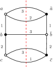
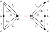
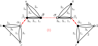
Figure 19: Graphical decomposition for the other melonic graph of order six in D=3.

We choose the edge-cut $\mathcal{I}$ ias on the left of Figure 19. The successive chosen color sets are $I=\{1_{a},2_{c},3_{a},3_{b},3_{c}\}$, and $I_{1}=\{1_{b},1_{c},3_{b},3_{c}\}$. Here, $J_{1}=\{1_{b}\}$ and $\tilde{J}_{1}=\{2_{a},3_{a}\}$, but $J_{2}=\{2_{c}\}$. The expression of the partition function corresponding to these choices is

$$Z_{\mathcal{B}^{2}}(\lambda,N)=\int d\mu^{c}(T)d\mu^{c}(\sigma)d\mu^{c}_{X}(\alpha_{1},\beta_{1})e^{ig_{\mathcal{B}^{2}}\bigl{(}[\bar{T}._{\tilde{J}_{1}}\sigma]._{I_{1}}\beta_{1}+g_{\mathcal{B}^{2}}[\bar{T}._{2_{c}}T]._{I_{1}}\alpha_{1}+c.c.\bigr{)}},$$ (163)

where now $\alpha_{1}$ and $\beta_{1}$ are rank 4 tensors. We will however understand $\alpha_{1}$ as a $N^{2}\times N^{2}$ square matrix $\alpha_{1\mid 1_{b},3_{b}\ ;\ 1_{c},3_{c}}$ and $\beta_{1}$ as a rectangular $N\times N^{3}$ matrix, $\beta_{1\mid 1_{b}\ ;\ 3_{b},1_{c},3_{c}}$. After the $\sigma$ integration, one obtains

$$Z_{\mathcal{B}^{2}}(\lambda,N) = \int d\mu^{c}(T)d\mu^{c}_{X}(\alpha_{1},\beta_{1})e^{g_{\mathcal{B}}^{2}\bigl{(}i[\bar{T}._{2_{c}}T]._{I_{1}}\alpha_{1}+c.c.-[\bar{T}._{1_{b}}\beta_{1}]._{I}[\bar{\beta}_{1}._{1_{b}}T]\bigr{)}}$$ (164)

$$= \int d\mu^{c}(T)d\mu^{c}_{X}(\alpha_{1},\beta_{1})e^{g_{\mathcal{B}}^{2}\bar{T}._{\llbracket 1,D\rrbracket}\bigl{(}i(\alpha_{1}+\bar{\alpha}_{1})\otimes\mathds{1}^{\otimes(1)}-[\bar{\beta}_{1}._{\{1_{c},3_{b},3_{c}\}}\beta_{1}]\otimes\mathds{1}^{\otimes(2)}\bigr{)}._{\llbracket 1,D\rrbracket}T},$$ (165)

$$Z_{\mathcal{B}^{2}}(\lambda,N)=\int d\mu^{c}_{X}(\alpha_{1},\beta_{1})e^{-N\operatorname{Tr}\ln\bigl{[}\,\mathds{1}-\,g_{\mathcal{B}^{2}}^{2}\bigl{(}\ i(\alpha_{1}+\alpha_{1}^{\dagger})\ -\ \beta_{1}\beta_{1}^{\dagger}\otimes\mathds{1}^{\otimes(1)}]\bigr{)}\ \bigr{]}}.$$ (166)

This example has $k=3,\,m=2,\,t=3,\,s=4$, and $u=7$. It exhibits rectangular matrices and identity factors that are not factorable, which is the case for general symmetric tensor invariants. One can express this result in terms of a linear Hermitian matrix,

$$Z_{\mathcal{B}^{2}}(\lambda,N)=\int d\mu_{X}^{c}(\alpha_{1},\beta_{1})e^{-N\operatorname{Tr}\ln\bigl{[}{\mathds{1}}^{\otimes(10)}-g_{\mathcal{B}^{2}}{\mathbb{M}}_{\mathcal{B}^{2}}(\alpha_{1},\beta_{1})\bigr{]}}\quad\mathrm{and}\quad{\mathbb{M}}_{\mathcal{B}^{2}}=\left(\begin{array}[]{cclccccccc}&\lx@intercol\hfil\hfil\lx@intercol\vrule\lx@intercol&\lx@intercol\hfil\raisebox{-8.61108pt}[5.69046pt][5.69046pt]{\makebox[56.9055pt][c]{{$i\beta_{1}\otimes\mathds{1}$}}}\hfil\lx@intercol\vrule\lx@intercol&\raisebox{-6.45831pt}[5.69046pt][5.69046pt]{\makebox[19.91684pt][r]{{$i\alpha_{1}$}}}&\lx@intercol\hfil\hfil\lx@intercol\vrule\lx@intercol&\lx@intercol\hfil i{\mathds{1}}\hfil\lx@intercol\vrule\lx@intercol&0\\ \cline{6-7}\cr&\lx@intercol\hfil\hfil\lx@intercol\vrule\lx@intercol&\lx@intercol\hfil\hfil\lx@intercol\vrule\lx@intercol&&\lx@intercol\hfil\hfil\lx@intercol\vrule\lx@intercol&\lx@intercol\hfil 0\hfil\lx@intercol\vrule\lx@intercol&i\mathds{1}\\ \hline\cr&\lx@intercol\hfil\hfil\lx@intercol\vrule\lx@intercol&\\[0.0pt] \raisebox{-8.61108pt}[5.69046pt][5.69046pt]{\makebox[8.5359pt][c]{{$\ \ \ \beta_{1}^{\dagger}\otimes\mathds{1}$}}}&\lx@intercol\hfil\hfil\lx@intercol\vrule\lx@intercol&&\raisebox{-51.6665pt}[5.69046pt][5.69046pt]{\huge\mbox{{$0$}}}\\ &\lx@intercol\hfil\hfil\lx@intercol\vrule\lx@intercol&\\[0.0pt] &\lx@intercol\hfil\hfil\lx@intercol\vrule\lx@intercol&\\[0.0pt] \cline{1-2}\cr\lx@intercol\hfil{\mathds{1}}\hfil\lx@intercol\vrule\lx@intercol&\lx@intercol\hfil 0\hfil\lx@intercol\vrule\lx@intercol\\ \cline{1-2}\cr\lx@intercol\hfil 0\hfil\lx@intercol\vrule\lx@intercol&\lx@intercol\hfil{\mathds{1}}\hfil\lx@intercol\vrule\lx@intercol\\ \cline{1-2}\cr\raisebox{-7.3194pt}[5.69046pt][5.69046pt]{\makebox[11.38092pt][r]{{$\alpha_{1}^{\dagger}$}}}&\lx@intercol\hfil\hfil\lx@intercol\vrule\lx@intercol\\ &\lx@intercol\hfil\hfil\lx@intercol\vrule\lx@intercol\end{array}\right),\quad$$

where $g_{\mathcal{B}^{2}}=\frac{\lambda^{1/6}}{N^{2/3}}$, $\Theta(\mathcal{B}_{2})=1$ is optimal and the $\Theta(\mathcal{B}_{2})$ identity tensorial factors have been factorized, giving rise to the $N$ factor before the trace. We recall that here $\beta_{1}\otimes\mathds{1}$ is a $N^{2}\times N^{4}$ matrix, and $\alpha_{1}$ a $N^{2}\times N^{2}$ matrix, $\mathds{1}$ being the $N\times N$ identity, as usual.

The previous $k=3$ examples are a bit special, in particular because all positive tensor invariants at $k=3$ are planar, and in fact melonic. We could worry what happens when the initial invariant, hence also the initial decomposition step $F.\bar{\sigma}$ is a non-planar graph. Hence in our last explicit example we treat an example of this type with $k=5$.

We consider the partition function $Z_{\mathcal{B}}(\lambda,N)=\int d\mu(T)e^{-\lambda N^{-s}\mathcal{B}},$ where $\mathcal{B}$ is represented on the left of Figure 20 together with its axis of symmetry. Note that the correct scaling $s$ for a non-trivial perturbative $1/N$ expansion for this invariant is not known. However, we know that for $s=D-1$ the $1/N$ expansion is at least defined, although possibly trivial.

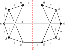
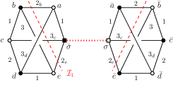
Figure 20: A non-planar positive $k=5$ tensor invariant and its initial intermediate field step.

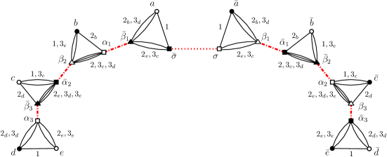
Figure 21: Full intermediate field decomposition, before integration of the field with even indices.

For this example we only provide a graphical decomposition and the resulting expression of the partition function. By looking at the triangular graphs of the intermediate field decomposition, one can read the sizes of the involved rectangular matrices, together with the colors of the spaces in which they act. As $k$ is odd in this case, the remaining fields after integration are those labeled with odd indices. One can see that $\alpha_{1}$ is $N\times N^{3}$, $\beta_{1}$ and $\alpha_{3}$ are $N^{2}\times N^{2}$, $\beta_{3}$ is $N\times N^{3}$, all acting on spaces of color 2,3. Color 1 is therefore factorable in the sum of tensor products $\ i\mathbf{H}_{\mathcal{B}}(\xi)\ -\ \eta(k)\beta_{1}\beta_{1}^{\dagger}\otimes\mathds{1}^{\otimes\lvert\tilde{J}_{1}\rvert}\,\bigr{)}$. $\Gamma(\mathcal{B})$ is $3\times 3+5+5+5=24$, and the factorization of the identity acting on color 1 leaves a size $\Gamma-(k+1)\times\Theta=24-6\times 1=18$ linear matrix,

$$Z_{\mathcal{B}}(\lambda,N)=\int d\mu_{X}^{c}(\alpha_{1},\beta_{1})d\mu_{X}^{c}(\alpha_{3},\beta_{3})e^{-N\operatorname{Tr}\ln\bigl{[}{\mathds{1}}^{\otimes(18)}-g_{\mathcal{B}}{\mathbb{M}}_{\mathcal{B}}\bigr{]}},\quad g_{\mathcal{B}}=(\lambda N^{-s})^{1/10},$$ (167)

$$\mathbb{M}_{\mathcal{B}}=\left(\begin{array}[]{cclccccccccccccc}&\lx@intercol\hfil\hfil\lx@intercol\vrule\lx@intercol&\lx@intercol\hfil\raisebox{-8.61108pt}[5.69046pt][5.69046pt]{\makebox[56.9055pt][c]{{$i\beta_{1}\otimes\mathds{1}$}}}\hfil\lx@intercol\vrule\lx@intercol&\lx@intercol\hfil\raisebox{-8.61108pt}[5.69046pt][5.69046pt]{\makebox[56.9055pt][c]{{$i\alpha_{1}\otimes\mathds{1}$}}}\hfil\lx@intercol\vrule\lx@intercol&\lx@intercol\hfil\raisebox{-8.61108pt}[5.69046pt][5.69046pt]{\makebox[56.9055pt][c]{{$i\beta_{3}\otimes\mathds{1}$}}}\hfil\lx@intercol\vrule\lx@intercol&\lx@intercol\hfil\raisebox{-6.45831pt}[5.69046pt][5.69046pt]{\makebox[34.14322pt][c]{{$i\alpha_{3}$}}}\hfil\lx@intercol\vrule\lx@intercol&\lx@intercol\hfil i{\mathds{1}}\hfil\lx@intercol\vrule\lx@intercol&0\\ \cline{7-8}\cr&\lx@intercol\hfil\hfil\lx@intercol\vrule\lx@intercol&\lx@intercol\hfil\hfil\lx@intercol\vrule\lx@intercol&\lx@intercol\hfil\hfil\lx@intercol\vrule\lx@intercol&\lx@intercol\hfil\hfil\lx@intercol\vrule\lx@intercol&\lx@intercol\hfil\hfil\lx@intercol\vrule\lx@intercol&\lx@intercol\hfil 0\hfil\lx@intercol\vrule\lx@intercol&i\mathds{1}\\ \hline\cr&\lx@intercol\hfil\hfil\lx@intercol\vrule\lx@intercol&\\[0.0pt] \raisebox{-8.61108pt}[5.69046pt][5.69046pt]{\makebox[8.5359pt][c]{{$\ \ \ \beta_{1}^{\dagger}\otimes\mathds{1}$}}}&\lx@intercol\hfil\hfil\lx@intercol\vrule\lx@intercol\\ &\lx@intercol\hfil\hfil\lx@intercol\vrule\lx@intercol&\\[0.0pt] &\lx@intercol\hfil\hfil\lx@intercol\vrule\lx@intercol&\\[0.0pt] \cline{1-2}\cr&\lx@intercol\hfil\hfil\lx@intercol\vrule\lx@intercol&\\[0.0pt] \raisebox{-8.61108pt}[5.69046pt][5.69046pt]{\makebox[8.5359pt][c]{{$\ \ \ \beta_{3}^{\dagger}\otimes\mathds{1}$}}}&\lx@intercol\hfil\hfil\lx@intercol\vrule\lx@intercol&&\raisebox{-51.6665pt}[5.69046pt][5.69046pt]{\huge\mbox{{$0$}}}\\ &\lx@intercol\hfil\hfil\lx@intercol\vrule\lx@intercol&\\[0.0pt] &\lx@intercol\hfil\hfil\lx@intercol\vrule\lx@intercol&\\[0.0pt] \cline{1-2}\cr&\lx@intercol\hfil\hfil\lx@intercol\vrule\lx@intercol&\\[0.0pt] \raisebox{-8.61108pt}[5.69046pt][5.69046pt]{\makebox[8.5359pt][c]{{$\ \ \ \alpha_{1}^{\dagger}\otimes\mathds{1}$}}}&\lx@intercol\hfil\hfil\lx@intercol\vrule\lx@intercol\\ &\lx@intercol\hfil\hfil\lx@intercol\vrule\lx@intercol&\\[0.0pt] &\lx@intercol\hfil\hfil\lx@intercol\vrule\lx@intercol&\\[0.0pt] \cline{1-2}\cr\lx@intercol\hfil{\mathds{1}}\hfil\lx@intercol\vrule\lx@intercol&\lx@intercol\hfil 0\hfil\lx@intercol\vrule\lx@intercol\\ \cline{1-2}\cr\lx@intercol\hfil 0\hfil\lx@intercol\vrule\lx@intercol&\lx@intercol\hfil{\mathds{1}}\hfil\lx@intercol\vrule\lx@intercol\\ \cline{1-2}\cr\raisebox{-7.3194pt}[5.69046pt][5.69046pt]{\makebox[11.38092pt][r]{{$\alpha_{3}^{\dagger}$}}}&\lx@intercol\hfil\hfil\lx@intercol\vrule\lx@intercol\\ &\lx@intercol\hfil\hfil\lx@intercol\vrule\lx@intercol\end{array}\right).\quad$$ (186)

For $s=D-1=2$, we obtain $k=5,\,m=4,\,t=3$, and $u=7$.

References

- (1) Constructive quantum field theory, Springer Lecture Notes in Physics 25, 1973
- (2) J. Glimm and A. Jaffe, Quantum Physics, A Functional Integral Point of View, Springer 1987
- (3) V. Rivasseau, From Perturbative to Constructive Renormalization, Princeton University Press 1991.
- (4) J.-P. Eckmann, J. Magnen and R. Sénéor, “Decay properties and Borel summability for the Schwinger functions in theories”, Comm. Math. Phys. 39, 251 (1974).
- (5) J. Magnen and R. Sénéor, “Phase space cell expansion and Borel summability for the Euclidean theory”, Comm. Math. Phys. 56, 237 (1977).
- (6) J. Feldman, J. Magnen, V. Rivasseau and R. Sénéor, “A Renormalizable Field Theory: The Massive Gross-Neveu Model in Two-dimensions,” Commun. Math. Phys. 103, 67 (1986). doi:10.1007/BF01464282
- (7) V. Rivasseau, “The Tensor Track, III,” Fortsch. Phys. 62, 81 (2014) [arXiv:1311.1461 [hep-th]].
- (8) T. E. Regge ”General relativity without coordinates”. Nuovo Cim. 19 558–571, (1961).
- (9) J. Ambjorn, “Simplicial Euclidean and Lorentzian Quantum Gravity”, arXiv:gr-qc/0201028.
- (10) R. Loll, J. Ambjorn and J. Jurkiewicz, “The Universe from Scratch”, Contemp.Phys. 47 (2006) 103-117, hep-th/0509010,
- (11) J. Ambjorn, A. Görlich, J. Jurkiewicz and R. Loll, “Causal dynamical triangulations and the search for a theory of quantum gravity,” Int. J. Mod. Phys. D 22, 1330019 (2013).
- (12) D. V. Boulatov, “A Model of three-dimensional lattice gravity,” Mod. Phys. Lett. A 7, 1629 (1992), hep-th/9202074.
- (13) L. Freidel, “Group field theory: An overview,” Int. J. Theor. Phys. 44, 1769 (2005), arXiv:hep-th/0505016.
- (14) T. Krajewski, “Group field theories,” PoS QGQGS 2011, 005 (2011), arXiv:1210.6257.
- (15) J. Ben Geloun, J. Magnen and V. Rivasseau, “Bosonic Colored Group Field Theory,” Eur. Phys. J. C 70, 1119 (2010), arXiv:0911.1719.
- (16) F. David, “A Model of Random Surfaces with Nontrivial Critical Behavior,” Nucl. Phys. B 257, 543 (1985).
- (17) V. A. Kazakov, “Bilocal Regularization of Models of Random Surfaces,” Phys. Lett. B 150, 282 (1985).
- (18) P. Di Francesco, P. H. Ginsparg and J. Zinn-Justin, “2-D Gravity and random matrices,” Phys. Rept. 254, 1 (1995) [hep-th/9306153].
- (19) H. Grosse and R. Wulkenhaar, “Renormalisation of phi**4 theory on noncommutative R**4 in the matrix base,” Commun. Math. Phys. 256, 305 (2005), arXiv:hep-th/0401128.
- (20) H. Grosse and R. Wulkenhaar, “The beta function in duality covariant noncommutative phi**4 theory,” Eur. Phys. J. C 35, 277 (2004), hep-th/0402093.
- (21) M. Disertori and V. Rivasseau, “Two and three loops beta function of non commutative Phi(4)**4 theory,” Eur. Phys. J. C 50, 661 (2007), hep-th/0610224.
- (22) M. Disertori, R. Gurau, J. Magnen and V. Rivasseau, “Vanishing of Beta Function of Non Commutative Phi**4(4) Theory to all orders,” Phys. Lett. B 649, 95 (2007), hep-th/0612251.
- (23) H. Grosse and R. Wulkenhaar, “Progress in solving a noncommutative quantum field theory in four dimensions,” arXiv:0909.1389.
- (24) H. Grosse and R. Wulkenhaar, “Self-dual noncommutative -theory in four dimensions is a non-perturbatively solvable and non-trivial quantum field theory,” arXiv:1205.0465.
- (25) H. Grosse and R. Wulkenhaar, “Solvable 4D noncommutative QFT: phase transitions and quest for reflection positivity,” arXiv:1406.7755 [hep-th].
- (26) H. Grosse and R. Wulkenhaar, “On the fixed point equation of a solvable 4D QFT model,” arXiv:1505.05161 [math-ph].
- (27) J. Ambjorn, B. Durhuus and T. Jonsson, “Three-Dimensional Simplicial Quantum Gravity And Generalized Matrix Models, Mod. Phys. Lett. A 6, 1133 (1991).
- (28) N. Sasakura, “Tensor model for gravity and orientability of manifold, Mod. Phys. Lett. A 6, 2613 (1991).
- (29) M. Gross, “Tensor models and simplicial quantum gravity in 2-D, Nucl. Phys. Proc. Suppl. 25A, 144 (1992).
- (30) G. ’t Hooft, “A PLANAR DIAGRAM THEORY FOR STRONG INTERACTIONS,” Nucl. Phys. B 72, 461 (1974).
- (31) R. Gurau, “Colored Group Field Theory,” Commun. Math. Phys. 304, 69 (2011) doi:10.1007/s00220-011-1226-9 [arXiv:0907.2582 [hep-th]].
- (32) R. Gurau and J. P. Ryan, “Colored Tensor Models - a review,” SIGMA 8, 020 (2012) doi:10.3842/SIGMA.2012.020 [arXiv:1109.4812 [hep-th]].
- (33) R. Gurau, “Universality for Random Tensors,” Ann. Inst. H. Poincare Probab. Statist. 50, no. 4, 1474 (2014) doi:10.1214/13-AIHP567 [arXiv:1111.0519 [math.PR]].
- (34) V. Bonzom, R. Gurau and V. Rivasseau, “Random tensor models in the large N limit: Uncoloring the colored tensor models,” Phys. Rev. D 85, 084037 (2012) doi:10.1103/PhysRevD.85.084037 [arXiv:1202.3637 [hep-th]].
- (35) R. Gurau, “The 1/N expansion of colored tensor models,” Annales Henri Poincare 12, 829 (2011) doi:10.1007/s00023-011-0101-8 [arXiv:1011.2726 [gr-qc]].
- (36) R. Gurau and V. Rivasseau, “The 1/N expansion of colored tensor models in arbitrary dimension,” Europhys. Lett. 95, 50004 (2011) doi:10.1209/0295-5075/95/50004 [arXiv:1101.4182 [gr-qc]].
- (37) R. Gurau, “The complete 1/N expansion of colored tensor models in arbitrary dimension,” Annales Henri Poincare 13, 399 (2012) doi:10.1007/s00023-011-0118-z [arXiv:1102.5759 [gr-qc]].
- (38) V. Bonzom, “New 1/N expansions in random tensor models,” JHEP 1306, 062 (2013) doi:10.1007/JHEP06(2013)062 [arXiv:1211.1657 [hep-th]].
- (39) V. Bonzom, T. Delepouve and V. Rivasseau, “Enhancing non-melonic triangulations: A tensor model mixing melonic and planar maps,” Nucl. Phys. B 895, 161 (2015) doi:10.1016/j.nuclphysb.2015.04.004 [arXiv:1502.01365 [math-ph]].
- (40) V. Bonzom, “Large limits in tensor models: Towards more universality classes of colored triangulations in dimension ,” arXiv:1603.03570 [math-ph].
- (41) J. Ben Geloun and V. Rivasseau, “A Renormalizable 4-Dimensional Tensor Field Theory,” arXiv:1111.4997.
- (42) J. Ben Geloun and V. Rivasseau, “Addendum to ’A Renormalizable 4-Dimensional Tensor Field Theory’,” Commun. Math. Phys. 322, 957 (2013), arXiv:1209.4606.
- (43) D. O. Samary and F. Vignes-Tourneret, “Just Renormalizable TGFT’s on with Gauge Invariance,” arXiv:1211.2618.
- (44) S. Carrozza, D. Oriti and V. Rivasseau, “Renormalization of Tensorial Group Field Theories: Abelian U(1) Models in Four Dimensions,” arXiv:1207.6734.
- (45) S. Carrozza, D. Oriti and V. Rivasseau, “Renormalization of an SU(2) Tensorial Group Field Theory in Three Dimensions,” arXiv:1303.6772.
- (46) J. Ben Geloun, “Renormalizable Models in Rank Tensorial Group Field Theory,” arXiv:1306.1201.
- (47) J. Ben Geloun and D. O. Samary, “3D Tensor Field Theory: Renormalization and One-loop -functions,” Annales Henri Poincare 14, 1599 (2013), arXiv:1201.0176.
- (48) J. Ben Geloun, “Two and four-loop -functions of rank 4 renormalizable tensor field theories,” Class. Quant. Grav. 29, 235011 (2012), arXiv:1205.5513.
- (49) J. Ben Geloun, “Asymptotic Freedom of Rank 4 Tensor Group Field Theory,” arXiv:1210.5490.
- (50) D. O. Samary, “Beta functions of gauge invariant just renormalizable tensor models,” arXiv:1303.7256.
- (51) V. Rivasseau, “Why are tensor field theories asymptotically free?,” Europhys. Lett. 111, no. 6, 60011 (2015) doi:10.1209/0295-5075/111/60011 [arXiv:1507.04190 [hep-th]].
- (52) V. Rivasseau, “Constructive Tensor Field Theory,” arXiv:1603.07312 [math-ph].
- (53) V. Rivasseau, “Constructive Matrix Theory,” JHEP 0709, 008 (2007) doi:10.1088/1126-6708/2007/09/008 [arXiv:0706.1224 [hep-th]].
- (54) J. Magnen, K. Noui, V. Rivasseau and M. Smerlak, “Scaling behaviour of three-dimensional group field theory,” Class. Quant. Grav. 26 (2009) 185012 [arXiv:0906.5477 [hep-th]].
- (55) R. Gurau, “The 1/N Expansion of Tensor Models Beyond Perturbation Theory,” Commun. Math. Phys. 330, 973 (2014) [arXiv:1304.2666 [math-ph]].
- (56) T. Delepouve, R. Gurau and V. Rivasseau, “Universality and Borel Summability of Arbitrary Quartic Tensor Models,” arXiv:1403.0170 [hep-th].
- (57) R. Gurau and T. Krajewski, “Analyticity results for the cumulants in a random matrix model,” arXiv:1409.1705 [math-ph].
- (58) J. Magnen and V. Rivasseau, “Constructive field theory without tears,” Annales Henri Poincare 9 (2008) 403 [arXiv:0706.2457 [math-ph]].
- (59) V. Rivasseau and Z. Wang, “How to Resum Feynman Graphs,” Annales Henri Poincaré 15, no. 11, 2069 (2014) [arXiv:1304.5913 [math-ph]].
- (60) D. Brydges and T. Kennedy, Mayer expansions and the Hamilton-Jacobi equation, Journal of Statistical Physics, 48, 19 (1987).
- (61) A. Abdesselam and V. Rivasseau, “Trees, forests and jungles: A botanical garden for cluster expansions,” arXiv:hep-th/9409094.
- (62) T. Delepouve and V. Rivasseau, “Constructive Tensor Field Theory: The Model,” arXiv:1412.5091 [math-ph].
- (63) V. Lahoche, “Constructive Tensorial Group Field Theory I:The Model,” arXiv:1510.05050 [hep-th].
- (64) V. Lahoche, “Constructive Tensorial Group Field Theory II: The Model,” arXiv:1510.05051 [hep-th].
- (65) R. Gurau and V. Rivasseau, “The Multiscale Loop Vertex Expansion,” Annales Henri Poincaré 16, no. 8, 1869 (2015) [arXiv:1312.7226 [math-ph]].
- (66) V. Bonzom, “Multicritical tensor models and hard dimers on spherical random lattices,” Phys. Lett. A 377, 501 (2013) doi:10.1016/j.physleta.2012.12.022 [arXiv:1201.1931 [hep-th]].
- (67) V. Bonzom, L. Lionni and V. Rivasseau, “Colored triangulations of arbitrary dimensions are stuffed Walsh maps”, arXiv:1508.03805.
- (68) L. Lionni and V. Rivasseau, ‘Note on the Intermediate Field Representation of Theory in Zero Dimension”, arXiv:1601.02805.
- (69) E. Caliceti, M. Meyer-Hermann, P. Ribeca, A. Surzhykov and U. D. Jentschura, “From Useful Algorithms for Slowly Convergent Series to Physical Predictions Based on Divergent Perturbative Expansions,” Phys. Rept. 446 (2007) 1 [arXiv:0707.1596 [physics.comp-ph]].
- (70) A. D. Sokal, “An Improvement Of Watson’s Theorem On Borel Summability,” J. Math. Phys. 21, 261 (1980).
- (71) M. Ferri and C. Gagliardi, “Crystallization moves”, Pacific J. Math. 100 (1982) 85-103.
- (72) M. Ferri, C. Gagliardi and L. Grasselli, “A graph-theoretical representation of PL-manifolds - A survey on crystallizations,” Aequationes Mathematicae, 31, 121-141(1986).
- (73) S. Lins, “Gems, computers and attractors for 3-manifolds”, Series on Knots and Everything, Vol. 5, World Scientific Publishing Co. Inc., River Edge, NJ, 1995.