The Razor’s Edge of Collapse: The Transition Point from Lognormal to Powerlaw in Molecular Cloud PDFs

Abstract

We derive an analytic expression for the transitional column density value ($s_{t}$) between the lognormal and power-law form of the probability distribution function (PDF) in star-forming molecular clouds. Our expression for $s_{t}$ depends on the mean column density, the variance of the lognormal portion of the PDF, and the slope of the power-law portion of the PDF. We show that $s_{t}$ can be related to physical quantities such as the sonic Mach number of the flow and the power-law index for a self-gravitating isothermal sphere. This implies that the transition point between the lognormal and power-law density/column density PDF represents the critical density where turbulent and thermal pressure balance, the so-called “post-shock density.” We test our analytic prediction for the transition column density using dust PDF observations reported in the literature as well as numerical MHD simulations of self-gravitating supersonic turbulence with the Enzo code. We find excellent agreement between the analytic $s_{t}$ and the measured values from the numerical simulations and observations (to within 1.5 A_V). We discuss the utility of our expression for determining the properties of the PDF from unresolved low density material in dust observations, for estimating the post-shock density, and for determining the HI-H₂ transition in clouds.

1. Introduction

Star formation in galaxies occurs in dense molecular environments and is governed by the complex interaction of gravity, magnetic fields, turbulence, and radiation pressure (McKee & Ostriker, 2007; Elmegreen, 2011). Despite decades of study, the fundamental conditions behind the transition of diffuse atomic gas to cold molecular gas are still relatively unconstrained (Sternberg, 1988; Krumholz et al., 2009; McKee & Krumholz, 2010; Bialy et al., 2015). The initial conditions imprinted on the diffuse and molecular gas on parsec scales (i.e. the level of turbulence, the cloud density, the structure of the magnetic field) may determine the key properties of the initial mass function (IMF) and the star formation rates in galaxies (Hennebelle & Chabrier, 2011). Therefore the properties of diffuse and molecular gas in and around star-forming clouds must be quantified in order to construct a theory of star formation that predicts the IMF.

The density and column density probability distribution functions (PDFs) have been used extensively in understanding the properties of galactic gas dynamics, from the diffuse ionized medium to dense star-forming clouds. The application of the PDF in molecular clouds has included density tracers such as CO (Lee et al., 2012; Burkhart et al., 2013b) and dust (Kainulainen et al., 2009; Froebrich & Rowles, 2010; Schneider et al., 2013, 2014, 2015; Lombardi et al., 2015). Tracing the PDF using dust emission and absorption provides the largest dynamic range of densities, in contrast to molecular line tracers such as CO, which suffer from depletion and opacity effects (Goodman et al., 2009; Burkhart et al., 2013b, a).

Simulations of self-gravitating MHD turbulence have successfully reproduced the shape and properties of the observational PDFs (Burkhart et al., 2009; Federrath & Klessen, 2012, 2013; Collins et al., 2012; Burkhart et al., 2015) suggesting that the gas PDF stems from a combination of turbulence (which induces a lognormal PDF shape in density) and self-gravity (which is characterized by a power-law PDF in density). In more detail, observed and simulated PDFs of Giant Molecular Cloud (GMC) environments, which include supersonic turbulence and self-gravity, suggest that the highest column density regime of the PDF (i.e., above column densities of 1 A_V) has a power-law distribution (Collins et al., 2011; Schneider et al., 2013; Lombardi et al., 2015; Burkhart et al., 2009; Federrath & Klessen, 2012, 2013; Collins et al., 2012; Burkhart et al., 2015) while the lower column density material in the PDF is dominated by turbulent diffuse gas and takes on a lognormal form (Vazquez-Semadeni, 1994; Burkhart & Lazarian, 2012; Padoan et al., 1997).

The implications for the shape of the gas density PDF in ISM clouds are profoundly linked to the kinematics, star formation rates and the chemistry of the gas (Federrath & Klessen, 2012). Kinematically, the PDF width of the lognormal density distribution can be related to the sonic Mach number of the gas in an isothermal cloud (Federrath et al., 2008; Burkhart et al., 2009; Kainulainen & Tan, 2013; Burkhart & Lazarian, 2012; Burkhart et al., 2015). Star formation rates are linked to the gas density PDF in several analytic models which use the high density end of the PDF to provide the dense gas fraction to calculate star formation efficiencies (Krumholz & McKee, 2005; Hennebelle & Chabrier, 2011; Padoan & Nordlund, 2011). More recently, the HI PDF in and around GMCs has been proposed as a tracer of the HI-H₂ transition (Burkhart et al., 2015; Imara & Burkhart, 2016) as well as a more accurate tracer of the low density lognormal shape as opposed to dust emission/absorption data, which have difficulty tracing the lognormal form (Lombardi et al., 2015; Schneider et al., 2013). Burkhart et al. (2015) and Imara & Burkhart (2016) have shown that the lognormal portion of the column density PDF in a sample of Milky Way GMCs is comprised of mostly atomic HI gas while the power-law tail is built up by the molecular H₂. These studies suggest that the transition point in the column density PDF between the lognormal and power-law portions of the column density PDF traces important physical processes, such as the HI-H₂ transition and the density regime where self-gravity becomes dynamically important.

In this work we derive an analytic formula for the transitional column density from the lognormal portion of the PDF to the power-law form (denoted $s_{t}$). We organize the paper as follows. In Section 2 we derive an expression for the transitional column density for a piecewise lognormal and power-law PDF distribution based on the assumption that the PDF is continuous and differentiable. We further demonstrate that $s_{t}$ is related to the physical parameters such as the sonic Mach number of the gas (i.e. kinematics), the post-shock density, and the power-law index for a self-gravitating isothermal sphere. In Section 3 we compare our analytic expression for the transitional column density to numerical simulations of self-gravitating MHD turbulence run using the Enzo code. In Section 4 we compare our analytic expression for the transitional column density to observations using data from the literature. In Section 5 we discuss our results, followed by our conclusions in Section 6.

2. The Transition from Lognormal to Power Law Tail in the PDF of a Turbulent Self-gravitating Medium

The lognormal PDF of the gas column density is defined as

$$p_{s}(s)=\frac{1}{\sqrt{2\pi\sigma_{s}^{2}}}\exp\left(-\frac{(s-s_{0})^{2}}{2\sigma_{s}^{2}}\right)\,,$$ (1)

with $s$ the logarithm of the normalized column density:

$$s\equiv\ln{(\Sigma/\Sigma_{0})}\,.$$ (2)

The PDF is a normal distribution in $s$, meaning that it is a lognormal distribution in $\Sigma$. The quantities $\Sigma_{0}$ and $s_{0}$ denote, respectively, the mean column density and mean logarithmic column density, the latter of which can be related to the standard deviation $\sigma_{s}$ by:

$$s_{0}=-\frac{1}{2}\sigma_{s}^{2}$$ (3)

The lognormal form of the PDF of column density describes the behavior of diffuse HI and ionized gas (Berkhuijsen & Fletcher, 2008; Hill et al., 2008; Burkhart et al., 2010) as well as some star-forming molecular clouds that are not actively star-forming, e.g. see Kainulainen & Tan (2013); Schneider et al. (2013).

The PDF of the highest column density regime of self-gravitating turbulent clouds has a power-law distribution as demonstrated in numerical simulations (Federrath & Klessen, 2012, 2013; Collins et al., 2012; Burkhart et al., 2015) and observations (Kainulainen et al., 2009; Froebrich & Rowles, 2010; Schneider et al., 2013, 2015; Lombardi et al., 2015; Burkhart et al., 2015)

Based on the aforementioned numerical and observational studies, hereafter we consider a piece-wise form for the PDF of column density (similar to the assumption of Collins et al. 2012 for the 3D density) which has a lognormal distribution below a transitional column density value, denoted $s_{t}=\ln(\Sigma_{t}/\Sigma_{0})$, where $\Sigma_{t}$ is the transitional column density value. At column densities greater than $s_{t}$ the PDF is a power-law. We have

$$p_{s}(s)=\begin{cases}N\frac{1}{\sqrt{2\pi}\sigma_{s}}\exp\left[-\frac{(s-s_{0})^{2}}{2\sigma_{s}^{2}}\right],&s<s_{t}\\ Np_{0}\exp\left[{-\alpha s}\right],&s>s_{t},\end{cases}$$ (4)

where again, $s_{0}=-\frac{1}{2}\,\sigma_{s}^{2}$ and $p_{0}$ is the power-law’s amplitude where it joins the lognormal.

Here the normalization $N$ is determined by the normalization criterion, $\int_{-\infty}^{\infty}p_{s}(s)ds=1$, and is

$$N=\left(p_{0}/\alpha e^{-\alpha s_{t}}+\frac{1}{2}\left[1+{\rm erf}\left(\frac{2s_{t}+\sigma_{s}^{2}}{2^{3/2}\sigma_{s}}\right)\right]\right)^{-1}$$ (5)

If we assume that $p_{s}(s)$ is continuous and differentiable, we can formulate an analytic estimate for $\mathrm{s}_{t}$. By setting the two parts of equation (4) equal at $s_{t}$ and setting their derivatives equal, we find

$$s_{t} =\frac{1}{2}(2|\alpha|-1)\sigma_{s}^{2}$$ (6)

The transition column density value between the lognormal and power-law PDFs therefore depends on the slope of the power-law tail ($\alpha$), the standard deviation of the lognormal ($\sigma_{s}$) and the mean column density, i.e. because $s_{t}=\ln(\Sigma_{t}/\Sigma_{0})$ . We note that the solution to the transition point should be applicable (and take the same form) for both density (see Collins et al. 2012) and column density distributions since both density and column density share the same lognormal + power-law form of the PDF. In the following subsection we provide a physical interpretation for $s_{t}$.

2.1. Physical Interpretation of $s_{t}$

The transitional column density $s_{t}$ is not necessarily a criterion for a critical star-formation density, which most likely is farther out in the power-law tail. Rather, $s_{t}$ represents a transitional point between the dominance of supersonic turbulence in the cloud gas dynamics, which builds the lognormal distribution, to densities where gravity plays an increasingly important role in shaping the distribution.

Given the analytic solution for the transition point of the PDF between the lognormal and power-law tail we are now in a position to relate the properties of the transition point to the physics of the gas in a GMC. The width of the lognormal PDF ($\sigma_{s}$) depends on the properties of the turbulence in the GMC, with the primary dependence being on the sonic Mach number. For column density maps Burkhart & Lazarian (2012) relate the sonic Mach number to PDF width as:

$$\sigma_{s}^{2}=A\ln[1+b^{2}M_{s}^{2}]$$ (7)

$A=0.11$ is a scaling constant from density to column density. The forcing parameter $b$ varies from $b\approx 1/3$ for purely solenoidal (divergence-free) forcing to $b=1$ for purely compressive (curl-free) forcing of MHD turbulence (Federrath et al., 2008).

Equation 7 was shown to depend very weakly on the magnetic field (Burkhart & Lazarian, 2012). For the 3D density PDF in super-Alfvénic turbulence, Molina et al. (2012) formulated the dependency on the plasma $\beta_{0}$, i.e. the ratio of the gas pressure to magnetic pressure, as

$$\sigma_{\ln\rho/\rho_{0}}^{2}=\ln[1+b^{2}M_{s}^{2}\beta_{0}/(\beta_{0}+1)]$$ (8)

For the case of the column density, we can thus express the transition point in terms of the sonic Mach number by combining equations 6 and 7 to find

$$s_{t}=\frac{1}{2}(2|\alpha|-1)(A\ln[1+b^{2}M_{s}^{2}])$$ (9)

The transition density or column density can be further expressed in terms of the post-shock density, $\rho_{\rm{ps}}=\rho_{0}M_{s}^{2}$, which is the density at which the turbulent energy density is equal to the thermal pressure:

$$P_{therm}=\rho_{\rm{ps}}c_{s}^{2}=\rho_{0}v^{2}.$$ (10)

Manipulating this relation we find that $M_{s}^{2}=\rho_{\rm{ps}}/\rho_{0}$, meaning equation 9 becomes

$$s_{t}=(|\alpha|-1/2)A\ln[1+b^{2}\frac{\rho_{\rm{ps}}}{\rho_{0}}]$$ (11)

In the limit of strong collapse, $|\alpha|$ tends to 1.5 (see Figure 2), so the $(|\alpha|-1/2)$ term is of order unity.

Therefore,

$$\ln(\Sigma_{t}/\Sigma_{0})\approx A\ln[1+b^{2}\frac{\rho_{\rm{ps}}}{\rho_{0}}]$$ (12)

and so

$$\Sigma_{t}/\Sigma_{0}\approx(1+b^{2}\frac{\rho_{\rm{ps}}}{\rho_{0}})^{A}.$$ (13)

In the case of a 3D density field (relevant for simulations) we can express the transition density in the same form at the column density (i.e. using Equation 6) the transition density can be expressed (using Equation 8) as:

$$\rho_{t}/\rho_{0}\approx(1+b^{2}\frac{\rho_{\rm{ps}}}{\rho_{0}}\frac{\beta_{0}}{\beta_{0}+1})$$ (14)

as the exponent $A$ in Equation 13 accounts for line-of-sight (LOS) effects and radiative transfer in column density (see Burkhart et al. 2013a).

The slope of the power-law tail, $\alpha$, does not have a clear relation to other physical quantities. It depends on the collapse state of the gas, the magnetic pressure, and the LOS (Kritsuk et al., 2011; Ballesteros-Paredes et al., 2011; Collins et al., 2012; Federrath & Klessen, 2013; Burkhart et al., 2015).

In the case where the tail is produced only due to gravitational collapse, and if we assume spherical symmetry, the PDF slope of the power-law tail is related to the exponent $\gamma$ of the radial density profile $\rho\sim r^{-\gamma}$ (e.g. Shu, 1977). Girichidis et al. (2014) showed analytically that column density power-law-tail slopes of $\alpha=-2.1$ correspond to the $\gamma=2$ prediction for a collapsing isothermal sphere since $\alpha=-2/(\gamma-1)$.

3. Numerical Simulations

3.1. Numerical Parameters and Methods

We are now in a position to test the analytic relation for the transitional column density given in Equation 6. For this purpose we use simulation data generated by solving the ideal MHD equations including self-gravity using the AMR (Adaptive Mesh Refinement) code Enzo developed by Collins et al. (2010). These simulations use a root grid of $128^{3}$ with four levels of refinement to yield an effective resolution of $2048^{3}$. The Virial parameter $\alpha_{vir}$, sonic Mach number $\mathcal{M}_{s}$, and mean ratio of thermal to magnetic pressure $\beta_{0}$ are chosen here to be:

$$\alpha_{vir}=1$$

$$\mathcal{M}_{s}=9$$

$$\beta_{0}=0.2,2.0,20.0$$

which scale to physical clouds with free-fall time $t_{ff}$, box size $L_{0}$, rms velocity $v_{rms}$, total mass $M$ and mean magnetic field $B_{0}$ of:

$$t_{ff}=1.1\;{\rm Myr}$$

$$L_{0}=4.6\;{\rm pc}$$

$$v_{rms}=1.8\;{\rm km/s}$$

$$M=5900\;M_{\odot}$$

$$B_{0}=(13,4.4,1.3)\mu G.$$

These simulations start with the same initial conditions as the simulations of Collins et al. (2012), though they are down-sampled to the lower root grid resolution. Also the simulations of Collins et al. (2012) were driven during the collapse, while the present simulations were not.

These simulations have a post-shock density $\rho_{\rm{ps}}/\rho_{0}=81$. The density may also be scaled physically using $\rho_{0}=1000\ {\rm cm}^{-3}$ yielding a post-shock density of $\rho_{\rm{ps}}=8.1\times 10{{}^{4}}\ {\rm cm}^{-3}$ or a column density of $\Sigma_{\rm{ps}}=6.7\times 10^{23}\ {\rm cm}^{-2}$ given a cloud size of 4.6$\;{\rm pc}$. Typical observational values for the post-shock density range from $300\ {\rm cm}^{-3}$ to greater than $4\times 10^{4}\ {\rm cm}^{-3}$ (Li et al., 2015).

3.2. Column Density PDFs

We project the 3D density into column density along three different lines of sight (denoted $x,y,$ and $z$). A histogram is then generated of the logarithm of the normalized column density, i.e., $s=\ln(\Sigma/\Sigma_{0})$. Based on previous numerical studies (e.g., Collins et al. 2012; Burkhart et al. 2015) and the form of the PDF presented in Equation 4, we expect these simulations to show a lognormal column density PDF around the mean column density with a power-law tail developing at higher densities. We fit a lognormal to column densities within 20 percent of the peak of the distribution (to minimize contamination from the tail) and a power-law in the higher density regions where the lognormal fit begins to fail.

We show the PDF and the lognormal fits of the simulated column density at snapshot t=$0.6t_{ff}$ in Figure 1. The width of the lognormal $\sigma_{s}$ and power-law slope $\alpha$ are determined as free parameters of the fits while the transition point $s_{t}$ of the PDF is determined by finding where the least squares between the power-law fit and the data gets better than that of the lognormal fit. In Figure 1 the transition point $s_{t}$ is indicated by a green dot, the lognormal fit is a red line, the power-law a black line and the actual data a blue line.

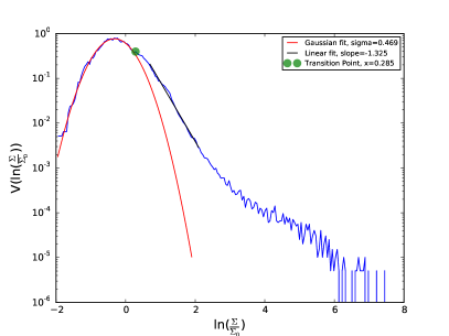
Figure 1.— An example PDF shown at $0.6t_{ff}$ for $\beta_{0}=$ 0.2 with line of sight along the y-axis. The transition point $s_{t}$ is indicated by the green dot, the lognormal fit is the red line, the power-law the black line and the actual data the blue line.

3.3. Numerical vs. Analytic Transitional Column Density

We compare the analytic prediction for $s_{t}$ computed in Section 2 to the results found through fitting the simulation column density PDFs.

The value predicted for that width is approximately $0.5$ using the variables $\mathcal{M}_{s}=9$, $b=1/3$ and $A=0.11$ as described in Section 2.

Furthermore, the slope of the power-law tail is expected to decrease with time and with $\beta_{0}$, as shown in Figure 2. The value of the power-law tail slope is roughly independent of the line of sight chosen (i.e. relative orientation to the mean magnetic field). Given the fitted width of the lognormal and the slope of the power-law tail, we compare the predicted value of the transitional column density $s_{t}$ to the measured value of the transitional column density, denoted $s_{t,fit}$. We present these results in Figure 3. We find excellent agreement between the predictions of the analytic fit proposed in Section 2 and the simulation results in Figure 3.

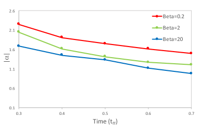
Figure 2.— Plot of $|\alpha|$ (y-axis) vs. $t$ (x-axis) for the range $0.3t_{ff}$ to $0.7t_{ff}$ where the power-law tail is well-developed.

Figure 3.— Plot of transition point $s_{t}$ (y-axis) versus time (x-axis) for each magnetic field strength as predicted by equation 9 (dashed lines) and those found through fitting (solid lines) and colors as in Figure 2.

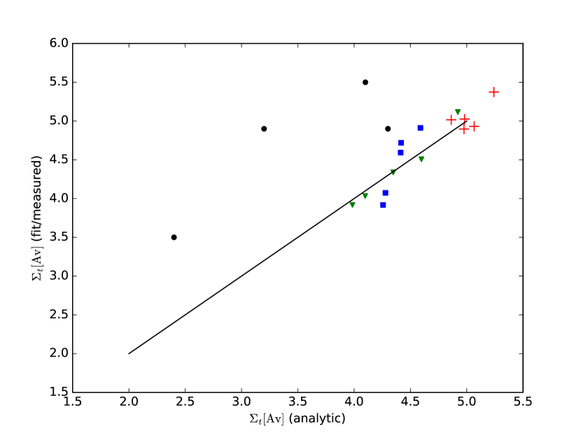
Figure 4.— Plot of fitted transition point vs analytic transition point for the three values of plasma $\beta$ along (colored points, blue square =$\beta=20$, green triangle=$\beta=2$, red +=$\beta=0.1$) with several observationally attained transition points (black circles) from nearby molecular clouds.

4. Observational Comparison

In this section we test our analytic prediction for the transitional column density against observations. In particular, Schneider et al. (2015, hereafter S15) published values of the mean column density $\Sigma_{0}$, transitional column density ($\Sigma_{t}$), the width of the lognormal ($\sigma_{s}$), and the slope of the power-law tail ($\alpha$) for four GMCs with different star formation histories and corrected for foreground and background dust contamination. This provides an observational test for comparing the predicted values of $\Sigma_{t}$ to the measured value, based on the measured values of $\Sigma_{0}$, $\alpha$ and $\sigma_{s}$ and the application of Equation 6. We list the LOS foreground/background corrected parameters as reported in S15 and the analytic predicted value for $\Sigma_{t}$ in Table 1.

Table 1Comparison of Measured and Predicted Transition Point. Simulated clouds are taken only at $t=0.5t_{\rm{ff}}.$

Cloud	$\Sigma_{0}$ (Av)	$\alpha$	$\sigma_{s}$	$\Sigma_{t,\rm{fit}}$ (Av)	$\Sigma_{t,\rm{an}}$ (Av),	reference
NGC3603	3.4	-1.31	0.52	4.9	4.3	S15
Carina	3.0	-2.66	0.38	5.5	4.1	S15
Maddalena	2.3	-3.69	0.32	4.9	3.2	S15
Auriga	1.6	-2.54	0.45	3.5	2.4	S15
$\beta=0.2$	3.4	$\approx$ -1.5	$\approx$ 0.5	4.9	5.1	this work
$\beta=2$	3.4	$\approx$ -1.5	$\approx$ 0.5	4.3	4.3	this work
$\beta=20$	3.4	$\approx$ -1.5	$\approx$ 0.5	4.6	4.4	this work

The values of $\Sigma_{t,S15}$ and $\Sigma_{t,Eq.\ref{eqn.st}}$ agree to within approximately $1.5\;A_{v}$, with predicted values being consistently smaller. We discuss the possible reasons for this in the next section.

5. Discussion

5.1. The HI-H₂ Transition and Self-Gravity

Recent studies have suggested that the PDF of molecular line tracers and dust tracers is of power-law form(Schneider et al., 2015; Lombardi et al., 2015) while the neutral diffuse HI builds up most of the lognormal portion of the PDF (Burkhart et al., 2015; Imara & Burkhart, 2016). In light of these recent studies, the HI lognormal PDF and H₂ power-law tail PDF may be effectively distinguished by the transition point between the two distributions. The truncation of the HI lognormal roughly corresponds to the HI-H₂ transitional column density in Galactic star-forming clouds(Burkhart et al., 2015; Imara & Burkhart, 2016) which suggests that measuring the transitional column density in such clouds could provide constraints on the HI-H₂ transition. The transitional column density is approximately $\Sigma_{t}=1-5\times 10^{21}\;{\rm cm}^{-2}$ (i.e. $\approx 8-38\;M_{\odot}/{\rm pc}^{2}$) which is in the range of the typically quoted HI-H2 transition value of approximately $10\;M_{\odot}/{\rm pc}^{2}$(McKee & Krumholz, 2010). An example of this is recent observations of the Perseus molecular cloud, which find a HI-H₂ transitional column density of $\Sigma=9-11\times 10^{21}\;{\rm cm}^{-2}$

5.2. Observational Properties of the Low Column Density PDF via $s_{t}$

Recently several authors (Schneider et al., 2015; Lombardi et al., 2015) have noted that dust emission and extinction are problematic probes of the low column density material in molecular clouds. This is because the observed PDF of dust can suffer several biases including resolution, noise, boundary effects and line-of-sight contamination. Lombardi et al. (2015) pointed out that while the lognormal portion of the PDF cannot be securely traced by dust, the characteristic break in the power-law regime at low values of extinction/column density (i.e. $s_{t}$) is still unaffected by observational biases.

These studies suggest that $s_{t}$ is a robust observational quantity, even though the properties of the lognormal PDF, such as the width of the lognormal, are not possible to accurately observe in dust tracers. Using our analytic expression for $s_{t}$ it is therefore possible to estimate the lognormal width of the distribution by measuring the power-law tail slope and value of s_t. The shape of the low-density portion of the PDF provides an important constraint on the initial conditions of star-forming clouds (i.e. the strength of turbulence and comparison to numerical studies) and therefore it is important to quantify this observationally.

Incidentally, the difficulty of constraining the width of the PDF may be the reason that our predicted value for $s_{t}$ differs by about $1.5\;A_{v}$ from the Herschel observations reported in Table 1 (Schneider et al. 2015), since our prediction depends on the width of the PDF. Since the measured values of $\alpha$ (slope of the power-law) and $s_{t}$ should be robust to observational effects, these two quantities should be used to measure the lognormal width $\sigma_{s}$, rather than fitting $\sigma_{s}$ directly from observations.

6. Conclusions

The transition point between the turbulence-dominated (lognormal) portion of the PDF and the denser, self-gravitating (power-law) portion of the PDF is an important component of the star-formation process. In this paper we derived an analytic expression for the transitional point ($s_{t}$) of the column density PDF from a lognormal to a power-law.

We find that:

• The expression for $s_{t}$ depends on the mean column density, width of the lognormal portion of the PDF (i.e. the sonic Mach number and driving parameter) and the slope of the power-law portion of the PDF (i.e. power-law index for a self-gravitating isothermal sphere)

• In the limit of strong collapse, $s_{t}$ represents the post-shock density given by the balance of turbulent and thermal pressure.

• The values predicted by the analytic expression for $s_{t}$ agree well with measurements from Herschel dust observations and Enzo AMR simulations.

• The analytic expression reported in Equation 6 will be useful for determining the properties of the PDF from unresolved low density material in observations and for estimating the HI-H₂ transition in clouds.

References

- Ballesteros-Paredes et al. (2011) Ballesteros-Paredes, J., Vázquez-Semadeni, E., Gazol, A., Hartmann, L. W., Heitsch, F., & Colín, P. 2011, MNRAS, 416, 1436
- Berkhuijsen & Fletcher (2008) Berkhuijsen, E. M. & Fletcher, A. 2008, MNRAS, 390, L19
- Bialy et al. (2015) Bialy, S., Sternberg, A., Lee, M.-Y., Le Petit, F., & Roueff, E. 2015, ApJ, 809, 122
- Burkhart et al. (2015) Burkhart, B., Collins, D. C., & Lazarian, A. 2015, ApJ, 808, 48
- Burkhart et al. (2009) Burkhart, B., Falceta-Gonçalves, D., Kowal, G., & Lazarian, A. 2009, ApJ, 693, 250
- Burkhart & Lazarian (2012) Burkhart, B. & Lazarian, A. 2012, ApJ, 755, L19
- Burkhart et al. (2013a) Burkhart, B., Lazarian, A., Ossenkopf, V., & Stutzki, J. 2013a, ApJ, 771, 123
- Burkhart et al. (2015) Burkhart, B., Lee, M.-Y., Murray, C. E., & Stanimirović, S. 2015, The Astrophysical Journal Letters, 811, L28
- Burkhart et al. (2013b) Burkhart, B., Ossenkopf, V., Lazarian, A., & Stutzki, J. 2013b, ApJ, 771, 122
- Burkhart et al. (2010) Burkhart, B., Stanimirović, S., Lazarian, A., & Kowal, G. 2010, ApJ, 708, 1204
- Collins et al. (2012) Collins, D. C., Kritsuk, A. G., Padoan, P., Li, H., Xu, H., Ustyugov, S. D., & Norman, M. L. 2012, ApJ, 750, 13
- Collins et al. (2011) Collins, D. C., Padoan, P., Norman, M. L., & Xu, H. 2011, ApJ, 731, 59
- Collins et al. (2010) Collins, D. C., Xu, H., Norman, M. L., Li, H., & Li, S. 2010, ApJS, 186, 308
- Elmegreen (2011) Elmegreen, B. G. 2011, ApJ, 731, 61
- Federrath & Klessen (2012) Federrath, C. & Klessen, R. S. 2012, ArXiv e-prints
- Federrath & Klessen (2013) —. 2013, ApJ, 763, 51
- Federrath et al. (2008) Federrath, C., Klessen, R. S., & Schmidt, W. 2008, ApJ, 688, L79
- Froebrich & Rowles (2010) Froebrich, D. & Rowles, J. 2010, MNRAS, 406, 1350
- Girichidis et al. (2014) Girichidis, P., Konstandin, L., Whitworth, A. P., & Klessen, R. S. 2014, ApJ, 781, 91
- Goodman et al. (2009) Goodman, A. A., Rosolowsky, E. W., Borkin, M. A., Foster, J. B., Halle, M., Kauffmann, J., & Pineda, J. E. 2009, Nature, 457, 63
- Hennebelle & Chabrier (2011) Hennebelle, P. & Chabrier, G. 2011, ApJ, 743, L29
- Hill et al. (2008) Hill, A. S., Benjamin, R. A., Kowal, G., Reynolds, R. J., Haffner, L. M., & Lazarian, A. 2008, ApJ, 686, 363
- Imara & Burkhart (2016) Imara, N. & Burkhart, B. 2016, ApJ, 771, 123
- Kainulainen et al. (2009) Kainulainen, J., Beuther, H., Henning, T., & Plume, R. 2009, A&A, 508, L35
- Kainulainen & Tan (2013) Kainulainen, J. & Tan, J. 2013, A&A, 549, 53
- Kritsuk et al. (2011) Kritsuk, A. G., Norman, M. L., & Wagner, R. 2011, ApJ, 727, L20
- Krumholz & McKee (2005) Krumholz, M. R. & McKee, C. F. 2005, ApJ, 630, 250
- Krumholz et al. (2009) Krumholz, M. R., McKee, C. F., & Tumlinson, J. 2009, ApJ, 693, 216
- Lee et al. (2012) Lee, M.-Y., Stanimirović, S., Douglas, K. A., Knee, L. B. G., Di Francesco, J., Gibson, S. J., Begum, A., Grcevich, J., Heiles, C., Korpela, E. J., Leroy, A. K., Peek, J. E. G., Pingel, N. M., Putman, M. E., & Saul, D. 2012, ApJ, 748, 75
- Li et al. (2015) Li, P. S., McKee, C. F., & Klein, R. I. 2015, MNRAS, 452, 2500
- Lombardi et al. (2015) Lombardi, M., Alves, J., & Lada, C. J. 2015, A&A, 576, L1
- McKee & Krumholz (2010) McKee, C. F. & Krumholz, M. R. 2010, ApJ, 709, 308
- McKee & Ostriker (2007) McKee, C. F. & Ostriker, E. C. 2007, ARA&A, 45, 565
- Molina et al. (2012) Molina, F. Z., Glover, S. C. O., Federrath, C., & Klessen, R. S. 2012, MNRAS, 423, 2680
- Padoan et al. (1997) Padoan, P., Jones, B. J. T., & Nordlund, A. P. 1997, ApJ, 474, 730
- Padoan & Nordlund (2011) Padoan, P. & Nordlund, Å. 2011, ApJ, 730, 40
- Price et al. (2011) Price, D. J., Federrath, C., & Brunt, C. 2011, in , 21
- Schneider et al. (2013) Schneider, N., André, P., Könyves, V., Bontemps, S., Motte, F., Federrath, C., Ward-Thompson, D., Arzoumanian, D., Benedettini, M., Bressert, E., Didelon, P., Di Francesco, J., Griffin, M., Hennemann, M., Hill, T., Palmeirim, P., Pezzuto, S., Peretto, N., Roy, A., Rygl, K. L. J., Spinoglio, L., & White, G. 2013, ApJ, 766, L17
- Schneider et al. (2014) Schneider, N., Ossenkopf, V., Csengeri, T., Klessen, R., Federrath, C., Tremblin, P., Girichidis, P., Bontemps, S., & Andre, P. 2014, ArXiv e-prints
- Schneider et al. (2015) Schneider, N., Ossenkopf, V., Csengeri, T., Klessen, R. S., Federrath, C., Tremblin, P., Girichidis, P., Bontemps, S., & André, P. 2015, A&A, 575, A79
- Shu (1977) Shu, F. H. 1977, ApJ, 214, 488
- Sternberg (1988) Sternberg, A. 1988, ApJ, 332, 400
- Vazquez-Semadeni (1994) Vazquez-Semadeni, E. 1994, ApJ, 423, 681
- Vazquez-Semadeni & Garcia (2001) Vazquez-Semadeni, E. & Garcia, E. 2001, ApJ, 557, 727