Provably unbounded memory advantage in stochastic simulation
using quantum mechanics.
Abstract
Simulating the stochastic evolution of real quantities on a digital computer requires a trade-off between the precision to which these quantities are approximated, and the memory required to store them. The statistical accuracy of the simulation is thus generally limited by the internal memory available to the simulator. Here, using tools from computational mechanics, we show that quantum processors with a fixed finite memory can simulate stochastic processes of real variables to arbitrarily high precision. This demonstrates a provable, unbounded memory advantage that a quantum simulator can exhibit over its best possible classical counterpart.
pacs:
03.67.-a, 02.50.Ey, 05.20.-yMany macroscopic processes we wish to simulate involve the dynamics of real numbers. The dynamical properties we wish to track (e.g. the position of an object) can take on almost any number, seemingly without noticeable quantization until one goes down to the Planck scale. The simulation of such processes necessitates compromise between the resources allocated and the precision with which we track such properties. Clever implementations to this problem, such as the floating point format IEE (2008), form the heart of modern computing technology – but all subscribe to the same trade-off: treating a quantity with higher precision requires the allocation of more memory. To perfectly replicate the future statistics of a continuous variable dynamical system exactly would inevitably require unbounded memory.
The advent of quantum technology, however, opens new possibilities. Not only has this technology shown great potential in solving problems many consider classically intractable Deutsch (1985); Deutsch and Jozsa (1992); Grover (1996); Shor (1997); Cleve et al. (1998), it has demonstrated the capability to greatly reduce the amount of information one needs to send in certain tasks requiring communication between distributed parties van Dam (2000); de Wolf (2001); Brassard . Could the memory required by a quantum machine that simulates dynamical processes likewise scale much more favourably with precision?
Here, we consider the simulation of a class of stochastic systems involving the dynamics of parameters that take on real numbers. Classical simulation of such processes digitally involves ‘coarse-graining’: the parameter at each point in time is approximated to bits of precision at some memory cost that scales linearly with . We construct quantum simulators the exhibit unbounded advantage. The quantum simulator can exactly replicate the statistics of a bit classical simulator for arbitrarily large using a bounded amount of memory. Thus, quantum simulators can side-step the precision-memory tradeoff – finite quantum memory can simulate such processes to arbitrary fixed precision.
This unbounded divergence has practical and foundational consequences. Practically, it suggests that quantum processors may be increasingly advantageous as we wish to simulate ever more memory-intensive systems, such as those arising from big data sets. Foundationally, the minimal memory required to simulate a process is a well-established measure of structure, known as statistical complexity Grassberger (1986); Crutchfield and Young (1989); Shalizi and Crutchfield (2001); Crutchfield et al. (2009); Crutchfield (2011); Haslinger et al. (2010); Shalizi et al. (2004); Marques da Silva et al. (1997); Clarke et al. (2003); Par (2007); Li et al. (2008); Lu and Brooks (2012). Our work suggests that there are certain processes which grow unboundedly in statistical complexity, but yet remain simple to an observer with quantum capabilities.
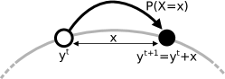
Cyclic random walks. Consider a small bead located on a circular ring of circumference 1 (as per figure 1). Its position can always be described by some real number . At each discrete time , the bead’s position is stochastically perturbed. This perturbation is described by a real random variable that is governed by a continuous probability density function , such that
| (1) |
where represents the random variable that governs the location of the bead at time , and denotes the fractional part of , such that positions differing only by whole rotations around the ring are equivalent. We refer to as the shift function, and assume the process is stationary, in the sense that has no explicit dependence on , and rotationally symmetric such that has no dependence on the current value of . This same formalism describes a diverse range of systems undergoing cyclic random walks, such as the azimuthal motion of gas molecules diffusing in an annular tube, or the position of a single electron travelling through an electric circuit with constant resistance.
We capture the dynamics of formally using the framework for describing stochastic processes. In general, a stochastic process is characterized by a bi-infinite sequence of random variables , that governs its value at each discrete time . For convenience, we often segregate past and future values, such that and respectively govern the values in the past and future with respect to time . The cyclic random walk above is then entirely captured by the joint probability distribution such that for any instance of the process with past values , future values will be observed with probability .
Here, we consider the simulations of the above process to ever increasing precision. We adopt a natural technique of discretizing a continuous process, by introducing a family of stochastic processes that describe discrete approximations of this process, where in each the position of bead is represented to bits of precision by a -digit binary number. This is done by limiting to a discrete set of equally–spaced values, (for to ). At each time-step, the probability that a bead in discrete location transitions to , is given by the probability that a bead initially at will transition to any value of whose bit binary representation is . That is
| (2) |
where represents the interval on the ring that is ‘rounded to’ . This results in a Markovian stochastic process that emits a symbol from the finite alphabet at each time-step, whose dynamics are governed by the stochastic matrix with elements . As , the statistics of approach that of ; at the potential cost of tracking more information111An alternative discretization is to calculate the transition probabilities by assuming the initial value of is uniformly distributed in . This yields asymptotically identical statistics as , and does not change the results of this article..
Classical simulation costs scale with precision. We can formally describe simulators using the tools of computational mechanics Crutchfield and Young (1989); Shalizi and Crutchfield (2001); Crutchfield et al. (2009); Crutchfield (2011). A simulator of a process is a device whose future output behaviour conditioned on any particular past should be statistically indistinguishable to the process itself. Specifically, let the state of the simulator at each time be , such that at the subsequent time-step it can output and transition to state . For this device to be a statistically faithful simulator of a process , we require that:
-
1.
For each specific past at each time , we can deterministically configure the device using a function into some state , such that it will produce future outputs with probability .
-
2.
If a simulator is in state at time , and outputs in the subsequent time-step, its internal state must then transition to .
The first condition ensures the simulator can be initialized to simulate desired conditional future statistics; the second that a correctly initialized simulator continues to exhibit statistically correct statistics at every time-step. The memory cost of the simulator corresponds to the storage requirements of this internal state. This cost is bounded from below by the information entropy of the random variable . In the asymptotic limit of many independent identically distributed copies of the simulator, this bound is tight as the ensemble of states may be compressed (such as by Shannon’s noiseless encoding theorem Shannon (1948), or Schumacher compression Schumacher (1995); Winter (1999)). Physically a simulator can be viewed as a communication channel in time: it represents the exact object Alice must give to Bob at each time-step that captures sufficient past information for Bob to replicate the processes conditional future behaviour. is known as the encoding function, which describes how the past is encoded within the channel.
This memory cost of the provably-optimal classical simulator – known as the statistical complexity – is extensively studied in complexity science Crutchfield and Young (1989). This value captures the absolute minimum memory any classical simulator of a process must store, and thus is a prominent quantifier of a process’s structure and complexity222 The statistical complexity is distinct from algorithmic information (Kolmogorov–Chaitin complexity). Statistical complexity is, as the name would imply, intrinsically statistical – concerned with the replication of the statistical behaviour of a process; whereas algorithmic information relates to the compressibility of an exact string Ladyman (2013). (e.g. Crutchfield (2011); Marques da Silva et al. (1997); Clarke et al. (2003); Shalizi et al. (2004); Par (2007); Li et al. (2008); Haslinger et al. (2010); Lu and Brooks (2012)). Such an optimal simulator can be explicitly constructed, and corresponds to the simulator that stores in its internal memory the causal states of the process Crutchfield and Young (1989); Shalizi and Crutchfield (2001): defined by an encoding function such that if and only if (i.e. the conditional futures of and coincide).
In our cyclic random walks, each is a first-order Markov process: the statistics of future outcomes depend only on the most recent value of . When this example is discretized, the causal states are thus typically in one-to-one correspondence with the discrete values that can take333There are exceptions, such as when for , and the system jumps to a completely random point at each time-step; here there is only one causal state for all , because the current position no longer affects the future outcomes at all.. That is, has causal states, labelled , where corresponds to the set of pasts ending in . When the simulator has been running for a sufficiently long time, the probability distribution over the internal memory converges on for each – its steady state, in which all causal states occur with equiprobability. Thus, the classical statistical complexity
| (3) |
scales linearly with the precision.
Quantum simulators are memory–efficient. It has recently been shown that quantum processors have the capability to simulate stochastic processes with less memory than is classically possible Gu et al. (2012); Suen et al. (2015); Mahoney et al. (2016); Palsson et al. (2016); Riechers et al. (2016). Here, we construct an explicit quantum simulator for the cyclic random walk. Instead of storing each causal state directly, our quantum simulator stores a corresponding quantum state
| (4) |
where forms an orthonormal basis.
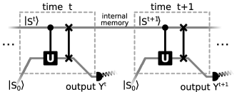
The stationary state of the quantum simulator is then given by the quantum ensemble state (as all quantum states occur with equiprobability). Thus the memory required to store these states is given by the von Neumann entropy given , where are the eigenvalues of . The key improvement here is that are not in general mutually orthogonal, and thus is generally less than . Nevertheless a quantum circuit (outlined in figure 2 – with details in the Technical Appendix) acting on these quantum states will produce statistically identical outputs to the classical simulator.
The von Neumann entropy of a quantum state is equal to the Shannon entropy of the outcome statistics of a projective measurement on that state, minimized over all choices of projective measurement. This minimization corresponds to a measurement in the basis in which the state’s density matrix is diagonal. A classical probability distribution maps onto a mixed quantum state, diagonal in a fixed basis. As such, the stationary state of the classical simulator can be assigned a quantum state, whose von Neumann entropy is exactly that distribution’s Shannon entropy. This allows us to compare the entropic cost of the classical and quantum machines’ memories on an equal footing.
Unbounded advantage of quantum memory. We now come to the main claim of our paper: there are stochastic processes that can be simulated to infinite precision using a finite amount of quantum memory.
Explicitly, we show that for certain cyclic processes, the quantum ensemble state’s eigenvalues satisfy for some finite value . Our result relies on first observing that the eigenvalues can be directly related to transition probabilities via the relation
| (5) |
where denotes the discrete Fourier transform, . (The proof relies on invoking the cyclic symmetry of the process – and hence of the transition probabilities – and is explicitly derived in the Technical Appendix). The spread (as a function of ) is an indicator of how quickly a particle diffuses in the random walk. Thus, the Fourier-like relation between and indicates an inverse relationship between the amount of diffusion in the cyclic process and the spread of eigenvalues. The greater the variance of , the more quickly a particle diffuses, and the smaller the spread of – resulting in a reduced quantum memory requirement. We now show that for some natural examples, this reduction is sufficiently large that remains bounded for all (as illustrated in figure 3).
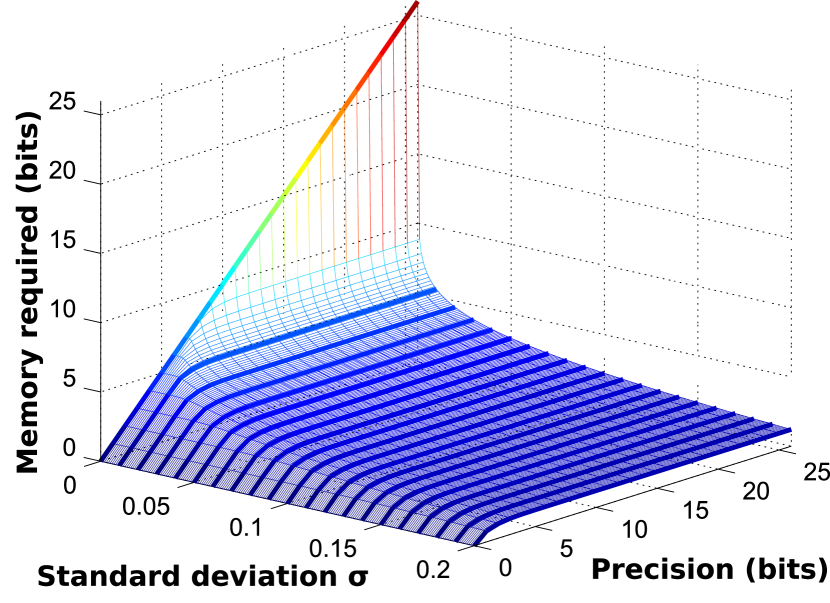
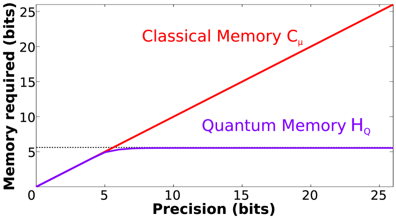
Example 1: Gaussian noise. A cyclic process rotating at a constant rate subject to Gaussian noise has a shift function given by a Gaussian distribution about mean with standard deviation . Here, characterises the average velocity (in terms of the variable’s mean displacement per time-step), and the size of the fluctuations. When , this process corresponds to Gaussian diffusion. For our analysis, we take and thus ignore fluctuations where the particle travels more than a complete loop around the ring in a single time-step (a value of ensures that such events are less likely than one part in a million.)
As can be seen in figures 3(a) and 3(c), as the desired precision increases, the memory cost of simulating this process quickly converges onto a constant determined by the fluctuation strength ; ultimately, infinite-precision simulation is possible using only a finite quantum memory. This behaviour may be understood analytically by seeing that for large , the eigenvalues associated with the quantum simulator’s internal memory are also given by samples from a Gaussian distribution: for , where for convenience we have cyclicly offset the label of the eigenvalues’ indices by (proof in Technical Appendix). This demonstrates that increasing tightens the spread of eigenvalues, and thus reduces the memory requirement for the quantum simulator.
In the Technical Appendix, we prove that as the precision increases, the sum converges on a finite value, bounded (in bits) by
| (6) |
Thus, for any fixed , the Gaussian random walk may be simulated to arbitrarily high precision using a quantum simulator of bounded entropy. Moreover, this also implies an unbounded divergence between the classical and the quantum statistical complexity Suen et al. (2015); Aghamohammadi et al. (2016) , which is upper bounded by .
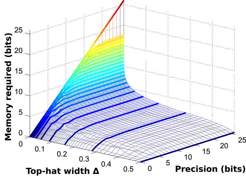
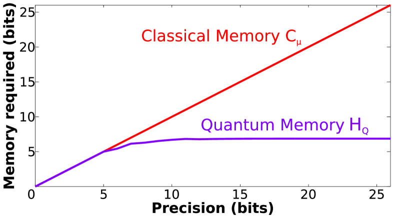
Example 2: Uniform white noise. In the second example, we consider a particle that is perturbed by uniformly distributed noise. At each time-step, the particle can move anywhere in the range of from its current position with uniform probability, where . Again, characterises the average velocity, and here the size of the fluctuations. The associated shift function is a top-hat function, that has a uniform value of in the range and everywhere else.
The entropy of the quantum simulator, is plotted for various precision in figures 3(b) and 3(d). We see that for any fixed , the quantum memory required by our simulator converges to a bounded value. As in the Gaussian scenario, the quantum simulator can replicate a classical simulation to any given precision using with finite entropy. In the Technical Appendix, we prove this analytically. We show that as , the entropy remains finite, and is bounded above by . In particular, for large , the eigenvalues of the relevant ensemble state obey for , where is the normalized sinc function, . Larger values will result in a smaller spread of eigenvalues, and result is smaller . For any given the entropy is finite in the limit . This establishes a second natural example where the quantum simulator can demonstrate an unbounded memory advantage over its best possible classical counterpart.
The origin of quantum advantage. The source of classical inefficiency can be understood by considering dynamics on causal states. Consider two instances of , one where , and the other where . As their conditional future statistics differ [that is, ], a classical simulator must be configured differently for each instance (corresponding to being initialized in one of two different causal states, or ). Nevertheless, there is finite probability that at the next time-step, both instances of the process emit the same output (up to precision ). Should this happen, we would not be able to use the current state of the machine to determine the causal state it was in at the previous time. That is, there is some probability that the distinction between and will never be reflected in the future statistics of the process – a phenomenon known as crypticity Mahoney et al. (2009, 2016). As increases, this occurs with greater likelihood (tending to unit probability as ), and thus proportionally more information is wasted. Ultimately, in the limit of high precision, a vanishingly small proportion of the information stored in the classical memory is pertinent to the statistical behaviour of the process’s future.
Quantum simulators compensate for this waste by mapping these causal states to non-orthogonal quantum states. The quantum state (eq. 4) associated with neighbouring causal states ( and ) also become increasingly similar with increasing – resulting in progressively greater savings. Consider the Gaussian scenerio, where is bounded by equation (6). For small , the memory cost scales as , such that halving the variance of fluctuations at each time-step adds one bit to the memory cost of the quantum simulator. The standard deviation of the shift function has set an effective length scale over which the system must be simulated classically. The statistical behaviour of future outputs from two systems that are initially prepared in points separated by more than one standard deviation are typically distinguishable, and so these points must be stored as nearly-orthogonal quantum states at some memory cost. On the other hand, when two points are initially closer than the standard deviation scale, the probability that they could be distinguished by their future behaviour diminishes, and they may be represented by increasingly overlapping quantum states. In this regime, a fixed finite memory can accommodate any desired precision.
We gain further insight into the origins of quantum advantage by considering the cases where it does not appear: and . In both these cases, the shift function is a Dirac delta distribution. As such, no matter how high the precision, by observing the future outputs, it will always be possible to distinguish whether the system came from some site or its neighbour ; the dynamics of the system are wholly reversible. If always transitions to and always to , being able to distinguish between these two sites is crucial to produce the correct statistical behaviour, even as the precision increases. As such, the quantum simulator cannot tolerate overlap between the states and , and must store them orthogonally (allowing them to be distinguished). In this scenario, the quantum simulator cannot demonstrate any advantage in memory cost over its classical analogue.
Discussion and outlook. In this article, we presented a task in which quantum mechanics has an unbounded memory advantage over the most memory-efficient classical alternative: the simulation of a classical cyclic stochastic process. We found that the classical simulator has a memory requirement that scales linearly with the precision required, while the quantum simulator’s requirement may be bounded by a finite value, even at arbitrarily-high fixed precision. This establishes a rare scenario where the scaling advantage of quantum processing can be provably established.
This finding leads to a number of natural open questions – the first being of generality. Certainly, the examples presented are sufficiently simple that such divergences are unlikely to be merely a mathematical oddity. The unbounded quantum advantage relies on having two properties: (a) the number of causal states grows with , and (b) the conditional future statistics between different causal states converges sufficient quickly with . If these conditions can be formalized, we may be able to establish similar divergences in much more general scenarios, such as the simulation of non-Markovian or non-cyclic processes. Beyond von Neumann entropy, it would be interesting if similar scaling can be found for other metrics of memory cost, such as the dimension – namely, whether there is an encoding that allows for simulation to arbitrary precision using a Hilbert space of bounded dimension. Meanwhile the inefficiency of classical simulators have show to directly results in unavoidable increased heat dissipation Wiesner et al. (2012); Still et al. (2012); Garner et al. (2015). This hints that quantum processing may allow significant energetic savings for stochastic simulation, especially for systems that become increasingly difficult to simulate as they scale in size.
On a foundational level, the statistical complexity is often regarded as a fundamental measure of a process’s intrinsic structure – the rationale being that it quantifies the minimal amount of information about a process’s history that must be recorded to allow for predictions about that process’s future behaviour. The measure has been applied to understand structure within diverse complex settings: from the dynamics of neurons Haslinger et al. (2010) and the stock market Par (2007), to quantifying self-organization Shalizi et al. (2004), among other examples Marques da Silva et al. (1997); Clarke et al. (2003); Li et al. (2008); Lu and Brooks (2012). The discovery of more efficient quantum models has led to the idea that the complexity of a system depends on what sort of information we use to observe it Suen et al. (2015); Aghamohammadi et al. (2016). In this context, our results establish a family of processes that can look ever more complex classically, but remain simple quantum-mechanically. It would fascinating to see if divergences between quantum and classical complexities can be found in existing studies, such as the examples above. Could it be that these systems appear complex classically – but look much simpler when viewed through the lens of quantum theory?
ACKNOWLEDGEMENTS
We thank James Crutchfield, Thomas Elliott, David Garner, Peter Grassberger, Jan-Åke Larsson, and Chengran Yang for helpful comments and discussions. We gratefully acknowledge funding from the John Templeton Foundation Grant 53914 “Occam’s Quantum Mechanical Razor: Can Quantum theory admit the Simplest Understanding of Reality?”; the Foundational Questions Institute; the Ministry of Education in Singapore, the Academic Research Fund Tier 3 MOE2012-T3-1-009; and the the National Research Foundation of Singapore (Award Nos. NRF–NRFF2016–02 and NRF–CRP14-2014-02).
TECHNICAL APPENDIX
Classical costs from computational mechanics. We here present some minimal details from the mathematical framework of computational mechanics Crutchfield and Young (1989); Shalizi and Crutchfield (2001); Crutchfield et al. (2009); Crutchfield (2011) to substantiate the claim that the classical simulator’s minimal memory cost is equal to the precision .
In computational mechanics, the evolution of a dynamical property (over domain ) is characterised by a discrete-time stochastic process , written as bi-infinite sequence of random variables , where each random variable governs the value of the dynamical property at time . The statistical behaviour of a process may be represented in a causal manner by writing it as the conditional probability distribution , where is the infinite string of random variables occuring after time , and is the infinite string of random variables occuring before (and including) time . For stationary processes (such as the time-independent cyclic random walks described in this article), this distribution has no explicit time dependence, so we omit the superscript .
A faithful simulator of process is a machine (or program) that, having been initialized in accordance with the observation of past , then generates a series of outputs according to the distribution . Since storing an infinite string may require an unbounded amount of memory, one instead configures the internal state of the simulator (over configuration space ) according to some function , satisfying , where is the random variable describing the internal state of the simulator (formed by applying the function on each variate of ). Moreover, once initiated into state , when the simulator outputs in the subsequent time-step, its internal state must then transition to the state (where indicates the concatenation of to the end of string ).
The memory cost of such a simulator is given by the information entropy of , . The function that minimizes this classically corresponds to identifying the causal state of a particular past Crutchfield and Young (1989); Shalizi and Crutchfield (2001), defined by the equivalence relationship: for pasts and if and only if for all possible future values . The causal states are unique for any given process, and so their entropy is a property of the process itself known as its statistical complexity , capturing the intuition that a more complex process requires more memory to simulate.
For Markovian processes, such as discussed in this article, the number of causal states required is equal to the number of unique rows in the stochastic matrix describing the evolution. When these rows are generated by the discretization of a continuous process into divisions – such as when they are derived from the cyclic walk’s shift function – the number of states will be equal to , except for very specific (e.g. pathologically fractal) choices of and . Since by symmetry the probability of the simulator being in any particular state is equal, the classical memory cost of a simulator hence scales with the number of sites as , or linearly with the precision .
Details of the quantum circuit in figure 2. Let us consider figure 2 in more depth (see also Gu et al. (2012)). The circuit consists of one persistent internal memory state, and an “output tape”—a line of quantum states, which are fed into the system one at a time. Suppose each state on the output tape is initialized into some arbitrary state . For any two quantum states and in the same Hilbert space, it is always possible to construct a unitary transformation such that . This will be of the form where are states orthogonal to each other and to , and are states orthogonal to each other and to . Thus, in the joint Hilbert space of two quantum systems of dimension , it is possible to build a “controlled” unitary operation containing the elements for every in an arbitrary (generally non-orthogonal) set of states . [Note: the orthogonality of allows us to pairwise use the above construction for each .]
For a Markovian process discretized such that the stochastic matrix with elements describes its evolution, the above prescription supplies the unitary operation required for our quantum simulator when we set each , as per eq. 4 (states and are in the same basis).
We may now evaluate the action of a single time-step (grey dashed box within figure 2). Here, the joint Hilbert space corresponds to that of the internal memory together with the output tape. In the figure, we explicitly wrote the initial state of the output tape as , but this is arbitrary; any could be made into by acting on it first with a unitary gate containing . At the start of a time step, the internal memory is in state . Hence, the joint state of the memory and output tape is initially . After the controlled unitary is applied, the memory and tape will be in the entangled state . Applying a coherent swap operation (i.e. exchanging the labels of the Hilbert spaces) will take this joint state to – the state of the system at the end of the grey box.
The tape system is then ejected from the simulator. If one were to measure this state in the basis, one projects onto state with probability , and hence the output statistics of this measurement match that of the process being simulated. Moreover, after measuring, due to the entanglement, we know that when is measured, the internal memory must be in state , which is exactly the quantum state that would have been prepared if we had mapping the output statistics onto a classical causal state and then prepared directly. Hence, the quantum circuit in figure 2 can function as a discretized simulator for a Markovian process.
However, it is very important to note that there is no need whatsoever to measure the output tape for the quantum simulator to continue functioning. If it suits one’s purpose to store the output states in quantum memory (e.g. to perform further quantum information processing on the output data), then the quantum simulator still functions correctly. In this mode of operation, the measurements can be omitted from figure 2, and after steps, the simulator would have produced the entangled state
| (7) |
where is the quantum state that would have been prepared if the system was originally in causal state then outputted string , and a new causal state directly set according to this output sequence. Measuring the string of output tape subsystems thus still ensures that the internal memory state collapses into the correct causal state , conditional on the string observed.
In the first mode of operation (as drawn in figure 2), only one ancillary quantum system is required, as it can be reset and re-used between timesteps (the output tape carries away classical information only). In the second mode, the quantum output explicitly fulfils the role of the ancillary system, and a fresh ancillary system (provided by the “blank” output tape set to some fixed choice of pure quantum state) is inserted at each time step. In both modes, the ancillary system does not need to persist between time steps in order for the simulator to continue producing statistically correct outputs. As such, in both cases, it is the von Neumann entropy of the first subsystem, which remains within the simulator at all times, that we consider to be the internal memory cost.
Derivation of discrete eigenspectrum. The quantum machine state corresponding to the system being in classical state is given as . Assuming is simply connected, the quantum machine will reach a stationary state . Rather than directly calculating the entropy of , we can instead evaluate the entropy of the associated Gram matrix , whose elements are given by the overlaps .444 This works by constructing a fictitious purification of , given (where is an orthonormal basis) such that and . Since the von Neumann entropy of pure state is , it follows from triangle inequalities that . The circular symmetry of the cyclic random walk ensures that the discretized transition probabilities satisfy (that is, the transition probabilities depend only on differences between indices). It hence follows that the Gram matrix associated with is circulant Gray (2005). Since all rows can be derived by cyclic permutation of the top row, we shall drop one index and write the top row as . The eigenvalues of the Gram matrix are given by for , which can immediately be recognized as the discrete Fourier transform (DFT) of , which we denote as .
Moreover, the inner product , has the form of a convolution , where we have rewritten as such that is the -periodic extension of the reflection of ; and . We may then apply the circular convolution theorem to find the eigenvalues of , and therefore of :
| (8) |
These eigenvalues can hence be found efficiently by numerical algorithms, such as the fast-Fourier transform.
Example: Dirac-delta shift function. Let the shift function be for some . It can be seen that all except for the one at index that incorporates the delta peak where . Hence, and , and so for all . Thus, the von Neumann entropy of the simulator’s memory is .
Example: Uniform shift function. Consider the uniform shift function for . Here, , and so for and for all other . As such, we find that the eigenvalue , and all other eigenvalues , and hence the entropy of the Gram matrix is zero, for all values of .
Sampling Fourier transforms. It will be useful to show an auxiliary relationship between discrete and continuous Fourier transforms. Let be a function over the range that is sampled at equally spaced points with values given by for . We can construct a function , whose Fourier transform is
| (9) |
which when evaluated at integer is exactly the DFT of the samples , which we write as .
If is periodic, it is always possible to offset the position of the sample window of by some integer without changing the values of ’s DFT. For the functions we consider in this article, it is more convenient to start at , since typically and . Moreover, once the sample window has been set, the values of outside this window can not affect , since they do not feature in the sum. Thus, instead of considering sampling across a finite window, we can consider an infinite delta train sampled at the same intervals, but across a function where inside the range of the sample window (i.e. for the window used in this article) and outside this range. Here
| (10) |
where we have used the convolution theorem in the final step. The periodic sampling of causes the Fourier transform to be periodic with period (a phenomenon known as aliasing), such that ; the convolution with a delta train effectively makes a periodic sum of . This periodicity allows us the freedom to choose a convenient range of . In this article, we will typically use to . If outside the chosen range, then we can approximate
| (11) |
Asymptotic limit of eigenvalues. For large , we can derive an expression for in terms of the probability density function . We substitute with , which for Riemann-integrable is an arbitrarily good approximation in the limit of . Similarly, we may substitute with , where denotes the -periodic extension555Equivalent to wrapping to before evaluating . of . Taking the limit of the Riemann sum for a product of two functions, we then see
| (12) |
where . Moreover, since only has support in , we can rewrite the integral limits from to , and conclude that sampled at . Thus by treating as samples from a function at discrete intervals of , we find that for large , and hence
| (13) |
As shown in eq. (10), the eigenvalues are given by evaluated at integers , where over an (arbitrary) single period of and takes the value zero elsewhere. Due to the periodic summation, it can be seen also that , and so we are also free to choose the most convenient range for , which will typically be from to . If when , then the approximation
| (14) |
is reasonable. This assumption amounts taking enough samples of to admit a faithful reconstruction of under the Nyquist–Shannon theorem Shannon (1949). This holds true for the examples we shall now consider, where we will ultimately take large values of .
Example 1: Gaussian noise. Suppose the shift function of the particle is given by a Gaussian distribution about with standard deviation such that we can ignore the probability of the particle looping around the ring.
Derivation of eigenvalues. We can express as a Gaussian:
| (15) |
It can be easily verified that .
We also note that is also Gaussian:
| (16) |
Likewise, we can express as a Gaussian:
| (17) |
Taken together (making sure to substitute in the correctly modified values of and ), this allows us to provide an analytic solution for eq. (14) for Gaussian shift functions:
| (18) |
Hence, we see that choosing Gaussian transfer function with standard deviation corresponds to a spectrum of eigenvalues with standard deviation .
Upper bound on quantum memory cost. We now demonstrate that the entropy of such a system, given , is finite by bounding it from above. For convenience, we write where and , and will perform the calculation in units of nats. Thus, consider , explicitly
| (19) |
By setting , we find that has stationary points at , and when
| (20) |
When , these last two solutions disappear, and since we are in the regime of , this condition is satisfied. Hence, for small , monotonically decreases from its maximum value at for both positive and negative . This allows us to apply the Maclaurin–Cauchy integral bound (see e.g. Knopp (1990)),
| (21) |
which holds for any monotonically decreasing region of a function (here, ).
Using known results for definite Gaussian integrals,
| (22) |
we evaluate
| (23) |
Since , we find from equation (20) that
| (24) |
To obtain a bound on , we double the above since is even, and multiply by to convert from nats to bits (equivalently, change the base to since ): . In terms of the shift function’s standard deviation , this gives our result
| (25) |
In the limit of small , the leading term of the entropy thus scales with , such that halving the width of the standard deviation adds one bit to the maximum required quantum memory cost.
Example 2: Uniform white noise. The normalized top-hat (rectangular) shift function allowing for jumps of up to around a constant displacement is written
| (26) |
Derivation of eigenvalues. Taking the square root of this function alters its normalization, but not its shape: .
Suppose . In this case, yields the triangle function
| (27) |
This function is independent of the constant displacement . Indeed, non-zero only results in perfectly cancelling terms and in the Fourier transform.
Basic Fourier analysis tells us that transforms into a normalized sinc function (), and the triangle function into the square of this: . As this tends to for large , we can approximate the values of for large using eq. (14), to find the eigenspectrum
| (28) |
Upper bound on quantum memory cost. Through the careful deployment of mildly intimidating algebra, we can also derive an upper bound on entropy cost of simulating the square shift function. The outline of the proof is as follows. To bound where , we first construct a monotonically decreasing function that satisfies at every , and then show that is bounded from above. This sum will hence also upper-bound . As with the Gaussian example, for algebraic convenience, we will use natural logarithms and only consider the region of positive . In the final stage, we will convert from nats to bits, and use the evenness of to arrive at the full bound.
Explictly, we write
| (29) |
where we have made the substitution .
In the region , we can expand
| (30) |
The function has a maximum value of at , and so we can upper bound by making the substitution of with . Since , in the region where , we can likewise upper bound by making the substitution of with . Thus, for the region , we have a function given
| (31) |
However, as we plan to ultimately apply the Maclaurin–Cauchy integral convergence test, it is only convenient to use this upper bound in the region of where monotonically decreases. We identify this region by setting , to find that decreases monotonically when , descending from its maximum value of .
However, once again consider . Since it has the form of , it follows that in any region, . Since , we can then upper bound in the region of to form the monotonically decreasing function given
| (32) |
that is guaranteed to satisfy for all . At this point, it is convenient to express this again in terms of , making the substitution :
| (33) |
where represents the lowest integer above (or including) . This rounding is necessary since is in general not an integer. To upper bound at all points, we must round up this split between the regions of , since upper bounds all . (I.e. being slightly too inclusive in the first region will result in a slightly higher value of for the first satisfying ).
Having derived our monotonically decreasing function , we are now in a position to show that is finite for . Writing (for an upper bound, it is fine if a term is counted twice!), we evaluate the two regions separately. Firstly,
| (34) |
where we have used . Secondly, using the Maclaurin-Cauchy integral test (see e.g. Knopp (1990)), we bound
| (35) |
where the second line follows by substituting with the maximum value of , and by failing to round up the lower bound of the integral (thus including an extra contribution equal to ). This integral may be analytically solved,
| (36) |
Combining these two terms, we arive at:
| (37) |
Finally, to bound the entropy , we must double the above ( is even, and equation (37) bounds only the region ), and we convert from nats to bits (by including a factor of ):
| (38) |
By evaluating the constant terms, approximately,
| (39) |
yielding our result.
References
- IEE (2008) IEEE. IEEE Standard for Floating-Point Arithmetic. IEEE Std 754-2008, Aug 2008. doi: 10.1109/IEEESTD.2008.4610935.
- Deutsch (1985) D. Deutsch. Quantum Theory, the Church-Turing Principle and the Universal Quantum Computer. Proceedings of the Royal Society A: Mathematical, Physical and Engineering Sciences, 400(1818):97–117, jul 1985. ISSN 1364-5021. doi: 10.1098/rspa.1985.0070.
- Deutsch and Jozsa (1992) D. Deutsch and R. Jozsa. Rapid Solution of Problems by Quantum Computation. Proc. R. Soc. Lond. A., 439(1907):553–558, 1992. ISSN 09628444. URL http://www.jstor.org/stable/52182.
- Grover (1996) L. K. Grover. A fast quantum mechanical algorithm for database search. In Proceedings of the twenty-eighth annual ACM symposium on Theory of computing, STOC ’96, pages 212–219, New York, NY, USA, 1996. ACM. ISBN 0-89791-785-5. doi: 10.1145/237814.237866.
- Shor (1997) P. W. Shor. Polynomial-Time Algorithms for Prime Factorization and Discrete Logarithms on a Quantum Computer. SIAM J. Comput., 26(5):1484–1509, oct 1997. ISSN 0097-5397. doi: 10.1137/S0097539795293172.
- Cleve et al. (1998) R. Cleve, A. K. Ekert, C. Macchiavello, and M. Mosca. Quantum algorithms revisited. Proc. R. Soc. Lond. A., 454(1969):339–354, Jan 1998. doi: 10.1098/rspa.1998.0164.
- van Dam (2000) W. van Dam. Nonlocality & Communication Complexity. PhD thesis, University of Oxford, 2000.
- de Wolf (2001) R. M. de Wolf. Quantum Computing and Communication Complexity. PhD thesis, University of Amsterdam, 2001. URL http://dare.uva.nl/record/1/194123.
- (9) Gilles Brassard. Quantum Communication Complexity. Foundations of Physics, 33(11):1593–1616. ISSN 1572-9516. doi: 10.1023/A:1026009100467.
- Grassberger (1986) P. Grassberger Toward a quantitative theory of self-generated complexity International Journal of Theoretical Physics, 25:(9):907–938, 1986 ISSN 0020-7748 doi: 10.1007/BF00668821
- Crutchfield and Young (1989) J. P. Crutchfield and K. Young. Inferring statistical complexity. Physical Review Letters, 63:(2):105–108, 1989. ISSN 00319007. doi: 10.1103/PhysRevLett.63.105.
- Shalizi and Crutchfield (2001) C. R. Shalizi and J. P. Crutchfield. Computational mechanics: Pattern and prediction, structure and simplicity. Journal of Statistical Physics, 104(3-4):817–879, 2001. ISSN 00224715. doi: 10.1023/A:1010388907793.
- Crutchfield et al. (2009) J. P. Crutchfield, C. J. Ellison, and J. R. Mahoney. Time’s barbed arrow: Irreversibility, Crypticity, and stored information. Physical Review Letters, 103(9):094101, 2009. ISSN 00319007. doi: 10.1103/PhysRevLett.103.094101.
- Crutchfield (2011) J. P. Crutchfield. Between order and chaos. Nature Physics, 8(1):17–24, dec 2011. ISSN 1745-2473. doi: 10.1038/nphys2190.
- Haslinger et al. (2010) R. Haslinger, K. L. Klinkner, and C. R. Shalizi. The computational structure of spike trains. Neural computation, 22(1):121–57, jan 2010. ISSN 1530-888X. doi: 10.1162/neco.2009.12-07-678.
- Shalizi et al. (2004) C. R. Shalizi, K. L. Shalizi, and R. Haslinger. Quantifying self-organization with optimal predictors. Physical review letters, 93(11):118701, sep 2004. ISSN 0031-9007. doi: 10.1103/PhysRevLett.93.118701.
- Marques da Silva et al. (1997) J.G. Marques da Silva, J.C. Sartorelli, W.M. Gonçalves, and R.D. Pinto. A scale law in a dripping faucet. Physics Letters A, 226(5):269–274, feb 1997. ISSN 03759601. doi: 10.1016/S0375-9601(96)00941-3.
- Clarke et al. (2003) R. W. Clarke, M. P. Freeman, and N. W. Watkins. Application of computational mechanics to the analysis of natural data: An example in geomagnetism. Physical Review E, 67(1):016203, jan 2003. ISSN 1063-651X. doi: 10.1103/PhysRevE.67.016203.
- Par (2007) J. B. Park, J. W. Lee, J.-S. Yang, H.-H. Jo, and H.-T. Moon. Complexity analysis of the stock market. Physica A: Statistical Mechanics and its Applications, 379(1):179–187, jun 2007. ISSN 03784371. doi: 10.1016/j.physa.2006.12.042.
- Li et al. (2008) C.-B. Li, H. Yang, and T. Komatsuzaki. Multiscale complex network of protein conformational fluctuations in single-molecule time series. Proceedings of the National Academy of Sciences of the United States of America, 105(2):536–41, jan 2008. ISSN 1091-6490. doi: 10.1073/pnas.0707378105.
- Lu and Brooks (2012) C. Lu and R. R. Brooks. P2P hierarchical botnet traffic detection using hidden Markov models. In Proceedings of the 2012 Workshop on Learning from Authoritative Security Experiment Results - LASER ’12, pages 41–46, New York, New York, USA, jul 2012. ACM Press. ISBN 9781450311953. doi: 10.1145/2379616.2379622.
- Shannon (1948) C. E. Shannon. A mathematical theory of communication. Bell Sys. Tech. Jour., 27(3):379–423,623–656, Jul 1948. ISSN 00058580. doi: 10.1002/j.1538-7305.1948.tb01338.x.
- Schumacher (1995) Benjamin Schumacher. Quantum coding. Physical Review A, 51(4):2738–2747, Apr 1995. ISSN 1050-2947. doi: 10.1103/PhysRevA.51.2738.
- Winter (1999) Andreas Winter. Coding Theorems of Quantum Information Theory. PhD thesis, Universit’́at Bielefeld, Apr 1999. URL http://arxiv.org/abs/quant-ph/9907077.
- Ladyman (2013) J. Ladyman, J. Lambert, and K. Wiesner. What is a complex system? European Journal for Philosophy of Science 3 33-67, 2013 doi: 10.1007/s13194-012-0056-8
- Gu et al. (2012) M. Gu, K. Wiesner, E. Rieper, and V. Vedral. Quantum mechanics can reduce the complexity of classical models. Nature Communications, 3:762, 2012. ISSN 2041-1723. doi: 10.1038/ncomms1761.
- Suen et al. (2015) W. Y. Suen, J. Thompson, A. J. P. Garner, V. Vedral, and M. Gu. The classical-quantum divergence of complexity in the Ising spin chain. Quantum 1:25, 2017. doi: 10.22331/q-2017-08-11-25
- Mahoney et al. (2016) J. R. Mahoney, C. Aghamohammadi, and J. P. Crutchfield. Occam’s Quantum Strop: Synchronizing and Compressing Classical Cryptic Processes via a Quantum Channel. Scientific reports, 6:20495, Jan 2016. ISSN 2045-2322. doi: 10.1038/srep20495.
- Palsson et al. (2016) M. S. Palsson, M. Gu, J. Ho, H. M. Wiseman, and G. J. Pryde. Experimentally modeling stochastic processes with less memory by the use of a quantum processor . Science Advances, 3(2):e1601302, Feb 2017. doi: 10.1126/sciadv.1601302
- Riechers et al. (2016) P. M. Riechers, J. R. Mahoney, C. Aghamohammadi, and J. P. Crutchfield. Minimized state complexity of quantum-encoded cryptic processes. Physical Review A, 93(5):052317, May 2016. ISSN 2469-9926. doi: 10.1103/PhysRevA.93.052317.
- Aghamohammadi et al. (2016) C. Aghamohammadi, J. R. Mahoney, and J. P. Crutchfield. The ambiguity of simplicity in quantum and classical simulation. Physics Letters A, 381(14):1223–1227, April 2017 doi: 10.1016/j.physleta.2016.12.036
- Mahoney et al. (2009) J. R. Mahoney, C. J. Ellison, and J. P. Crutchfield. Information accessibility and cryptic processes. Journal of Physics A: Mathematical and Theoretical, 42(36):362002, sep 2009. ISSN 1751-8113. doi: 10.1088/1751-8113/42/36/362002.
- Wiesner et al. (2012) K. Wiesner, M. Gu, E. Rieper, and V. Vedral. Information-theoretic lower bound on energy cost of stochastic computation. Proceedings of the Royal Society A: Mathematical, Physical and Engineering Sciences, 468:4058–4066, 2012. ISSN 1364-5021. doi: 10.1098/rspa.2012.0173.
- Still et al. (2012) S. Still, D. A. Sivak, A. J. Bell, and G. E. Crooks. Thermodynamics of Prediction. Physical Review Letters, 109(12):120604, Sep 2012. ISSN 0031-9007. doi: 10.1103/PhysRevLett.109.120604.
- Garner et al. (2015) A. J. P. Garner, J. Thompson, V. Vedral, and M. Gu. The thermodynamics of complexity and pattern manipulation? Physical Review E, 95(4):042140, Apr 2017. doi: 10.1103/PhysRevE.95.042140
- Gray (2005) Robert M. Gray. Toeplitz and Circulant Matrices: A Review. Foundations and Trends in Communications and Information Theory, 2(3):155–239, 2005. ISSN 1567-2190. doi: 10.1561/0100000006.
- Shannon (1949) C. E. Shannon. Communication in the Presence of Noise. Proceedings of the IRE, 37(1):10–21, Jan 1949. ISSN 0096-8390. doi: 10.1109/JRPROC.1949.232969.
- Knopp (1990) K. Knopp. Theory and applications of infinite series. Dover Publications, second english edition, 1990. ISBN 9780486661650.