Quantifying Spontaneously Symmetry Breaking of Quantum Many-body Systems

Abstract

Spontaneous symmetry breaking is related to the appearance of emergent phenomena, while a non-vanishing order parameter has been viewed as the sign of turning into such symmetry breaking phase. Recently, we have proposed a continuous measure of symmetry of a physical system using group theoretical approach. Within this framework, we study the spontaneous symmetry breaking in the conventional superconductor and Bose-Einstein condensation by showing both the two many body systems can be mapped into the many spin model. Moreover we also formulate the underlying relation between the spontaneous symmetry breaking and the order parameter quantitatively. The degree of symmetry stays unity in the absence of the two emergent phenomena, while decreases exponentially at the appearance of the order parameter which indicates the inextricable relation between the spontaneous symmetry and the order parameter.

I Introduction

Symmetry and its breaking are evidently of significance in physics. Many physical laws originate from symmetry. For every continuous symmetry, it follows from the Noether’s theorem Noether theorem that a corresponding conserved law exists; the Kibble-Zurek mechanism Kibble ; Zurek , on the other hand, allows the dynamical quench through condensed matter phase transitions to be used as a mean to simulate the formation of cosmological defects Kibble-Zurek ; Bunkov . Actually, symmetry has also been studied in many other subjects such as mathematics mathmaticas , biology biology and chemistry chemistry .

Spontaneous symmetry breaking (SSB) is a fashion of symmetry breaking of a quantum system S that the Hamiltonian or the motion equation of S possesses some symmetry while its ground state does not SSB . The importance of SSB is fundamental, as well as practical. For example, the Higgs mechanism explains the generation of mass for the gauge bosons in the unified theory for the weak and electromagnetic interactions 2014 Kibble ; 1964 Higgs , and owing to the spontaneous chiral symmetry breaking in living organism biology , synthetic cells with opposite handedness have been considered as an appealing therapeutic tool 2016 Wang . It has been known that the emergent phenomena, e.g., superconductivity and Bose-Einstein condensation (BEC) 1957 BCS ; 1956 Onsager are all rooted in SSB. The traditional approach to the SSB based emergent phenomena is the mean field theory (MFT), which is capable of qualitatively explaining phenomena in diverse areas. A more strict method beyond MFT was developed by C. N. Yang ODLRO Yang , based on the consideration of off-diagonal long-range order (ODLRO). In ODLRO approach, a non-vanishing order parameter arises with the emergence of SSB.

Recently, a continuous measure of symmetry breaking has been proposed by introducing the degree of symmetry (DoS) 2016 Y.N.Fang quantification of nsymmetry and then it was applied to the Frobenius-norm-based measures for quantum coherence and asymmetry Yao DGH . Specifically, for a given transformation set G, the DoS of the Hamiltonian $H$ and the density matrix $\rho$ of a quantum state are defined, respectively, as follows

$$S(G,H) = \frac{1}{4|\tilde{H}|^{2}}\overline{|\{R(g),\tilde{H}\}|^{2}},$$ (1)

$$S(G,\rho) = \frac{1}{4|\rho|^{2}}\overline{|\{R(g),\rho\}|^{2}},$$ (2)

where G is a given transformation set, $g\in G$, $R(g)$ is its d-dimensional representation, $\left|A\right|=\sqrt{\mathrm{Tr}A^{\dagger}A}$, and $\overline{B(g)}$ is an average defined on G. Especially, $\widetilde{H}=H-\mathrm{Tr}\{H\}\mathrm{I}_{d\times d}/d$ is a re-biased Hamiltonian, which possesses a similar energy spectrum as that of $H$ but is free of the choice of the energy zero point. It is worth mentioning that $|\rho|^{2}=\mathrm{Tr}(\rho^{2})$ denotes the purity of $\rho$. The definition of the DoS satisfies three nice properties which are physically reasonable: (i) Independent of the basis in the system’s Hilbert space; (ii) Independent of the choice of the ground state energy; (iii) Scaling invariance 2016 Y.N.Fang quantification of nsymmetry .

It is well known that the order parameter usually characterises SSB, and thus it does make sense physically that the order parameter possesses an underlying connection with the DoS. Actually, one can expect that the increasing of the order parameter corresponds to the decreasing of the DoS. The present paper is aimed at establishing a quantitative relation between the DoS and the order parameter. We consider two representative phenomena that have been well explored following the traditional approach, namely the superconductivity with isotropic pairing and the Bose-Einstein condensation (BEC) in the many spin model. It will be shown that the DoS for those two types of SSB phenomena could be expressed in terms of the corresponding order parameters in the thermodynamic limit. This result represents an important step to justify the potential of applying this DoS based approach to detect unknown symmetry breaking related effects in systems whose order parameters are not awared of in advance.

In order to calculate the DoS for the conventional superconductor and BEC, we consider the many spin model with Hamiltonian

$$H=\sum_{i=1}^{N}\epsilon\sigma_{z}^{i}+\lambda\sigma_{x}^{i}+\mu\sigma_{y}^{i}$$ (3)

where $\epsilon,\lambda$ and $\mu$ are real and $\sigma_{n}^{i}(n=x,y,z)$ denotes the Pauli operator of the $i$th particle. We will show that both the Bardeen-Cooper-Schrieffer (BCS) and BEC Hamiltonians can be mapped into Eq.(3). Then, the DoS of the BCS and BEC systems is given through that of the many spin model.

$$S(G,\rho_{T=0})_{S} = \frac{1}{2}+\frac{1}{2}\exp\left(-(2-\sqrt{2})\pi g(0)\left|\Delta(0)\right|\right)\text{,}$$

$$S(G,\rho_{T=0})_{B} = \frac{1}{2}+\frac{1}{2}\exp\left(-2\left\langle a\right\rangle_{0}^{2}\right),$$ (4)

where the subindices $S$ stands for superconductivity and $B$ for BEC, $g(\epsilon)$ is the density of states, and $\Delta(0)$ together with $\left\langle a\right\rangle_{0}$ are the corresponding order parameters at the absolute zero temperature. It follows from Eq.(4) that the DoS reaches 1 (the symmetry is unbroken) and the symmetry is totally recovered as $\Delta(0)$ or $\left\langle a\right\rangle_{0}$ vanishes.

This paper is organized as follows: in Sec. II, the mapping from the BCS and BEC systems to the many spin model is illustrated. In Sec. III, the DoS for the many spin model is explicitly evaluated and its relation with SSB is discussed. Then the DoS for the BCS and the BEC systems are separately explored in Sec. IV and Sec. V, respectively. Finally, we draw the conclusion in Sec. VI .

II Many spin model for the conventional superconductor and BEC

In the conventional superconductivity theory 1957 BCS , the BCS Hamiltonian is obtained by eliminating the phonon variable.

$$H_{S}=\sum_{k}\epsilon_{k}(a_{k}^{\dagger}a_{k}+b_{k}^{\dagger}b_{k})-V\sum_{k,k^{{}^{\prime}}}a_{k}^{\dagger}b_{k}^{\dagger}b_{k^{{}^{\prime}}}a_{k^{{}^{\prime}}},$$ (5)

where $a_{k}(b_{k})$ denotes the annihilation operator of an electron with momentum $k(-k)$ and spin up (down). In accordance with the BCS assumption 1957 BCS ; 1956 Cooper pairs , the net electron-phonon attractive interaction $V$ is non-zero only for single electron states whose energy satisfy $|\varepsilon_{k}-\varepsilon_{F}|\leq\hbar\omega_{D}$, with $\omega_{D}$ the Debye frequency and $\varepsilon_{F}|$ the chemical potential in the normal phase. Thus the summation over $k$ in Eq.(5) is correspondingly restricted to a thin shell around the sphere whose radius is given by the Fermi wavevector $k_{F}$. Two electrons with opposite momentum and spin create an electron pair which is called the Cooper pair 1956 Cooper pairs . The Jordan-Wigner transformation Quantum phase transition exactly maps the fermions model into the pseudospins model as

$$\sigma_{+}^{k}=b_{k}a_{k},\sigma_{-}^{k}=a_{k}^{\dagger}b_{k}^{\dagger},$$

$$\sigma_{z}^{k}=1-(a_{k}^{\dagger}a_{k}+b_{k}^{\dagger}b_{k}).$$ (6)

It is easily checked that these pseudospin operators defined above satisfy the commutation relations of spin type

$$[\sigma_{+}^{k},\sigma_{-}^{k^{{}^{\prime}}}] = \sigma_{z}^{k}\delta_{k,k^{{}^{\prime}}},$$

$${}[\sigma_{z}^{k},\sigma_{\pm}^{k^{{}^{\prime}}}] = \pm 2\sigma_{\pm}^{k}\delta_{k,k^{{}^{\prime}}}.$$ (7)

Then, the BCS Hamiltonian given in Eq.(5) is re-expressed as

$$H_{S}=-\left(\sum_{k}\epsilon_{k}\sigma_{z}^{k}+V\sum_{k,k^{{}^{\prime}}}\sigma_{-}^{k}\sigma_{+}^{k^{{}^{\prime}}}\right)+\sum_{k}\epsilon_{k},$$ (8)

where for a given system $\sum_{k}\epsilon_{k}$ is determinate and can be dropped. We then obtain the BCS Hamiltonian described in the spin model

$$H_{S}=-\left(\sum_{k}\epsilon_{k}\sigma_{z}^{k}+V\sum_{k,k^{{}^{\prime}}}\sigma_{-}^{k}\sigma_{+}^{k^{{}^{\prime}}}\right).$$ (9)

In the BCS theory, one deal with the eigenenergy problem with the mean field approximation (MFA), which assumes that the difference between $\sigma_{-}^{k}(\sigma_{+}^{k^{{}^{\prime}}})$ and its expect value is a small quantity. That is to say, $\sigma_{-}^{k}=\left\langle\sigma_{-}^{k}\right\rangle+\lambda$ and $\sigma_{+}^{k}=\left\langle\sigma_{+}^{k}\right\rangle+\tau$ where $\lambda$ and $\tau$ are small quantities. Then, we make another assumption that the summation of the averages of $\sigma_{+}^{k}$ is non-zero.

$$\Delta = V\sum_{k}\left\langle\sigma_{+}^{k}\right\rangle,$$ (10)

where $\Delta$ is the energy gap of BCS. $\Delta$ serves as the order parameter for the superconducting transition. $\Delta$ is zero when $T$ is above the critical temperature $T_{c}$, indicating that the effective interaction is no more attractive. As a result, the Cooper pairs around the Fermi surface are seperated. When the temperature is below $T_{c}$, $\Delta$ becomes non-zero, which implies that the number of electrons is not conserved in $H_{S}$ and the gauge symmetry $a_{k}(b_{k})\rightarrow a_{k}(b_{k})\exp[i\varphi/2]$ is spontaneously broken. Then, the BCS Hamiltonian reads

$$H_{S} = -\sum_{k}(\epsilon_{k}\sigma_{z}^{k}+\mathrm{Re}(\Delta)\sigma_{x}^{k}+\mathrm{Im}(\Delta)\sigma_{y}^{k}).$$ (11)

Obviously, the BCS Hamiltonian $H_{S}$ possesses the same form as the general many spin model Hamiltonian which we present in Eq.(3).

For the bosons system, the condensation happens if a finite fraction of the particles occupies the lowest single-particle state under the thermodynamic limit 1956 Onsager . Mathematically, this is expressed by the appearance of the ODLRO ODLRO Yang , i.e.,

$$\rho(x,y)=\langle\hat{\psi}^{\dagger}(x)\hat{\psi}(y)\rangle\overset{\underrightarrow{|x-y|\rightarrow\infty}}{}\langle\hat{\psi}^{\dagger}(x)\rangle\langle\hat{\psi}(y)\rangle\neq 0,$$ (12)

where $\rho(x,y)$ is the single particle reduced density matrix, $\hat{\psi}(x)$ is the bosonic field operator, and the average is performed under the ground state of the many-body system. $\left\langle\hat{\psi}(x)\right\rangle$ is the order parameter of BEC and BEC occurs when $\left\langle\hat{\psi}(x)\right\rangle$ is non-zero. Actually, the apperance of BEC breaks the $\mathrm{U}(1)$ symmetry which corresponds to the conservation of particle number. Therefore, the Hamiltonian for BEC is over-simplified as

$$H\sim a^{\dagger}a+\alpha\left(a+a^{\dagger}\right).$$ (13)

The representation of a group element of $\mathrm{U}(1)$ is $R(\theta)=\exp(i\theta a^{\dagger}a)$. It could be proved that $[R(\theta),H]=0$ if and only if $\alpha=0$. Actually, the ground state of $H$ is a coherent state $\left|\alpha\right\rangle$ when $\alpha$ is nonzero. According to the Penrose-Onsager criterion 1956 Onsager , $\left\langle\alpha\right|a\left|\alpha\right\rangle=\alpha$ is the non-vanishing order parameter.

In order to analyze the DoS of BEC with a general many spin model, we introduce the many spin model with the Hamiltonian $H_{B}$

$$H_{B}=\sum_{i=1}^{N}\epsilon\sigma_{z}^{i}+\lambda\sigma_{x}^{i}.$$ (14)

By using

$$J_{k} =\sum_{i=1}^{N}\frac{1}{2}\sigma_{k}^{i}\left(k=x,y,z\right),$$

$$J_{\pm} =J_{x}\pm iJ_{y}$$

as the collective angular momentum operators, the above Hamiltonian becomes

$$H_{B}=2\epsilon J_{z}+\lambda\left(J_{+}+J_{-}\right).$$ (15)

As $\left[J^{2},H_{B}\right]=0$, the total angular momentum conserves. In the limit of the low excitation, we obtain,

$$J^{2} =\frac{N}{2}\left(\frac{N}{2}+1\right),$$

$$=J_{z}^{2}+J_{+}J_{-}-J_{z},$$

and

$$J_{z}=\frac{1}{2}\pm\frac{N}{2}\sqrt{\left(1+\eta\right)^{2}-4J_{+}J_{-}},$$

where $\eta=1/N$. Now we map the angular momentum operators to boson operators in the large $N$ limit, i.e., $a=J_{-}/\sqrt{N},a^{\dagger}=J_{+}/\sqrt{N}$. Actually, the commutation relation between $a$ and $a^{\dagger}$ is

$$[a,a^{\dagger}] = -\eta\left(1-\frac{1}{\eta}\sqrt{\left(1+\eta\right)^{2}-4\eta a^{\dagger}a}\right),$$ (16)

where we have taken

$$J_{z}=\frac{1}{2}-\frac{N}{2}\sqrt{\left(1+\eta\right)^{2}-4\eta a^{\dagger}a}.$$

When $N\rightarrow\infty$ and $\eta\rightarrow 0$, by taking Eq.(16) to the first order, we obtain $[a,a^{\dagger}]\simeq 1-2\eta a^{\dagger}a\simeq 1$. It is clear that $a(a^{\dagger})$ can be treated as the annihilation $($creation$)$ operator of bosons in the limit of low excitation and large $N$. The Hamiltonian $H_{B}$ can be expressed as

$$H_{B}\simeq 2\epsilon a^{\dagger}a+\lambda\sqrt{N}\left(a+a^{\dagger}\right),$$ (17)

which is just the simplified BEC Hamiltonian we consider in Eq.(13). Since we have mapped the many spin model to the bosons model, we make use of Eq.(14) to simulate SSB in BEC in the limit of low excitation and large $N$.

In conclusion, we have just showed above that the many spin model is valid both in fermions and bosons systems.

III the dos of the many spin system

According to the definition of the DoS given in Eqs.(1, 2), we calculate the DoS of the many spin system as follows. The density matrix reads $\rho=\exp(-\beta H)/Z,$ where $Z$ is the partition function $\mathrm{Tr}(\exp(-\beta H))$. Specially, near the absolute zero temperature, i.e., $\beta\rightarrow\infty$, the system stays in its ground state. Actually, the linear superposition of $\sigma_{x},\sigma_{y}$ and $\sigma_{z}$ appeared in Eq.(3) can be treated as $\sigma_{z}$ rotated about some certain axis. Thus, the Hamiltonian appeared in Eq.(3) can be simplified to

$$H=\sum_{i=1}^{N}\xi R_{i}(\theta,\phi)\sigma_{z}^{i}R_{i}^{\dagger}(\theta,\phi),$$ (18)

where

$$\xi =\sqrt{\epsilon^{2}+\lambda^{2}+\mu^{2}},\cos\theta=\frac{\epsilon}{\xi},\tan\phi=\frac{\mu}{\lambda},$$

$$R_{i}(\theta,\phi)=e^{-i\phi\sigma_{z}^{i}/2}e^{-i\theta\sigma_{y}^{i}/2}.$$

Then, the ground state of this Hamiltonian is obtained immediately $\left|G\right\rangle=\prod_{i}R_{i}(\theta,\phi)\left|\downarrow\right\rangle_{i},$ where $\left|\downarrow\right\rangle$ denotes the state of spin down. Here, we regard $\lambda$ and $\mu$ as the pertubations and $\sigma_{z}^{i}$ remains unchanged under rotations about the $z-$axis by an arbitrary angle. All of these symmetric transformations form a group called $\mathrm{SO}(2)$.

In the many spin system here, the symmetric group is $\mathrm{SO}(2)^{\otimes N}$, with the elements $R(g)=\prod_{i}\exp(-i\omega_{i}\sigma_{z}^{i}/2)$. The DoS of Hamiltonion is given by

$$S(\mathrm{SO}(2)^{\otimes N},H) = \frac{1}{2}+\frac{\epsilon^{2}}{2\xi^{2}},$$ (19)

where the group average here is $1/(2\pi)^{N}\int_{-\pi}^{\pi}d\omega_{i}...\int_{-\pi}^{\pi}d\omega_{N}$ which means that $N$ particles are rotated separately.

On the other hand, the DoS of the ground state is obtained as

$$S(\mathrm{SO}(2)^{\otimes N},\rho_{T=0}) = \frac{1}{2}+\frac{1}{2}(1-\frac{\lambda^{2}+\mu^{2}}{2\xi^{2}})^{N}.$$ (20)

This gives the DoS of the thermal equilibrium state as

$$S(\mathrm{SO}(2)^{\otimes N},\rho_{T}) = \frac{1}{2}+\frac{1}{2}(1-\Lambda)^{N},$$ (21)

where $\Lambda=\left[(\lambda^{2}+\mu^{2})\sinh^{2}(\beta\xi)\right]/\left[\xi^{2}\cosh(2\beta\xi)\right].$

All the Eqs.(19, 20, 21) decrease as the pertubations $\lambda$ and $\mu$ grow. It means that the symmetry is broken by the pertubations. Especially,

$$\lim_{\lambda,\mu\rightarrow 0}\lim_{N\rightarrow\infty}S(\mathrm{SO}(2)^{\otimes N},H) =1,$$

$$\lim_{N\rightarrow\infty}\lim_{\lambda,\mu\rightarrow 0}S(\mathrm{SO}(2)^{\otimes N},H) =1.$$ (22)

while at sufficiently low temperature,

$$\lim_{N\rightarrow\infty}\lim_{\lambda,\mu\rightarrow 0}S(\mathrm{SO}(2)^{\otimes N},\rho_{T}) =1,$$

$$\lim_{\lambda,\mu\rightarrow 0}\lim_{N\rightarrow\infty}S(\mathrm{SO}(2)^{\otimes N},\rho_{T}) =\frac{1}{2}.$$ (23)

The non-commutativity of the limits $N\rightarrow\infty$ and $\lambda,\mu\rightarrow 0$ in Eq.(23) indicates the emergence of SSB Kerson Huang .

IV Quantifying SSB in fermions system

The Hamiltonian of the conventional superconductor in BCS theory is re-expressed as that of the many spin model

$$H_{S}=-\sum_{k}\xi_{k}R(\theta_{k},\phi)\sigma_{z}^{k}R^{\dagger}(\theta_{k},\phi),$$ (24)

where

$$\xi_{k} =\sqrt{\epsilon_{k}^{2}+\left|\Delta\right|^{2}},\tan\phi=\frac{\mathrm{Im}(\Delta)}{\mathrm{Re}(\Delta)},\tan\theta_{k}=\frac{\left|\Delta\right|}{\epsilon_{k}},$$

$$R(\theta_{k},\phi)=e^{-i\phi\sigma_{z}^{k}/2}e^{-i\theta_{k}\sigma_{y}^{k}/2}.$$

The ground state of this superconductor is $\left|G\right\rangle_{S}=\prod_{k}R(\theta_{k},\phi)\left|\uparrow\right\rangle_{k}.$ The quasiparticle excitation energy $\xi_{k}=\sqrt{\epsilon_{k}^{2}+\left|\Delta\right|^{2}}\geq\left|\Delta\right|$. To excite a quasiparticle around the Fermi surface, one needs at least an energy scale of $\left|\Delta\right|$, which ensures the stability of the superconductor. As a consequence, $\left|\Delta\right|$ describes the energy gap in BCS.

Straightforward calculation shows that the DoS of the Hamiltonian and the ground state of the conventional superconductor are given as

$$S(\mathrm{SO}(2)^{\otimes N},H_{S}) = \frac{1}{2}+\frac{1}{2}\frac{\sum_{k}\epsilon_{k}^{2}}{\sum_{k}\xi_{k}^{2}},$$ (25)

$$S(\mathrm{SO}(2)^{\otimes N},\left|G\right\rangle_{S}) = \frac{1}{2}+\frac{1}{2}\prod_{k}\left(1-\frac{1}{2}\frac{\left|\Delta(0)\right|^{2}}{\epsilon_{k}^{2}+\left|\Delta(0)\right|^{2}}\right)$$ (26)

$$\simeq \frac{1}{2}+\frac{1}{2}e^{-\kappa\left|\Delta(0)\right|},$$

where $\kappa=(2-\sqrt{2})\pi g(0)$ and $g(\epsilon)$ is the density of states. For more details, see Appendix A. Like Eq.(20) in the many spin model, the DoS of the ground state in fermions system also possesses the non-commutativity of two limits. This is one of the main results of this paper which reflects a direct correspondence between the DoS and the order parameter. The DoS of the conventional superconductor is less than unity as long as there exists a non-vanishing energy gap $\Delta(0)$. It agrees with the fact that SSB occurs when $\Delta(0)$ is non-zero. The energy gap at the absolute zero temperature is defined as

$$\Delta(0) = V\sum_{k}\left\langle G\right|\sigma_{+}^{k}\left|G\right\rangle_{S}=\frac{V}{2}\sum_{k}\frac{\Delta(0)}{\sqrt{\epsilon_{k}^{2}+\left|\Delta(0)\right|^{2}}}.$$

At a finite temperature T, the density matrix of the system reads $\rho_{S}^{T}=\exp(-\beta H_{S})/Z$, with the partition function $Z=4^{N}\prod_{k}\cosh^{2}(\beta\xi_{k}/2)$. The corresponding DoS of $\rho_{S}^{T}$ is

$$S(\mathrm{SO}(2)^{\otimes N},\rho_{S}^{T}) = \frac{1}{2}+\frac{1}{2}\prod_{k}G(\epsilon,\Delta(T)),$$ (28)

where $G(\epsilon,\Delta(T))=1-\left|\Delta(T)\right|^{2}\tanh^{2}(\beta\xi_{k})/2\xi_{k}^{2}$. Further simplification shows

$$S(\mathrm{SO}(2)^{\otimes N},\rho_{S}^{T}) \simeq \frac{1}{2}+\frac{1}{2}e{}^{2g(0)\left|\Delta(T)\right|K(T)},$$ (29)

where

$$K(T) =\int_{0}^{\infty}\ln\left[1+\frac{1}{1+t^{2}}(-\frac{1}{2}+\frac{1}{k(T,t)+1})\right]dt,$$

$$k(T,t) =\cosh(2\beta\left|\Delta(T)\right|\sqrt{1+t^{2}}),$$

and in the above calculation we have assumed $\hbar\omega_{D}\gg\left|\Delta(T)\right|$ for simplicity. It follows from Eq.(29) that $K(T)=\ln(2S-1)/\text{(}2g(0)\left|\Delta(T)\right|)$. Hence in fact, $K(T)\propto\ln(2S-1)/\left|\Delta(T)\right|$.

As analyzed above, the DoS of $\rho_{S}^{T}$ at temperature $T$ in the conventional superconductor increases monotonically as the energy gap $\left|\Delta(T)\right|$ decreases. Fig.1(a) shows $\Delta(T)$ in unit of $\Delta(0)$ as a function of $T/T_{c}$. The energy gap $\Delta(T)$ decreases as $T$ increases and stays zero when $T>T_{c}$ which means that the system returns to its normal phase. The temperature dependence of the DoS is shown in Fig.1(b). As can be seen from the figure, the DoS grows as the temperature increases in the region of $0\leq T\leq T_{c}$, and reaches its maximum value at the critical temperature $T_{c}$. Then, the increasement of the temperature above $T_{c}$ does not modify the DoS. In comparison with the temperature dependent behavior shown by the energy gap, it follows that the monotonic increasing of the DoS serves as a quantification for the restoring of the broken symmetry that traditionally depicted by the decrease of $\Delta(T)$.

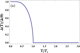
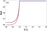
Figure 1: (a) Energy gap $\Delta$ vs temperature $T$ for the conventional superconductor. The energy gap is normalized to its value at the zero temperature while $T$ is measured in the unit of the critical temperature $T_{c}$. (b) The degree of symmetry of $\rho_{S}^{T}$ with respect to the $\mathrm{\mathrm{SO}}(2)$ transformation group. The blue solid and red dashed curves are corresponded to $g(0)k_{B}T_{c}=0.4$ and $0.5$, respectively.

V Quantifying SSB in bosons system

The bosons system can be mapped into the many spin model with the Hamiltonian

$$H_{B} = \xi_{B}\sum_{i=1}^{N}e^{-i\frac{\theta}{2}\sigma_{y}^{i}}\sigma_{z}^{i}e^{i\frac{\theta}{2}\sigma_{y}^{i}},$$ (30)

where

$$\xi_{B}=\sqrt{\epsilon^{2}+\lambda^{2}}, \sin\theta=\lambda/\xi_{B}.$$

In the limit of large $N$ and low excitation, the ground state $\left|G\right\rangle_{B}=\prod_{i=1}^{N}e^{-i\frac{\theta}{2}\sigma_{y}^{i}}\left|\downarrow\right\rangle_{i}$ is approximately equivalent to a coherent state, i.e., $\left|G\right\rangle_{B}\simeq\left|\alpha\right\rangle$, where $\alpha=-\sqrt{N}\theta/2$. It sounds meaningful in physics that the ground state of BEC is also a coherent state as shown in Eq.(13) .

Similar to the case of the BCS theory, we can obtain

$$S(\mathrm{SO}(2)^{\otimes N},H_{B})=1-\frac{\lambda^{2}}{2\left(\epsilon^{2}+\lambda^{2}\right)}.$$ (31)

As $\mathrm{Tr}(\left(\rho_{B}^{T=0}\right)^{2})=1$, the DoS of the ground state reads

$$S(\mathrm{SO}(2)^{\otimes N},\left|G\right\rangle_{B}) = \frac{1}{2}+\frac{1}{2}(1-\frac{\lambda^{2}}{2\xi_{B}^{2}})^{N}.$$ (32)

The order parameter at $T=0$ can be calculated as

$$\left\langle a\right\rangle_{0} =\frac{1}{\sqrt{N}}{}_{B}\left\langle G\right|\sum_{i}\sigma_{-}^{i}\left|G\right\rangle_{B}$$

$$=-\frac{\sqrt{N}}{2}\sin\theta.$$ (33)

Furthermore, the DoS of the ground state can be re-expressed in term of the order parameter,

$$S(\mathrm{SO}(2)^{\otimes N},\left|G\right\rangle_{B})=\frac{1}{2}+\frac{1}{2}(1-\frac{2\left\langle a\right\rangle_{0}^{2}}{N})^{N}.$$ (34)

As $\lim_{x\rightarrow\infty}(1+1/x)^{x}=e$, Eq.(34) is simplified in the limit of large $N$ as

$$\lim_{N/2\left\langle a\right\rangle_{0}^{2}\rightarrow\infty}S(\mathrm{SO}(2)^{\otimes N},\left|G\right\rangle_{B})=\frac{1}{2}+\frac{1}{2}e^{-2\left\langle a\right\rangle_{0}^{2}}.$$ (35)

This is the second main result of this paper, just as the case for the conventional superconductor, the maximum of DoS is directly associated with the vanishing of the order parameter $\langle a\rangle_{0}$. Thus the DoS of the ground state which is less than unity can also indicate the SSB in the bosons system. The same results also hold for the system at finite temperature, since by evaluating Eq.(2) with $\rho_{B}^{T}$ we found

$$S(\mathrm{SO}(2)^{\otimes N},\rho_{B}^{T})=\frac{1}{2}+\frac{\overline{\mathrm{Tr}(R(\omega)\rho R^{\dagger}(\omega)\rho)}_{\mathrm{SO}(2)^{\otimes N}}}{2\mathrm{Tr}\left(\rho^{2}\right)}.$$ (36)

The DoS of $\rho_{B}^{T}$ of BEC is given as follows

$$S(\mathrm{SO}(2)^{\otimes N},\rho_{B}^{T}) = \frac{1}{2}+\frac{1}{2}\left(1-\frac{\lambda^{2}}{2\xi_{B}^{2}}\frac{\cosh\left(2\beta\xi_{B}\right)-1}{\cosh\left(2\beta\xi_{B}\right)}\right)^{N}.$$

Using the approach similar to the above, we rewritten Eq.(LABEL:eq:BEC_T) in terms of the order parameter in a finite temperature $\left\langle a\right\rangle_{T}=\mathrm{Tr}(\rho_{B}^{T}a)=-\lambda\sqrt{N}\tanh(\beta\xi_{B})/(2\xi_{B})$.

$$S(SO(2)^{\otimes N},\rho_{B}^{T}) =\frac{1}{2}+\frac{1}{2}\left[1-\frac{2\left\langle a\right\rangle_{T}^{2}}{N}\frac{1+\cosh\left(2\beta\xi_{B}\right)}{\cosh\left(2\beta\xi_{B}\right)}\right]^{N}.$$

Similar to the absolute zero temperature case, the DoS of $\rho_{B}^{T}$ in bosons system depends both on the order parameter $\left\langle a\right\rangle_{T}$ and the temperature $T$. Just like the Penrose-Onsager criterion 1956 Onsager , the BEC occurs if and only if $\left\langle a\right\rangle_{T}$ is nonzero. When there exists BEC, a large fraction of particles (to the order of $N$) occupy the ground state with zero momentum. When $T>T_{c}$, where $T_{c}$ is the critical temperature of BEC, no condensation occurs. Thus $\left\langle a\right\rangle_{T>T_{c}}=0$, and the symmetry of the bosons system is unbroken.

VI Conclusion

In this paper, we have exploited a measure of symmetry—the degree of symmetry (DoS) to describe the SSB in the conventional superconductor and BEC. We have established rigorous relations between the DoS and the order parameters at the absolute zero temperature and finite temperature. It has been demonstrated that for both the fermions and the bosons systems, (i) at $T=0$, the order parameter takes its maximum and the symmetry of the system is maximally broken; (ii) at $0<T<T_{c}$, the order parameter is still non-vanishing and the extent of the SSB can be quantified by the DoS; (iii) when $T$ grows beyond $T_{c}$, the order parameter vanishes and the symmetry of the system is fully restored.

In fact, the DoS approach that we applied in this paper can be generalized to other circumstances. We can explore symmetry breaking in other quantum many-body systems employing the DoS quantifier and expect to obtain new order parameters when SSB appears. What is worth mentioning is that the new order parameter must be measurable and reasonable in physics.

Appendix A the DoS of the ground state in the fermions system

As shown in Eq.(26), the DoS of the ground state in the fermions system is

$$S(\mathrm{SO}(2)^{\otimes N},\left|G\right\rangle_{S}) =\frac{1}{2}+\frac{1}{2}\prod_{k}\left(1-\frac{1}{2}\sin^{2}\theta_{k}\right)$$

$$=\frac{1}{2}+\frac{1}{2}\exp\left[\sum_{k}\ln\left(1-\frac{1}{2}\sin^{2}\theta_{k}\right)\right]$$

$$=\frac{1}{2}+\frac{1}{2}\exp\left[\int_{-\hbar\omega_{D}}^{\hbar\omega_{D}}g(\epsilon)\ln\left(1-\frac{1}{2}\sin^{2}\theta_{k}\right)d\epsilon\right]$$

$$=\frac{1}{2}+\frac{1}{2}\exp\left[\left|\Delta(0)\right|G(\omega_{D},\left|\Delta(0)\right|)\right]$$ (39)

where

$$G(\omega_{D},\left|\Delta(0)\right|)=\int_{-\frac{\hbar\omega_{D}}{\left|\Delta(0)\right|}}^{\frac{\hbar\omega_{D}}{\left|\Delta(0)\right|}}g(t\left|\Delta(0)\right|)\ln\left(1-\frac{1}{2}\frac{1}{t^{2}+1^{2}}\right)dt,$$

and $\omega_{D}$ is the Debye frequency. As in general case $\hbar\omega_{D}/\left|\Delta(0)\right|\gg 1$ and $g(\epsilon)$ changes slowly in the range of $(-\hbar\omega_{D},\hbar\omega_{D})$, we can take the integral limits to $\pm\infty$ and replace $g(t\left|\Delta(0)\right|)$ with $g(0)$. Therefore, we obtain

$$G(\omega_{D},\left|\Delta(0)\right|) =\int_{-\frac{\hbar\omega_{D}}{\left|\Delta(0)\right|}}^{\frac{\hbar\omega_{D}}{\left|\Delta(0)\right|}}g(t\left|\Delta(0)\right|)\ln\left(1-\frac{1}{2}\frac{1}{t^{2}+1^{2}}\right)dt$$

$$\simeq g(0)\int_{-\infty}^{\infty}\ln\left(1-\frac{1}{2}\frac{1}{t^{2}+1^{2}}\right)dt$$

$$=-(2-\sqrt{2})\pi g(0).$$ (40)

In this sense, the DoS of the ground state in the fermions system is simplified as

$$S(\mathrm{SO}(2)^{\otimes N},\left|G\right\rangle_{S}) =\frac{1}{2}+\frac{1}{2}\exp\left[\left|\Delta(0)\right|G(\omega_{D},\left|\Delta(0)\right|)\right]$$

$$\simeq\frac{1}{2}+\frac{1}{2}\exp\left[-(2-\sqrt{2})\pi g(0)\left|\Delta(0)\right|\right]$$ (41)

References

• (1) Noether, E. Invariante variationsprobleme. Nachrichten von der Gesellschaft der Wissenschaften zu Gottingen 2, 235 (1918).
• (2) T. W. B. Kibble, J. Phys. A: Math. Gen. 9, 1387 (1976).
• (3) W. H. Zurek, Nature 317, 505 (1985).
• (4) T. W. B. Kibble, Symmetry Breaking and Defects, in Patterns of Symmetry Breaking, Eds. H. Arodz, J. Dziarmaga, and W. H. Zurek (Springer, Cracow, 2003).
• (5) Y. Bunkov, Physica B 329, 70 (2003).
• (6) E. H. Lockwood, R. H. Macmillan, Geometric Symmetry, (Cambridge Press, London, 1978).
• (7) Y. Saito and H. Hyuga, Rev. Mod. Phys. 85, 603, (2013).
• (8) J. P. Lowe, Quantum Chemistry, (Academic Press, Boston, 1993).
• (9) V A Miransky, Dynamical Symmetry Breaking In Quantum Field Theories, (World Scientific, 1994).
• (10) T. W. B. Kibble, Phil. Trans. R. Soc. A 373, 33 (2014).
• (11) P. W. Higgs, Phys. Rev. Lett. 13, 508 (1964).
• (12) Z. M. Wang, W. L. Xu, L. Liu, and T. F. Zhu, Nat. Chem. 8, 698 (2016).
• (13) L. D. Landau and E. M. Lifshitz, Statistical Physics Volume One, (Pergamon Press, Oxford, 1969).
• (14) J. Bardeen, L. N. Cooper, J. R. Schrieffer, Phys. Rev. 106, 162 (1957).
• (15) O. Penrose and L. Onsager, Phys. Rev. 104, 576 (1956).
• (16) C. N. Yang, Rev. Mod. Phys. 34, 694 (1962)
• (17) Y. N. Fang, G. H. Dong, D. L. Zhou, C. P. Sun, Commun. Theor. Phys. 65. 423 (2016).
• (18) Yao Yao, G. H. Dong, Xing Xiao, C. P. Sun, arXiv:1605.00789.
• (19) S. Sachdev, Quantum phase transitions, (Cambridge University Press, Cambridge, 1999).
• (20) L. N. Cooper, Phys. Rev. 104, 1189 (1956).
• (21) Kerson Huang, Statistical Mechanics, 2nd ed.,Wiley, New York (1987).