Valence excitation of NO₂ by impulsive stimulated x-ray Raman scattering

Abstract

The global optimum for valence population transfer in the NO₂ molecule driven by impulsive x-ray stimulated Raman scattering of one-femtosecond x-ray pulses tuned below the Oxygen K-edge is determined with the Multiconfiguration Time-Dependent Hartree-Fock method, a fully-correlated first-principles treatment that allows for the ionization of every electron in the molecule. Final valence state populations computed in the fixed-nuclei, nonrelativistic approximation are reported as a function of central wavelength and intensity. The convergence of the calculations with respect to their adjustable parameters is fully tested. Fixing the 1fs duration but varying the central frequency and intensity of the pulse, without chirp, orientation-averaged maximum population transfer of 0.7% to the valence B₁ state is obtained at an intensity of 3.16$\times$10¹⁷ W cm^-2, with the central frequency substantially 6eV red-detuned from the 2nd order optimum; 2.39% is obtained at one specific orientation. The behavior near the global optimum, below the Oxygen K-edge, is consistent with the mechanism of nonresonant Raman transitions driven by the near-edge fine structure oscillator strength.

I Introduction

Recently there have been proposals for using multiple attosecond x-ray pulses to study the quantum dynamics of valence electronic excitations in molecules Biggs et al. (2012); Mukamel et al. (2013). These techniques, called multidimensional attosecond x-ray spectroscopy, promise to provide an unparalleled, time-resolved picture of evolving electronic and internuclear nuclear structures. Pump-probe experiments using ultrafast pulses of x-ray light have already provided a time-resolved picture of the evolving electronic and nuclear dynamics in several important systems [CITE GESSNER]. The amount of information that the proposed, more sophisticated multidimensional spectroscopic methods will provide is much greater. The multidimensional methods offer the chance to observe the quantum dynamics of multiple degrees of freedom, extracting the correlations among electrons and nuclei that comprise much of atomic, molecular, and chemical physics, observing and manipulating electronic coherences in the molecule. For instance, the coupled electronic and nuclear dynamics in chromophores [CITE] involves correlated motion of several electrons, and there is an active effort to develop better chromophores synthetically. Experimental methods that allow quantum correlations and coherences to be observed and manipulated directly are invaluable for technological advancement.

The essential benefit of x-ray wavelengths lies in their elemental and chemical specificity, as demonstrated by recent work [CITE pi/pi*]. By creating, combining and interfering physically localized excitons in a molecule, which then evolve, multidimensional x-ray spectroscopies offer the promise of disentangling correlations in time and space. Many of the proposals for multidimensional x-ray spectroscopy rely on the creation of a coherent valence electronic wavepacket using nominally two-photon, stimulated x-ray Raman transitions. Valence excitations are most relevant to real-world applications; therefore, x-ray Raman methods are particularly attractive. Furthermore, they may be implemented without regard to the relative coherence of the multiple attosecond pulses. The broadband x-ray pulses drive the impulsive stimulated Raman process, the excitation via the pump frequencies and the stimulated emission of Stokes frequencies, leading to a coherent valence electronic excitation. The 1D- and 2D-SXRS multidimensional spectroscopies Biggs et al. (2012); Mukamel et al. (2013) combine several such excitations, and are capable of obtaining time- and frequency-resolved information about electronic structure and couplings and about the evolving internuclear geometry.

These proposed methods require further evolution of laser technology in order to become viable. Considerable investment is being made in next-generation light sources, both in high-harmonic generation and free-electron lasers, and theory may provide guidance for these investments. Given the investment and effort required to construct these experiments, reliable, comprehensive and unbiased theoretical predictions may provide valuable guidance.

Providing accurate theoretical predictions for these experiments is difficult, however, due to the number of electrons involved in the intense-field dynamics including core excitations, and due the inherent exponential scaling of quantum mechanical problems with respect to system size. There have been several sophisticated theoretical and computational studies of multidimensional X-ray spectroscopic and related methods including Refs. Biggs et al. (2013a, b); Kirrander et al. (2016); Miyabe and Bucksbaum (2015). However, these studies have often concentrated on electronic excitations to metastable core-excited states and neglected the continuum above the edge, and often they have explicitly computed the nth-order signal without considering large-magnitude higher-order behavior that might overwhelm lower orders even at low intensity.

For these reasons it is desirable to test the efficiency of impulsive stimulated x-ray Raman transitions in polyatomic molecules in a fully nonperturbative, first-principles calculation that accounts for all the fundamental effects including multiple ionization, stark shifts, and highly correlated electronic dynamics. X-ray Raman transitions involve correlation of many electrons, because the excitation of the inner, core electrons affects the field experienced by the other electrons, and because the Auger decay of the intermediate states involves transitions of two electrons or more. The intense field may directly excite or ionize many electrons. Prior treatment of strong x-ray effects like cation charge state yields have employed rate equation models using thousands or millions of electronic configurations [CITE]. In contrast, the treatment of the coherent process of stimulated electronic x-ray Raman transitions requires a coherent, wave function description.

The Multiconfiguration time-dependent Hartree-Fock (MCTDHF) method Kitzler et al. (2004); Kato and Kono (2004); Caillat et al. (2005); Nest et al. (2005); Alon et al. (2007); Nest et al. (2007, 2008); Kato and Kono (2008); Nest (2009); Kato and Yamanouchi (2009); Kato et al. (2009); Miyagi and Madsen (2013); Sato and Ishikawa (2013, 2015); Sawada et al. (2016) is in principle capable of calculating arbitrary nonperturbative quantum dynamics of electrons in medium-sized molecules, with all electrons active and able to be ionized. The “Hartree-Fock” part of the name makes it a misnomer, because MCTDHF employs a systematic expansion of the wave function in terms of a time-dependent linear combination of time-dependent Slater determinants that converges to the exact solution in the limit of many orbitals and determinants. We speculate that current technology permits converged calculations of fixed-nuclei, electronic dynamics of organic molecules at the limits of intensity, using the MCTDHF method, and we provide evidence for this contention in this article.

We have applied our implementation of MCTDHF Haxton et al. (2011); Haxton and McCurdy (2015); Jones et al. (2016); Haxton et al. to predict transfer of population to valence excited electronic states due to stimulated X-ray transitions in the NO₂ molecule, in the fixed-nuclei approximation. This implementation includes a polyatomic representation in which the scaling in terms of three-dimensional system size (times the maximum nuclear charge, due to the discretization required for the nuclear cusp, for explicitly-represented core electrons) is linear times logarithmic, in other words, order $N\log{N}$. It allows for several million Slater determinants – a number that may be greatly increased with current technology – with an arbitrary Slater determinant space. Flexible spaces involving different shells and excitations can be defined, and we demonstrate the convergence of the results here with respect to the orbital and Slater determinant basis. These MCTDHF calculations test the viability of impulsive Raman transitions for driving valence electronic state population transfer without making any assumptions about the degree of electronic excitation, correlation, or ionization, nor about the number of photons absorbed and emitted, using a quantum mechanically coherent representation.

We show that in the NO₂ molecule, for impulsive stimulated x-ray Raman scattering using 1fs pulses, transitions to the ²B₁ valence electronic state dominate. Population transfer of 0.70% may be driven at 2nd order by tuning below the near-edge fine structure, as in Ref. Miyabe and Bucksbaum (2015), without orienting the molecule, and 2.39% or more population can be transferred once the molecule is oriented. However, nonlinear effects quickly set in above 10¹⁶ W cm^-2, and a global optimization of population transfer as a function of intensity and central frequencies appears to be driven by nonresonant Raman transitions, substantially red-detuned from the near-edge fine structure, a mechanism not considered in Ref. Miyabe and Bucksbaum (2015).

The results indicate that multidimensional attosecond electronic X-ray Raman spectroscopies might in general most efficiently be performed using pulses well red-detuned from resonant edges. Such pulses may minimize loss through direct and sequential ionization and make use of the coherent combination of discrete and continuum edge oscillator strength, thereby providing the greatest potential for creating coherent valence electronic wave packets through impulsive stimulated x-ray Raman excitation. Strong red-detuning may provide a way to efficiently perform stimulated Raman transitions in molecules, because it prevents an excursion of the 1s electron.

II MCTDHF method and representation of NO₂

Briefly, the MCTDHF method Kitzler et al. (2004); Kato and Kono (2004); Caillat et al. (2005); Nest et al. (2005); Alon et al. (2007); Nest et al. (2007, 2008); Kato and Kono (2008); Nest (2009); Kato and Yamanouchi (2009); Kato et al. (2009); Miyagi and Madsen (2013); Sato and Ishikawa (2013, 2015); Sawada et al. (2016) solves the time-dependent Schrodinger equation using a time-dependent linear combination of Slater determinants, with time-dependent orbitals in the Slater determinants. The nonlinear working equations are obtained through application of the Lagrangian variational principle Broeckhove et al. (1988); Ohta (2004) to this wave function ansatz.

Our implementation of MCTDHF Haxton et al. for electrons in molecules has already been described Haxton et al. (2011); Haxton and McCurdy (2015); Jones et al. (2016). The representation of orbitals, the one-electron basis, using sinc basis functions is described in Ref. Jones et al. (2016). For NO₂, we use a grid of 55$\times$55$\times$55 ($=$166375) product sinc basis functions for the orbitals. The spacing between the functions is 0.2975614 bohr (about 0.56 Angstrom). As we discuss below, this large grid spacing leads to a substantial error in the Oxygen 1$s$ ionization energy. For comparison, we perform a few calculations using half grid spacing, 0.1487807 bohr, and a 111x111x111 grid of Cartesian sinc basis functions. These finer-resolution calculations allow us to obtain a shift that we can apply to all the coarser-grid results. As mentioned below in the photoionization section, this shift is 2.42eV (about 66eV). We report energies for the coarser grid calculations, and also shifted values in parenthesis and italics, such as “the excitation energy of the XX to YY is ZZZ (xxxx) eV.”

For the Slater determinant list defining the many-electron basis, we use full configuration interaction, 23 electrons in 15 orbitals, giving 621075 Slater determinants which are contracted to 305760 spin-adapted linear combinations and distributed among processors. The mean field time step was 0.02 atomic time units (approximately one half attosecond).

Complex coordinate scaling and stretching Simon (1979) is applied starting at $\pm$4 bohr in the $x$, $y$, and $z$ directions. We perform the smooth complex scaling transformation upon the kinetic energy and derivative operators only. Lacking a viable method for defining the transformed two-electron operator, we do not transform the Coulomb operators. The complex ray is defined as

$$\begin{array}[]{rll}X(x)=&x+a(x-x_{0})+b\sin\left(\pi\frac{x-x_{0}}{x_{1}-x_{0}}\right)\\ &+c\sin^{3}\left(\pi\frac{x-x_{0}}{x_{1}-x_{0}}\right)&(x_{0}\leq x\leq x_{1})\\ =&x+a(x+x_{0})+b\sin\left(\pi\frac{x+x_{0}}{x_{1}-x_{0}}\right)\\ &+c\sin^{3}\left(\pi\frac{x+x_{0}}{x_{1}-x_{0}}\right)&(-x_{1}\leq x\leq-x_{0})\\ =&x&(-x_{0}\leq x\leq x_{0})\end{array}$$ (1)

in which $X(x)$ defines the complex coordinate ray $X$ along which the wave function is defined as a function of the real-valued parameter $x$ in which the operators are represented. Smooth scaling occurs between the scaling boundary $x_{0}=4a_{0}$ and the end of the grid $x_{1}\approx 8.78a_{0}$. The parameters $a$, $b$, and $c$ are determined by the scaling angle and stretching factor (half a radian and three, respectively, such that $X^{\prime}(x)=4e^{0.5i}$ at $\pm x_{1}$) and by making the fourth derivative $X^{\prime\prime\prime\prime}(x)$ continuous. This transformation defines the new length-gauge dipole operators $X$, $Y$, and $Z$, and the DVR weights in each Cartesian direction (originally uniformly $w_{i}=\frac{1}{\Delta}$ with $\Delta$ the sinc DVR spacing) are modified according to $w_{i}\rightarrow X^{\prime}(x_{i})w_{i}$. The first derivative operator matrix elements are transformed as e.g. $(d/dX)_{ij}=(d/dx)_{ij}(X^{\prime}(x_{i})X^{\prime}(x_{j}))^{-1/2}$, and the kinetic energy matrix elements are defined in the DVR approximation as

$$\begin{array}[]{ll}\left(\frac{\partial^{2}}{\partial X^{2}}\right)_{ij}=&\frac{1}{X^{\prime}(x_{i})X^{\prime}(x_{j})}\left(\frac{\partial^{2}}{\partial x^{2}}\right)_{ij}\\ &-\delta_{ij}\frac{3X^{\prime\prime}(x_{i})^{2}-2X^{\prime\prime\prime}(x)X^{\prime}(x_{i})}{4X^{\prime}(x_{i})^{4}}\end{array}$$ (2)

Below in section V we demonstrate the convergence of the population transfer results with respect to the parameters of the exterior complex scaling ray.

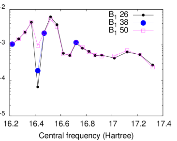
Figure 1: (Color online) Convergence of the $B_{1}$ population at 10¹⁷ W cm^-2, with respect to the order of the Lebedev quadrature used for the orientation average of fixed-nuclei calculations.

III MCTDHF calculation of impulsive Raman population transfer in NO₂

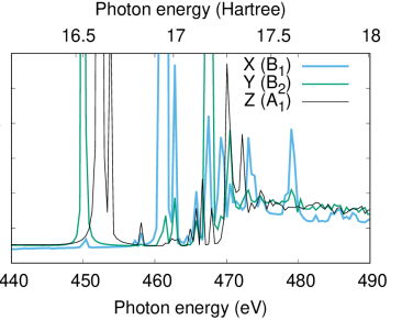
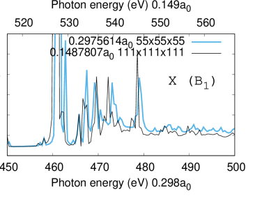
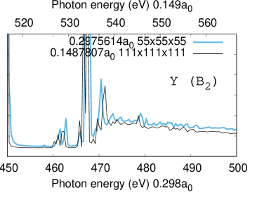
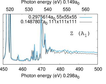
Figure 2: (Color online) NO₂ photoabsorption cross section calculated in the vicinity of the Oxygen K-edge using a 10fs MCTDHF calculation with a weak pulse. The top panel shows results in all three polarizations for the larger 0.2975614$a_{0}$ grid resolution, 55x55x55 grid that we use for most of the calculations in this paper. The oxygen K-edge is artificially low in these calculations. The results with higher 0.1487807$a_{0}$ resolution, 111x111x111 grid for $x$ polarization are shown in the bottom panels, compared with the lower-resolution calculations. The scales on the top and bottom for the two data sets in the bottom panels are relatively shifted by 2.42 Hartree, approximately 66eV, which is the shift that we use when reporting the parenthetical and italicized energies for comparison with experiment, in the body of the text.

We employ a pulse in the dipole approximation with central frequency $\omega$ and duration $\pi/\Omega$ as follows. In the velocity gauge we define the vector potential

$$A(t)=\sin^{2}(\Omega t)\sin\left(\omega\left[t-\frac{\pi}{2\Omega}\right]\right)\quad(0\leq t\leq\frac{\pi}{\Omega})$$ (3)

In the length gauge we employ the electric field $E(t)=\frac{\partial}{\partial t}A(t)$. For the pulses used here, with 1fs full width at half-maximum (FWHM) in time ($\pi/\Omega=$ 2fs), the FWHM of the spectral profile, the squared Fourier transform $|E_{z}(\omega)|^{2}$ is 3.25eV.

We calculate population transfer for the valence B₁, B₂, and A₂ states. We integrate the result over orientations using Lebedev quadrature Lebedev (1975, 1976, 1977); Lebedev and Skorokhodov (1992); Lebedev and Laikov (1999). Comparing 38- and 50-point quadrature, we find that most of the results are converged with 38-point quadrature. We have not attempted to demonstrate the convergence of these results beyond 50-point quadrature due to computer resources. In Figure 1 we show the convergence of the $B_{1}$ population at 10¹⁷ W cm^-2, with respect to the order of the Lebedev quadrature. The convergence is good where the population transfer is large, but the sharp minimum in the population transfer at 16.4 Hartree requires more points for full convergence.

Due to symmetry, and within the rotating wave approximation, only seven of the 50 points need to be calculated. Each central frequency and intensity required approximately 10,000 cpu-hours to calculate: seven calculations, 121 processors each, and about twelve hours per calculation.

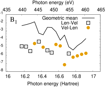
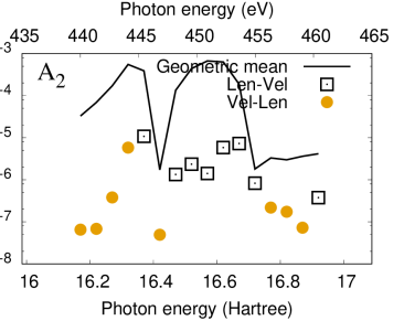
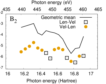
Figure 3: (Color online) Comparison of population transfer calculated in length and velocity gauge, at 3.16 $\times$ 10¹⁷ W cm^-2, calculated at the larger 0.2975614$a_{0}$ grid resolution, presented in order to facilitate a judgment of the effect of discretization error and the convergence of the result with respect to the spacing between adjacent sinc basis functions. The geometric means of the length and velocity gauge population transfer results are plotted along with their differences. Black squares and grey (orange) dots indicate that the sign of the difference between length and velocity is positive and negative, respectively.

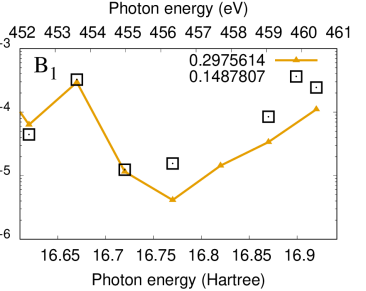
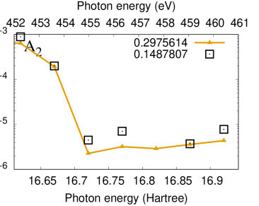
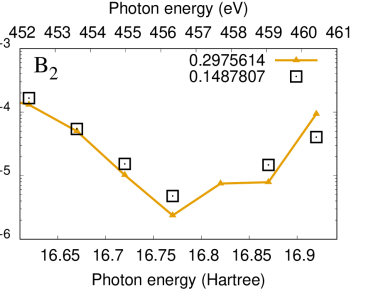
Figure 4: (Color online) Convergence with respect to grid resolution. The populations for the calculation with polarization vector 45 degrees relative to the principal axes of the molecule, i.e. not averaged over orientations, calculated at 3.16 $\times$ 10¹⁷ W cm^-2, are shown at two resolutions, 0.2975614$a_{0}$ grid resolution like most of the calculations in this paper, and the smaller 0.1487807$a_{0}$, with grid sizes 55x55x55 and 111x111x111.

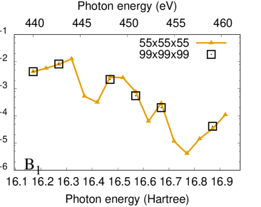
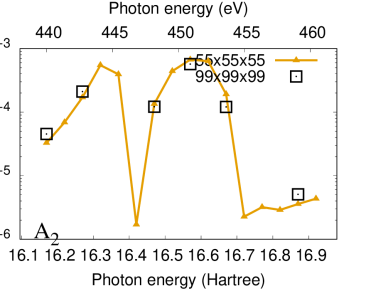
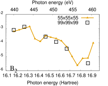
Figure 5: (Color online) Convergence with respect to primitive sinc DVR basis set, at fixed resolution. The populations for the calculation with polarization vector 45 degrees relative to the principal axes of the molecule, i.e. not averaged over orientations, calculated at 3.16 $\times$ 10¹⁷ W cm^-2 using the 55x55x55 basis used for most of this paper, are compared with populations calculated with a larger 99x99x99 basis and larger complex coordinate scaling radius, as described in the text.

IV Photoionization cross section

Fig. 2 shows the photoabsorption cross section calculated in the neighborhood of the Oxygen K-edge. This figure demonstrates that the the one-photon transition amplitudes that drive the Raman process are accurately reproduced, although there are some significant shifts in the positions of the peaks corresponding to autoionizing states that comprise the near-edge fine structure.

The bottom panel of this figure shows a higher-resolution result superimposed on the result from the lower-resolution calculation that is used for the majority of the calculations in this paper. The resolution is doubled to 0.1487807 bohr, with a 111x111x111 sinc DVR basis set. This comparison shows that the excitations are accurately reproduced at the lower resolution, except for the substantial overall shift in the x-axis values. The higher-resolution calculation appears to accurately reproduce the location of the experimentally-observed edge [CITE], which is obscured and broadened by the overlapping fine structure and by nuclear motion, around 535eV. The shift that is required to make the results at the higher and lower resolutions coincide, the shift used in defining the x-axis ranges in the bottom panel of Fig. 2, is 2.42 Hartree, approximately 66eV. We use this shift, 2.42 Hartree or 66eV, when defining shifted numbers throughout the remainder of the text. We report the energies from the lower-resolution calculation, and include parenthetical italicized shifted numbers, using 2.42 or 66eV. For instance, “the excitation energy of the XX to YY is ZZZ (xxxx) eV.”

The magnitude of the cross section above and below the edge (about 0.5 and a bit more than 1.0 respectively) agree well with figure 5.10 in Berkowitz’s compilation Berkowitz (2002). The three peaks at about 450 ($A_{1}$), and 452 & 453 ($B_{1}$) correspond to excitations to $6a_{1}$ and $2b_{1}$ from the Oxygen 1s $\sigma_{g}$ orbital, and correspond with the peaks observed at approximately 530, 532, and 533 in experiment Jurgensen and Cavell (2000); Gejo et al. (2003); Piancastelli et al. (2004). Relative to these peaks, there is also a pair of $B_{2}$ states, at about 462eV, both spin couplings for excitation to $5b_{2}$, and the K-edge lies at about 468-470eV. It is clear that the K-edge is too high in energy, and the $B_{2}$ states are too low, because the $B_{2}$ states are observed as a broad core-excited shape resonance in experiment. Experiment Jurgensen and Cavell (2000); Gejo et al. (2003); Piancastelli et al. (2004) gives a $A_{1}$ to $B_{2}$ excitation energy of 15eV, and a K-edge about 12eV above $A_{1}$; here they are found at about 12 and 18eV, respectively.

Because the shift in the Oxygen K-edge means that the Oxygen and Nitrogen K-edges are unphysically close, one would expect that the loss due to ionization of the Nitrogen 1$s$ electron would be enhanced and therefore that the population transfer would be underestimated as a result of this discretization error. However, the cross sections above and below the Oxygen K-edge have the correct magnitude, so the effect of the artificial shift in the Oxygen K-edge may in fact be small. The higher-resolution $111\times 111\times 111$ calculations shown in the bottom panel of Fig. 2 demonstrate that all aspects of the first-order photoionization result are converged at the lower resolution, except for the substantial shift in the K-edge energy.

V Further tests of convergence with respect to single-electron basis

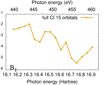
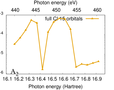
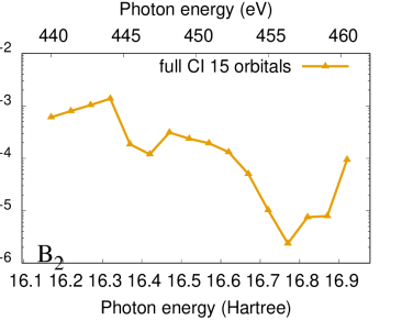
Figure 6: (Color online) Convergence with respect to Slater determinant (many-electron) representation. The populations for the calculation with polarization vector 45 degrees relative to the principal axes of the molecule, i.e. not averaged over orientations, calculated at 3.16 $\times$ 10¹⁷ W cm^-2 using the 55x55x55 basis used for most of this paper, are compared with populations calculated with the alternate orbital and Slater determinant basis described in Sec. VI.

The main approximations in these calculations are the omission of nuclear motion, the discretization via sinc functions, and the omission of relativistic (broadly speaking, non-dipole) effects. The last is the most severe, and will be tested in subsequent work. Otherwise, the results for population transfer with fixed nuclei should closely correspond to the physical result for electronic state population transfer, because the nitrogen and oxygen atoms are expected to move very little over the one-femtosecond duration of the pulse. At the limits of intensity, non-dipole effects may become significant and future work will examine their effect on impulsive Raman transitions.

As discussed in the section above, the error due to discretization (grid resolution) appears to be small, based on the first-order results, beyond the substantial shift in the Oxygen K-shell 1$s$ ionization energy. The first-order behavior is converged, except for the shift. The spacing of the sinc functions (0.2975614 $a_{0}$) is sufficient to represent plane waves with an energy up to 6 keV, so the wave function in the asymptotic region does not suffer from any discretization error. The only error due to discretization is due to the cusps in the electronic wave function at the nuclei.

In order to more fully judge the effect of the discretization error at the cusps at the nuclei for the nonlinear population transfer process, we compare the results of length and velocity gauge in Fig 3. As the spacing between adjacent sinc basis functions goes to zero, the difference between length and velocity gauge also goes to zero. Therefore, the difference between length and velocity gauge gives error bars for the results.

Velocity gauge calculations place a greater emphasis on the wave function near the nuclei, whereas length gauge calculations place greater weight on the long-range wave function. Therefore, we regard length gauge calculations to be more reliable.

However, the issue is moot because, like the lowest-order photoionization results presented in the section above, the agreement between length and velocity gauge for the nonlinear population transfer result, demonstrated in Fig 3, is quite good. Given the large spacing between sinc functions – again, 0.2975614 $a_{0}$ – this agreement may be surprising. The sinc basis functions do not accurately represent the cusp at the nucleus, and as demonstrated in Fig. 2, the position of the Oxygen K-edge has a substantial error. However, despite these considerations, the results for population transfer in Fig. 3 in length and velocity gauge in Fig have an agreement of better than one part in ten (10%) to 1000 (0.1%) .

As demonstrated in Ref. Jones et al. (2016), the discrete variable representation (DVR) approximation to the Coulomb matrix elements, involving the inverse of the kinetic energy matrix, gives results that are far superior to the variational method. Because this DVR approximation is not variational, considerations based on the smoothing of the cusp at the nucleus do not necessarily apply. As demonstrated in Ref. Jones et al. (2016), much better results are obtained with the nonvariational DVR approximation in Ref. Jones et al. (2016) than with the variational method. The DVR approximation for the Coulomb matrix elements described in Ref. Jones et al. (2016) preserves the relationship between the kinetic energy and the Coulomb operator – the Coulomb operator is the integral kernel of the inverse of the kinetic energy operator – in matrix form. We speculated that the preservation of this relationship is responsible for the surprising accuracy of virial theorem ratios presented in Ref. Jones et al. (2016), and we also speculate that it is responsible for the surprising agreement between length and velocity gauge presented in Fig. 3.

We present an explicit demonstration of convergence with respect to grid resolution in Fig. 4. The resolution is doubled and everything else is kept constant. The spacing is halved to 0.1487807$a_{0}$ and the grid is doubled to $111\times 111\times 111$. Only one calculation for the orientation average is shown, the one corresponding to the Lebedev quadrature point for which the polarization vector is parallel with the vector $(x,y,z)=(1,1,1)$, in which $x,y,z$ are principal (c_2V) axes of the molecule, and only a few calculations have been performed due to limited computer resources. These few calculations however show good convergence, well within an order of magnitude. Better convergence might be found by slightly adjusting the intensity, because small differences in first-order transition strengths are magnified in a nonlinear process. Further work is required for a more complete study of the convergence with respect to grid resolution, including the orientation average required to predict the observed result.

In Fig. 5, we demonstrate the convergence with respect to the sinc DVR orbital basis, keeping the resolution fixed. Again, only the polarization vector $(x,y,z)=(1,1,1)$ calculation is performed, not the entire orientation average. The convergence with respect to the extent of the grid and the exterior smooth complex coordinate scaling is tested by comparing the results from the $55\times 55\times 55$ calcuation with complex scaling starting at $x$, $y$, or $z=4a_{0}$, with results obtained from a larger $99\times 99\times 99$ calculation with complex scaling starting at $x=a_{0}$ and extended to $x=14a_{0}$, in which $x$ is the real-valued coordinate that parameterizes the complex-valued ray. The stretching factor and scaling angle were kept at their previous values of 3 and 0.5 radians (about 60 degrees). The agreement of the results is good, with ten percent.

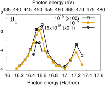
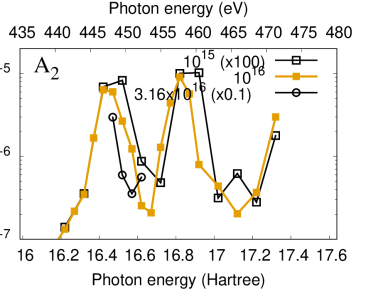
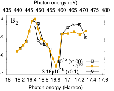
Figure 7: (Color online) Behavior of population transfer at low intensity. Different intensities are plotted with different lines and labeled in Watts per square centimeter. The results at 10¹⁵ and 3.6 $\times$ 10¹⁶ Watts per square centimeter have been multiplied by factors to facilitate a comparison of the generalized two-photon cross section. To obtain a generalized two-photon cross section in megabarns squared $\times$ femtoseconds, multiply the plotted y-axis value by 345 times the x-axis value squared.

VI Convergence with respect to many-electron basis

The many-electron convergence is tested by varying the orbital and Slater determinant basis. The MCTDHF method employs time-dependent orbitals and therefore every electron can be simultaneously excited, regardless of the Slater determinant space. The defects imposed upon the time-dependent MCTDHF solution by the truncation of the Slater determinant space are not yet understood, and different in nature from those due to truncated time-independent Slater determinant basis sets.

Furthermore, the nature of these defects must be intimately tied to the chosen variational principle. The coupling terms among orbitals are dictated by the chosen variational principle, and these coupling terms distinguish different MCTDHF methods involving truncated Slater determinant spaces. However, these terms are often approximated [CITE,CITE] are entirely neglected [CITE,CITE]. We have provided a derivation of explicit working equations for the McLachlan and Lagrangian variational principles Haxton and McCurdy (2015). Those working equations are employed in the tests reported here – specifically, the method that mixes 10% McLachlan with 90% Lagrangian.

In general, we find Haxton and McCurdy (2015) that the time-independent many-electron basis sets used in contemporary MCSCF (multiconfiguration self-consistent field) and configuration-interaction, and also in configuration-interaction representations of time-dependent problems, do not behave well in the MCTDHF method Haxton and McCurdy (2015), following either the Lagrangian (least action) or McLachlan (minimum norm of the error) stationary principle. Symmetry breaking is more severe Haxton and McCurdy (2015) using typical Slater determinant sets such as CISD (configuration interaction with single and double excitations). We have found Haxton and McCurdy (2015) that the particle-hole conjugates of these basis sets, corresponding to a full configuration outer shell with a few excitations allowed from the core, perform best.

However, here we expand the orbital basis greatly, from 15 to 20 orbitals, in order to fully test the convergence with respect to orbitals, and employ a CISD slater determinant space. We divide the 20 orbitals into two shells of 11 and 9. The wave function is represented using CIS, single transitions only from the first 11 to the last 9 time-dependent orbitals. Matrix elements are computed among the CISD determinant space. 18 to 20 electrons are allowed in the first shell and one to three electrons in the second. In total, only 1296 spin-adapted linear combinations of Slater determinants are explicitly included in the CIS representation, and matrix elements among 62940 CISD Slater determinants are recomputed each time step. Essentially all of the time in this calculation is spent propagating orbitals.

In comparison, for the rest of the calculations in this paper we use full configuration interaction with 23 orbitals, yielding 621075 spin-adapted linear combinations of Slater determinants. The two calculations, 15-orbital full configuration and 20-orbital CISD, are very different and agreement between these calculations would strongly imply convergence with respect to the Slater determinant representation.

In Fig. 6, we show

BLAH

BLAH

BLAH

BLAH

BLAH

BLAH

BLAH

VII Low-intensity behavior

The behavior of the population transfer at relatively low intensity is shown in Fig. 7. This figure shows the population transfer at intensities for which the second-order behavior begins to break down. Intensities of 1$\times$10¹⁵ W cm^-2, 1$\times$10¹⁶ W cm^-2, and 3.16$\times$10¹⁶ W cm^-2 are plotted, and the first and last of these are multiplied by factors of 100 and 0.1, respectively, in order to judge the degree to which second-order behavior is obeyed. If second-order perturbation theory were to hold for these intensities, the lines in Fig. 7 would coincide.

In this figure one can see that the behavior is still second-order at an intensity of 1$\times$10¹⁶ W cm^-2 for the lower photon energies, below about 447eV, because the lines corresponding to 1$\times$10¹⁶ W cm^-2 and 1$\times$10¹⁵ W cm^-2 coincide in that region, on the left side of the figures. Above 447eV, these two lines diverge, so it is clear that the behavior at 1$\times$10¹⁶ W cm^-2 is beyond second-order when the central frequency is close and above the near-edge fine structure and Oxygen K-edge.

The low-intensity behavior in Fig. 7 mirrors what is expected from second-order perturbation theory. The optimum population transfer at low energy occurs at about 450eV for the B₁ state, and about 447eV for the B₂ state. For the A₂ state, for which the population transfer is smaller, there are a pair of local maxima at about 447 and 458eV.

The mechanisms for population transfer can be inferred by reference to Fig. 2, which shows the photoionization cross section. In that figure, there is an A₁ metastable state at about 450eV, a pair of B₁ states at about 452 and 453eV; and a pair of B₂ states at about 461 and 462eV. The Oxygen K-edge is obscured by additional peaks corresponding to metastable states, but the edge seems to occur at about 470eV.

Because the optimum population transfer at low intensity occurs far below the edge, relative to the spectral bandwidth of 3.25eV, it is clear that the transitions are driven through the metastable, discrete autoionizing states comprising the near-edge fine structure at low intensity. This low-intensity behavior for 1fs FWHM pulses is consistent with the picture presented in Ref. Miyabe and Bucksbaum (2015).

The Hartree-Fock configuration of the initial ground state is $1a_{1}^{2}2a_{1}^{2}1b_{2}^{2}3a_{1}^{2}2b_{2}^{2}4a_{1}^{2}3b_{2}^{2}5a_{1}^{2}1b_{1}^{2}4b_{2}^{2}1a_{2}^{2}6a_{1}^{1}$. The metastable states comprising the near-edge fine structure that are visible as the most prominent peaks in Fig. 2, A₁, B₁, and B₂, and which have been observed in experiment Jurgensen and Cavell (2000); Gejo et al. (2003); Piancastelli et al. (2004) are described as excitations $1a_{1}\rightarrow 6a_{1}$, $1a_{1}\rightarrow 2b_{1}$, and $1a_{1}\rightarrow 5b_{2}$. The valence B₁, A₂, and B₂ states are described as excitations $6a_{1}\rightarrow 2b_{1}$, $1a_{2}\rightarrow 6a_{1}$, and $4b_{2}\rightarrow 6a_{1}$.

The optimum at 450eV for population transfer to the valence B₁ state in Fig. 7 is consistent with two-photon transitions via the intermediate B₁ states, proceeding as $1a_{1}\rightarrow 2b_{1}$, $6a_{1}\rightarrow 1a_{1}$. In the photoionization cross section in Fig. 2, the two ($1a_{1}\rightarrow 2b_{1}$) ${}^{2}B_{1}$ states at 452 and 453eV have the same orbital occupancy but different spin parentage. They are described most closely as states in which the singly-occupied $2b_{1}$ and $6a_{1}$ orbitals are singlet or triplet coupled. The triplet-coupled $1a_{1}^{-1}6a_{1}^{1}2b_{1}^{1}$ B₁ intermediate state at 453eV, with a smaller oscillator strength (smaller peak) in Fig. 2, is that which drives the Raman transition.

The A₁ state at 450eV ($1a_{1}\rightarrow 6a_{1}$) is not expected to contribute because the subsequent transition downward would involve the transition of more than one electron in the Hartree-Fock picture. In Fig. 2 it is clear that the oscillator strength from the ground state to the B₁ state at 452eV is greatest among these three, and the 450eV optimum is most closely consistent with a transition via a 452eV intermediate state, given the 3.25eV bandwidth.

The 447eV optimum for population transfer to the valence B₂ state in Fig. 7 is consistent with a transition through the lowest A₁ metastable state at 450eV, proceeding as $1a_{1}\rightarrow 6a_{1}$, $4b_{2}\rightarrow 1a_{1}$. A two-photon transition via the intermediate B₁ state is not dipole-allowed. There is no second maximum corresponding to population transfer via the intermediate B₂ state ($1a_{1}\rightarrow 5b_{2}$) at higher energy because the Stokes transition would require moving more than one electron in the Hartree-Fock picture.

The A₂ valence state population transfer at low intensity seen in Fig. 7 has two maxima, at about 447 and 458eV. The higher-photon-energy 458eV maximum is slightly greater. Both of these maxima are lower for this A₂ state (population transfer equal or less than 10^-5 at 10¹⁶ W cm^-2) than the maxima for B₁ (over 10^-3 at 10¹⁶ W cm^-2) and B₂ (about 10^-4 at 10¹⁶ W cm^-2). The lower population transfer for the valence A₂ state is consistent with a transition driven by configuration mixing in the intermediate or final state. The $1a_{2}\rightarrow 6a_{1}$ configuration of the valence A₂ state cannot be obtained by two subsequent dipole-allowed one-electron transitions involving the 1$s$ electrons. Transitions through the lower B₁ states at 450 and 452eV ($1a_{1}\rightarrow 2b_{1}$) and through the B₂ states at 461 and 462eV ($1a_{1}\rightarrow 5b_{2}$) are clearly responsible for the population transfer to this A₂ valence state, given the location of the two sharp maxima for population transfer at about 447 and 458eV. The low value of the population transfer at these maxima is explained by the fact that the subsequent transition to the final $1a_{2}\rightarrow 6a_{1}$ configuration is driven by configuration mixing in these states, the intermediate B₂ and B₁ or the final A₂. Correlating excitations $1a_{2}5b_{2}\rightarrow 6a_{1}2b_{1}$ and $1a_{2}2b_{1}\rightarrow 6a_{1}5b_{2}$ in the B₂ and B₁ intermediate state are the most probable explanations of the calculated population transfer.

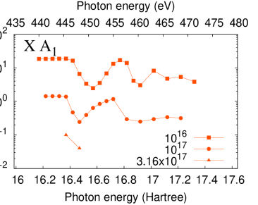
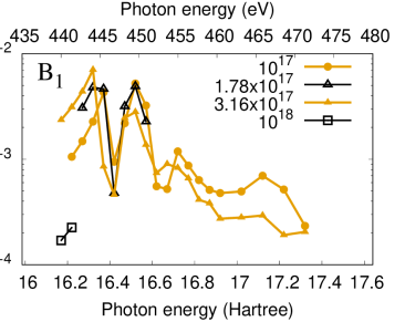
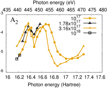
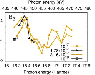
Figure 8: (Color online) Results for population transfer to the B₁, A₂, and B₂ valence excited states of NO₂, and odds for remaining in the ground state, averaged over orientation, for 1fs pulses, at higher intensities showing the global optimum population transfer. Different intensities are plotted with different lines and labeled in Watts per square centimeter.

VIII Optimizing impulsive X-ray Raman excitation of NO₂

These results are limited to linearly polarized 1fs FWHM pulses. Such pulses are expected to be available from free-electron lasers in the near future. In order to further examine the parameter space to find the truly global optimum for impulsive x-ray Raman population transfer, we will vary chirp and duration in future work.

The results for population transfer at high intensity, including the global optimum, for these 1fs FWHM linearly polarized pulses near the Oxygen $1s$ K-edge, are shown in Figure 8.

The best population transfer is obtained for the B₁ state, at the intensity 3.16$\times$10¹⁷ W cm^-2 and approximately 444.1eV (16.32 Hartree) photon energy, substantially 6eV red-detuned from the second-order optimum which occurred at 450eV as described above. However the optimum population transfer is only 0.70% with these one-femtosecond, linearly polarized pulses, for the orientation average. Among the seven distinct Lebedev quadrature points required to compute the 50th order orientation average, the largest population transfer to the B₁ state was at this intensity and central frequency, 3.16$\times$10¹⁷ W cm^-2 and 6.32 Hartree, at 2.39%. This optimum was obtained for the fixed orientation with a polarization vector $(x,y,z)=(0,1,1)$ in the molecular frame, in which $(x,y,z)$ are the principal axes of the molecule and $x$ is perpendicular to the plane of the molecule.

In a well-designed multidimensional spectroscopy experiment, the efficiency of subsequent steps benefits from the orientation imparted by prior steps. The 2.39% population transfer maximum, greatest among the orientations that we calculated, implies a coherence as great as 15%, which would easily enable proposed multidimensional attosecond x-ray spectroscopy experiments. The cleanest experiment would be performed at a lesser intensity, to reduce noise. These calculations indicate that there is no fundamental limitation to the implementation of proposed multidimensional attosecond x-ray spectroscopy methods, based on the efficiency of the population transfer with 1fs pulses.

Examining the population transfer for B₁, going from low intensity in Fig. 7 to high intensity in Fig. 8, one can see that a minimum develops at about 446eV. The peak population transfer does not shift monotonically downward as intensity is increased. Instead, this sharp minimum at about 446eV develops, the original peak at 450eV saturates at about 1.78$\times$10¹⁷ W cm^-2, and the peak at lower photon energies around 444eV increases to become the global maximum at 3.16$\times$ 10¹⁷ W cm^-2.

Global optimum population transfer to the B₂ valence state occurs at slightly lower intensity, 1.78$\times$10¹⁷ W cm^-2, at about 445eV, with a population transfer of about 0.2%, whereas the second-order optimum was at 447eV. Going from low to high intensity, the peak population transfer for the B₂ state shifts monotonically downward in energy.

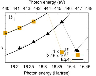
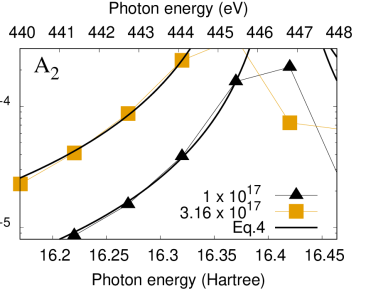
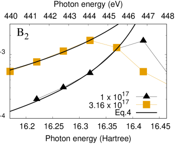
Figure 9: (Color online) Comparison between population transfer calculated with MCTDHF below the Oxygen K-edge, and the three-state second-order formula of Eq. 4, for pulses with intensities 1$\times$10¹⁷ and 3.16$\times$10¹⁷ W cm^-2, as labeled. The fitted intermediate state transition energies are listed in Table 1.

The two maxima for population transfer the A₂ state, which occurred at 447 and 458eV for low intensity in Fig. 7, remain separate as the intensity is increased in Fig. 8, ending up at approximately 445 and 453eV for intensities 3.16$\times$10¹⁷ W cm^-2 and 1.78$\times$10¹⁷ W cm^-2, respectively. The shifts in the maxima for population transfer from 2nd order to the global optima are 2 and 5eV, respectively.

The results in the prior section demonstrated significant higher-order effects at less than 10¹⁶ W cm^-2. The results in this section make clear that even at modest intensity, 10¹⁷ W cm^-2, strong higher-order effects dominate this nominally second-order process. The shifting of the maxima to lower photon energies at higher intensities is probably one of the most straightforward signatures of higher-order effects, being a combination of a 2nd-order AC stark shift with a 2nd-order Raman transition strength for overall fourth-order behavior. The development of the minimum in the valence B₁ population transfer is likely driven by a different above-second-order effect, the direct photoionization of the intermediate core-excited B₁ state which leads to efficient depletion if the pulse is resonant, an overall third-order effect.

The main result is that for all three states, the optimum population transfer is obtained to the $B_{1}$ state with a photon energy significantly 6eV red-detuned from the second-order optimum, 0.70% for the orientation average and 2.39% for an oriented molecule. These optima for population transfer with these 1fs linearly polarized pulses occur at the intensity 3.16$\times$10¹⁷ W cm^-2, and a central frequency of 444eV in our calculations, 6eV red-detuned from the 2nd order optimum at 450eV.

State	Intensity (W cm-2)	Intermediate State Energy (eV)
B1	1 $\times$ 1017	449.28
B1	3.16 $\times$ 1017	449.50
A2	1 $\times$ 1017	446.73
A2	3.16 $\times$ 1017	446.07
B2	1 $\times$ 1017	448.07
B2	3.16 $\times$ 1017	449.82

Table 1: Fit of intermediate state energy $\hbar\omega_{E}$ to three-level second-order perturbation theory expression, Eq. 4, from the fit depicted in Fig. 9.

IX Mechanism of population transfer below edge

The population transfer near the global optimum appears to be driven by nonresonant Raman transitions. At the global optimum population transfer – about 0.8% to the B₁ state, at the intensity 3.16$\times$10¹⁷ W cm^-2, and a central frequency of 444eV – the central frequency of the pulse and the bulk of its 3.25eV bandwidth is substantially red-detuned from the Oxygen K-edge oscillator strength, the near-edge fine structure and the continuum oscillator strength above the edge. In Fig. 8, for each of the three states, the excitation probability drops steeply as the photon energy is decreased going towards the left side of the figures. This strongly decreasing behavior is consistent with nonresonant Raman due to the Oxygen K-edge oscillator strength. In contrast, if population transfer were occurring via direct, resonant, one-electron Raman transitions – via the continuum excitations of the 2$s$ or 2$p$ electron(s) or the 1$s$ electrons of Nitrogen, and not involving the Oxygen 1$s$ – we would expect relatively constant behavior on the left side of the figure.

There is much more integrated oscillator strength available via Oxygen 1s excitations to the the continuum than there is via those to the near-edge fine structure, and therefore nonresonant transitions that are substantially detuned from both the continuum and near-edge fine structure are likely to proceed via the continuum.

However, an analysis of these results for 1fs pulses indicates that the mechanism of population the global optima for population transfer, the data are consistent with a nonresonant Raman transition due to the near-edge fine structure, not the continua. In Fig. 9, we compare the cross section calculated for central frequencies below the Oxygen K-edge with a simple formula based on second-order perturbation theory.

Assuming that the transition is driven by one intermediate electronic state, with transition energy $\hbar\omega_{E}$ from the ground state, the second-order behavior of the population transfer should go approximately as

$$P(\omega_{0})\sim\int d\omega\ \frac{|\mathscr{E}(\omega;\omega_{0})|^{2}|\mathscr{E}(\omega-\Delta;\omega_{0})|^{2}}{(\omega-\omega_{E})^{2}}$$ (4)

in which expression $\Delta$ is the excitation energy corresponding to the Raman transition, and $\mathscr{E}(\omega)$ is the Fourier transfer of the pulse, depending upon central frequency $\omega_{0}$. For a narrow bandwidth, or for large detuning ($\omega_{0}<<\omega_{IE}$), $P(\omega_{0})$ goes as $\frac{1}{\omega_{0}^{2}}$. We approximate the 3.25eV FWHM pulse by a Gaussian, and the Raman transition energy $\Delta$ by the value 3eV.

In Fig. 9, we plot the population transfer results for population transfer below the Oxygen K-edge, and the result of fitting the computed values to Eq. 9. We extract an apparent intermediate state transition energy $\hbar\omega_{E}$ and plot the results in Table 1. The apparent transition energies in Table 1 are near to the positions of the peaks comprising the near-edge fine structure in Fig. 2. Also, the difference between the positions at 1 $\times$ 10¹⁷ W cm^-2 and 3.16 $\times$ 10¹⁷ W cm^-2 are not very large, a fraction of an eV for B₁ and A₂ and 1.75eV for B₂, which would seem to rule out an interpretation relying on AC stark shifts of the continuum oscillator strength. The results therefore support the interpretation that the Raman population transfer near its global optimum for these 1fs linearly polarized pulses is driven by non-resonant electronic Raman transitions via the oscillator strength due to the near-edge fine structure.

X Conclusions

There is good motivation to obtain more complete predictions to guide the development of multidimensional attosecond electronic x-ray Raman spectroscopies Biggs et al. (2012); Mukamel et al. (2013). Considerable effort is being directed currently towards the realization of these methods in the laboratory. X-ray pulses of the required coherence, synchronization, and intensity will soon be available with developments in next-generation light sources or high harmonic generation. It is desirable to provide predictions for the expected efficiencies of these nonlinear methods, which are questionable due to the major direct loss channels (single and multiple ionization) that are unavoidably present. The analogy between these methods and multidimensional nuclear magnetic resonance spectroscopies is tenuous, because the coupling among electrons is so strong.

The theoretical description of the nonlinear quantum dynamics driven in these proposed multidimensional spectroscopic methods requires a coherent representation with many active electrons. Most theoretical and computational treatments so far have not considered the continuum oscillator strength that may alternatively drive the impulsive population transfer process or provide a loss mechanism, and many treatments have been perturbative, explicitly computing only the nth-order response. Calculations that do not consider higher-order effects are incapable of predicting the conditions required to maximize the amplitude of coherent valence excitations created using impulsive electronic Raman transitions in the laboratory.

The MCTHDF method makes it possible to study quantum mechanically coherent nonlinear processes at the limits of intensity without making any assumptions about the degree of excitation, ionization, or correlation of the wave function. Using an implementation of the MCTDHF method that is capable of calculating an accurate solution to the Schrodinger equation including all nonrelativistic electronic effects for polyatomic molecules using current supercomputer technology, we have provided a survey of population transfer to valence electronic states in NO₂ by linearly polarized 1fs pulses tuned near the Oxygen K-edge. The results here for fixed nuclei, averaged over orientations, are expected to closely correspond with the full result including dynamical nuclear motion, due to the short pulse duration and the absence of very light nuclei.

There are omissions in these results that are more questionable than the omission of nuclear motion. Relativistic (broadly speaking, non-dipole) effects are expected to become significant at the highest intensities, and future work will seek to include these effects using a numerically suitable electromagnetic gauge such as that described in Ref. CITE. Furthermore, we have not provided any survey of possible pulse shapes or duration. In future work, we will consider the effect of chirp and duration on the attosecond electronic stimulated Raman population transfer process.

However, we have confirmed the convergence to within ten percent precision for most aspects of these results for population transfer via simulated impulsive electronic x-ray Raman transitions using 1fs linearly polarized pulses, besides those pertaining to the fixed-nuclei nonrelativistic approximations, including the aspects of the one and many-electron representations, and gauge invariance.

Our MCTDHF results indicate that significant (0.70%) population transfer to the lowest $B_{1}$ valence electronic state of the NO₂ molecule may be driven using 1fs x-ray pulses tuned near the Oxygen K-edge. This global optimum for maximum population transfer, orientation-averaged, was found to occur 6eV red-detuned from the 2nd order optimum and 6eV red-detuned from any near-edge fine structure, at 3.16$\times$ 10¹⁷ W cm^-2. Preliminary analysis indicated that it proceeds via nonresonant Raman transitions through the intermediate core-excited metastable states comprising the near-edge fine structure, although more work is required to confirm this explanation.

For an oriented molecule, as the molecule will be for subsequent steps of a multidimensional spectroscopy experiment, the 2.39% population transfer maximum, greatest among the orientations that we calculated, implies a coherence as great as 15%. This degree of coherence would easily enable proposed multidimensional attosecond x-ray spectroscopy experiments. The cleanest experiment would be performed at a lesser intensity, to reduce noise. These calculations indicate that there is no fundamental limitation to the implementation of proposed multidimensional attosecond x-ray spectroscopy methods, based on the efficiency of the population transfer with 1fs pulses.

The main result, optimum population transfer for intense pulses substantially red-detuned below edge, may hold more generally: multidimensional attosecond electronic X-ray Raman spectroscopies might in general most efficiently be performed using intense pulses well red-detuned from resonant edges. Such pulses may minimize loss through direct and sequential ionization and make use of the coherent combination of discrete and continuum edge oscillator strength, thereby providing the greatest potential for creating localized coherent valence electronic wave packets through impulsive stimulated x-ray Raman excitation. Strong red-detuning may provide a way to efficiently perform stimulated Raman transitions, because it prevents an excursion of the 1$s$ electron.

Although the simple fit performed in Sec. IX seemed to indicate that the transition at the global optimum for population transfer is driven by discrete excitation, further work will seek to more fully understand the role of continuum oscillator strength in the population transfer mechanism both at high intensity, near the global optimum, and at lowest order.

Owning the wave function, we may test various hypotheses about the mechanism; MCTDHF allows the problem to be studied without making assumptions about the mechanism beforehand, in a gauge-invariant manner derived from first principles. The MCTDHF method, with its unparalleled variational flexibility and first-principles foundation, may provide answers to questions involving correlated electronic dynamics, and guidance for both models and experiments of the future. Coupled with recent advancements in the greater MCTDHF/MCTDHB/MCTDH effort, such as the entropy-minimzation techniques [CITE] that may improve the convergence, or systems of coupled Lindblad equations [CITE] that may allow the determination of many observables using a small computational domain even with multiple ionization, will increase its power and utility.

It remains to be seen whether the more accurate picture of the nonlinear quantum dynamics driving attosecond stimulated x-ray Raman transitions near their global optimum is that of an excursion of an electron from the 1s shell to the valence space and back, as the Raman process has been modeled so far in terms of solely discrete excitations, or whether the more accurate picture is that of a strongly driven, red-detuned 1$s^{2}$ oscillator, vibrating with both continuum and discrete contributions, that drives the valence transition through electron-electron interaction and Fermi repulsion. In question is whether and how the continuum oscillator strength may combine coherently to drive the population transfer, at lowest order but also as a function of intensity. In question is the range of the excursion of the 1$s$ electron, at lowest order but also as a function of intensity. A greater understanding of the strongly-driven quantum many-body physics that most efficiently drives stimulated x-ray Raman transitions would inform the development of theories and methods specific to multidimensional attosecond x-ray spectroscopy.

XI Acknowledgments

This work was supported by the US Department of Energy Office of Science, Basic Energy Sciences (BES) and Advanced Scientific Computing Research (ASCR) programs, through contracts DE-AC02-05CH11231 and XXXXXXXXXXX, primarily through the US DOE Early Career program. Calculations have been performed on the Lawrencium supercluster at LBNL, administered by the Laboratory Research Computing center, and on the machines of the National Energy Research Scientific Computing Center (NERSC), supported through contracts DE-AC02-05CH11231 and XXXXXXXXXXXXXXXXX. We thank our collaborators in the BigStick project for sharing a large amount computer time, we regret taking so much of it, and we are indebted to the ASCR Leadership Computing Challenge program from which it originated. Further financial support was provided by the Peder Sather Grant program.

References

- Biggs et al. (2012) J. D. Biggs, Y. Zhang, D. Healion, and S. Mukamel, The Journal of Chemical Physics 136, 174117 (2012).
- Mukamel et al. (2013) S. Mukamel, D. Healion, Y. Zhang, and J. D. Biggs, Ann. Rev. Phys. Chem 64, 101 (2013).
- Biggs et al. (2013a) J. D. Biggs, Y. Zhang, D. Healion, and S. Mukamel, The Journal of Chemical Physics 138, 144303 (2013a), http://dx.doi.org/10.1063/1.4799266.
- Biggs et al. (2013b) J. D. Biggs, Y. Zhang, D. Healion, and S. Mukamel, Proceedings of the National Academy of Sciences 110, 15597 (2013b).
- Kirrander et al. (2016) A. Kirrander, K. Saita, and D. V. Shalashilin, Journal of Chemical Theory and Computation 12, 957 (2016), pMID: 26717255, http://dx.doi.org/10.1021/acs.jctc.5b01042 .
- Miyabe and Bucksbaum (2015) S. Miyabe and P. Bucksbaum, Phys. Rev. Lett. 114, 143005 (2015).
- Kitzler et al. (2004) M. Kitzler, J. Zanghellini, C. Jungreuthmayer, M. Smits, A. Scrinzi, and T. Brabec, Phys. Rev. A 70, 041401 (2004).
- Kato and Kono (2004) T. Kato and H. Kono, Chem. Phys. Lett. 392, 533 (2004).
- Caillat et al. (2005) J. Caillat, J. Zanghellini, M. Kitzler, O. Koch, W. Kreuzer, and A. Scrinzi, Phys. Rev. A 71, 012712 (2005).
- Nest et al. (2005) M. Nest, T. Klamroth, and P. Saalfrank, J. Chem. Phys. 122, 124102 (2005).
- Alon et al. (2007) O. E. Alon, A. I. Streltsov, and L. S. Cederbaum, J. Chem. Phys. 127, 154103 (2007).
- Nest et al. (2007) M. Nest, R. Padmanaban, and P. Saalfrank, J. Chem. Phys. 126, 214106 (2007).
- Nest et al. (2008) M. Nest, F. Remacle, and R. D. Levine, New J. Phys. 10, 025019 (2008).
- Kato and Kono (2008) T. Kato and H. Kono, J. Chem. Phys. 128, 184102 (2008).
- Nest (2009) M. Nest, Chem. Phys. Letts. 472, 171 (2009).
- Kato and Yamanouchi (2009) T. Kato and K. Yamanouchi, J. Chem. Phys. 131, 164118 (2009).
- Kato et al. (2009) T. Kato, H. Kono, M. Kanno, Y. Fujimura, and K. Yamanouchi, Laser Physics 19, 1712 (2009).
- Miyagi and Madsen (2013) H. Miyagi and L. B. Madsen, Phys. Rev. A 87, 062511 (2013).
- Sato and Ishikawa (2013) T. Sato and K. L. Ishikawa, Phys. Rev. A 88, 023402 (2013).
- Sato and Ishikawa (2015) T. Sato and K. L. Ishikawa, Phys. Rev. A 91, 023417 (2015).
- Sawada et al. (2016) R. Sawada, T. Sato, and K. L. Ishikawa, Phys. Rev. A 93, 023434 (2016).
- Haxton et al. (2011) D. J. Haxton, K. V. Lawler, and C. W. McCurdy, Phys. Rev. A 83, 063416 (2011).
- Haxton and McCurdy (2015) D. J. Haxton and C. W. McCurdy, Phys. Rev. A 91, 012509 (2015).
- Jones et al. (2016) J. R. Jones, F.-H. Rouet, K. V. Lawler, E. Vecharynski, K. Z. Ibrahim, S. Williams, B. Abeln, C. Yang, W. McCurdy, D. J. Haxton, X. S. Li, and T. N. Rescigno, Molecular Physics 114, 2014 (2016), http://dx.doi.org/10.1080/00268976.2016.1176262 .
- (25) D. J. Haxton, C. W. McCurdy, T. N. Rescigno, K. V. Lawler, J. Jones, B. Abeln, and X. Li, LBNL-AMO-MCTDHF.
- Broeckhove et al. (1988) J. Broeckhove, L. Lathouwers, E. Kesteloot, and P. V. Leuven, Chem. Phys. Lett. 149, 547 (1988).
- Ohta (2004) K. Ohta, Phys. Rev. A 70, 022503 (2004).
- Simon (1979) B. Simon, Physics Letters A 71, 211 (1979).
- Lebedev (1975) V. I. Lebedev, Zh. Vychisl. Mat. mat. Fiz. 15, 48 (1975).
- Lebedev (1976) V. I. Lebedev, Zh. Vychisl. Mat. mat. Fiz. 16, 293 (1976).
- Lebedev (1977) V. I. Lebedev, Sibirsk. Mat. Zh. 18, 132 (1977).
- Lebedev and Skorokhodov (1992) V. I. Lebedev and A. L. Skorokhodov, Dokl. Math 45, 587 (1992).
- Lebedev and Laikov (1999) V. I. Lebedev and D. N. Laikov, Dokl. Math 59, 477 (1999).
- Berkowitz (2002) J. Berkowitz, in Atomic and Molecular Photoabsorption, edited by J. Berkowitz (Academic Press, London, 2002) pp. 237 – 316.
- Jurgensen and Cavell (2000) A. Jurgensen and R. G. Cavell, Chemical Physics 257, 123 (2000).
- Gejo et al. (2003) T. Gejo, Y. Takata, T. Hatsui, M. Nagasono, H. Oji, N. Kosugi, and E. Shigemasa, Chemical Physics 289, 15 (2003), decay Processes in Core-excited Species.
- Piancastelli et al. (2004) M. Piancastelli, V. Carravetta, I. Hjelte, A. D. Fanis, K. Okada, N. Saito, M. Kitajima, H. Tanaka, and K. Ueda, Chemical Physics Letters 399, 426 (2004).