Atomic absorption and emission in non-product states

Abstract

The properties of non-product states, both (anti)symmetrized and entangled, have been extensively studied in the literature. In this paper, by extending previous partial results, we introduce a general framework to describe atomic absorption and emission in these states. Our approach shows the existence of some fundamental differences between entanglement and (anti)symmetrization and between absorption and emission. For instance, modifications of the emission properties with respect to that of uncorrelated systems occur for any (anti)symmetrized state but only for some very specific entangled states.

1 Introduction

Non-product states, entangled and (anti)symmetrized ones, are one of the mainstream topics in physics. Effects associated with the non-factorizable character of the states have been extensively studied, specially violations of Bell’s inequalities, teleportation schemes and applications in quantum cryptography in the case of entangled states, and detection of (anti)bunching and Hong-Ou-Mandel-type interference in the realm of identical particles. Another effects such as the influence of the non-separability on the light-matter interaction and in particular the optical properties of atomic systems, have not deserved so much attention but have led to an independent line of research.

In this line, a review of the influence of entanglement in collective states has been presented in [1], and the possibility of entanglement initiated super Raman scattering in [2]. The modifications on the absorption properties of atoms in (anti)symmetrized states have been described in [3]. A specially relevant work is [4] where, up to our knowledge, the only experimental contribution to the field is considered. The authors measured some emission properties of excited atoms in non-separable states showing that it differs from that of single atoms (in product states). The lifetime of entangled excited atoms has been studied in [5]. The reverse of these phenomena occurs when the atoms are radiated with light in non-factorizable states. Some examples are [6] where two-photon absorption in tapered optical fibers is enhanced, [7] whose authors studied non-linear spectroscopy with entangled photons, and [8] a review of the use of two-mode entangled states to improve the precision of optical metrology. From an even more general perspective, it has been shown the dependence of the light-matter interaction on the separable or non-separable character of the involved states. In particular, it has been demonstrated the modification of the Kapitza-Dirac interference patterns when the state is (anti)symmetrized [9] or entangled (also considering the case of identical particles) [10]. Finally, also related to our work, [11] provides a review of entanglement in atomic systems.

The aim of this paper is to present, based on previous partial results, a general framework to study light absorption and emission by atomic systems in non-product states. Our physical models mimic those used in [3] and [5] and consist of pairs of atoms interacting with light fields. In order to simplify the presentation we shall restrict our considerations to only two atoms. The absorption and emission are described, in a phenomenological way, as transitions between ground and excited states. In this phenomenological model we do not explicitly consider the electromagnetic field. The atoms are in non-product states, either entangled or (anti)symmetrized ones. For entangled states the atoms travel in opposite directions and are well-separated at the time time of interaction with the light. A particular instance of this model is the arrangement in [4], where the photodissociation of molecules leads to pairs of atoms moving in (entangled) almost opposite directions. In contrast, for (anti)symmetrized states, the identical atoms must be close in order to the exchange effects to be important. The arrangements in both cases are very different and will be treated separately. With these models we can determine general expressions for absorption and emission. Moreover, our approach illuminates the differences between entanglement and (anti)symmetrization and between absorption and emission.

2 Entangled states

We study in this section the problem for entangled states. We analyze separately the cases of absorption and emission.

2.1 Absorption

We consider a source of entangled pairs of distinguishable atoms ($A$ and $B$) traveling in opposite directions ($L$ and $R$). The initial state is

$$|\psi_{0}>=\frac{1}{\sqrt{2}}(|A>_{L}|B>_{R}+|B>_{L}|A>_{R})$$ (1)

When they are well-separated we introduce an interaction with a light beam placed at $L$. We use a broad band frequency beam that includes absorption frequencies for the two atoms. The light intensity is low enough to discard double absorptions. This procedure is equivalent to radiate simultaneously with two beams sharped around the excitation frequencies of the two atoms.

A possible realization of this source is the dissociation of diatomic molecules composed of two different isotopes of the same species. The isotopes approximately match the above resonant condition for the incident light. This source is reminiscent of the arrangement in [4], although in that case the two dissociated atoms are identical and are in excited states.

After the interaction with the light the atoms evolve as $|A>_{L}\rightarrow\alpha|A^{*}>_{L}+\beta|A>_{L}$ and $|B>_{L}\rightarrow\gamma|B^{*}>_{L}+\delta|B>_{L}$ with $A^{*}$ and $B^{*}$ denoting the excited states of the atoms. The coefficients obey the normalization conditions $|\alpha|^{2}+|\beta|^{2}=1$ and $|\gamma|^{2}+|\delta|^{2}=1$. In order to avoid double absorptions we must have $|\alpha_{i}|^{2}\ll 1$ and $|\gamma_{i}|^{2}\ll 1$. The state after the interaction is

$$|\psi_{i}>=\frac{1}{\sqrt{2}}(\alpha_{L}|A^{*}>_{L}|B>_{R}+\beta_{L}|A>_{L}|B>_{R}+$$

$$\gamma_{L}|B^{*}>_{L}|A>_{R}+\delta_{L}|B>_{L}|A>_{R})$$ (2)

The probability amplitudes of absorption by the atoms $A$ and $B$ are respectively $\alpha_{L}/\sqrt{2}$ and $\gamma_{L}/\sqrt{2}$. The total probability of absorption in the state $\psi_{i}$ is obtained by adding both probability amplitudes. In effect, the two absorption alternatives (to be absorbed by atom $A$ or by atom $B$) are indistinguishable as long as both are compatible with the broad band range of the beam. The total one-absorption probability is

$$P_{one}=\frac{1}{2}|\alpha_{L}+\gamma_{L}|^{2}=\frac{1}{2}|\alpha_{L}|^{2}+\frac{1}{2}|\gamma_{L}|^{2}+Re(\alpha_{L}^{*}\gamma_{L})$$ (3)

It must be compared with that associated with a mixture of the product states $|A>_{L}|B>_{R}$ and $|B>_{L}|A>_{R}$ with equal weights ($1/2$), which is $P_{one}^{mix}=(|\alpha_{L}|^{2}+|\gamma_{L}|^{2})/2$. Both expressions differ by the interference term $Re(\alpha_{L}^{*}\gamma_{L})$. It represents the interference effect associated with the presence of indistinguishable absorption alternatives. Entanglement modifies the absorption properties of the pair of atoms.

At this point we must specify the observables associated with the measurement of the absorption probability. In the one-particle case that operator is the projector on state $A^{*}$, $\hat{\theta}_{A}=|A^{*}><A^{*}|$, which acts as $\hat{\theta}_{A}|A^{*}>=|A^{*}>$ and $\hat{\theta}_{A}|A>=0$, giving the eigenvalues $1$ and $0$ corresponding to excited and non-excited states. In the two-particle case the operators are $\hat{O}_{A}=\hat{\theta}_{A}\otimes\hat{1}$ and $\hat{O}_{B}=\hat{\theta}_{B}\otimes\hat{1}$, acting $\hat{\theta}$ on the left side and $\hat{1}$ on the right one. We have $\hat{O}_{A}|A^{*}>_{L}|B>_{R}=|A^{*}>_{L}|B>_{R},\cdots$. The observable for the measurement of excited states at $L$ (independently of being of type $A$ or $B$) is $\hat{O}_{A}+\hat{O}_{B}$. We would obtain the same results using the non-local observable $\hat{O}=\hat{\theta}_{A}\otimes|B>_{R}<B|+\hat{\theta}_{B}\otimes|A>_{R}<A|$ (which is the projector over the subspaces of excited states at $L$ and non-excited ones at $R$). However, for the type of state and interaction used in the paper the non-local observable would be redundant from the local one. For instance, as at $R$ we must have an atom of type $B$ if at $L$ there is one of type $A$ and the interaction takes place at $L$, $|B>_{R}<B|$ in $\hat{O}$ is equivalent to $\hat{1}$ in $\hat{O}_{A}+\hat{O}_{B}$. The fact that the observable must be local can be seen from a possible experimental realization of the measurement. We place photon detectors at $L$, corresponding each detection event to the spontaneous emission by an excited atom. There is not need for a measurement process at $R$. In a more abstract form, the full two-particle state reduces when the measurement at $L$ is performed, being not necessary a measurement device at $R$. This is a fundamental property of entangled states. There is a non-local aspect in the measurement process, but it is related to the state not to the observable.

To end the subsection we remark that this scheme is only valid for distinguishable atoms. When the atoms are identical the initial state reads as $|A>_{L}|A>_{R}$ that is not an entangled state but a product one. As we shall see later, the absorption properties of pairs of identical atoms can be modified, but due to (anti)symmetrization.

2.2 Emission

Let us consider a pair of atoms in the excited entangled state

$$|\psi_{exc}>=\frac{1}{\sqrt{2}}(|A^{*}>_{L}|B>_{R}+|B^{*}>_{L}|A>_{R})$$ (4)

This state can be prepared, for instance, using the dissociation of diatomic molecules with one of the atoms in an excited state. As in subsection 2.1 this source closely remembers the arrangement described in [4].

The excited atoms spontaneously emit photons. We could expect entanglement-based effects on the emission probabilities similar to those found for absorption. However, the conditions for the existence of these effects are now much more stringent. In effect, the emission probabilities will give rise to interference effects and consequently will differ from those of mixtures of product states only when the photon emission is compatible with the two alternatives (emission by $|A^{*}>_{L}|B>_{R}$ or by $|B^{*}>_{L}|A>_{R}$). In general, different atoms have different emission frequencies, becoming distinguishable the two alternatives. The two alternatives are only indistinguishable in very particular circumstances, for instance, when the emission frequencies are very close and cannot be distinguished because of the radiative broadening. The simplest realization of the scheme would be based on the use of two different isotopes of the same species.

We evaluate the emission probability when the two alternatives are indistinguishable. The description of the previous subsection is not adequate for our problem because, for large times, all the excited atoms decay to the ground state. We must instead consider emission probabilities at a given time, that is, a time-dependent formalism. Consequently a description based on the evolution operator $\hat{U}$ is more adequate for the problem. As after the preparation there is not interaction between the atoms the evolution operator factorizes, $\hat{U}=\hat{U}_{A}\hat{U}_{B}$. In the final state after emission the two atoms are in the ground state and consequently, $|\psi_{f}>=|\psi_{0}>$. Note that after the emission, as we have assumed the photon to be compatible with the two alternatives, the superposition is not broken and the state remains a pure one instead of becoming a mixture. The matrix element for the emission transition is ${\cal M}_{em}(t)=<\psi_{f}|\hat{U}(t)|\psi_{exc}>$. The emission probability at time $t$, $P_{em}(t)=|{\cal M}_{em}(t)|^{2}$, can be written as

$$P_{em}(t)=\frac{1}{4}|{\cal M}_{A}^{s}(t){\cal M}_{B,nt}^{s}(t)|^{2}+\frac{1}{4}|{\cal M}_{B}^{s}(t){\cal M}_{A,nt}^{s}(t)|^{2}+$$

$$\frac{1}{2}Re({\cal M}_{A}^{s*}(t){\cal M}_{B,nt}^{s*}(t){\cal M}_{B}^{s}(t){\cal M}_{A,nt}^{s}(t))=\frac{1}{4}P_{A}^{s}(t)|{\cal M}_{B,nt}^{s}(t)|^{2}+$$

$$\frac{1}{4}P_{B}^{s}(t)|{\cal M}_{A,nt}^{s}(t)|^{2}+\frac{1}{2}Re({\cal M}_{A}^{s*}(t){\cal M}_{B,nt}^{s*}(t){\cal M}_{B}^{s}(t){\cal M}_{A,nt}^{s}(t))$$ (5)

with ${}_{L}<A|\hat{U}_{A}|A^{*}>_{L}={\cal M}_{A}^{s}$ and ${}_{L}<B|\hat{U}_{B}|B^{*}>_{L}={\cal M}_{B}^{s}$ the single-atom emission matrix elements for $A$ and $B$. Their squared modulus are the single-atom emission probabilities. On the other hand, ${\cal M}_{A,nt}^{s}=_{R}<A|\hat{U}_{A}|A>_{R}$ and ${\cal M}_{B,nt}^{s}=_{R}<B|\hat{U}_{B}|B>_{R}$ are the non-transition matrix elements, which only depend on the center of mass (CM) evolution of the state. To derive the above equation we have used the fact that the terms ${}_{L}<A|_{R}<B|\hat{U}|B^{*}>_{L}|A>_{R}$ and ${}_{L}<B|_{R}<A|\hat{U}|A^{*}>_{L}|B>_{R}$ vanish.

This result must be compared with that for a mixture of initial product states $|A^{*}>_{L}|B>_{R}$ and $|B^{*}>_{L}|A>_{R}$ with equal weights, given by $P_{em}^{mix}(t)=(P_{A}^{s}(t)|{\cal M}_{B,nt}^{s}(t)|^{2}+P_{B}^{s}(t)|{\cal M}_{A,nt}^{s}(t)|^{2})/2$. We have again interference effects between the two alternatives that lead to a modification of the emission properties due to entanglement. We remark again that for this scheme the effects only occur when the emission alternatives are indistinguishable.

We represent graphically the above results. In the standard description of spontaneous emission the total probability of emission between the preparation of the state ($t=0$) and time $t$ is $P_{A}^{s}(t)=1-e^{-t/\tau_{A}}$ with $\tau_{A}$ the lifetime of atom $A$. The matrix element can be expressed as ${\cal M}_{A}^{s}=M_{A}^{s}<\psi_{A}|\hat{U}_{spa}(t)|\psi_{A^{*}}>$, with $M_{A}^{s}$ the matrix element of the internal variables which must have the form $M_{A}^{s}=(1-e^{-t/\tau_{A}})^{1/2}$ up to a phase factor, the $\psi$’s the wave functions representing the spatial part of the states and $\hat{U}_{spa}$ the spatial part of $\hat{U}$. $<\psi_{A}|\hat{U}_{spa}(t)|\psi_{A}^{*}>$ is the scalar product of the evolved excited state and the non-excited one. If we assume that the recoil associated with the emission and the spreading of the wave function during the free evolution are small we have $<\psi_{A}|\hat{U}_{spa}(t)|\psi_{A^{*}}>\approx 1$ and we can take ${\cal M}_{A}^{s}\approx M_{A}^{s}=(1-e^{-t/\tau_{A}})^{1/2}$. Similarly, as we assume the spreading small we have ${\cal M}_{A,nt}^{s}\approx 1$. With all these expressions, taking $\tau_{A}=1$ as the time unit and $\tau_{B}=0.1$ we obtain the curves in Fig. 1. We see that at short times the probability of emission is larger for product states.

Figure 1: Dependence of the emission probability on time (in units of the lifetime of atom $A$). The continuous line represents entangled states and the dashed one a mixture of product ones.

3 (Anti)symmetrized states

In this section we analyze the same problem for (anti)symmetrized states of identical particles. The case of absorption has already been considered in [3]. Here we shall extend that study to the general case by discarding a simplification used there. Later, we shall study emission.

A difference with the case of entangled states is that now, in addition to the internal variables, we must explicitly introduce into the formalism the CM-ones. In the calculations in the previous section the CM-wave function only played a role similar to that of the subscripts $L$ and $R$ labeling the alternatives. In contrast, when the particles are identical the CM-wave functions determine the overlapping of the two particles. The overlapping, defined as the scalar product of the two wave functions, measures if the two wave function domains lie in the same spatial region or in different ones. Only in the first case the exchange effects are important. The CM-wave functions must be included in all the steps of the calculations as they even determine the normalization factors.

3.1 Absorption

We use the same notation introduced in [3]. The initial state of the pair of identical atoms before the interaction with the light is

$$|\Psi_{i}>=N_{i}(|\phi_{g}>_{1}|\psi_{g}>_{2}\pm|\psi_{g}>_{1}|\phi_{g}>_{2})$$ (6)

with the normalization factor $N_{i}=(2(1\pm|<\phi|\psi>|^{2}))^{-1/2}$. The state $|\psi_{g}>=|\psi>|g>$ is the product of the CM-wave function and the internal state, denoting $g$ the ground state. The upper sign in the double sign expressions refers to bosons and the lower one to fermions.

When an atom absorbs a photon its state changes: $|\psi_{g}>\rightarrow|\tilde{\psi}_{e}>$ and $|\phi_{g}>\rightarrow|\tilde{\phi}_{e}>$, denoting $|e>$ the internal excited state. Because of the recoil the CM-wave function changes to $\tilde{\psi}$ or $\tilde{\phi}$. There are two alternatives for the absorption depending on which atomic state the photon has been absorbed. These alternatives are represented by the states:

$$|\Psi_{abs}(\tilde{\psi})>=N_{abs}(\tilde{\psi})(|\tilde{\psi}_{e}>_{1}|\phi_{g}>_{2}\pm|\phi_{g}>_{1}|\tilde{\psi}_{e}>_{2})$$ (7)

and

$$|\Psi_{abs}(\tilde{\phi})>=N_{abs}(\tilde{\phi})(|\tilde{\phi}_{e}>_{1}|\psi_{g}>_{2}\pm|\psi_{g}>_{1}|\tilde{\phi}_{e}>_{2})$$ (8)

with the normalization factor $N_{abs}(\tilde{\psi})=(2(1\pm|<\phi|\tilde{\psi}>|^{2}))^{-1/2}$. A similar expression holds for $N_{abs}(\tilde{\phi})$. Note that, at variance with Eqs. (3) and (4) of [3], the normalization factors of Eqs. (7) and (8) are not $1/\sqrt{2}$ but depend on the overlapping. This difference is due to the fact that in [3] it was assumed a small overlapping, equivalent to the assumption of a large recoil, $|<\phi|\tilde{\psi}>|^{2}\ll 1$ and $|<\psi|\tilde{\phi}>|^{2}\ll 1$.

In [3], in order to simplify the presentation, it was also assumed that the final state after the absorption was a mixture. This again corresponds to small overlapping. We do not longer rely on this assumption and consequently we move to the general case. The consequence of this extension is that now the two alternatives are indistinguishable: as the overlapping is no longer negligible we cannot distinguish if the photon was absorbed by the particle in state $\psi$ or by that in $\phi$. We must add the probability amplitudes. This is equivalent to consider a final pure state of the system after the absorption, $|\Psi_{f}>=N_{f}(|\Psi_{abs}(\tilde{\psi})>+|\Psi_{abs}(\tilde{\phi})>)$, with $N_{f}=(2+2Re(<\Psi_{abs}(\tilde{\psi})|\Psi_{abs}(\tilde{\phi})>))^{-1/2}$ and $<\Psi_{abs}(\tilde{\psi})|\Psi_{abs}(\tilde{\phi})>=2N_{abs}(\tilde{\psi})N_{abs}(\tilde{\phi})<\tilde{\psi}|\tilde{\phi}><\phi|\psi>$, where we have used $<e|g>=0$.

The one-absorption probability is $P_{one}^{ide}=|<\Psi_{f}|\hat{U}|\Psi_{i}>|^{2}=N_{f}^{2}|{\cal M}_{\tilde{\psi}}+{\cal M}_{\tilde{\phi}}|^{2}$ with the superscript $ide$ in the probability denoting that now we are dealing with identical particles and ${\cal M}_{\tilde{\psi}}=<\Psi_{abs}(\tilde{\psi})|\hat{U}|\Psi_{i}>$. We fix the time $t$ at which the magnitudes are evaluated and we do not longer include it explicitly into the equations. Assuming again that there is no interaction between the atoms the evolution operator factorizes, $\hat{U}=\hat{U}_{1}\hat{U}_{2}\equiv\hat{U}_{s}\hat{U}_{s}$, with $\hat{U}_{s}$ denoting the single-particle operator. Using this property it is simple to obtain ${\cal M}_{\tilde{\psi}}=2N_{abs}(\tilde{\psi})N_{i}({\cal M}_{\tilde{\psi}\phi}^{s}{\cal M}_{\phi\psi}^{s}\pm{\cal M}_{\tilde{\psi}\psi}^{s}{\cal M}_{\phi\phi}^{s})$ for the first alternative and ${\cal M}_{\tilde{\phi}}=2N_{abs}(\tilde{\phi})N_{i}({\cal M}_{\tilde{\phi}\phi}^{s}{\cal M}_{\psi\psi}^{s}\pm{\cal M}_{\tilde{\phi}\psi}^{s}{\cal M}_{\psi\phi}^{s})$ for the second one, denoting ${\cal M}_{\tilde{\psi}\phi}^{s}=<\tilde{\psi}_{e}|\hat{U}_{s}|\phi_{g}>$, . .. the single-particle matrix elements.

From the above equations it is possible to analyze the mathematical structure of the absorption probabilities. There are three physical factors that determine the form of the probabilities: the overlapping of the CM-wave functions present in the normalization coefficients, the indistinguishability of the absorption alternatives ruling the addition of probability amplitudes, and the (anti)symmetrized character of the wave function. The last two factors give rise to interference effects. To study its form it is convenient to express the two-particle matrix elements as ${\cal M}_{\tilde{\psi}}={\cal M}_{\tilde{\psi}}^{d}\pm{\cal M}_{\tilde{\psi}}^{e}$,.. denoting the superscripts $d$ and $e$ the direct and exchange terms. With this notation the absorption probability reads

$$P_{one}^{ide}/N_{f}^{2}=|{\cal M}_{\tilde{\phi}}^{d}|^{2}+|{\cal M}_{\tilde{\phi}}^{e}|^{2}\pm 2Re({\cal M}_{\tilde{\phi}}^{d*}{\cal M}_{\tilde{\phi}}^{e})+|{\cal M}_{\tilde{\psi}}^{d}|^{2}+|{\cal M}_{\tilde{\psi}}^{e}|^{2}\pm$$

$$2Re({\cal M}_{\tilde{\psi}}^{d*}{\cal M}_{\tilde{\psi}}^{e})+2Re({\cal M}_{\tilde{\phi}}^{d*}{\cal M}_{\tilde{\psi}}^{d}\pm{\cal M}_{\tilde{\phi}}^{d*}{\cal M}_{\tilde{\psi}}^{e}\pm{\cal M}_{\tilde{\phi}}^{e*}{\cal M}_{\tilde{\psi}}^{d}+{\cal M}_{\tilde{\phi}}^{e*}{\cal M}_{\tilde{\psi}}^{e})$$ (9)

The four squared modulus terms represent the probabilities associated with the four absorption alternatives available to the system: $(\phi_{g}\rightarrow\tilde{\psi}_{e};\psi_{g}\rightarrow\phi_{g})$, $(\psi_{g}\rightarrow\tilde{\psi}_{e};\phi_{g}\rightarrow\phi_{g})$, $(\psi_{g}\rightarrow\tilde{\phi}_{e};\phi_{g}\rightarrow\psi_{g})$ and $(\phi_{g}\rightarrow\tilde{\phi}_{e};\psi_{g}\rightarrow\psi_{g})$, corresponding respectively to ${\cal M}_{\tilde{\psi}}^{d},{\cal M}_{\tilde{\psi}}^{e},{\cal M}_{\tilde{\phi}}^{d}$ and ${\cal M}_{\tilde{\phi}}^{e}$.

The other terms correspond to the six interference effects existent between these four alternatives. We must distinguish between three different types of interference effects: exchange, indistiguishability and mixed ones. The two exchange terms (${\cal M}_{\tilde{\phi}}^{d*}{\cal M}_{\tilde{\phi}}^{e}$ and ${\cal M}_{\tilde{\psi}}^{d*}{\cal M}_{\tilde{\psi}}^{e}$) emerge directly from the superposition of direct and exchange terms with the same final states ($\tilde{\phi}_{e},\psi_{g}$ and $\tilde{\psi}_{e},\phi_{g}$). They differ for bosons and fermions via the characteristic double sign $\pm$. On the other hand, the indistinguishability terms (${\cal M}_{\tilde{\phi}}^{d*}{\cal M}_{\tilde{\psi}}^{d}$ and ${\cal M}_{\tilde{\phi}}^{e*}{\cal M}_{\tilde{\psi}}^{e}$) are equal for bosons and fermions and their matrix element products only contain direct or exchange terms. Their physical origin is the existence of indistinguishable alternatives (final states $\tilde{\phi}_{e},\psi_{g}$ and $\tilde{\psi}_{e},\phi_{g}$ after the absorption). Finally, the mixed terms (${\cal M}_{\tilde{\phi}}^{d*}{\cal M}_{\tilde{\psi}}^{e}$ and ${\cal M}_{\tilde{\phi}}^{e*}{\cal M}_{\tilde{\psi}}^{d}$) share characteristics with the previous ones. They contain direct and exchange matrix elements reflecting an exchange-type contribution, but at the same time they refer to different final states, a typical property of indistinguishability-type terms. Then both types of physical effects are present in the mixed terms. In particular, they differ for bosons and fermions.

We represent graphically the absorption probabilities. As discussed for Fig. 1 the matrix elements ${\cal M}_{\tilde{\psi}\phi}^{s}$ represent the product of the internal matrix element and the overlapping of $\tilde{\psi}$ and the evolved $\phi(t)$. We assume again that the recoil of the atom by the absorption is small and that the spreading of $\phi$ during the free evolution is not too large (taking for $t$ small values after the atom-light interaction). Then we can approximate the spatial part of ${\cal M}_{\tilde{\psi}\phi}^{s}$ by the time-independent overlapping $<\tilde{\psi}|\phi>$. We take for the internal matrix element $M^{s}=1$ and represent the absorption probability versus the initial overlapping $<\psi|\phi>$. We use for the other overlapping parameters the values $<\tilde{\psi}|\tilde{\phi}>=0.5$ and $0.9$, $<\tilde{\psi}|\phi>=0.6=<\tilde{\phi}|\phi>$, $<\psi|\tilde{\phi}>=<\psi|\phi><\tilde{\psi}|\phi>$ and $<\tilde{\psi}|\psi>=<\psi|\phi><\tilde{\psi}|\phi>$ (choice equivalent to fix $\phi$,$\tilde{\phi}$ and $\tilde{\psi}$ and to vary $\psi$).

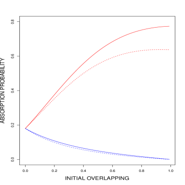
Figure 2: Variation of the absorption probability with respect to the initial overlapping. The red and blue curves correspond respectively to bosons and fermions, and the continuous and discontinuous ones to the values $0.5$ and $0.9$ of $<\tilde{\psi}|\tilde{\phi}>$.

The results are presented in Fig. 2. For zero initial overlapping we have the absorption probability of distinguishable particles. When that overlapping increases we observe deviations from the distinguishable behavior. The probabilities for fermions are always smaller. In particular, when the initial overlapping tends to one the probability vanish, reflecting the Pauli exclusion principle. In contrast, for bosons the probabilities always increase with respect to the values of non-identical particles. The variation between the curves for different values of $<\tilde{\psi}|\tilde{\phi}>$ is much larger in the case of bosons.

3.2 Emission

We consider now emission by excited states of identical particles. For the sake of concreteness we only consider the case with the two atoms initially excited. This is the most interesting case because it is closely related to the experimental arrangement in [4], where the photodissociation of a $H_{2}$ molecule leads to two excited Hydrogen atoms. The initial state is

$$|\Psi_{exc}>=N_{i}(|\phi_{e}>_{1}|\psi_{e}>_{2}\pm|\psi_{e}>_{1}|\phi_{e}>_{2})$$ (10)

We want to evaluate the probability of double emission after a fixed time that, as signaled before, is not explicitly included in the equations. Note that the direction of photon emission is random and varies from repetition to repetition of the experiment. After the emission the atom suffers a recoil and its CM-wave function also changes in a random way. We make the evaluation for only two fixed emission directions, which correspond to the final state

$$|\Psi_{F}(\overline{\phi},\overline{\psi})>=N_{F}(\overline{\phi},\overline{\psi})(|\overline{\phi}_{g}>_{1}|\overline{\psi}_{g}>_{2}\pm|\overline{\psi}_{g}>_{1}|\overline{\phi}_{g}>_{2})$$ (11)

with $N_{F}(\overline{\phi},\overline{\psi})=(2(1\pm|<\overline{\phi}|\overline{\psi}>|^{2}))^{-1/2}$. Note that as the emission processes are indistinguishable (the particles are identical) the final state is a pure one. This property agrees with the fact that the final state of the atom-photon system after emission is a pure entangled one [12, 13]. In our case, as the light field variables are not explicitly included, the total atom-photon pure state can be expressed in the form $\Psi_{F}(\overline{\phi},\overline{\psi})$.

The probability amplitude for the transition is $<\Psi_{F}(\overline{\phi},\overline{\psi})|\hat{U}|\Psi_{exc}>$, and the probability can be written as

$$P_{two}^{ide}=\frac{P_{\overline{\phi}\phi}^{s}P_{\overline{\psi}\psi}^{s}+P_{\overline{\phi}\psi}^{s}P_{\overline{\psi}\phi}^{s}\pm 2Re({\cal M}_{\overline{\phi}\phi}^{s*}{\cal M}_{\overline{\psi}\psi}^{s*}{\cal M}_{\overline{\phi}\psi}^{s}{\cal M}_{\overline{\psi}\phi}^{s})}{(1\pm|<\phi|\psi>|^{2})(1\pm|<\overline{\phi}|\overline{\psi}>|^{2})}$$ (12)

where, as in the previous section, $P_{\overline{\phi}\phi}^{s}=|{\cal M}_{\overline{\phi}\phi}^{s}|^{2}$ and ${\cal M}_{\overline{\phi}\phi}^{s}=<\overline{\phi}_{g}|\hat{U}_{s}|\phi_{e}>$.

From this equation we see that the emission probability depends on the overlapping between both the initial ($<\phi|\psi>$) and the final ($<\overline{\phi}|\overline{\psi}>$) CM-wave functions and on the exchange interference between the two available alternatives, $(\phi_{e}\rightarrow\overline{\phi}_{g};\psi_{e}\rightarrow\overline{\psi}_{g})$ and $(\psi_{e}\rightarrow\overline{\phi}_{g};\phi_{e}\rightarrow\overline{\psi}_{g})$.

4 Discussion

We have analyzed the absorption and emission processes in non-product atomic states in two archetypical situations that represent a rather general framework for the problem. The fundamental characteristics of most arrangements can be described via these situations with minor changes. Some properties of these processes in non-factorizable states have been previously presented in the literature but in a somewhat disperse way. We consider useful the unified view introduced here.

The most important consequence of our analysis is to show that the absorption and emission probabilities in non-factorizable atomic states differ in many cases with respect to those of product states. This property can be seen as a distinctive characteristic of non-product states, just as violations of Bell’s inequalities, (anti)bunching,… These differences have a rich and diverse structure. The most extreme case is that of absorption in (anti)symmetrized states, where four types of modifications are present: dependence on the overlapping and three types of interferences, by exchange effects, by the existence of indistinguishable alternatives and by the joint action of the two previous causes.

In addition to provide a general framework for the problem, our approach illustrates some aspects of the subject that deserve attention. The first one is the relation between entanglement and (anti)symmetrization. There is some controversy in the literature about this point. Some times they are considered as rather similar concepts because both represent multi-particle superpositions. As a matter of fact, from a mathematical point of view, they are described by the same type of non-factorizable equation (with the important difference of the normalization coefficient). However, there are some fundamental differences between both types of superpositions. The first one, and most evident, is that exchange effects only occur when the particles are very close whereas entanglement-based effects can be present at large separations (as in the arrangement here considered). This property is closely related to the different role of the CM-wave function in both cases. For identical particles it determines the strength of the exchange effects and its scalar product enters into the normalization factor. In contrast, for entangled systems it plays a secondary role equivalent to that of the labels that denote if one particle goes to the left or to the right. In this paper we have shown another important difference: (anti)symmetrization modifies the emission properties for any excited state of the multi-particle system (even with the atoms in different excited states) whereas entanglement can only do it when the emission alternatives are indistinguishable. For identical particles it is an universal property and for entangled ones almost an exception.

All the considerations in this paper about identical particles refer to states without entanglement, that is, the non-separability in the system is exclusively associated with the (anti)symmetrization. A natural further step is to study identical particles in entangled states (see [11] for a general view and [10, 14, 15, 16] for particular considerations). This is an interesting and controversial field. In particular, with reference to the fundamental role played by the overlapping in systems of identical particles, the authors of [14] have analyzed not only the overlapping of the states (as we have done here), but also how the overlapping evolves during the process of interaction with the detectors, quantifying the mutual dependence between measurement processes and effective particle distinguishability. On the other hand, in [15] a more general framework for the problem, based on the quantumness of correlations, has been introduced. Finally, in [16] entanglement measures for fermionic systems with not fixed particle number have been discussed.

Another point illustrated by our analysis refers to the differences between absorption and emission. As discussed before the emission properties are radically different for (anti)symmetrized and entangled states, whereas such a sharp contrast is not present for absorption. Another manifestation only concerning to entangled states, is that in the presence of entanglement the absorption rates are modified with respect to those of product states, in marked contrast with emission where the process only occurs when the emission alternatives are indistinguishable. The modification of the absorption properties is a much more general phenomenon than in the case of emission.

References

- [1] Z. Ficek, R. Tanaś, Phys. Rep. 372, 369 (2002)
- [2] G. S. Agarwal, Phys. Rev. A 83, 023802 (2011)
- [3] P. Sancho, Ann. Phys. 336, 482 (2013)
- [4] T. Tanabe, T. Odagiri, M. Nakano, Y. Kumagai, I. H. Suzuki, M. Kitajima, N. Kouchi, Phys. Rev. A 82, 040101(R) (2010)
- [5] P. Sancho, L. Plaja, J. Phys. B 42, 165008 (2009)
- [6] H. You, S. M. Hendrickson, J. D. Franson, Phys. Rev. A 78, 053803 (2008)
- [7] O. Roslyak, C. A. Mark, S. Mukame, Phys. Rev. A 79, 033832 (2009)
- [8] J. P. Dowling, Contem. Phys. 49, 125 (2008)
- [9] P. Sancho, Phys. Rev. A 82, 033814 (2010)
- [10] P. Sancho, Ann. Phys. 355, 143 (2015)
- [11] M. C. Tichy, F. Mintert, A. Buchleitner, J. Phys. B 44, 192001 (2011)
- [12] V. Weisskopf, E. Wigner, Z. Phys. 63, 54 (1930)
- [13] K. Rzazewski, W. Zackowicz, J. Phys. B 25, L319 (1992)
- [14] M. C. Tichy, F. de Melo, M. Kuś, F. Mintert, A. Buchleitner, Fortschr. Phys. 61, 225 (2013)
- [15] F. Iemini, T. Debarba, R. O. Vianna, Phys. Rev. A 89, 032324 (2014)
- [16] N. Gigena, R. Rossignoli, Phys. Rev. A 92, 042326 (2015)