Information Theoretic Structure Learning with Confidence

Abstract

Information theoretic measures (e.g. the Kullback Liebler divergence and Shannon mutual information) have been used for exploring possibly nonlinear multivariate dependencies in high dimension. If these dependencies are assumed to follow a Markov factor graph model, this exploration process is called structure discovery. For discrete-valued samples, estimates of the information divergence over the parametric class of multinomial models lead to structure discovery methods whose mean squared error achieves parametric convergence rates as the sample size grows. However, a naive application of this method to continuous nonparametric multivariate models converges much more slowly. In this paper we introduce a new method for nonparametric structure discovery that uses weighted ensemble divergence estimators that achieve parametric convergence rates and obey an asymptotic central limit theorem that facilitates hypothesis testing and other types of statistical validation.

Index Terms—  mutual information, structure learning, ensemble estimation, hypothesis testing

1 Introduction

Information theoretic measures such as mutual information (MI) can be applied to measure the strength of multivariate dependencies between random variables (RV). Such measures are used in many applications including determining channel capacity [1], image registration [2], independent subspace analysis [3], and independent component analysis [4]. MI has also been used for structure learning in graphical models (GM) [5], which are factorizable multivariate distributions that are Markovian according to a graph [6]. GMs have been used in fields such as bioinformatics, image processing, control theory, social science, and marketing analysis. However, structure learning for GMs remains an open challenge since the most general case requires a combinatorial search over the space of all possible structures [7, 8] and nonparametric approaches have poor convergence rates as the number of samples increases. This prevents reliable application of nonparametric structure learning except for impractically large sample sizes. This paper proposes a nonparametric MI-based ensemble estimator for structure learning that achieves the parametric mean squared error (MSE) rate when the densities are sufficiently smooth and admits a central limit theorem (CLT) which enables us to perform hypothesis testing. We demonstrate this estimator in multiple structure learning experiments.

Several structure learning algorithms have been proposed for parametric GMs including discrete Markov random fields [9], Gaussian GMs [10], and Bayesian networks [11]. Recently, the authors of [12] proposed learning latent variable models from observed samples by estimating dependencies between observed and hidden variables. Numerous other works have demonstrated that latent tree models can be learned efficiently in high dimensions (e.g. [13, 14]).

We focus on two methods of nonparametric structure learning based on ensemble MI estimation. The first method is the Chow-Liu (CL) algorithm which constructs a first order tree from the MI of all pairs of RVs to approximate the joint pdf [5]. Since structure learning approaches can suffer from performance degradation when the model does not match the true distribution, we propose hypothesis testing via MI estimation to determine how well the tree structure imposed by the CL algorithm approximates the joint distribution. The second method learns the structure by performing hypothesis testing on the MI of all pairs of RVs. An edge is assigned between two RVs if the MI is statistically different from zero.

Accurate MI estimation is necessary for both methods. Estimating MI is often difficult, especially in high dimensions when there is no parametric model for the data. Nonparametric methods of estimating MI have been proposed including $k$-nearest neighbor based methods [15, 16] and minimal spanning trees [17]. However, the MSE convergence rates of the latter estimator are currently unknown, while the $k$-nn based methods achieve the parametric rate only when the dimension of each of the RVs is less than 3 [18].

Recent work has focused on the more general problem of nonparametric divergence estimation including approaches based on optimal kernel density estimators (KDE) [19, 20, 21] and ensemble methods [22, 23, 24, 25]. While the optimal KDE-based approaches can achieve the parametric MSE rate for smooth densities (i.e. the densities are at least $d$ [20] or $d/2$ [19, 21] times differentiable where $d$ is the dimension of the data), they can be difficult to construct near the density support boundary and they require knowledge of the boundary. Also, for some types of divergence functionals, these approaches require numerical integration which requires many computations.

In contrast, the ensemble estimators in [23, 24, 25, 22] vary the neighborhood size of nonparametric density estimators to construct an ensemble of simple plug-in divergence or entropy estimators. The final estimator is a weighted average of the ensemble of estimators where the weights are chosen to decrease the bias with only a small increase in the variance. Specifically, the ensemble estimator in [25] achieves the parametric MSE rate without any knowledge of the densities’ support set when the densities are $(d+1)/2$ times differentiable.

2 Factor Graph Learning

This paper focuses on learning a second-order product approximation (i.e. a dependence tree) of the joint probability distribution of the data. Let $\mathbf{X}^{(i)}$ denote the $i$th component of a $d$-dimensional random vector $\mathbf{X}$. We use similar notation to [5] where the goal is to approximate the joint probability density $p(\mathbf{X})$ as

$$p^{\prime}\left(\mathbf{X}\right)=\prod_{i=1}^{d}p\left(\mathbf{X}^{(m_{i})}|\mathbf{X}^{(m_{j(i)})}\right),$$ (1)

where $0\leq j(i)<i,$ $\left(m_{1},\dots,m_{d}\right)$ is a (unknown) permutation of $1,\,2,\,\dots d$, $p\left(\mathbf{X}^{(i)}|\mathbf{X}^{(0)}\right)=p\left(\mathbf{X}^{(i)}\right)$, and $p\left(\mathbf{X}^{(i)}|\mathbf{X}^{(j)}\right)$ ($j\neq 0$) is the conditional probability density of $\mathbf{X}^{(i)}$ given $\mathbf{X}^{(j)}$.

The CL algorithm [5] provides an information theoretic method for selecting the second-order terms in (1). It chooses the second-order terms that minimize the Kullback-Leibler (KL) divergence between the joint density $p(\mathbf{X})$ and the approximation $p^{\prime}(\mathbf{X})$. This reduces to constructing the maximal spanning tree where the edge weights correspond to the MI between the RVs at the vertices [5].

In practice, the pairwise MI between each pair of RVs is rarely known and must be estimated from data. Thus accurate MI estimators are required. Furthermore, while the sum of the pairwise MI gives a measure of the quality of the approximation, it does not indicate if the approximation is a sufficiently good fit or whether a different model should be used. This problem can be framed as testing the hypothesis that $p^{\prime}(\mathbf{X})=p(\mathbf{X})$ at a prescribed false positive level. This test can be performed using MI estimation.

In addition, we propose that (1) can be learned by performing hypothesis testing on the MI of all pairs of RVs and assigning an edge between two RVs if the MI is statistically different from zero. To account for the multiple comparisons bias, we control the false discovery rate (FDR) [26].

3 Mutual Information Estimation

Information theoretic methods for learning nonlinear structures require accurate estimation of MI and estimates of its sample distribution for hypothesis testing. In this section, we extend the ensemble divergence estimators given in [25] to obtain an accurate MI estimator and use the CLT to justify a large sample Gaussian approximation to the sampling distribution. We consider general MI functionals. Let $g:(0,\infty)\rightarrow\mathbb{R}$ be a smooth functional, e.g. $g(u)=\ln u$ for Shannon MI or $g(u)=u^{\alpha}$, with $\alpha\in[0,1]$, for Rényi MI. Then the pairwise MI between $\mathbf{X}^{(i)}$ and $\mathbf{X}^{(j)}$ can be defined as

$$G_{ij}=\int g\left(\frac{p\left(x^{(i)}\right)p\left(x^{(j)}\right)}{p\left(x^{(i)},x^{(j)}\right)}\right)p\left(x^{(i)},x^{(j)}\right)dx^{(i)}dx^{(j)}.$$ (2)

For hypothesis testing, we are interested in the following

$$G\left(p;p^{\prime}\right)=\int g\left(\frac{p^{\prime}(x)}{p(x)}\right)p(x)dx.$$ (3)

In this paper we focus only on the case where the RVs are continuous with smooth densities. To extend the method of ensemble estimation in [25] to MI, we 1) define simple KDE-based plug-in estimators, 2) derive expressions for the bias and variance of these base estimators, and 3) then take a weighted average of an ensemble of these simple plug-in estimators to decrease the bias based on the expressions derived in step 2). To perform hypothesis testing on the estimator of (3), we use a CLT. Note that we cannot simply extend the divergence estimation results in [25] to MI as [25] assumes that the random variables from different densities are independent which may not be the case for (2) or (3).

We first define the plug-in estimators. The conditional probability density is defined as the ratio of the joint and marginal densities. Thus the ratio within the $g$ functional in (3) can be represented as the ratio of the product of some joint densities with two random variables and the product of marginal densities in addition to $p$. For example, if $d=3$ and $p^{\prime}(\mathbf{X})=p\left(\mathbf{X}^{(1)}|\mathbf{X}^{(2)}\right)p\left(\mathbf{X}^{(2)}|\mathbf{X}^{(3)}\right)p\left(\mathbf{X}^{(3)}\right)$, then

$$\frac{p^{\prime}(\mathbf{X})}{p(\mathbf{X})}=\frac{p\left(\mathbf{X}^{(1)},\mathbf{X}^{(2)}\right)p\left(\mathbf{X}^{(2)},\mathbf{X}^{(3)}\right)}{p\left(\mathbf{X}^{(2)}\right)p\left(\mathbf{X}^{(1)},\mathbf{X}^{(2)},\mathbf{X}^{(3)}\right)}.$$ (4)

For the KDEs, assume that we have $N$ i.i.d. samples $\left\{\mathbf{X}_{1},\dots,\mathbf{X}_{N}\right\}$ available from the joint density $p\left(\mathbf{X}\right)$. The KDE of $p(\mathbf{X}_{j})$ is

$$\tilde{\mathbf{p}}_{X,h}(\mathbf{X}_{j})=\frac{1}{Mh^{d}}\sum_{\begin{subarray}{c}i=1\\ i\neq j\end{subarray}}K\left(\frac{\mathbf{X}_{j}-\mathbf{X}_{i}}{h}\right),$$

where $K$ is a symmetric product kernel function, $h$ is the bandwidth, and $M=N-1$. Define the KDEs $\tilde{\mathbf{p}}_{ik,h}\left(\mathbf{X}^{(i)}_{j},\mathbf{X}^{(k)}_{j}\right)$ and $\tilde{\mathbf{p}}_{i,h}\left(\mathbf{X}^{(i)}_{j}\right)$ (for $p\left(\mathbf{X}^{(i)}_{j},\mathbf{X}^{(k)}_{j}\right)$ and $p\left(\mathbf{X}^{(i)}_{j}\right)$, respectively) similarly. Let $\tilde{\mathbf{p}}_{X,h}^{{}^{\prime}}(\mathbf{X}_{j})$ be defined using the KDEs for the marginal densities and the joint densities with two random variables. For example, in the example given in (4), we have

$$\tilde{\mathbf{p}}_{X,h}^{{}^{\prime}}(\mathbf{X}_{j})=\frac{\tilde{\mathbf{p}}_{12,h}\left(\mathbf{X}^{(1)}_{j},\mathbf{X}^{(2)}_{j}\right)\tilde{\mathbf{p}}_{23,h}\left(\mathbf{X}^{(2)}_{j},\mathbf{X}^{(3)}_{j}\right)}{\tilde{\mathbf{p}}_{2,h}\left(\mathbf{X}^{(2)}_{j}\right)}.$$

For brevity, we use the same bandwidth and product kernel for each of the KDEs although our method generalizes to differing bandwidths and kernels. The plug-in MI estimator for (3) is then

$$\tilde{\mathbf{G}}_{h}=\frac{1}{N}\sum_{j=1}^{N}g\left(\frac{\tilde{\mathbf{p}}_{X,h}^{{}^{\prime}}(\mathbf{X}_{j})}{\tilde{\mathbf{p}}_{X,h}(\mathbf{X}_{j})}\right).$$

The plug-in estimator $\tilde{\mathbf{G}}_{h,ij}$ for (2) is defined similarly.

To apply bias-reducing ensemble methods similar to [25] to the plug-in estimators $\tilde{\mathbf{G}}_{h}$ and $\tilde{\mathbf{G}}_{h,ij}$, we need to derive their MSE convergence rates. As in [25], we assume that 1) the density $p(\mathbf{X})$ and all other marginal densities and pairwise joint densities are $s\geq 2$ times differentiable and the functional $g$ is infinitely differentiable; 2) $p(\mathbf{X})$ has bounded support set $\mathcal{S}$; 3) all densities are strictly lower bounded on their support sets. Additionally, we make the same assumption on the boundary of the support as in [25]: 4) the support is smooth wrt the kernel $K(u)$ in the sense that the expectation of the area outside of $\mathcal{S}$ wrt any RV $u$ with smooth distribution is a smooth function of the bandwidth $h$. This assumption is satisfied, for example, when $\mathcal{S}$ is the unit cube and $K(x)$ is the uniform rectangular kernel. For full technical details on the assumptions, see Appendix A.

Theorem 1.

If $g$ is infinitely differentiable, then the bias of $\tilde{\mathbf{G}}_{h,ij}$ and $\tilde{\mathbf{G}}_{h}$ are

$$\mathbb{B}\left[\tilde{\mathbf{G}}_{h,ij}\right] =\sum_{m=1}^{\left\lfloor s\right\rfloor}c_{5,i,j,m}h^{m}+O\left(\frac{1}{Nh^{2}}+h^{s}\right)$$

$$\mathbb{B}\left[\tilde{\mathbf{G}}_{h}\right] =\sum_{m=1}^{\left\lfloor s\right\rfloor}c_{6,m}h^{m}+O\left(\frac{1}{Nh^{d}}+h^{s}\right).$$ (5)

If $g\left(t_{1}/t_{2}\right)$ has $k$, $l$-th order mixed derivatives $\frac{\partial^{k+l}g(t_{1}/t_{2})}{\partial t_{1}^{k}\partial t_{2}^{l}}$ that depend on $t_{1}$, $t_{2}$ only through $t_{1}^{\alpha}t_{2}^{\beta}$ for some $\alpha,\,\beta\in\mathbb{R}$ for each $1\leq k,l\leq\lambda$ then the bias of $\tilde{\mathbf{G}}_{h}$ is

$$\mathbb{B}\left[\tilde{\mathbf{G}}_{h}\right] =\sum_{m=1}^{\left\lfloor s\right\rfloor}c_{6,m}h^{m}+\sum_{m=0}^{\left\lfloor s\right\rfloor}\sum_{q=1}^{\left\lfloor\lambda/2\right\rfloor}\left(\frac{c_{7,1,q,m}}{\left(Nh^{d}\right)^{q}}+\frac{c_{7,2,q,m}}{\left(Nh^{2}\right)^{q}}\right)h^{m}$$

$$+O\left(\frac{1}{\left(Nh^{d}\right)^{\lambda/2}}+h^{s}\right).$$ (6)

The expression in (6) allows us to achieve the parametric MSE rate under less restrictive assumptions on the smoothness of the densities ($s>d/2$ for (6) compared to $s\geq d$ for (5)). The extra condition required on the mixed derivatives of $g$ to obtain the expression in (6) is satisfied, for example, for Shannon and Rényi information measures. Note that a similar expression could be derived for the bias of $\tilde{\mathbf{G}}_{h,ij}$. However, since $s\geq 2$ is required and the largest dimension of the densities estimated in $\tilde{\mathbf{G}}_{h,ij}$ is 2, we would not achieve any theoretical improvement in the convergence rate.

Theorem 2.

If the functional $g(t_{1}/t_{2})$ is Lipschitz continuous in both of its arguments with Lipschitz constant $C_{g}$, then the variance of both $\tilde{\mathbf{G}}_{h}$ and $\tilde{\mathbf{G}}_{h,ij}$ is $O(1/N)$.

The Lipschitz assumption on $g$ is comparable to assumptions required by other nonparametric distributional functional estimators [25, 19, 21, 20] and is ensured for functionals such as Shannon and Rényi informations by our assumption that the densities are bounded away from zero. The proofs of Theorems 1 and 2 share some similarities with the bias and variance proofs for the divergence functional estimators in [25]. The primary differences deal with the product of KDEs. See the appendices for the full proofs.

From Theorems 1 and 2, letting $h\rightarrow 0$ and $Nh^{2}\rightarrow\infty$ or $Nh^{d}\rightarrow\infty$ is required for the respective MSE of $\tilde{\mathbf{G}}_{h,ij}$ and $\tilde{\mathbf{G}}_{h}$ to go to zero. Without bias correction, the optimal MSE rate is, respectively, $O\left(N^{-2/3}\right)$ and $O\left(N^{-2/(d+1)}\right)$. Using an optimally weighted ensemble of estimators enables us to perform bias correction and achieve much better (parametric) convergence rates [25, 22].

The ensemble of estimators is created by varying the bandwidth $h$. Choose $\bar{l}=\left\{l_{1},\dots,l_{L}\right\}$ to be a set of positive real numbers and let $h(l)$ be a function of the parameter $l\in\bar{l}$. Define $w=\left\{w(l_{1}),\dots,w(l_{L})\right\}$ and $\tilde{\mathbf{G}}_{w}=\sum_{l\in\bar{l}}w(l)\tilde{\mathbf{G}}_{h(l)}$. Theorem 4 in [25] indicates that if enough of the terms in the bias expression of an estimator within an ensemble of estimators are known and the variance is $O(1/N)$, then the weight $w_{0}$ can be chosen so that the MSE rate of $\tilde{\mathbf{G}}_{w_{0}}$ is $O(1/N)$, i.e. the parametric rate. The theorem can be applied as follows. For general $g$, let $h(l)=lN^{-1/(2d)}$ for $\tilde{\mathbf{G}}_{h(l)}$. Denote $\psi_{m}(l)=l^{m}$ with $m\in J=\{1,\dots,\left\lfloor s\right\rfloor\}$. The optimal weight $w_{0}$ is obtained by solving

$$\begin{array}[]{rl}\min_{w}&||w||_{2}\\ subject\,to&\sum_{l\in\bar{l}}w(l)=1,\\ &\left|\sum_{l\in\bar{l}}w(l)\psi_{m}(l)\right|=0,\,\,m\in J,\end{array}$$ (7)

It can then be shown that the MSE of $\tilde{\mathbf{G}}_{w_{0}}$ is $O(1/N)$ as long as $s\geq d$. This works by using the last line in (7) to cancel the lower-order terms in the bias. Similarly, by using the same optimization problem we can define a weighted ensemble estimator $\tilde{\mathbf{G}}_{w_{0},ij}$ of $G_{ij}$ that achieves the parametric rate when $h(l)=lN^{-1/4}$ which results in $\psi_{m}(l)=l^{m}$ for $m\in J=\{1,2\}$. These estimators correspond to the ODin1 estimators defined in [25].

An ODin2 estimator of $G\left(p;p^{\prime}\right)$ can be derived using (6). Let $\delta>0$, assume that $s\geq(d+\delta)/2$, and let $h(l)=lN^{-1/(d+\delta)}$. This results in the function $\psi_{1,m,q}(l)=l^{m-dq}$ for $m\in\left\{0,\dots,(d+\delta)/2\right\}$ and $q\in\{0,\dots,(d+\delta)/\delta\}$ with the restriction that $m+q\neq 0$. Additionally we have $\psi_{2,m,q}(l)=l^{m-2q}$ for $m\in\{0,\dots,(d+\delta)/2\}$ and $q\in\{1,\dots,(d+\delta)/(2(d+\delta-2))\}$. These functions correspond to the lower order terms in the bias. Then using (7) with these functions results in a weight vector $w_{0}$ such that $\tilde{\mathbf{G}}_{w_{0}}$ achieves the parametric rate as long as $s\geq(d+\delta)/2$. Then since $\delta$ is arbitrary, we can achieve the parametric rate for $s>d/2$.

We conclude this section by giving a CLT. This theorem provides justification for performing structural hypothesis testing with the estimators $\tilde{\mathbf{G}}_{w_{0}}$ and $\tilde{\mathbf{G}}_{w_{0},ij}$. The proof uses an application of Slutsky’s Theorem preceded by the Efron-Stein inequality that is similar to the proof of the CLT of the divergence ensemble estimators in [25]. The extension of the CLT in [25] to $\tilde{\mathbf{G}}_{w}$ is analogous to the extension required in the proof of the variance results in Theorem 2.

Theorem 3.

Assume that $h=o(1)$ and $Nh^{d}\rightarrow\infty$. If $\mathbf{S}$ is a standard normal random variable, $L$ is fixed, and $g$ is Lipschitz in both arguments, then

$$\Pr\left(\left(\tilde{\mathbf{G}}_{w}-\mathbb{E}\left[\tilde{\mathbf{G}}_{w}\right]\right)/\sqrt{\mathbb{V}\left[\tilde{\mathbf{G}}_{w}\right]}\leq t\right)\rightarrow\Pr(\mathbf{S}\leq t).$$

4 Experiments

We perform multiple experiments to demonstrate the utility of our proposed methods for structure learning of a GM with $d=3$ nodes whose structure is a nonlinear Markov chain from nodes $i=1$ to $i=2$ to $i=3$. That is, out of a possible 6 edges in a complete graph, only the node pairs $(1,2)$ and $(2,3)$ are connected by edges. In all experiments, $\mathbf{X}^{(1)}\sim\text{Unif}(-0.5,0.5)$, $\mathbf{N}^{(i)}\sim\mathcal{N}(0,0.5)$, and $\mathbf{N}^{(1)}$ and $\mathbf{N}^{(2)}$ are independent. We have $N=500$ i.i.d. samples from $\mathbf{X}^{(1)}$ and choose an ensemble of bandwidth parameters with $L=50$ based on the guidelines in [25]. To better control the variance, we calculate the weight $w_{0}$ using the relaxed version of (7) given in [25]. We compare the results of the ensemble estimators ODin1 and ODin2 ($\delta=1$ in the latter) to the simple plug-in KDE estimator. All $p$-values are constructed by applying Theorem 3 where the mean and variance of the estimators are estimated via bootstrapping. In addition, we studentize the data at each node by dividing by the sample standard deviation as is commonly done in entropic machine learning. This introduces some dependency between the nodes that decreases as $O\left(1/N\right)$. This studentization has the effect of reducing the dependence of the MI on the marginal distributions and stabilizing the MI estimates. We estimate the Rényi-$\alpha$ integral for Rényi MI with $\alpha=0.5$; i.e. $g(u)=u^{\alpha}$. Thus if the ratio of densities within (2) or (3) is 1, the Rényi-$\alpha$ integral is also 1.

In the first type of experiments, we vary the signal-to-noise ratio (SNR) of a Markov chain by varying the parameter $a$ and setting

$$\mathbf{X}^{(2)} =\left(\mathbf{X}^{(1)}\right)^{2}+a\mathbf{N}^{(1)},$$

$$\mathbf{X}^{(3)} =\left(\mathbf{X}^{(2)}\right)^{2}+a\mathbf{N}^{(2)}.$$ (8)

In the second type of experiments, we create a cycle within the graph by setting

$$\mathbf{X}^{(2)} =\left(\mathbf{X}^{(1)}\right)^{2}+a\mathbf{N}^{(1)},$$

$$\mathbf{X}^{(3)} =\left(\mathbf{X}^{(2)}\right)^{2}+b\mathbf{X}^{(1)}+a\mathbf{N}^{(2)}.$$ (9)

We either fix $b$ and vary $a$ or vice versa.

We first use hypothesis testing on the estimated pairwise MI to learn the structure in (8). We do this by testing the null hypotheses that each pairwise Rényi-$\alpha$ integral is equal to 1. We do not use the ODin2 estimator in this experiment as there is no theoretical gain in MSE over ODin1 for pairwise MI estimation. Figure 1 plots the mean FDR from 100 trials as a function of $a$ under this setting with significance level $\gamma=0.1$. In ths case, the FDR is either $0$ (no false discoveries) or $1/3$ (one false discovery). Thus the mean FDR provides an indicator for the number of trials where a false discovery occurs. Figure 1 shows that the mean FDR decreases slowly for the KDE estimator and rapidly for the ODin1 estimator as the noise increases. Since $\mathbf{X}^{(3)}$ is a function of $\mathbf{X}^{(2)}$ which is a function of $\mathbf{X}^{(1)}$, then $G_{13}\neq 1$. However, as the noise increases, the relative dependence of $\mathbf{X}^{(3)}$ on $\mathbf{X}^{(1)}$ decreases and thus $G_{13}$ approaches 1. The ODin1 estimator tracks this approach better as the corresponding FDR decreases at a faster rate compared to the KDE estimator.

Fig. 1: The mean FDR from 100 trials as a function of $a$ when estimating the MI between all pairs of RVs for (8) with significance level $\gamma=0.1$. The dependence between $\mathbf{X}^{(1)}$ and $\mathbf{X}^{(3)}$ decreases as the noise increases resulting in lower mean FDR.

In the next set of experiments, the CL algorithm estimates the tree structure in (8) and we test the hypothesis that $G(p;p^{\prime})=1$ to determine if the output of the CL algorithm gives the correct structure. The resulting mean $p$-value with error bars at the 20th and 80th percentiles from 90 trials is given in Figure 2. High $p$-values indicate that both the CL algorithm performs well and that $G(p;p^{\prime})$ is not statistically different from 1. The ODin1 estimator generally has higher values than the ODin2 and KDE estimators which indicates better performance.

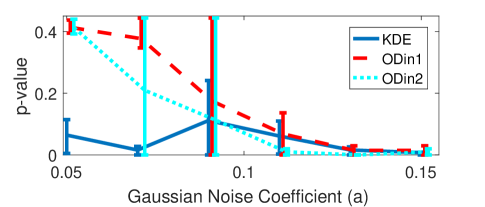
Fig. 2: The average $p$-value with error bars at the 20th and 80th percentiles from 90 trials for the hypothesis test that $G(p;p^{\prime})=1$ after running the CL algorithm for (8). The graphs are offset horizontally for better visualization. Higher noise levels lead to higher error rates in the CL algorithm and thus lower $p$-values.

The final set of experiments focuses on (9). In this case, the CL tree does not include the edge between $\mathbf{X}^{(1)}$ and $\mathbf{X}^{(3)}$ and we report the $p$-values for the hypothesis that $G\left(p;p^{\prime}\right)=1$ when varying either $a$ or $b$. The mean $p$-value with error bars at the 20th and 80th percentiles from 100 trials are given in Figure 3. In the top figure, we fix $b=0.5$ and vary the noise parameter $a$ while in the bottom figure we fix $a=0.05$ and vary $b$. Thus the true structure does not match the CL tree and low $p$-values are desired. For low noise in the top figure (fixed dependency coefficient), the ODin estimators perform better than the KDE estimator and have less variability. In the bottom figure (fixed noise), the ODin1 estimator generally outperforms the other estimators.

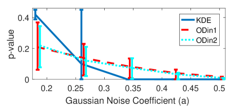
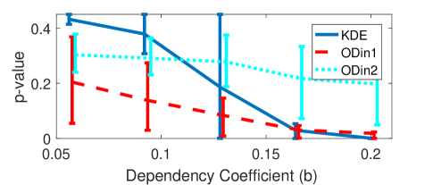
Fig. 3: The mean $p$-value with error bars at the 20th and 80th percentiles from 100 trials for the hypothesis test that $G\left(p;p^{\prime}\right)=1$ for (9) when the CL tree does not give the correct structure. Top: $b=0.5$ and $a$ varies. Bottom: $a=0.05$ and $b$ varies. The graphs are offset horizontally for better visualization. Low $p$-values indicate better performance. The ODin1 estimator generally matches or outperforms the other estimators, especially in the lower noise cases.

In general, the ODin1 estimator outperforms the other estimators in these experiments. Future work includes investigating other scenarios including larger dimensional data and larger sample sizes. Based on the experiments in [27, 25], it is possible that the ODin2 estimator will perform comparably to the ODin1 estimator and that both ODin estimators will outperform the KDE estimator in higher dimensions.

5 Conclusion

We derived the convergence rates for a kernel density plug-in estimator of MI functionals and proposed nonparametric ensemble estimators with a CLT that achieve the parametric rate when the densities are sufficiently smooth. We proposed two approaches for hypothesis testing based on the CLT to learn the structure of the data. The experiments demonstrated the utility of these approaches in structure learning and demonstrated the improvement of ensemble methods over the plug-in method for a low dimensional example.

Appendix A Assumptions

In the proofs, we assume the more general Hölder condition of smoothness on the densities:

Definition 1 (Hölder Class).

Let $\mathcal{X}\subset\mathbb{R}^{d}$ be a compact space. For $r=(r_{1},\dots,r_{d}),$ $r_{i}\in\mathbb{N},$ define $|r|=\sum_{i=1}^{d}r_{i}$ and $D^{r}=\frac{\partial^{|r|}}{\partial x_{1}^{r_{1}}\dots\partial x_{d}^{r_{d}}}$. The Hölder class $\Sigma(s,H)$ of functions on $L_{2}(\mathcal{X})$ consists of the functions $f$ that satisfy

$$\left|D^{r}f(x)-D^{r}f(y)\right|\leq H\left\|x-y\right\|^{s-r},$$

for all $x,\,y\in\mathcal{X}$ and for all $r$ s.t. $|r|\leq\left\lfloor s\right\rfloor$.

Note that if $p\in\Sigma(s,H)$, then $p$ has at least $\left\lfloor s\right\rfloor$ derivatives.

The full assumptions we make on the densities and the functional $g$, which we adapt from [27], are

• $(\mathcal{A}.0)$: Assume that the kernel $K$ is a symmetric product kernel with bounded support in each dimension.

• $(\mathcal{A}.1)$: Assume there exist constants $\epsilon_{0},\epsilon_{\infty}$ such that $0<\epsilon_{0}\leq p(x)\leq\epsilon_{\infty}<\infty,\,\forall x\in\mathcal{S}$ and similarly that the marginal densities and joint pairwise densities are bounded above and below.

• $(\mathcal{A}.2)$: Assume that each of the densities belong to $\Sigma(s,H)$ in the interior of their support sets with $s\geq 2$.

• $(\mathcal{A}.3)$: Assume that $g\left(t_{1}/t_{2}\right)$ has an infinite number of mixed derivatives wrt $t_{1}$ and $t_{2}$.

• $(\mathcal{A}.4$): Assume that $\left|\frac{\partial^{k+l}g(t_{1},t_{2})}{\partial t_{1}^{k}\partial t_{2}^{l}}\right|/(k!l!)$, $k,l=0,1,\ldots$ are strictly upper bounded for $\epsilon_{0}\leq t_{1},t_{2}\leq\epsilon_{\infty}$.

• $(\mathcal{A}.5)$: Assume the following boundary smoothness condition: Let $p_{x}(u):\mathbb{R}^{d}\rightarrow\mathbb{R}$ be a polynomial in $u$ of order $q\leq r=\left\lfloor s\right\rfloor$ whose coefficients are a function of $x$ and are $r-q$ times differentiable. Then assume that

  $$\int_{x\in\mathcal{S}}\left(\int_{u:K(u)>0,\,x+uh\notin\mathcal{S}}K(u)p_{x}(u)du\right)^{t}dx=v_{t}(h),$$

  where $v_{t}(h)$ admits the expansion

  $$v_{t}(h)=\sum_{i=1}^{r-q}e_{i,q,t}h^{i}+o\left(h^{r-q}\right),$$

  for some constants $e_{i,q,t}$.

It has been shown that assumption $\mathcal{A}.5$ is satisfied when $\mathcal{S}$ is rectangular (e.g. $\mathcal{S}=[-1,1]^{d}$) and $K$ is the uniform rectangular kernel [27]. Thus it can be applied to any densities in $\Sigma(s,H)$ on this support.

Appendix B Proof of Bias Results

We prove Theorem 1 in this appendix. The proof shares some similarities with the bias proof of the divergence functional estimators in [27]. The primary differences lie in handling the possible dependencies between random variables. We focus on the more difficult case of $\tilde{\mathbf{G}}_{h}$ as the bias derivation for $\tilde{\mathbf{G}}_{h,ij}$ is similar.

Recall that $\tilde{\mathbf{p}}_{X,h}^{{}^{\prime}}$ is a ratio of two products of KDEs. The numerator is a product of 2-dimensional KDEs while the denominator is a product of marginal (1-dimensional) KDEs, all with the same bandwidth. Let $\gamma\subset\left\{(i,j):i,j\in\left\{1,\dots,d\right\}\right\}$ denote the set of index pairs that denote the components of $\mathbf{X}$ that have joint KDEs that are in the product in the numerator of $\tilde{\mathbf{p}}_{X,h}^{{}^{\prime}}$. Let $\beta$ denote the set of indices that denote the components of $\mathbf{X}$ that have marginal KDEs that are in the product in the denominator of $\tilde{\mathbf{p}}_{X,h}^{{}^{\prime}}$. Note that $|\gamma|=d-1$ and $|\beta|=d-2$. As an example, in the example given in (4), we have $\gamma=\left\{(1,2),(2,3)\right\}$ and $\beta=\{2\}$. The bias of $\tilde{\mathbf{G}}_{h}$ can then be expressed as

$$\mathbb{B}\left[\tilde{\mathbf{G}}_{h}\right] =\mathbb{E}\left[g\left(\frac{\tilde{\mathbf{p}}_{X,h}^{{}^{\prime}}(\mathbf{X})}{\tilde{\mathbf{p}}_{X,h}(\mathbf{X})}\right)-g\left(\frac{p^{\prime}(\mathbf{X})}{p(\mathbf{X})}\right)\right]$$

$$=\mathbb{E}\left[g\left(\frac{\tilde{\mathbf{p}}_{X,h}^{{}^{\prime}}(\mathbf{X})}{\tilde{\mathbf{p}}_{X,h}(\mathbf{X})}\right)-g\left(\frac{\prod_{(i,j)\in\gamma}\mathbb{E}_{\mathbf{X}}\left[\tilde{\mathbf{p}}_{ij,h}\left(\mathbf{X}^{(i)},\mathbf{X}^{(j)}\right)\right]}{\mathbb{E}_{\mathbf{X}}\left[\tilde{\mathbf{p}}_{X,h}(\mathbf{X})\right]\prod_{k\in\beta}\mathbb{E}_{\mathbf{X}}\left[\tilde{\mathbf{p}}_{k,h}\left(\mathbf{X}^{(k)}\right)\right]}\right)\right]$$

$$+\mathbb{E}\left[g\left(\frac{\prod_{(i,j)\in\gamma}\mathbb{E}_{\mathbf{X}}\left[\tilde{\mathbf{p}}_{ij,h}\left(\mathbf{X}^{(i)},\mathbf{X}^{(j)}\right)\right]}{\mathbb{E}_{\mathbf{X}}\left[\tilde{\mathbf{p}}_{X,h}(\mathbf{X})\right]\prod_{k\in\beta}\mathbb{E}_{\mathbf{X}}\left[\tilde{\mathbf{p}}_{k,h}\left(\mathbf{X}^{(k)}\right)\right]}\right)-g\left(\frac{p^{\prime}(\mathbf{X})}{p(\mathbf{X})}\right)\right],$$ (10)

where $\mathbf{X}$ is drawn from $p$ and $\mathbb{E}_{\mathbf{X}}$ denotes the conditional expectation given $\mathbf{X}$. We can view these terms as a variance-like component (the first term) and a bias-like component, where the respective Taylor series expansions depend on variance-like or bias-like terms of the KDEs.

We first consider the bias-like term, i.e. the second term in (10). The Taylor series expansion of $g\left(\frac{\prod_{(i,j)\in\gamma}\mathbb{E}_{\mathbf{X}}\left[\tilde{\mathbf{p}}_{ij,h}\left(\mathbf{X}^{(i)},\mathbf{X}^{(j)}\right)\right]}{\mathbb{E}_{\mathbf{X}}\left[\tilde{\mathbf{p}}_{X,h}(\mathbf{X})\right]\prod_{k\in\beta}\mathbb{E}_{\mathbf{X}}\left[\tilde{\mathbf{p}}_{k,h}\left(\mathbf{X}^{(k)}\right)\right]}\right)$ around $\prod_{(i,j)\in\gamma}p\left(\mathbf{X}^{(i)},\mathbf{X}^{(j)}\right)$ and $p(\mathbf{X})\prod_{k\in\gamma}p(\mathbf{X}^{(k)})$ gives an expansion with terms of the form of

$$\mathbb{B}_{\mathbf{X}}^{m}\left[\prod_{(i,j)\in\gamma}\tilde{\mathbf{p}}_{ij,h}\left(\mathbf{X}^{(i)},\mathbf{X}^{(j)}\right)\right] =\left(\prod_{(i,j)\in\gamma}\mathbb{E}_{\mathbf{X}}\left[\tilde{\mathbf{p}}_{ij,h}\left(\mathbf{X}^{(i)},\mathbf{X}^{(j)}\right)\right]-\prod_{(i,j)\in\gamma}p\left(\mathbf{X}^{(i)},\mathbf{X}^{(j)}\right)\right)^{m},$$

$$\mathbb{B}_{\mathbf{X}}^{m}\left[p(\mathbf{X})\prod_{k\in\gamma}p(\mathbf{X}^{(k)})\right] =\left(\mathbb{E}_{\mathbf{X}}\left[\tilde{\mathbf{p}}_{X,h}(\mathbf{X})\right]\prod_{k\in\beta}\mathbb{E}_{\mathbf{X}}\left[\tilde{\mathbf{p}}_{k,h}\left(\mathbf{X}^{(k)}\right)\right]-p(\mathbf{X})\prod_{k\in\gamma}p(\mathbf{X}^{(k)})\right)^{m}.$$

Since we are not doing boundary correction, we need to consider separately the cases when $\mathbf{X}$ is in the interior of the support $\mathcal{S}$ and when $\mathbf{X}$ is close to the boundary of the support. For precise definitions, a point $X\in\mathcal{S}$ is in the interior of $\mathcal{S}$ if for all $X^{{}^{\prime}}\notin\mathcal{S}$, $K\left(\frac{X-X^{{}^{\prime}}}{h}\right)=0$, and a point $X\in\mathcal{S}$ is near the boundary of the support if it is not in the interior. Since $K$ is a product kernel, $X\in\mathcal{S}$ is in the interior if and only if all of the components of $X$ are in their respective interiors.

Assume that $\mathbf{X}$ is drawn from the interior of $\mathcal{S}$. By a Taylor series expansion of the probability density $p$, we have that

$$\mathbb{E}_{\mathbf{X}}\left[\tilde{\mathbf{p}}_{X,h}(\mathbf{X})\right] =\frac{1}{h^{d}}\int K\left(\frac{\mathbf{X}-x}{h}\right)p\left(x\right)dx$$

$$=\int K(u)p(\mathbf{X}-uh)du$$

$$=p(\mathbf{X})+\sum_{j=1}^{\left\lfloor s/2\right\rfloor}c_{X,j}(\mathbf{X})h^{2j}+O\left(h^{s}\right).$$ (11)

Similar expressions can be obtained for $\mathbb{E}_{\mathbf{X}}\left[\tilde{\mathbf{p}}_{ij,h}\left(\mathbf{X}^{(i)},\mathbf{X}^{(j)}\right)\right]$ and $\mathbb{E}_{\mathbf{X}}\left[\tilde{\mathbf{p}}_{k,h}\left(\mathbf{X}^{(k)}\right)\right]$.

Now assume that $\mathbf{X}$ lies near the boundary of the support $\mathcal{S}$. In this case, we extend the expectation beyond the support of the density:

$$\mathbb{E}_{\mathbf{X}}\left[\tilde{\mathbf{p}}_{X,h}(\mathbf{X})\right]-p(\mathbf{X}) =\frac{1}{h^{d}}\int_{x:x\in\mathcal{S}}K\left(\frac{\mathbf{X}-x}{h}\right)p(x)dx-p(\mathbf{X})$$

$$=\left[\frac{1}{h^{d}}\int_{x:K\left(\frac{\mathbf{X}-x}{h}\right)>0}K\left(\frac{\mathbf{X}-x}{h}\right)p(x)dx-p(\mathbf{X})\right]$$

$$-\left[\frac{1}{h^{d}}\int_{x:x\notin\mathcal{S}}K\left(\frac{\mathbf{X}-x}{h}\right)p(x)dx\right]$$

$$=T_{1,X}(\mathbf{X})-T_{2,X}(\mathbf{X}).$$ (12)

We only evaluate the density $p$ and its derivatives at points within the support when we take its Taylor series expansion. Thus the exact manner in which we define the extension of $p$ does not matter as long as the Taylor series remains the same and as long as the extension is smooth. Thus the expected value of $T_{1,X}(\mathbf{X})$ gives an expression of the form of (11). For the $T_{2,X}(\mathbf{X})$ term, we perform a similar Taylor series expansion and then apply the condition in assumption $\mathcal{A}.5$ to obtain

$$\mathbb{E}\left[T_{2,X}(\mathbf{X})\right]=\sum_{i=1}^{r}e_{i}h^{i}+o\left(h^{r}\right).$$

Similar expressions can be found for $\tilde{\mathbf{p}}_{ij,h}\left(\mathbf{X}^{(i)},\mathbf{X}^{(j)}\right)$ , $\tilde{\mathbf{p}}_{k,h}\left(\mathbf{X}^{(k)}\right)$, and when (12) is raised to a power $t$. Applying this result gives for the second term in (10),

$$\sum_{j=1}^{r}c_{g,p,j}h^{j}+O\left(h^{s}\right),$$ (13)

where the constants $c_{g,p,j}$ depend on the densities, their derivatives, and the functional $g$ and its derivatives.

For the first term in (10), a Taylor series expansion of $g\left(\frac{\tilde{\mathbf{p}}_{X,h}^{{}^{\prime}}(\mathbf{X})}{\tilde{\mathbf{p}}_{X,h}(\mathbf{X})}\right)$ around $\prod_{(i,j)\in\gamma}\mathbb{E}_{\mathbf{X}}\left[\tilde{\mathbf{p}}_{ij,h}\left(\mathbf{X}^{(i)},\mathbf{X}^{(j)}\right)\right]$ and
$\mathbb{E}_{\mathbf{X}}\left[\tilde{\mathbf{p}}_{X,h}(\mathbf{X})\right]\prod_{k\in\beta}\mathbb{E}_{\mathbf{X}}\left[\tilde{\mathbf{p}}_{k,h}\left(\mathbf{X}^{(k)}\right)\right]$ gives an expansion with terms of the form of

$$\tilde{\mathbf{e}}_{1,h}^{q}(\mathbf{X}) = \left(\prod_{(i,j)\in\gamma}\tilde{\mathbf{p}}_{ij,h}\left(\mathbf{X}^{(i)},\mathbf{X}^{(j)}\right)-\prod_{(i,j)\in\gamma}\mathbb{E}_{\mathbf{X}}\left[\tilde{\mathbf{p}}_{ij,h}\left(\mathbf{X}^{(i)},\mathbf{X}^{(j)}\right)\right]\right)^{q},$$

$$\tilde{\mathbf{e}}_{2,h}^{q}(\mathbf{X}) = \left(\tilde{\mathbf{p}}_{X,h}(\mathbf{X})\prod_{k\in\beta}\tilde{\mathbf{p}}_{k,h}\left(\mathbf{X}^{(k)}\right)-\mathbb{E}_{\mathbf{X}}\left[\tilde{\mathbf{p}}_{X,h}(\mathbf{X})\right]\prod_{k\in\beta}\mathbb{E}_{\mathbf{X}}\left[\tilde{\mathbf{p}}_{k,h}\left(\mathbf{X}^{(k)}\right)\right]\right)^{q}.$$

To control these terms, we need expressions for $\mathbb{E}_{\mathbf{X}}\left[\tilde{\mathbf{e}}_{1,h}^{q}(\mathbf{X})\right]$ and $\mathbb{E}_{\mathbf{X}}\left[\tilde{\mathbf{e}}_{2,h}^{q}(\mathbf{X})\right]$. We’ll derive the expression only for $\mathbb{E}_{\mathbf{X}}\left[\tilde{\mathbf{e}}_{1,h}^{q}(\mathbf{X})\right]$ as the expression for $\mathbb{E}_{\mathbf{X}}\left[\tilde{\mathbf{e}}_{2,h}^{q}(\mathbf{X})\right]$ is obtained in a similar manner.

For simplicity of exposition, we assume that $d=3$ and that $\gamma=\left\{(1,2),(2,3)\right\}$. Note that our method extends easily to the general case where notation can be cumbersome. Define

$$\mathbf{V}_{i,j}(\mathbf{X}) =K_{1}\left(\frac{\mathbf{X}^{(1)}_{i}-\mathbf{X}^{(1)}}{h}\right)K_{2}\left(\frac{\mathbf{X}^{(2)}_{i}-\mathbf{X}^{(2)}}{h}\right)K_{2}\left(\frac{\mathbf{X}^{(2)}_{j}-\mathbf{X}^{(2)}}{h}\right)K_{3}\left(\frac{\mathbf{X}^{(3)}_{j}-\mathbf{X}^{(3)}}{h}\right)$$

$$-\mathbb{E}_{\mathbf{X}}\left[K_{1}\left(\frac{\mathbf{X}^{(1)}_{i}-\mathbf{X}^{(1)}}{h}\right)K_{2}\left(\frac{\mathbf{X}^{(2)}_{i}-\mathbf{X}^{(2)}}{h}\right)\right]\mathbb{E}_{\mathbf{X}}\left[K_{2}\left(\frac{\mathbf{X}^{(2)}_{j}-\mathbf{X}^{(2)}}{h}\right)K_{3}\left(\frac{\mathbf{X}^{(3)}_{j}-\mathbf{X}^{(3)}}{h}\right)\right]$$

$$=\mathbf{\eta}_{ij}(\mathbf{X})-\mathbb{E}_{\mathbf{X}}\left[\mathbf{\eta}_{i}(\mathbf{X})\right]\mathbb{E}_{\mathbf{X}}\left[\mathbf{\eta}_{j}^{{}^{\prime}}(\mathbf{X})\right].$$

Therefore,

$$\tilde{\mathbf{e}}_{1,h}(\mathbf{X})=\frac{1}{\left(Nh^{2}\right)^{|\gamma|}}\sum_{i=1}^{N}\sum_{j=1}^{N}\mathbf{V}_{i,j}(\mathbf{X}).$$

By the binomial theorem,

$$\mathbb{E}_{\mathbf{X}}\left[\mathbf{V}_{i,j}^{k}(\mathbf{X})\right]=\sum_{l=0}^{k}\binom{l}{k}\mathbb{E}_{\mathbf{X}}\left[\mathbf{\eta}_{ij}^{l}(\mathbf{X})\right]\left[\mathbb{E}_{\mathbf{X}}\left[\eta_{i}(\mathbf{X})\right]\mathbb{E}_{\mathbf{X}}\left[\eta_{j}^{{}^{\prime}}(\mathbf{X})\right]\right]^{k-l}.$$

It can then be seen using a similar Taylor Series analysis as in the derivation of (11) that for $\mathbf{X}$ in the interior of $\mathcal{S}$ and $i\neq j$, we have that

$$\mathbb{E}_{\mathbf{X}}\left[\mathbf{\eta}_{ij}^{l}(\mathbf{X})\right]=h^{2|\gamma|}\sum_{m=0}^{\left\lfloor s/2\right\rfloor}c_{2,1,m,l}(\mathbf{X})h^{2m}.$$

Combining these results gives for $i\neq j$

$$\mathbb{E}_{\mathbf{X}}\left[\mathbf{V}_{i,j}^{k}(\mathbf{X})\right]=h^{2|\gamma|}\sum_{m=0}^{\left\lfloor s/2\right\rfloor}c_{2,2,m,k}(\mathbf{X})h^{2m}+O\left(h^{4|\gamma|}\right).$$

If $i=j$, we obtain

$$\mathbb{E}_{\mathbf{X}}\left[\mathbf{\eta}_{ii}^{l}(\mathbf{X})\right]=h^{d}\sum_{m=0}^{\left\lfloor s/2\right\rfloor}c_{2,2,m}(\mathbf{X})h^{2m}.$$

This then gives

$$\mathbb{E}_{\mathbf{X}}\left[\mathbf{V}_{i,i}^{k}(\mathbf{X})\right]=h^{d}\sum_{m=0}^{\left\lfloor s/2\right\rfloor}c_{2,m,k}(\mathbf{X})h^{2m}+O\left(h^{4|\gamma|}\right)$$

Here the constants $c_{2,i,m,k}(\mathbf{X})$ depend on the density $p$, its derivatives, and the moments of the kernels.

Let $n(q)$ be the set of integer divisors of $q$ including 1 but excluding $q$. Then due to the independence of the different samples, it can then be shown that

$$\mathbb{E}_{\mathbf{X}}\left[\tilde{\mathbf{e}}_{1,h}^{q}(\mathbf{X})\right]=\sum_{i\in n(q)}\sum_{m=0}^{\left\lfloor s/2\right\rfloor}\left(\frac{c_{3,1,m,q}(\mathbf{X})}{\left(Nh^{2}\right)^{(q-i)}}+\frac{c_{3,2,m,q}(\mathbf{X})}{\left(Nh\right)^{(q-i)}}\right)h^{2m}+o\left(\frac{1}{N}\right).$$ (14)

By a similar procedure, we can show that

$$\mathbb{E}_{\mathbf{X}}\left[\tilde{\mathbf{e}}_{2,h}^{q}(\mathbf{X})\right]=\sum_{i\in n(q)}\sum_{m=0}^{\left\lfloor s/2\right\rfloor}\left(\sum_{j=0}^{|\beta|}\frac{c_{4,1,j,m,q}(\mathbf{X})}{\left(Nh^{d}\left(Nh\right)^{j}\right)^{q-i}}+\frac{c_{4,2,m,q}(\mathbf{X})}{\left(Nh\right)^{q-i}}\right)h^{2m}+o\left(\frac{1}{N}\right).$$ (15)

When $\mathbf{X}$ is near the boundary of the support, we can obtain similar expressions as in (14) and (15) by following a similar procedure as in the derivation of (13). The primary difference is that we will then have powers of $h^{m}$ instead of $h^{2m}$.

For general $g$, we can only guarantee that

$$c\left(\frac{\prod_{(i,j)\in\gamma}\mathbb{E}_{\mathbf{X}}\left[\tilde{\mathbf{p}}_{ij,h}\left(\mathbf{X}^{(i)},\mathbf{X}^{(j)}\right)\right]}{\mathbb{E}_{\mathbf{X}}\left[\tilde{\mathbf{p}}_{X,h}(\mathbf{X})\right]\prod_{k\in\beta}\mathbb{E}_{\mathbf{X}}\left[\tilde{\mathbf{p}}_{k,h}\left(\mathbf{X}^{(k)}\right)\right]}\right)=c\left(\frac{p^{\prime}(\mathbf{X})}{p(\mathbf{X})}\right)+o(1),$$

where $c(t_{1},t_{2})$ is a functional of the derivatives of $g$. Applying this gives the final result in this case. However, we can obtain higher order terms by making stronger assumptions on the functional $g$ and its derivatives. Specifically, if $c(t_{1},t_{2})$ includes functionals of the form of $t_{1}^{\alpha}t_{2}^{\beta}$ with $\alpha,\beta<0$, then we can apply the generalized binomial theorem to use the higher order expressions in (14) and (15). This completes the proof.

Appendix C Proof of Variance Results

To bound the variance of the plug-in estmiator, we use the Efron-Stein inequality [28]:

Lemma 4.

(Efron-Stein Inequality) Let $\mathbf{X}_{1},\dots,\mathbf{X}_{n},\mathbf{X}_{1}^{{}^{\prime}},\dots,\mathbf{X}_{n}^{{}^{\prime}}$ be independent random variables on the space $\mathcal{S}$. Then if $f:\mathcal{S}\times\dots\times\mathcal{S}\rightarrow\mathbb{R}$, we have that

$$\mathbb{V}\left[f(\mathbf{X}_{1},\dots,\mathbf{X}_{n})\right]\leq\frac{1}{2}\sum_{i=1}^{n}\mathbb{E}\left[\left(f(\mathbf{X}_{1},\dots,\mathbf{X}_{n})-f(\mathbf{X}_{1},\dots,\mathbf{X}_{i}^{{}^{\prime}},\dots,\mathbf{X}_{n})\right)^{2}\right].$$

The Efron-Stein inequality bounds the variance by the sum of the expected squared difference between the plug-in estimator with the original samples and the plug-in estimator where one of the samples is replaced with another iid sample.

In our case, consider the sample sets $\left\{\mathbf{X}_{1},\dots,\mathbf{X}_{n}\right\}$ and $\left\{\mathbf{X}_{1}^{{}^{\prime}},\mathbf{X}_{2}\dots,\mathbf{X}_{n}\right\}$ and denote the respective plug-in estimators as $\tilde{\mathbf{G}}_{h}$ and $\tilde{\mathbf{G}}_{h}^{{}^{\prime}}$. Using the triangle inequality, we have

$$\left|\tilde{\mathbf{G}}_{h}-\tilde{\mathbf{G}}_{h}^{{}^{\prime}}\right| \leq\frac{1}{N}\left|g\left(\frac{\tilde{\mathbf{p}}_{X,h}^{{}^{\prime}}(\mathbf{X}_{1})}{\tilde{\mathbf{p}}_{X,h}(\mathbf{X}_{1})}\right)-g\left(\frac{\tilde{\mathbf{p}}_{X,h}^{{}^{\prime}}(\mathbf{X}_{1}^{{}^{\prime}})}{\tilde{\mathbf{p}}_{X,h}(\mathbf{X}_{1}^{{}^{\prime}})}\right)\right|+\frac{1}{N}\sum_{j=2}^{N}\left|g\left(\frac{\tilde{\mathbf{p}}_{X,h}^{{}^{\prime}}(\mathbf{X}_{j})}{\tilde{\mathbf{p}}_{X,h}(\mathbf{X}_{j})}\right)-g\left(\frac{\left(\tilde{\mathbf{p}}_{X,h}^{{}^{\prime}}(\mathbf{X}_{j})\right)^{{}^{\prime}}}{\left(\tilde{\mathbf{p}}_{X,h}(\mathbf{X}_{j})\right)^{{}^{\prime}}}\right)\right|,$$ (16)

where $\left(\tilde{\mathbf{p}}_{X,h}^{{}^{\prime}}(\mathbf{X}_{j})\right)^{{}^{\prime}}$ and $\left(\tilde{\mathbf{p}}_{X,h}(\mathbf{X}_{j})\right)^{{}^{\prime}}$ are the respective KDEs with $\mathbf{X}_{1}$ replaced with $\mathbf{X}_{1}^{{}^{\prime}}$. Then since $g$ is Lipschitz continuous with constant $C_{g}$, we can write

$$\left|g\left(\frac{\tilde{\mathbf{p}}_{X,h}^{{}^{\prime}}(\mathbf{X}_{1})}{\tilde{\mathbf{p}}_{X,h}(\mathbf{X}_{1})}\right)-g\left(\frac{\tilde{\mathbf{p}}_{X,h}^{{}^{\prime}}(\mathbf{X}_{1}^{{}^{\prime}})}{\tilde{\mathbf{p}}_{X,h}(\mathbf{X}_{1}^{{}^{\prime}})}\right)\right| \leq C_{g}\left|\prod_{(i,j)\in\gamma}\tilde{\mathbf{p}}_{ij,h}\left(\mathbf{X}^{(i)}_{1},\mathbf{X}^{(j)}_{1}\right)-\prod_{(i,j)\in\gamma}\tilde{\mathbf{p}}_{ij,h}\left(\mathbf{X}^{{}^{\prime}(i)}_{1},\mathbf{X}^{{}^{\prime}(j)}_{1}\right)\right|$$

$$+C_{g}\left|\tilde{\mathbf{p}}_{X,h}(\mathbf{X}_{1})\prod_{k\in\beta}\tilde{\mathbf{p}}_{k,h}\left(\mathbf{X}^{(k)}_{1}\right)-\tilde{\mathbf{p}}_{X,h}(\mathbf{X}_{1}^{{}^{\prime}})\prod_{k\in\beta}\tilde{\mathbf{p}}_{k,h}\left(\mathbf{X}^{{}^{\prime}(k)}_{1}\right)\right|.$$

To bound the expected squared value of these terms, we split the product of KDEs into separate cases. For example, if we consider the case where the KDEs are all evaluated at the same point which occurs $M$ times, we obtain

$$\frac{M}{\left(Mh^{2}\right)^{2|\gamma|}}\sum_{m=2}^{N}\mathbb{E}\left[\left(\prod_{(i,j)\in\gamma}K_{i}\left(\frac{\mathbf{X}^{(i)}_{1}-\mathbf{X}^{(i)}_{m}}{h}\right)K_{j}\left(\frac{\mathbf{X}^{(j)}_{1}-\mathbf{X}^{(j)}_{m}}{h}\right)-\prod_{(i,j)\in\gamma}K_{i}\left(\frac{\mathbf{X}^{{}^{\prime}(i)}_{1}-\mathbf{X}^{(i)}_{m}}{h}\right)K_{j}\left(\frac{\mathbf{X}^{{}^{\prime}(j)}_{1}-\mathbf{X}^{(j)}_{m}}{h}\right)\right)^{2}\right]$$

$$\leq\frac{1}{M^{2}}\prod_{(i,j)\in\gamma}||K_{i}K_{j}||_{\infty}^{2}.$$

By considering the other $|\gamma|-1$ cases where the KDEs are evaluated at different points (e.g. 2 KDEs evaluated at the same point while all others are evaluated at different points, etc.), applying Jensen’s inequality gives

$$\mathbb{E}\left[\left|\prod_{(i,j)\in\gamma}\tilde{\mathbf{p}}_{ij,h}\left(\mathbf{X}^{(i)}_{1},\mathbf{X}^{(j)}_{1}\right)-\prod_{(i,j)\in\gamma}\tilde{\mathbf{p}}_{ij,h}\left(\mathbf{X}^{{}^{\prime}(i)}_{1},\mathbf{X}^{{}^{\prime}(j)}_{1}\right)\right|^{2}\right]\leq C_{1}\prod_{(i,j)\in\gamma}||K_{i}K_{j}||_{\infty}^{2},$$

where $C_{1}<\infty$ is some constant that is $O(1)$. Similarly, we obtain

$$\mathbb{E}\left[\left|\tilde{\mathbf{p}}_{X,h}(\mathbf{X}_{1})\prod_{k\in\beta}\tilde{\mathbf{p}}_{k,h}\left(\mathbf{X}^{(k)}_{1}\right)-\tilde{\mathbf{p}}_{X,h}(\mathbf{X}_{1}^{{}^{\prime}})\prod_{k\in\beta}\tilde{\mathbf{p}}_{k,h}\left(\mathbf{X}^{{}^{\prime}(k)}_{1}\right)\right|^{2}\right]\leq C_{2}||K||_{\infty}^{2}\prod_{k\in\beta}||K_{k}||_{\infty}^{2}.$$

Combining these results gives

$$\mathbb{E}\left[\left|g\left(\frac{\tilde{\mathbf{p}}_{X,h}^{{}^{\prime}}(\mathbf{X}_{1})}{\tilde{\mathbf{p}}_{X,h}(\mathbf{X}_{1})}\right)-g\left(\frac{\tilde{\mathbf{p}}_{X,h}^{{}^{\prime}}(\mathbf{X}_{1}^{{}^{\prime}})}{\tilde{\mathbf{p}}_{X,h}(\mathbf{X}_{1}^{{}^{\prime}})}\right)\right|^{2}\right]\leq C_{3},$$ (17)

where $C_{3}=O(1)$.

As before, the Lipschitz condition can be applied to the second term in (16) to obtain

$$\left|g\left(\frac{\tilde{\mathbf{p}}_{X,h}^{{}^{\prime}}(\mathbf{X}_{m})}{\tilde{\mathbf{p}}_{X,h}(\mathbf{X}_{m})}\right)-g\left(\frac{\left(\tilde{\mathbf{p}}_{X,h}^{{}^{\prime}}(\mathbf{X}_{m})\right)^{{}^{\prime}}}{\left(\tilde{\mathbf{p}}_{X,h}(\mathbf{X}_{m})\right)^{{}^{\prime}}}\right)\right| \leq C_{g}\left|\prod_{(i,j)\in\gamma}\tilde{\mathbf{p}}_{ij,h}\left(\mathbf{X}^{(i)}_{m},\mathbf{X}^{(j)}_{m}\right)-\prod_{(i,j)\in\gamma}\tilde{\mathbf{p}}_{ij,h}^{{}^{\prime}}\left(\mathbf{X}^{(i)}_{m},\mathbf{X}^{(j)}_{m}\right)\right|$$

$$+C_{g}\left|\tilde{\mathbf{p}}_{X,h}(\mathbf{X}_{m})\prod_{k\in\beta}\tilde{\mathbf{p}}_{k,h}\left(\mathbf{X}^{(k)}_{m}\right)-\tilde{\mathbf{p}}_{X,h}^{{}^{\prime}}(\mathbf{X}_{m})\prod_{k\in\beta}\tilde{\mathbf{p}}_{k,h}^{{}^{\prime}}\left(\mathbf{X}^{(k)}_{m}\right)\right|.$$

For the first term, we again consider the $|\gamma|$ cases where the KDEs are evaluated at different points. As a concrete example, consider the example given in (4). Then we can write by the triangle inequality

$$\left|\prod_{(i,j)\in\gamma}\tilde{\mathbf{p}}_{ij,h}\left(\mathbf{X}^{(i)}_{m},\mathbf{X}^{(j)}_{m}\right)-\prod_{(i,j)\in\gamma}\tilde{\mathbf{p}}_{ij,h}^{{}^{\prime}}\left(\mathbf{X}^{(i)}_{m},\mathbf{X}^{(j)}_{m}\right)\right|$$

$$\leq\frac{1}{M^{2}h^{4}}\left|K_{1}\left(\frac{\mathbf{X}^{(1)}_{m}-\mathbf{X}^{(1)}_{1}}{h}\right)K_{2}^{2}\left(\frac{\mathbf{X}^{(2)}_{m}-\mathbf{X}^{(2)}_{1}}{h}\right)K_{3}\left(\frac{\mathbf{X}^{(3)}_{m}-\mathbf{X}^{(3)}_{1}}{h}\right)-K_{1}\left(\frac{\mathbf{X}^{(1)}_{m}-\mathbf{X}^{{}^{\prime}(1)}_{1}}{h}\right)K_{2}^{2}\left(\frac{\mathbf{X}^{(2)}_{m}-\mathbf{X}^{{}^{\prime}(2)}_{1}}{h}\right)K_{3}\left(\frac{\mathbf{X}^{(3)}_{m}-\mathbf{X}^{{}^{\prime}(3)}_{1}}{h}\right)\right|$$

$$+\frac{1}{M^{2}h^{4}}\left(\sum_{\begin{subarray}{c}n=2\\ n\neq m\end{subarray}}^{N}K_{1}\left(\frac{\mathbf{X}^{(1)}_{m}-\mathbf{X}^{(1)}_{n}}{h}\right)K_{2}\left(\frac{\mathbf{X}^{(2)}_{m}-\mathbf{X}^{(2)}_{n}}{h}\right)\left|K_{2}\left(\frac{\mathbf{X}^{(2)}_{m}-\mathbf{X}^{(2)}_{1}}{h}\right)K_{3}\left(\frac{\mathbf{X}^{(3)}_{m}-\mathbf{X}^{(3)}_{1}}{h}\right)\right.\right.$$

$$\left.-K_{2}\left(\frac{\mathbf{X}^{(2)}_{m}-\mathbf{X}^{{}^{\prime}(2)}_{1}}{h}\right)K_{3}\left(\frac{\mathbf{X}^{(3)}_{m}-\mathbf{X}^{{}^{\prime}(3)}_{1}}{h}\right)\right|+\left|K_{1}\left(\frac{\mathbf{X}^{(1)}_{m}-\mathbf{X}^{(1)}_{1}}{h}\right)K_{2}\left(\frac{\mathbf{X}^{(2)}_{m}-\mathbf{X}^{(2)}_{1}}{h}\right)-K_{1}\left(\frac{\mathbf{X}^{(1)}_{m}-\mathbf{X}^{{}^{\prime}(1)}_{1}}{h}\right)K_{2}\left(\frac{\mathbf{X}^{(2)}_{m}-\mathbf{X}^{{}^{\prime}(2)}_{1}}{h}\right)\right|$$

$$\left.\times\sum_{\begin{subarray}{c}n=2\\ n\neq m\end{subarray}}^{N}K_{2}\left(\frac{\mathbf{X}^{(2)}_{m}-\mathbf{X}^{(2)}_{n}}{h}\right)K_{3}\left(\frac{\mathbf{X}^{(3)}_{m}-\mathbf{X}^{(3)}_{n}}{h}\right)\right).$$

$$\implies\mathbb{E}\left[\left|\prod_{(i,j)\in\gamma}\tilde{\mathbf{p}}_{ij,h}\left(\mathbf{X}^{(i)}_{m},\mathbf{X}^{(j)}_{m}\right)-\prod_{(i,j)\in\gamma}\tilde{\mathbf{p}}_{ij,h}^{{}^{\prime}}\left(\mathbf{X}^{(i)}_{m},\mathbf{X}^{(j)}_{m}\right)\right|^{2}\right]\leq\frac{4+6(M-2)^{2}}{M^{4}}||K_{1}K_{2}^{2}K_{3}||_{\infty}^{2}.$$ (18)

For more general $\gamma$, it can be shown that the LHS of (18) is $O\left(\frac{1}{M^{2}}\right)$. Similarly, we can check that

$$\mathbb{E}\left[\left|\tilde{\mathbf{p}}_{X,h}(\mathbf{X}_{m})\prod_{k\in\beta}\tilde{\mathbf{p}}_{k,h}\left(\mathbf{X}^{(k)}_{m}\right)-\tilde{\mathbf{p}}_{X,h}^{{}^{\prime}}(\mathbf{X}_{m})\prod_{k\in\beta}\tilde{\mathbf{p}}_{k,h}^{{}^{\prime}}\left(\mathbf{X}^{(k)}_{m}\right)\right|^{2}\right]=O\left(\frac{1}{M^{2}}\right).$$

Applying the Cauchy-Schwarz inequality with these results then gives

$$\mathbb{E}\left[\left(\sum_{j=2}^{N}\left|g\left(\frac{\tilde{\mathbf{p}}_{X,h}^{{}^{\prime}}(\mathbf{X}_{j})}{\tilde{\mathbf{p}}_{X,h}(\mathbf{X}_{j})}\right)-g\left(\frac{\left(\tilde{\mathbf{p}}_{X,h}^{{}^{\prime}}(\mathbf{X}_{j})\right)^{{}^{\prime}}}{\left(\tilde{\mathbf{p}}_{X,h}(\mathbf{X}_{j})\right)^{{}^{\prime}}}\right)\right|\right)^{2}\right]=O(1).$$ (19)

Combining (17) and (19) with (16) gives

$$\mathbb{E}\left[\left|\tilde{\mathbf{G}}_{h}-\tilde{\mathbf{G}}_{h}^{{}^{\prime}}\right|^{2}\right]=O\left(\frac{1}{N^{2}}\right).$$

Applying the Efron-Stein inequality then gives

$$\mathbb{V}\left[\tilde{\mathbf{G}}_{h}\right]=O\left(\frac{1}{N}\right).$$

References

[1]
T. M. Cover and J. A. Thomas,
Elements of information theory,
John Wiley & Sons, 2012.
[2]
Paul Viola and William M Wells III,
“Alignment by maximization of mutual information,”
International journal of computer vision, vol. 24, no. 2, pp.
137–154, 1997.
[3]
Dávid Pál, Barnabás Póczos, and Csaba Szepesvári,
“Estimation of rényi entropy and mutual information based on
generalized nearest-neighbor graphs,”
in Advances in Neural Information Processing Systems, 2010, pp.
1849–1857.
[4]
Pierre Comon,
“Independent component analysis, a new concept?,”
Signal processing, vol. 36, no. 3, pp. 287–314, 1994.
[5]
C Chow and C Liu,
“Approximating discrete probability distributions with dependence
trees,”
IEEE transactions on Information Theory, vol. 14, no. 3, pp.
462–467, 1968.
[7]
Karthik Mohan, Mike Chung, Seungyeop Han, Daniela Witten, Su-In Lee, and Maryam
Fazel,
“Structured learning of gaussian graphical models,”
in Advances in neural information processing systems, 2012, pp.
620–628.
[8]
Ming Yuan and Yi Lin,
“Model selection and estimation in the gaussian graphical model,”
Biometrika, vol. 94, no. 1, pp. 19–35, 2007.
[9]
R. Kindermann and J.L. Snell,
Markov Random Fields and Their Applications,
American Mathematical Society, 1980.
[10]
David Edwards,
Introduction to graphical modelling,
Springer Science & Business Media, 2012.
[11]
Judea Pearl,
Probabilistic reasoning in intelligent systems: networks of
plausible inference,
Morgan Kaufmann, 2014.
[12]
Animashree Anandkumar and Ragupathyraj Valluvan,
“Learning loopy graphical models with latent variables: Efficient
methods and guarantees,”
The Annals of Statistics, vol. 41, no. 2, pp. 401–435, 2013.
[13]
Myung Jin Choi, Vincent YF Tan, Animashree Anandkumar, and Alan S Willsky,
“Learning latent tree graphical models,”
Journal of Machine Learning Research, vol. 12, no. May, pp.
1771–1812, 2011.
[14]
Elchanan Mossel,
“Distorted metrics on trees and phylogenetic forests,”
IEEE/ACM Transactions on Computational Biology and
Bioinformatics (TCBB), vol. 4, no. 1, pp. 108–116, 2007.
[15]
Alexander Kraskov, Harald Stögbauer, and Peter Grassberger,
“Estimating mutual information,”
Physical review E, vol. 69, no. 6, pp. 066138, 2004.
[16]
LF Kozachenko and Nikolai N Leonenko,
“Sample estimate of the entropy of a random vector,”
Problemy Peredachi Informatsii, vol. 23, no. 2, pp. 9–16,
1987.
[17]
Shiraj Khan, Sharba Bandyopadhyay, Auroop R Ganguly, Sunil Saigal, David J
Erickson III, Vladimir Protopopescu, and George Ostrouchov,
“Relative performance of mutual information estimation methods for
quantifying the dependence among short and noisy data,”
Physical Review E, vol. 76, no. 2, pp. 026209, 2007.
[18]
Weihao Gao, Sewoong Oh, and Pramod Viswanath,
“Demystifying fixed k-nearest neighbor information estimators,”
arXiv preprint arXiv:1604.03006, 2016.
[19]
A. Krishnamurthy, K. Kandasamy, B. Poczos, and L. Wasserman,
“Nonparametric estimation of renyi divergence and friends,”
in Proceedings of The 31st International Conference on Machine
Learning, 2014, pp. 919–927.
[20]
S. Singh and B. Póczos,
“Exponential concentration of a density functional estimator,”
in Advances in Neural Information Processing Systems, 2014, pp.
3032–3040.
[21]
Kirthevasan Kandasamy, Akshay Krishnamurthy, Barnabas Poczos, Larry Wasserman,
and James Robins,
“Nonparametric von mises estimators for entropies, divergences and
mutual informations,”
in Advances in Neural Information Processing Systems, 2015, pp.
397–405.
[22]
K. Sricharan, D. Wei, and A. O. Hero,
“Ensemble estimators for multivariate entropy estimation,”
Information Theory, IEEE Transactions on, vol. 59, no. 7, pp.
4374–4388, 2013.
[23]
K. R. Moon and A. O. Hero III,
“Ensemble estimation of multivariate f-divergence,”
in Information Theory (ISIT), 2014 IEEE International Symposium
on. IEEE, 2014, pp. 356–360.
[24]
K. R. Moon and A. O. Hero III,
“Multivariate f-divergence estimation with confidence,”
in Advances in Neural Information Processing Systems, 2014, pp.
2420–2428.
[25]
Kevin R Moon, Kumar Sricharan, Kristjan Greenewald, and Alfred O Hero III,
“Improving convergence of divergence functional ensemble
estimators,”
in 2016 IEEE International Symposium on Information Theory
(ISIT), 2016.
[26]
Dongxiao Zhu, Alfred O Hero, Zhaohui S Qin, and Anand Swaroop,
“High throughput screening of co-expressed gene pairs with
controlled false discovery rate (fdr) and minimum acceptable strength
(mas),”
Journal of Computational Biology, vol. 12, no. 7, pp.
1029–1045, 2005.
[27]
Kevin R Moon, Kumar Sricharan, Kristjan Greenewald, and Alfred O Hero III,
“Nonparametric ensemble estimation of distributional functionals,”
arXiv preprint arXiv:1601.06884v2, 2016.
[28]
Bradley Efron and Charles Stein,
“The jackknife estimate of variance,”
The Annals of Statistics, pp. 586–596, 1981.