Entanglement verification with detection-efficiency mismatch

Abstract

The security analysis of quantum key distribution is difficult to perform when there is efficiency mismatch between various threshold detectors involved in an experimental setup. Even the verification that the device actually performs in the quantum domain, referred to as the task of entanglement verification, is hard to perform. In this article we provide such an entanglement-verification method for characterized detection-efficiency mismatch. Our method does not rely on a cut-off of photon numbers in the optical signal. It can be applied independently of the degrees of freedom involved, thus covering, for example, efficiency mismatch in polarization and time-bin modes, but also in spatial modes. The evaluation of typical experimental scenarios suggests that an increase of detection-efficiency mismatch will drive the performance of a given setup out of the quantum domain.

I Introduction

The ability to verify effective entanglement in observed data is a necessary condition for Alice and Bob to perform secure quantum key distribution (QKD) [1], demonstrate quantum teleportation [2] and realize quantum repeaters [3]. Many methods have been exploited for verifying entanglement. For example, one can apply the positive partial-transpose (PPT) criterion [4, 5], construct symmetric extensions of a quantum state [6], or build expectation-values matrices (EVMs) from experimental observations and apply corresponding entanglement criteria [7, 8, 9, 10, 11]. Also, one can verify entanglement by directly measuring special observables, e.g., Bell inequalities [12] or entanglement witnesses [13, 14]. (See the review paper [15] for a list and discussions of various methods.) For the typical QKD scenarios where Alice sends optical signals to Bob, we can model the underlying quantum state as Alice holding a discrete finite-dimensional system while Bob receiving an infinite-dimensional optical mode. In this case, EVM-based verification methods are particularly useful. They have been well developed [8, 10, 16, 17, 18, 11] and applied to real experiments [19, 20].

Almost all previously known methods for verifying entanglement assume that various threshold detectors involved in an experimental setup are ideal with perfect efficiency . This assumption can be justified when there is no efficiency mismatch between these threshold detectors. In this case, one cannot distinguish no-detection events due to detection inefficiency from those due to transmission loss. For simplicity of analysis, one can lump these two kinds of loss together as a new increased transmission loss followed by ideal threshold detectors with perfect efficiency (see Sect. III.3 for detailed discussions about this treatment). Then, one can verify entanglement and further prove the security of the corresponding QKD protocols.

However, in practice it is hard to build two detectors that have exactly the same efficiency (for example, due to different samples of the fabrication process). In the presence of efficiency mismatch, one cannot treat detection inefficiency in the same way as transmission loss, and so previously known methods cannot be applied for entanglement verification.

A detection-efficiency mismatch can also be induced by an adversary using the fact that a detector can respond to a photon differently depending on degrees of freedom (for example, spatial mode, frequency, or arriving time) rather than those employed to encode information. If an adversary can control these degrees of freedom such that the induced efficiency mismatch is large enough, powerful attacks on QKD systems exist, as demonstrated in Refs. [21] and [22]. In typical experiments the efficiency mismatch may not seem significant, but it still means that the device cannot be covered by an existing security proof.

In this paper we develop a general method to verify entanglement in the presence of detection-efficiency mismatch. The method works as long as the efficiency mismatch is characterized, even if the mismatch depends on degrees of freedom of a photon that are not employed to encode information. We carefully study an implementation of the BB84-QKD prepare-and-measure protocol [23] with polarization encoding, where we take account of the fact that Bob receives signals in the infinite-dimensional mode space with no limit on the number of photons contained in that space. Our method is expected to work for other QKD protocols. The full security proof of QKD protocols with efficiency mismatch is still an open problem and is not addressed in the current paper either, though some essential tools developed here will carry over to such a security proof. Note that Ref. [24] studied the security proof of the BB84-QKD protocol with efficiency mismatch, under the additional assumption that Bob’s system is a photonic qubit. However, this assumption is hard to justify in actual implementations of QKD where threshold detectors are being used.

The remainder of the paper is laid out as follows: In Sect. II, we describe an experimental setup for implementing the BB84-QKD protocol and the efficiency-mismatch models considered. In Sect. III, we outline how our method works and explain details on how to apply the method to the particular experimental setup considered. In Sect. IV, we simulate experimental results according to a toy channel connecting Alice and Bob just for illustration purposes. For this toy channel, we present the bound on the efficiency mismatch in order for Alice and Bob to verify entanglement based only on their observations. Finally we conclude the paper in Sect. V.

II Experimental configuration

For simplicity, in this paper we consider an experimental implementation of the BB84-QKD prepare-and-measure protocol [23] with polarization encoding. In each run of the protocol, Alice prepares an optical signal where all the photons have the same polarization, randomly selected from the horizontal ($H$), vertical ($V$), diagonal ($D$), or anti-diagonal ($A$) polarizations. Then, Alice sends the optical signal to Bob, and Bob randomly selects to measure it either in the horizontal/vertical ($H/V$) basis or the diagonal/anti-diagonal ($D/A$) basis. After many runs of the protocol, if the final measurement results satisfy some conditions (for example, the quantum bit error rate is low enough), Alice and Bob can distill secret keys via some classical post-processing procedure. For the present study of entanglement verification, we only need to consider the quantum phase of the protocol, i.e., the above prepare-and-measure step.

Obviously, in the above implementation there is no entangled state physically shared between Alice and Bob. However, there is another equivalent description, i.e., the source-replacement description [1, 25], of the prepare-and-measure step in a general QKD protocol: In this thought setup, first Alice prepares an entangled state

$$\Ket{\Phi}_{AA^{\prime}}=\sum_{s=1}^{S}\sqrt{p_{s}}\Ket{s}_{A}\Ket{\phi_{s}}_{A^{\prime}},$$ (1)

where $\{\Ket{s}_{A}\}$ is a set of orthogonal states and $p_{s}$ is the probability of preparing the signal state $\Ket{\phi_{s}}$, $s=1,2,...,S$. Second, Alice measures the system $A$ with the projective positive-operator valued measure (POVM) $\{\Ket{s}\Bra{s},s=1,2,...,S\}$, and distributes the corresponding signal state $\Ket{\phi_{s}}$ to Bob. After the action of the channel (or Eve) on system $A^{\prime}$, Bob receives a system $B$ on which Bob performs a measurement. There is no way for Eve or any other party outside of Alice’s lab to tell which description, either the prepare-and-measure or source-replacement description, is implemented at Alice’s side. In the source-replacement description entanglement between Alice’s system $A$ and Bob’s system $B$ (before their respective measurement) is required; otherwise, intercept-resend attacks on the QKD system exist. In this sense, we say that effective entanglement is a necessary condition for secure QKD [1].

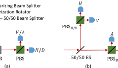
Figure 1: Schematic of the measurement device: (a) is the active-detection scheme where a polarization rotator is used to select a measurement basis, and (b) is the passive-detection scheme where a 50/50 beam splitter is used to select a measurement basis. Under each basis, a polarizing beam splitter and two threshold detectors (which cannot distinguish the number of incoming photons) are used to measure the polarization state of an incoming optical signal. Each detector is labelled by the corresponding measurement outcome.

To measure the polarization state of the incoming optical signal, Bob can employ either the active- or passive-detection scheme, as described in Fig. 1. The detectors involved in each detection scheme are threshold detectors which cannot distinguish the number of incoming photons. So, each detector has only two outcomes, click or no click. However, we do not restrict the number of photons arriving at each detector, due to the following two considerations: First, in practice information is usually encoded in coherent states which actually do have multi-photon components; second, the optical signal prepared by Alice can be intercepted by Eve and replaced by another stronger signal during the transmission from Alice to Bob.

In practice, the efficiencies of each detector are not exactly the same. For the active-detection scheme as shown in Fig. 1(a), the detection efficiency is denoted by $\eta_{H/D}$ if the measurement outcome is $H$ or $D$, and the efficiency is denoted by $\eta_{V/A}$ if the outcome is $V$ or $A$. Similarly, for the passive-detection scheme as shown in Fig. 1(b), there are four detectors corresponding to the four measurement outcomes $H$, $V$, $D$ and $A$. Denote their respective efficiencies by $\eta_{H}$, $\eta_{V}$, $\eta_{D}$ and $\eta_{A}$. We will study entanglement verification in the presence of efficiency mismatch between these detectors. We call this the spatial-mode-independent mismatch model, in contrast to the following mismatch model where the mismatch depends additionally on the spatial modes.

The detection efficiency might not only be different between different detectors of the same build, but there might be also different coupling efficiencies of the detectors to the observed light. This has been demonstrated in recent works [26] and [27], where it has been shown that the coupling efficiency of each detector can be tuned to some degree independently by manipulating the spatial modes of the incoming optical signals. As this kind of spatial-mode-dependent efficiency mismatch is quite relevant especially to implementations of free-space QKD, we would like to study the effect of this mismatch model on entanglement verification. In principle, the number of spatial modes of incoming optical signals can be arbitrary, even infinite. Intuitively, when the number of spatial modes is equal to or larger than the number of detectors in the measurement device, it might become possible for Eve to completely control Bob through the efficiency mismatch. For example, if each detector responds to an optical signal only in a particular spatial mode and different detectors respond to different spatial modes, then Eve can completely effectively switch on and off each detector by sending optical signals in these particular spatial modes. To illustrate the effect of spatial-mode-dependent efficiency mismatch on entanglement verification, we consider the case where the number of spatial modes is equal to the number of detectors. For illustration purposes, we also constrain the mismatch model so that mismatched efficiencies have a permutation symmetry over spatial modes. In particular, the mismatch models considered in the active- and passive-detection schemes are shown as in Tables 1 and 2, respectively. According to the discussion in Sect. III.3, we can renormalize detection efficiencies and treat the common loss in detectors as a part of transmission loss. Hence, we set the maximum detection efficiency in Tables 1 or 2 to be $1$. We would like to stress that we consider these mismatch models just for simplicity and ease of graphical illustrations: The method detailed in the next section works for general mismatch models.

Table 1: Spatial-mode-dependent mismatch model in the active-detection scheme, where $0\leq\eta\leq 1$. Different columns are for different detectors labelled and shown in Fig. 1(a). Different rows are mismatched efficiencies for different spatial modes.

	Det. ‘$H/D$’	Det. ‘$V/A$’
Mode 1	1	$\eta$
Mode 2	$\eta$	1

Table 2: Spatial-mode-dependent mismatch model in the passive-detection scheme, where $0\leq\eta\leq 1$. Different columns are for different detectors labelled and shown in Fig. 1(b). Different rows are mismatched efficiencies for different spatial modes.

	Det. ‘$H$’	Det. ‘$V$’	Det. ‘$D$’	Det. ‘$A$’
Mode 1	1	$\eta$	$\eta$	$\eta$
Mode 2	$\eta$	1	$\eta$	$\eta$
Mode 3	$\eta$	$\eta$	1	$\eta$
Mode 4	$\eta$	$\eta$	$\eta$	1

III Our method

The main idea behind our method is to construct an expectation-values matrix (EVM) [8, 10, 16, 17, 18, 11] using a finite number of actual measurement operators which contain efficiency-mismatch information. Let us discuss the construction and general properties of an EVM before moving on to our particular case.

Suppose that the joint system of Alice and Bob is described by a state $\rho_{AB}$, and that there are two sets of operators $\{\hat{A}_{i}\}$ and $\{\hat{B}_{j}\}$ acting on Alice’s and Bob’s subsystems, respectively. Then, the entries of an EVM $\chi(\rho_{AB})$ are defined  as

$$[\chi(\rho_{AB})]_{ij,kl}=\text{Tr}(\rho_{AB}\hat{A}_{i}^{\dagger}\hat{A}_{k}\otimes\hat{B}_{j}^{\dagger}\hat{B}_{l}).$$ (2)

By the definition, several properties are satisfied by an EVM: First, an EVM is Hermitian and positive-semidefinite. Second, if both the sets of operators $\{\hat{A}_{i}\}$ and $\{\hat{B}_{j}\}$ are finite, the dimension of the EVM $\chi(\rho_{AB})$ is finite even though the state $\rho_{AB}$ is infinite-dimensional. Third, entries of an EVM can be expectation values of observables, if the corresponding measurement operators are included in the set $\{\hat{A}_{i}^{\dagger}\hat{A}_{k}\otimes\hat{B}_{j}^{\dagger}\hat{B}_{l}\}$. Hence, an EVM will be designed as an object into which we can enter all experimental observations (i.e., the probabilities of Alice’s and Bob’s joint measurement outcomes), but there may be undetermined entries. Still, we can study various properties, such as entanglement, of the underlying state. Fourth, the linear relationships between various operators $\hat{A}_{i}^{\dagger}\hat{A}_{k}\otimes\hat{B}_{j}^{\dagger}\hat{B}_{l}$ restrict the entries $\chi_{ij,kl}$. (Here and later, we use $\chi$ and $\chi_{ij,kl}$ as short notations of $\chi(\rho_{AB})$ and $[\chi(\rho_{AB})]_{ij,kl}$ if there is no confusion in the context.) For example, if the operators satisfy

$$\sum_{ijkl}C_{ij,kl}\hat{A}_{i}^{\dagger}\hat{A}_{k}\otimes\hat{B}_{j}^{\dagger}\hat{B}_{l}\geq 0,$$ (3)

then for any density matrix $\rho_{AB}$ the entries of the corresponding EVM satisfy

$$\sum_{ijkl}C_{ij,kl}\chi_{ij,kl}\geq 0,$$ (4)

where the coefficients $C_{ij,kl}$ are complex numbers. Eq. (4) can be proved using the positivity of the whole operator in the left-hand side of Eq. (3) and the definition of an EVM. We will exploit all the above properties to reduce the number of free parameters in the constructed EVM and so reduce the complexity of the entanglement-verification problem.

Furthermore, to verify entanglement we need the following observation [10, 11]:

Observation 1.

If the state $\rho_{AB}$ is separable, then $\chi(\rho_{AB})$ has a separable structure and so satisfies the PPT criterion.

This observation follows from the definition of an EVM and the PPT criterion [4, 5] satisfied by all separable (and even un-normalized) states. Note that an EVM is a un-normalized positive-semidefinite matrix. Thus, one can prove that the underlying state $\rho_{AB}$ must be entangled by showing that the constructed EVM $\chi$ cannot simultaneously satisfy the following two constraints: First, the entries $\chi_{ij,kl}$ are consistent with experimental observations and also with operator relationships; second, $\chi\geq 0$ and $\chi^{\Gamma_{A}}\geq 0$ where $\Gamma_{A}$ is the partial-transpose operation on Alice’s system. Hence, entanglement verification can be formulated as a semidefinite programming (SDP) problem which can be solved efficiently (see Sect. III.4 for details).

To construct an EVM useful for our situation, we need to choose appropriate sets of operators $\{\hat{A}_{i}\}$ and $\{\hat{B}_{j}\}$. In the following subsections, we will discuss in detail the set of operators that we consider in the case of efficiency mismatch, and also lay out several tricks that we can exploit to achieve our goal.

III.1 Operators exploited for the construction of EVMs

Let us consider Alice’s side first. Recall that in the source-replacement description of a QKD protocol Alice first prepares the entangled state in Eq. (1) between systems $A$ and $A^{\prime}$. Subsequently, Alice measures the system $A$ and sends the corresponding signal state encoded in system $A^{\prime}$ to Bob. In the above process, the system $A$ remains at Alice. As a result, the reduced density matrix $\rho_{A}$ of system $A$ does not change even if the signal states change during the transmission from Alice to Bob. Also, Alice has complete knowledge of $\rho_{A}$, since the state in Eq. (1) is prepared and known by herself. Actually the overlap structure of signal states $\{\Ket{\phi_{s}},s=1,2,...,S\}$ and the probabilities of preparing different signal states $\{p_{s},s=1,2,...,S\}$ determine the reduced state $\rho_{A}$. The rank of the density matrix $\rho_{A}$ can be less than $S$, if the signal states prepared by Alice are linearly dependent. For example, in the ideal BB84-QKD protocol where information is encoded in the polarization of a single photon, the entangled state prepared by Alice is

$$\Ket{\Psi}_{AA^{\prime}}= \frac{1}{2}(\Ket{1}_{A}\Ket{H}_{A^{\prime}}+\Ket{2}_{A}\Ket{V}_{A^{\prime}}$$

$$+\Ket{3}_{A}\Ket{D}_{A^{\prime}}+\Ket{4}_{A}\Ket{A}_{A^{\prime}}),$$ (5)

where $\Ket{H},\Ket{V},\Ket{D}$, and $\Ket{A}$ are single-photon states with horizontal, vertical, diagonal, and anti-diagonal polarizations, respectively. Although the reduced density matrix $\rho_{A}$ is of dimension $4\times 4$, it is easy to check that $\rho_{A}$ lives in a 2-dimensional subspace and that Alice’s measurement $\{\Ket{1}\Bra{1},\Ket{2}\Bra{2},\Ket{3}\Bra{3},\Ket{4}\Bra{4}\}$ also has a representation in the same 2-dimensional subspace.

To take advantage of the complete knowledge of Alice’s state $\rho_{A}$ and her measurement, we set the operators at Alice’s side to be $\hat{A}_{i}=\Ket{\phi}\Bra{i}$ with $i=1,2,...,n$, where the pure states $\{\Ket{i},i=1,2,...,n\}$ form a basis for the support of the density matrix $\rho_{A}$ and $\Ket{\phi}$ is an arbitrary pure state of Alice’s system. By choosing these operators, we can make sure that Alice’s state and observations (i.e., the probabilities of Alice’s measurement results) all are included in the constructed EVM (if the set of operators considered at Bob’s side contains the identity operator, which is usually a good choice).

Now, let us proceed to Bob’s side. Depending on which detection scheme in Fig. 1 is used and which mismatch model is considered, the set of operators exploited is different. In the following subsection, we will discuss the operators exploited in the active-detection scheme with one spatial mode (i.e., the spatial-mode-independent scenario). The operators exploited in the other cases are postponed to Appendix .1 due to their complexities.

III.1.1 A basic construction of EVMs

In the active-detection scheme as shown in Fig. 1(a), the four possible events in a measurement basis are click at only one of the two detectors (single click), clicks at both detectors (double click), and no click at neither of the two detectors. Suppose that the two detectors in Fig. 1(a) have efficiencies $\eta_{H/D}$ and $\eta_{V/A}$, respectively. Then, the POVM elements for both the $H/V$ and $D/A$ measurement choices can be written down explicitly. For example, the POVM elements for the measurement in the $H/V$ basis are

$$M_{H}= \sum_{n_{H}=1}^{\infty}\sum_{n_{V}=0}^{\infty}\left(1-(1-\eta_{H/D})^{n_{H}}\right)(1-\eta_{V/A})^{n_{V}}$$

$$\Ket{n_{H},n_{V}}\Bra{n_{H},n_{V}},$$

$$M_{V}= \sum_{n_{H}=0}^{\infty}\sum_{n_{V}=1}^{\infty}(1-\eta_{H/D})^{n_{H}}\left(1-(1-\eta_{V/A})^{n_{V}}\right)$$

$$\Ket{n_{H},n_{V}}\Bra{n_{H},n_{V}},$$

$$M_{HV}= \sum_{n_{H}=1}^{\infty}\sum_{n_{V}=1}^{\infty}\left(1-(1-\eta_{H/D})^{n_{H}}\right)\left(1-(1-\eta_{V/A})^{n_{V}}\right)$$

$$\Ket{n_{H},n_{V}}\Bra{n_{H},n_{V}},\text{ and}$$

$$M_{\emptyset}^{+}= \sum_{n_{H}=0}^{\infty}\sum_{n_{V}=0}^{\infty}(1-\eta_{H/D})^{n_{H}}(1-\eta_{V/A})^{n_{V}}$$

$$\Ket{n_{H},n_{V}}\Bra{n_{H},n_{V}}.$$ (6)

Here, the subscripts of the POVM elements indicate the corresponding click events, the notation ‘$\emptyset$’ means no click, the superscript ‘$+$’ denotes the $H/V$ measurement basis, and $\Ket{n_{H},n_{V}}$ is a photon-number basis state containing $n_{H}$ horizontally polarized photons and $n_{V}$ vertically polarized photons. See Appendix .2 for the derivation of the POVM elements in Eq. (6).

The POVM elements in Eq. (6) satisfy two properties. First, it is obvious to see that these POVM elements are diagonal in the photon-number basis $\{\Ket{n_{H},n_{V}},n_{H},n_{V}=0,1,2,...\}$. Hence, any two of them commute. Second, because $\eta_{H/D}$ and $\eta_{V/A}$ are between 0 and 1, so are all coefficients of the terms $\Ket{n_{H},n_{V}}\Bra{n_{H},n_{V}}$ in Eq. (6). Hence, we get the following relationships:

$$M_{i}\geq M_{i}M_{j}\geq 0,$$ (7)

where $i,j=H,V$, or $HV$. Here, we write down $A\geq B$ when $(A-B)$ is a positive-semidefinite matrix. Using these two properties, we can restrict the entries of the constructed EVM if the measurement POVM elements in Eq. (6) are exploited.

The above two properties are also satisfied by the POVM elements for the measurement in the $D/A$ basis. These POVM elements have the same expressions as those in Eq. (6) with the replacement of the subscripts $H$ and $V$ by $D$ and $A$, respectively. For example, the POVM element for the single-click event with diagonal polarization is

$$M_{D}= \sum_{n_{D}=1}^{\infty}\sum_{n_{A}=0}^{\infty}\left(1-(1-\eta_{H/D})^{n_{D}}\right)(1-\eta_{V/A})^{n_{A}}$$

$$\Ket{n_{D},n_{A}}\Bra{n_{D},n_{A}},$$ (8)

where the basis state $\Ket{n_{D},n_{A}}$ contains $n_{D}$ diagonally polarized photons and $n_{A}$ anti-diagonally polarized photons. The expressions of the other three POVM elements $M_{A},M_{DA}$ and $M_{\emptyset}^{\times}$, where the superscript ‘$\times$’ indicates the $D/A$ basis, can be found in Appendix .2.

The expectation values of the POVM elements for measurements in both the $H/V$ and $D/A$ bases are experimental observations. Therefore, in the construction of an EVM we can utilize these POVM elements. Since $M_{H}+M_{V}+M_{HV}+M_{\emptyset}^{+}=M_{D}+M_{A}+M_{DA}+M_{\emptyset}^{\times}=I$, where $I$ is the identity operator in the full state space, these POVM elements are not linearly independent. To construct an EVM, we will use the linearly independent operators in the following set:

$$\mathbf{\mathcal{S}}\equiv\{I,M_{H},M_{V},M_{HV},M_{D},M_{A},M_{DA}\}.$$ (9)

Using the EVM constructed with the operators in the above set $\mathbf{\mathcal{S}}$, we can verify entanglement when the observed error probability and observed double-click probability are low enough. To illustrate this result, in Sect. IV.1 we will study a particular channel connecting Alice and Bob. Then, it turns out that entanglement can be verified when the depolarizing probability $\omega$ and the multi-photon probability $p$ in the channel are low enough, as we will later see in Fig. 8.

III.1.2 An improved construction of EVMs

To improve the results, we consider projections of the operators in the set $\mathbf{\mathcal{S}}$ onto various photon-number subspaces. There are two reasons for exploiting these projections in the construction of an EVM: First, more operator relationships between these projections can be exploited. Second, as shown later, the expectation values of these projections can be bounded from experimental observations. Both of these help to constrain the constructed EVM. Generally speaking, the higher the number of considered photon-number subspaces, the stronger the entanglement-verification power of our method becomes. However, with the increase of the number of considered photon-number subspaces the complexity of the resulting SDP problem increases.

For implementation simplicity, we consider the projections of operators onto the zero-photon, one-photon, and two-photons subspaces. The projections of the identity operator $I$ onto those subspaces are denoted by $I_{1\times 1}$, $I_{2\times 2}$ and $I_{3\times 3}$, respectively, where $I_{d\times d}$ is the identity matrix of dimension $d\times d$. For the other operators in the set $\mathbf{\mathcal{S}}$, from their explicit expressions (e.g., Eqs. (6) and (8)) we can see that their projections onto a photon-number subspace are linear combinations of ideal operators in the same subspace, where the combination coefficients depend on mismatched efficiencies. Here, the ideal operators are the projections of measurement POVM elements as setting all detection efficiencies to be perfect; these ideal operators will be denoted by notations with tildes in order to be distinguished from real operators. For example, the projection of $M_{H}$ in Eq. (6) onto the ($\leq 2$)-photons subspace $M_{H}^{(\leq 2)}$ is

$$M_{H}^{(\leq 2)}= \eta_{H/D}(1-\eta_{V/A})(I_{3\times 3}-\tilde{M}_{H}^{(2)}-\tilde{M}_{V}^{(2)})$$

$$+(1-(1-\eta_{H/D})^{2})\tilde{M}_{H}^{(2)}+\eta_{H/D}\tilde{M}_{H}^{(1)},$$ (10)

where the superscript ‘$(1)$’ or ‘$(2)$’ means restriction to the one-photon or two-photons subspace. To write down all the projections, we need the following set of ideal operators:

$$\{I_{1\times 1},I_{2\times 2},I_{3\times 3},\tilde{M}_{H}^{(1)},\tilde{M}_{D}^{(1)},\tilde{M}_{H}^{(2)},\tilde{M}_{V}^{(2)},\tilde{M}_{D}^{(2)},\tilde{M}_{A}^{(2)}\}.$$ (11)

Note that we do not need the ideal operators $\tilde{M}_{V}^{(1)},\tilde{M}_{A}^{(1)},\tilde{M}_{HV}^{(2)}$ and $\tilde{M}_{DA}^{(2)}$, due to the linear dependences $\tilde{M}_{H}^{(1)}+\tilde{M}_{V}^{(1)}=\tilde{M}_{D}^{(1)}+\tilde{M}_{A}^{(1)}=I_{2\times 2}$ and $\tilde{M}_{H}^{(2)}+\tilde{M}_{HV}^{(2)}+\tilde{M}_{V}^{(2)}=\tilde{M}_{D}^{(2)}+\tilde{M}_{DA}^{(2)}+\tilde{M}_{A}^{(2)}=I_{3\times 3}$. Instead of the projections onto the ($\leq 2$)-photons subspace, we will use the ideal operators in Eq. (11) to construct an EVM, since the relationships between these ideal operators, as studied in Appendix .3, are simpler.

Moreover, there are relations between the ideal operators in Eq. (11) and measurement POVM elements. For example, because the POVM element $M_{H}$ is block-diagonal with respect to various photon-number subspaces, we have that

$$M_{H}\geq M_{H}^{(\leq 2)}.$$ (12)

Then, considering Eq. (10), we can relate a linear combination of ideal operators in Eq. (11) to the measurement POVM element $M_{H}$ by an inequality. Similar relations apply to other POVM elements. As a result, we can bound the expectation values of the ideal operators in Eq. (11) based on experimental observations. Therefore, to construct an EVM, in addition to the measurement operators in the set defined in Eq. (9) we can take advantage of the ideal operators in the following sets:

$$\mathbf{\mathcal{S}}_{0}\equiv \{\Ket{\rm{Vac}}\Bra{\rm{Vac}}\},$$ (13)

$$\mathbf{\mathcal{S}}_{1}\equiv \{I_{2\times 2},\tilde{M}_{H}^{(1)},\tilde{M}_{D}^{(1)},\sigma_{y}\},\text{ and }$$ (14)

$$\mathbf{\mathcal{S}}_{2}\equiv \{I_{3\times 3},\tilde{M}_{H}^{(2)},\tilde{M}_{V}^{(2)},\tilde{M}_{D}^{(2)},\tilde{M}_{A}^{(2)},S_{y}\}.$$ (15)

Here, $\Ket{\rm{Vac}}\Bra{\rm{Vac}}$ is the projection onto the vacuum state $\Ket{\rm{Vac}}$ (i.e., the zero-photon subspace), and the set $\mathbf{\mathcal{S}}_{1}$ or $\mathbf{\mathcal{S}}_{2}$ contains ideal operators in the one-photon or two-photons subspace, respectively. We include the qubit Pauli operator $\sigma_{y}$ and the spin-1 operator $S_{y}$ in the above sets, because they are involved in the commutation relationships between ideal operators (see Appendix .3). Note that any two operators from any two different sets as above are orthogonal to each other.

III.2 Bounds on the number of photons arriving at Bob

In the previous subsection, we discussed several sets of ideal operators exploited for constructing an EVM. From experimental observations, we can bound expectation values of these ideal operators. Strictly speaking, we can bound their expectation values only from above (see Eq. (12) for an example). These upper-bound constraints can be satisfied in a trivial way, if the state does not lie in the same Hilbert space as the ideal operators exploited and so all expectation values of these ideal operators are zero. As a consequence, the relationships between these operators would not be helpful. Since we would like to exploit the operators particularly in the zero-photon, one-photon, or two-photons subspaces, we need to bound from below the probabilities that the state lies in these subspaces. In order to achieve this goal, we introduce additional constraints outside of the EVM formalism.

III.2.1 Active-detection case

For the active-detection scheme we consider the following intuition: With the increase of the number of photons $n$ arriving at Bob, the double-click probability (or the effective-error probability as defined below) conditional on the photon number $n$ will increase and finally surpass the observed double-click probability (or the observed effective-error probability). Hence, in order to be consistent with experimental observations, the probability of a large number of photons arriving at Bob must be small. This motivates us to exploit the following double-click operator

$$F_{DC}=\frac{1}{2}I^{A}\otimes M_{HV}^{B}+\frac{1}{2}I^{A}\otimes M_{DA}^{B},$$ (16)

and the effective-error operator

$$F_{EE} =\frac{1}{2}M_{H}^{A}\otimes(M_{V}^{B}+\frac{1}{2}M_{HV}^{B})+\frac{1}{2}M_{V}^{A}\otimes(M_{H}^{B}+\frac{1}{2}M_{HV}^{B})$$

$$+\frac{1}{2}M_{D}^{A}\otimes(M_{A}^{B}+\frac{1}{2}M_{DA}^{B})+\frac{1}{2}M_{A}^{A}\otimes(M_{D}^{B}+\frac{1}{2}M_{DA}^{B}),$$ (17)

where the superscripts ‘$A$’ and ‘$B$’ denote Alice and Bob. The coefficient $1/2$ before each term is due to the probability $1/2$ of selecting the $H/V$ or $D/A$ measurement basis. According to the source-replacement description [25], Alice’s measurement operators $M_{H}^{A}$, $M_{V}^{A}$, $M_{D}^{A}$ and $M_{A}^{A}$ are ideal measurement operators in the one-photon subspace. Bob’s measurement operators are as discussed in Sect. III.1 and Appendix .1.1. Note that the definition of the above effective-error operator is motivated by the post-processing rule typically used in squashing models [28, 29], where one uniformly randomly assigns a double-click event to one of the two single-click events at the same basis.

Before explaining how to utilize the operators $F_{DC}$ and $F_{EE}$, let us discuss two properties of the state $\rho_{AB}$ shared between Alice and Bob in the thought setup according to the source-replacement description. First, because measurement POVMs at Bob are block-diagonal with respect to various photon-number subspaces across all modes involved, we can assume without loss of generality that the state $\rho_{AB}$ has the same block-diagonal structure. That is, $\rho_{AB}$ can be written as

$$\rho_{AB}=\bigoplus_{n=0}^{\infty}p_{n}\rho_{AB}^{(n)}.$$ (18)

Here, $p_{n}$ is the probability that the state $\rho_{AB}$ lies in the $n$-photons subspace across all modes involved, and $\rho_{AB}^{(n)}$ is the normalized state conditional on $n$ photons arriving at Bob. Second, we can assume without loss of generality that $\rho_{AB}$ and $\rho_{AB}^{(n)}$ are real-valued. This is because all measurement POVM elements $M_{x}^{A}$ and $M_{y}^{B}$ of Alice and Bob can be represented by real-valued matrices in the photon-number basis (see Ref. [8] for a detailed argument). The above two properties apply to the state $\rho_{AB}$ under either the active- or passive-detection scheme. Considering the second property, we can reduce the number of free parameters in the constructed EVM and in the following optimization problems.

Now, let us proceed to formalize our intuition that the double-click probability (or the effective-error probability) conditional on the number of photons arriving at Bob increases with the photon number $n$. We study the following optimization problems:

$$\begin{array}[]{rc}d_{n,min}=&\min_{\rho_{AB}^{(n)}}d_{n}\\ \text{subject to}&\rho_{AB}^{(n)}\geq 0\\ &\operatorname{Tr}\left(\rho_{AB}^{(n)}\right)=1\\ &\left(\rho_{AB}^{(n)}\right)^{\Gamma_{A}}\geq 0\end{array}$$ (19)

and

$$\begin{array}[]{rc}e_{n,min}=&\min_{\rho_{AB}^{(n)}}e_{n}\\ \text{subject to}&\rho_{AB}^{(n)}\geq 0\\ &\operatorname{Tr}\left(\rho_{AB}^{(n)}\right)=1\\ &\left(\rho_{AB}^{(n)}\right)^{\Gamma_{A}}\geq 0,\end{array}$$ (20)

where the objective functions of the above two optimization problems are given by $d_{n}=\operatorname{Tr}\left(\rho_{AB}^{(n)}F_{DC}^{(n)}\right)$ and $e_{n}=\operatorname{Tr}\left(\rho_{AB}^{(n)}F_{EE}^{(n)}\right)$, respectively. The operators $F_{DC}^{(n)}$ and $F_{EE}^{(n)}$ are projections of the double-click operator $F_{DC}$ and the effective-error operator $F_{EE}$ onto the $n$-photons subspace of Bob. Note that in the above optimization problems we constrain the $n$-photons state $\rho_{AB}^{(n)}$ such that its partial transpose $\left(\rho_{AB}^{(n)}\right)^{\Gamma_{A}}$ is positive-semidefinite. The reason is as follows: In order to verify entanglement we need to check whether or not there is a separable state consistent with experimental observations. Considering the block-diagonal structure of the state $\rho_{AB}$, if $\rho_{AB}$ is separable then its projection onto any $n$-photons subspace $\rho_{AB}^{(n)}$ must be separable and so satisfy the PPT criterion.

The optimization problems in Eqs. (19) and (20) are SDPs. We solved them numerically using the toolbox YALMIP [30] of MATLAB. We observed that with the increase of the photon number $n$, both of the minimum double-click probability $d_{n,min}$ and the minimum effective-error probability $e_{n,min}$ monotonically increase and converge under an arbitrary mismatch model. (We have not proved this analytically, but numerical evidence strongly suggests that our observation is true.) The optimization results for the mismatch model specified in Table 1 are shown in Figs. 2 and 3. As a consequence, given the observed double-click probability $d_{\text{obs}}$ and observed effective-error probability $e_{\text{obs}}$, we get that

$$d_{\text{obs}}=\sum_{n=0}^{\infty}p_{n}d_{n}\geq p_{2}d_{2}+(1-p_{0}-p_{1}-p_{2})d_{3,min},$$ (21)

and

$$e_{\text{obs}}=\sum_{n=0}^{\infty}p_{n}e_{n}\geq p_{1}e_{1}+p_{2}e_{2}+(1-p_{0}-p_{1}-p_{2})e_{3,min},$$ (22)

if the state $\rho_{AB}$ is separable. Here, we use the facts that $\sum_{n=0}^{\infty}p_{n}=1$ and $d_{0}=d_{1}=e_{0}=0$. From the above two inequalities, obviously we get that $d_{\text{obs}}\geq(1-p_{0}-p_{1}-p_{2})d_{3,min}$ and $e_{\text{obs}}\geq(1-p_{0}-p_{1}-p_{2})e_{3,min}$. Hence, we can bound from below the sum of the probabilities of zero photon, one photon and two photons $(p_{0}+p_{1}+p_{2})$. Note that the parameters $p_{0}$, $p_{1}$, $p_{2}$, $d_{2}$, $e_{1}$, and $e_{2}$ can be written as linear combinations of the EVM entries, when the EVM is constructed with ideal operators in the $(\leq 2)$-photons subspace (as we implemented).

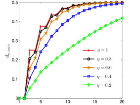
Figure 2: The minimum double-click probability $d_{n,min}$ as a function of the number of photons $n$ arriving at Bob in the active-detection scheme. The results for the mismatch model specified in Table 1 are shown.

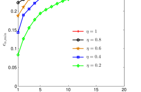
Figure 3: The minimum effective-error probability $e_{n,min}$ as a function of the number of photons $n$ arriving at Bob in the active-detection scheme. The results for the mismatch model specified in Table 1 are shown.

III.2.2 Passive-detection case

In the passive-detection scheme as shown in Fig. 1(b), a 50/50 beam splitter is used for selecting different measurement bases. So, the probability that $n$ incoming photons leave the beam splitter at different output arms is $1-2^{-(n-1)}$, which increases with the photon number $n$. These photons will potentially contribute to clicks at two or more detectors at different output arms of the beam splitter, to which we refer as cross-click events. So, we expect that with the increase of $n$ the cross-click probability conditional on $n$ increases and converges to one. (In contrast, neither the double-click probability nor the effective-error probability increases with $n$, since the probability that $n$ incoming photons leave the beam splitter at the same output arm decreases with $n$.) The above expectation motivates us to consider the following cross-click operator:

$$F_{CC}=I^{A}\otimes M_{CC}^{B},$$ (23)

where $M_{CC}$ is the POVM element for cross-click events at Bob (see Appendix .2 for details of the measurement POVM elements in the passive-detection scheme). Our expectation can be formalized as investigating the following optimization problem:

$$\begin{array}[]{rc}c_{n,min}=&\min_{\rho_{AB}^{(n)}}c_{n}\\ \text{subject to}&\rho_{AB}^{(n)}\geq 0\\ &\operatorname{Tr}\left(\rho_{AB}^{(n)}\right)=1\\ &\left(\rho_{AB}^{(n)}\right)^{\Gamma_{A}}\geq 0,\end{array}$$ (24)

where the objective function is given by $c_{n}=\operatorname{Tr}\left(\rho_{AB}^{(n)}F_{CC}^{(n)}\right)$, and $F_{CC}^{(n)}$ is the projection of the cross-click operator $F_{CC}$ onto the $n$-photons subspace of Bob. The same as in the active-detection case, we constrain the $n$-photons state $\rho_{AB}^{(n)}$ such that it satisfies the PPT criterion.

The above optimization problem is a SDP, which can be solved numerically using the toolbox YALMIP [30] of MATLAB. Strong numerical evidence suggests that with the increase of $n$ the minimum cross-click probability $c_{n,min}$ monotonically increases and converges to one under an arbitrary mismatch model. For the mismatch model specified in Table 2, the optimization results are shown in Fig. 4. As a result, given the observed cross-click probability $c_{\rm{obs}}$, we have that

$$c_{\text{obs}}=\sum_{n=0}^{\infty}p_{n}c_{n}=\sum_{n=2}^{\infty}p_{n}c_{n}\geq\left(1-p_{0}-p_{1}\right)c_{2,min}.$$ (25)

Here, we use the facts that $\sum_{n=0}^{\infty}p_{n}=1$ and $c_{0}=c_{1}=0$. Thus we can bound from below the probability of no more than one photon arriving at Bob.

In the end, we would like to make a comment on the effect of the detection-efficiency mismatch. From Figs. 2, 3 and 4, one can see that, given the photon number $n$, the larger the efficiency mismatch (i.e., the smaller the parameter $\eta$), the smaller the minimum probability of induced double-click events, effective-error events, or cross-click events becomes. In this sense, we expect that the efficiency mismatch helps Eve to attack the QKD system.

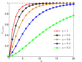
Figure 4: The minimum cross-click probability $c_{n,min}$ as a function of the number of photons $n$ arriving at Bob in the passive-detection scheme. The results for the mismatch model specified in Table 2 are shown.

III.3 Efficiency renormalization

The relative efficiencies of different detectors in Fig. 1 can be those described in Tables 1 and 2. However, in practice no detector has an absolute efficiency $1$. Suppose that the efficiencies of the two detectors in the active-detection scheme of Fig. 1(a) can be written as $\eta_{0}\eta_{1}$ and $\eta_{0}\eta_{2}$ respectively, where $0\leq\eta_{0},\eta_{1},\eta_{2}\leq 1$. Then, there are two equivalent descriptions of the same measurement device, as shown in Fig. 5. According to the description in Fig. 5(b), we can lump together the common loss $\eta_{0}$ in the two detectors and the transmission loss in order to verify entanglement. The reason is as follows: Once entanglement is verified in the state shared between Alice and Bob after passing the beam splitter in Fig. 5(b), then the state before entering the whole measurement device in Fig. 5(a) must be entangled (otherwise, there is contradiction).

According to Fig. 5(b), the detection efficiencies $\eta_{H/D}$ and $\eta_{V/A}$ in measurement POVM elements, such as those in Eqs. (6) and (8), are rescaled by a factor $1/\eta_{0}$. As we observed, given the photon number $n$ arriving at Bob, with the increase of these detection efficiencies both the minimum double-click probability $d_{n,min}$ and the minimum effective-error probability $e_{n,min}$ increase. Hence, given experimental observations, by rescaling detection efficiencies the expectation values of ideal operators in the ($\leq 2$)-photons subspace can be bounded more tightly. We observed that more entangled states can be verified in this way than according to the description in Fig. 5(a). Therefore, in implementations of our method we renormalize detection efficiencies so that the maximum relative efficiency is $1$. The same trick can be applied to the passive-detection scheme, as shown in Fig. 6. Note that the renormalization trick can also be applied to the case with multiple spatial modes. But, for this general case we need to renormalize the efficiencies over all detectors and over all spatial modes at the same time.

In a nutshell, our numerical observations show that if we renormalize detection efficiencies so that the maximum relative efficiency over all detectors and over all spatial modes is $1$, then we can verify more entangled states than according to the actual description of the measurement device.

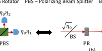
Figure 5: Two equivalent descriptions of the same measurement device in the active-detection scheme, where the detection efficiency is written down around each detector and $0\leq\eta_{0},\eta_{1},\eta_{2}\leq 1$: (a) is the actual situation, and (b) is the hypothetical situation where the common loss $\eta_{0}$ in the two detectors is factored out and treated as a part of transmission loss. The beam splitter in (b) has a transmission coefficient $\sqrt{\eta_{0}}$. See Appendix .4 for a proof of this equivalence.

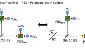
Figure 6: Two equivalent descriptions of the same measurement device in the passive-detection scheme, where the detection efficiency is written down around each detector and $0\leq\eta_{0},\eta_{1},\eta_{2},\eta_{3},\eta_{4}\leq 1$: (a) is the actual situation, and (b) is the hypothetical situation where the common loss $\eta_{0}$ in the four detectors is factored out and treated as a part of transmission loss. The first beam splitter in (b) has a transmission coefficient $\sqrt{\eta_{0}}$. See Appendix .5 for a proof of this equivalence.

III.4 SDP for entanglement verification

According to Observation 1, we can formulate entanglement verification as a SDP problem. Specifically, we need to solve a SDP feasibility problem of the form

$$\begin{array}[]{rc}\text{find}&\chi\\ \text{subject to}&\chi\geq 0\text{ and }\chi^{\Gamma_{A}}\geq 0\\ &\sum_{ijkl}C^{(n)}_{ij,kl}\chi_{ij,kl}=0,n=1,2,...,N\\ &\sum_{ijkl}C^{(m)}_{ij,kl}\chi_{ij,kl}\geq 0,m=N+1,2,...,N+M.\end{array}$$ (26)

Here, the matrix $\chi$ is an EVM, the coefficients $C^{(n)}_{ij,kl}$ with $n=1,2,...,N+M$ are complex numbers, and $N$ and $M$ are the numbers of equality and inequality constraints respectively. The equality constraints can be according to experimental observations and commutation relationships between operators (such as those in Eq. (56) of Appendix .3). The inequality constraints can be derived from operator relationships, such as those in Eqs. (7) and (12), or based on the inequalities in Eqs. (21), (22), and  (25). If the SDP problem in Eq. (26) is not feasible, then the underlying state shared by Alice and Bob must be entangled. In our implementation, the optimization problem in Eq. (26) is solved using the toolbox YALMIP [30] of MATLAB. More details on the formulation of the SDP problem can be found in Appendix .6.

IV Demonstration with simulated results

The method discussed in Sect. III works for general detection-efficiency mismatch models. To illustrate our method, we consider particular mismatch models, such as those specified in Tables 1 and 2. In the absence of a real experiment and for simplicity, we simulate experimental results according to a toy model detailed in the following subsection. We would like to stress that our method for verifying entanglement depends only on experimental observations and measurement POVMs but does not depend on the details of data simulation listed below.

IV.1 Data simulation

We consider the ideal BB84-QKD protocol. Alice first prepares an entangled state as in Eq. (5) according to the source-replacement description. Then Alice sends out the polarized photon to Bob. We model the channel connecting Alice and Bob as a depolarizing channel with depolarizing probability $\omega$; additionally, the transmission loss (i.e., the single-photon loss probability) over the channel is $r$; and Eve intercepts the single photon and resends multiple photons to Bob with probability $p$. The multi-photon state resent by Eve is a randomly-polarized $n$-photons state of the form

$$\rho_{n}=\frac{1}{2n\pi}\int_{0}^{2\pi}\mathrm{d}\theta\left(\hat{a}_{\theta}^{\dagger}\right)^{n}\ket{0}\bra{0}\left(\hat{a}_{\theta}\right)^{n}.$$ (27)

Here, $\hat{a}_{\theta}^{\dagger}=\cos(\theta)\hat{a}_{H}^{\dagger}+\sin(\theta)\hat{a}_{V}^{\dagger}$, and $\hat{a}_{H}^{\dagger}$ (or $\hat{a}_{V}^{\dagger}$) is the creation operator associated with the horizontally-polarized (or vertically-polarized) optical mode. The number of photons $n$ resent will be specified later for each simulation. Moreover, when there is more than one spatial mode, the optical signal is distributed over these spatial modes uniformly randomly. For measurements at Bob, we consider both the active- and passive-detection schemes, as shown in Fig. 1.

IV.2 No-mismatch case and comparison with squashing models

When there is no efficiency mismatch between threshold detectors involved in the measurement device, one can verify entanglement based on squashing models [28, 29, 31, 32]. In this case, Bob uniformly randomly assigns a double-click event to one of the two single-click events at the same measurement basis, and assigns all cross-click events to no detection. Then, his observations can be thought of as generated by a qutrit system (constituted by a single photon and the vacuum). Once we can verify that this qutrit system is entangled with Alice’s system, then the original system shared by Alice and Bob must be entangled [28, 31]. Note that it is still an open question whether or not a squashing model exists in the case of efficiency mismatch.

We compare our method with the one based on squashing models when there is no efficiency mismatch. For this purpose, we simulate experimental results according to the toy model specified in Sec. IV.1. Particularly, we consider the case with no transmission loss. The comparison shows different behaviour, depending on the observations of Alice and Bob. To demonstrate the advantage of our method, we consider the case that the multi-photon state resent by Eve is of the form as in Eq. (27) with $n=2$. (Note that the advantage of our method reduces with the increase of $n$ and finally disappears.) To construct an EVM, we use both the measurement POVM elements (Eq. (9) for the active-detection scheme or Eq. (35) in Appendix .1.2 for the passive-detection scheme) and the ideal operators in the ($\leq 2$)-photons subspace (Eqs. (13), (14) and (15)). The results in Fig. 7 demonstrate the advantage of our method for entanglement verification in the passive-detection scheme. This could be understood as follows: According to the squashing model we discard cross-click events, whereas in our method we take advantage of them in order to bound the number of photons arriving at Bob (see Eq. (25)). Fig. 7 also shows that when there is no mismatch the passive-detection scheme is better for verifying entanglement than the active-detection scheme. This is because the probability of detecting multi-photon events in the passive-detection scheme is higher than that in the active-detection scheme, given the same incoming multi-photon state. So, in the passive-detection scheme our method can take more advantage of operators in the $(\leq 2)$-photons subspace.

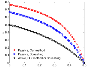
Figure 7: Comparison of our method with the one based on squashing models when there is no efficiency mismatch and no transmission loss. Here, $\omega$ is the depolarizing probability and $p$ is the multi-photon probability in the channel. Below the curves entanglement can be verified. For the active-detection scheme, the results according to our method or based on the squashing model coincide with each other, as shown by diamonds. For the passive-detection scheme, the results according to our method are shown by circles, whereas the results based on the squashing model are shown by squares.

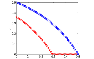
Figure 8: Comparison of the results using EVMs constructed with different numbers of operators in the active-detection scheme. Here, $\omega$ is the depolarizing probability and $p$ is the multi-photon probability in the channel. Below the curves entanglement can be verified. The circles show the results when using only the measurement POVM elements (Eq. (9)) to construct an EVM, whereas the squares show the results when using both the measurement POVM elements (Eq. (9)) and the ideal operators in the ($\leq 2$)-photons subspace (Eqs. (13), (14) and (15)) to construct an EVM. Here, we consider the case with no efficiency mismatch and no transmission loss.

We also observe that it is useful to consider operators in various photon-number subspaces, as demonstrated in Fig. 8. In general, the higher the number of considered photon-number subspaces, the stronger the entanglement-verification power of our method becomes. But, with the increase of the number of considered photon-number subspaces the complexity of the resulting SDP problem increases.

IV.3 Spatial-mode-independent mismatch

Let us start by considering the simple case where the efficiencies of various detectors involved can take different values, but the efficiencies are equal for every spatial mode. Without loss of generality, we assume that there is only one spatial mode. To construct an EVM, we use both the measurement POVM elements (Eq. (9) for the active-detection scheme or Eq. (35) in Appendix .1.2 for the passive-detection scheme) and the ideal operators in the ($\leq 2$)-photons subspace (Eqs. (13), (14) and (15)). The results presented in this subsection are based on simulations according to the toy model specified in Sec. IV.1. For simplicity, we assume that the multi-photon state resent by Eve is of the form as in Eq. (27) with $n\rightarrow\infty$.

First, we compare the abilities of verifying entanglement of the two detection schemes in Fig. 1, when efficiency mismatch is the same. Since there are two detectors in the active-detection scheme, up to permutation symmetry and efficiency renormalization as discussed in Sect. III.3, there is only one kind of mismatch model. Hence, for the purpose of comparison, we consider the case $\eta_{H/D}=1$ and $\eta_{V/A}=\eta<1$ in the active-detection scheme, corresponding to the case $\eta_{H}=\eta_{D}=1$ and $\eta_{V}=\eta_{A}=\eta<1$ in the passive-detection scheme. We would like to find out the minimum efficiency $\eta_{min}$ (corresponding to the maximum mismatch) such that entanglement can be verified as long as $\eta\geq\eta_{min}$. This minimum efficiency $\eta_{min}$ characterizes the robustness of a detection scheme against mismatch for verifying entanglement. Typical results are shown in Fig. 9, where we fix the multi-photon probability $p$ and the transmission loss $r$, and characterize the minimum efficiency $\eta_{min}$ as a function of the depolarizing probability $\omega$. From Fig. 9, one can see that the minimum efficiencies in the active- and passive-detection schemes cross over with each other: For most values of $\omega$ the active-detection scheme is better than the passive-detection scheme in terms of robustness against mismatch. However, there are regions for the values of $\omega$ where the passive-detection scheme is better. Fig. 9 also shows that our method works well even for high-loss cases.

When there are no multi-photon events, i.e., $p=0$, our method can verify entanglement as long as the depolarizing probability satisfies $\omega<1/2$, regardless of the values for the detection efficiency $\eta$ and transmission loss $r$. This is because when $p=0$ our method can certify that there is no more than one photon arriving at Bob. Then, given the observed probability distribution and the mismatch model, the probability distribution for the no-mismatch case can be inferred. In the case of no mismatch, entanglement can be verified as long as the quantum bit error rate is less than $25\%$ [33], which corresponds to the condition that the depolarizing probability satisfies $\omega<1/2$.

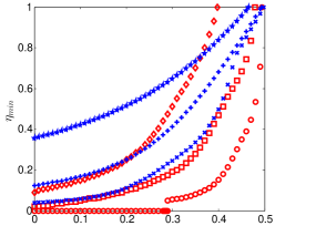
Figure 9: Minimum efficiency $\eta_{min}$ required for verifying entanglement as a function of the depolarizing probability $\omega$ in the channel. The circles, squares and diamonds show the results for the active-detection scheme with transmission losses $r=0,0.75$ and $0.95$, respectively. The crosses, pluses and pentagrams show the results for the passive-detection scheme with transmission losses $r=0,0.75$ and $0.95$, respectively. Here, we fix the multi-photon probability $p=0.01$. We choose the above values of $r$ and $p$ just for ease of graphical illustrations.

Second, we study more general mismatch models in the passive-detection scheme. In this scheme, the efficiencies of the four detectors as shown in Fig. 1(b) can take different values from each other. When fixing the efficiencies of two of the four detectors, for example, $\eta_{H}$ and $\eta_{D}$, there is a trade-off between the efficiencies of the other two detectors, $\eta_{V}$ and $\eta_{A}$, in order to verify entanglement, as shown in Fig. 10.

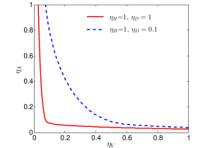
Figure 10: Trade-off between efficiencies $\eta_{V}$ and $\eta_{A}$ under fixed values for $\eta_{H}$ and $\eta_{D}$ in the passive-detection scheme. When the point $(\eta_{V},\eta_{A})$ is above the curve, entanglement can be verified by our method. Here, we fix the depolarizing probability $\omega=0.05$, the multi-photon probability $p=0.01$, and the transmission loss $r=0.5$. We choose these values just for ease of graphical illustrations.

IV.4 Spatial-mode-dependent mismatch

We now increase the number of spatial modes and consider spatial-mode-dependent mismatch models, such as those in Tables 1 and 2. The results presented in this subsection are based on simulations according to the toy model specified in Sec. IV.1. As in the previous subsection, we assume that the multi-photon state resent by Eve is of the form as in Eq. (27) with $n\rightarrow\infty$.

First, let us study the mismatch model in Table 1 for the active-detection scheme. As in the previous subsection, we would like to find out the minimum efficiency $\eta_{min}$ characterizing the robustness of a detection scheme against mismatch for verifying entanglement. Here, we use both measurement POVM elements and the ideal operators in the ($\leq 2$)-photons subspace to construct an EVM (see Appendix .1.1 for details). When there is no transmission loss, i.e., $r=0$, the results are shown in Fig. 11. From this figure, one can see that the higher the depolarizing probability $\omega$ or the multi-photon probability $p$, the larger the minimum efficiency $\eta_{min}$ becomes for verifying entanglement. We also study the effect of transmission loss on entanglement verification, as shown in Fig. 12. From this figure, one can see that our method works well even for high-loss cases. The results in Figs. 11 and 12 suggest that the larger the efficiency mismatch (i.e., the smaller the efficiency $\eta$), the smaller the set of noise parameters $\omega$, $p$ and $r$ that preserve entanglement becomes.

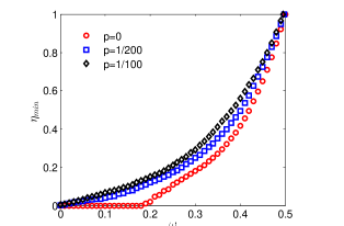
Figure 11: Minimum efficiency $\eta_{min}$ required for verifying entanglement as a function of the depolarizing probability $\omega$ in the channel without transmission loss. Different markers are for different multi-photon probabilities $p$ as labelled in the plot. Here we consider the active-detection scheme. The mismatch model studied is shown in Table 1. We choose the above values of $p$ just for ease of graphical illustrations.

Second, we study the mismatch model in Table 2 for the passive-detection scheme. Here, we use both measurement POVM elements and the ideal operators in the ($\leq 1$)-photon subspace to construct an EVM. Because of the implementation complexity, we do not consider the operators in the two-photons subspace (see Appendix .1.2 for details). The results with or without transmission loss are shown in Figs. 13 and 14, respectively. These results also suggest that the larger the efficiency mismatch (i.e., the smaller the efficiency $\eta$), the smaller the set of noise parameters $\omega$, $p$ and $r$ that preserve entanglement becomes.

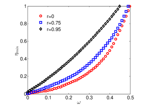
Figure 12: Minimum efficiency $\eta_{min}$ required for verifying entanglement as a function of the depolarizing probability $\omega$ in the channel with transmission loss. Different markers are for different transmission losses $r$ as labelled in the plot. Here we consider the active-detection scheme and fix the multi-photon probability $p=1/200$. The mismatch model studied is shown in Table 1. We choose the above values of $r$ and $p$ just for ease of graphical illustrations.

Note that we cannot compare the robustness of the two detection schemes against mismatch for verifying entanglement via Figs. 11 and 13 or via Figs.12 and 14. The reasons are as follows: First, the mismatch models studied in Tables 1 and 2, for the active- and passive-detection schemes respectively, are different. There is no one-to-one correspondence between these two mismatch models. Second, the EVMs for different detection schemes are constructed using different sets of operators. For the active-detection scheme we use the ideal operators in the ($\leq 2$)-photons subspace, whereas for the passive-detection scheme we use the ideal operators only in the ($\leq 1$)-photon subspace. The higher the number of considered photon-number subspaces, the stronger the entanglement-verification power of our method becomes. Hence, the comparison of the two detection schemes via Figs. 11 and 13 or via Figs. 12 and 14 would not be fair. We would like to stress that we have developed a general method for verifying entanglement with efficiency mismatch. How to optimize our method and improve its entanglement-verification power will require future study.

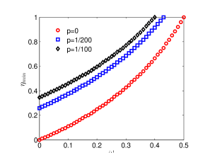
Figure 13: Minimum efficiency $\eta_{min}$ required for verifying entanglement as a function of the depolarizing probability $\omega$ in the channel without transmission loss. Different markers are for different multi-photon probabilities $p$ as labelled in the plot. Here we consider the passive-detection scheme. The mismatch model studied is shown in Table 2. We choose the above values of $p$ just for ease of graphical illustrations.

In the end, we would like to make two notes. First, numerical results suggest that when there are no multi-photon events the ability of our method to verify entanglement does not depend on transmission loss. (The results without multi-photon events and without transmission loss are shown in Figs. 11 and 13, for the active- and passive-detection schemes respectively.) Second, we studied the efficiency mismatch in the experiment of Ref. [26]. As Ref. [26] demonstrated, not only is efficiency mismatched between the four detectors used in the passive-detection scheme, but also the mismatch depends on which one of the four spatial modes contains the incoming optical signal. Ref. [26] studied two different cases, i.e., with or without a pinhole inserting in front of the measurement device. When there is no pinhole, the observed mismatch, as shown in Table 3, is so large that successful intercept-resend attacks on the QKD system exist [26]. When there is a pinhole, the observed mismatch, as shown in Table 4, is reduced so that our method can be used to verify entanglement.

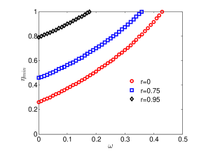
Figure 14: Minimum efficiency $\eta_{min}$ required for verifying entanglement as a function of the depolarizing probability $\omega$ in the channel with transmission loss. Different markers are for different transmission losses $r$ as labelled in the plot. Here we consider the passive-detection scheme and fix the multi-photon probability $p=1/200$. The mismatch model studied is shown in Table 2. We choose the above values of $r$ and $p$ just for ease of graphical illustrations.

Table 3: Spatial-mode-dependent mismatch observed in Ref. [26], when there is no pinhole. Different columns are for different detectors labelled and shown in Fig. 1(b). Different rows are mismatched efficiencies for different spatial modes.

	Det. ‘$H$’	Det. ‘$V$’	Det. ‘$D$’	Det. ‘$A$’
Mode 1	0.08	0	0.00106	0.00106
Mode 2	0	0.0008	0.0001	0.0001
Mode 3	0.002	0.002	0.16	0
Mode 4	0.002	0.002	0	0.04

Table 4: Spatial-mode-dependent mismatch observed in Ref. [26], when there is a pinhole. Different columns are for different detectors labelled and shown in Fig. 1(b). Different rows are mismatched efficiencies for different spatial modes.

	Det. ‘$H$’	Det. ‘$V$’	Det. ‘$D$’	Det. ‘$A$’
Mode 1	0.0004	0	0.0002	0.0002
Mode 2	0	0.0004	0.00033	0.00033
Mode 3	0.0002	0.0002	0.0004	0
Mode 4	0.00033	0.00033	0	0.0004

V Conclusion

Many methods for verifying entanglement assume that various detectors involved in an experimental setup have the same efficiency and that the dimension of the quantum system is fixed and known. However, in practice, the efficiencies of detectors involved in a setup usually do not take the same value, and the tested optical system is not well characterized. To address these problems, one can apply device-independent criteria, such as violations of Bell inequalities. However, these device-independent methods are not robust against transmission loss. Hence, they cannot verify many entangled states that appear in practice. Here, we present a method for verifying entanglement when the efficiency mismatch is characterized. Our method works without the knowledge of the system dimension. The method exploits relationships between measurement POVM elements, particularly those relationships between the projections of measurement POVM elements onto the subspace that contains only a few of photons. The projections contain efficiency-mismatch information, and their expectation values are connected with experimental observations by inequalities. Hence, our method can take advantage of efficiency-mismatch information to verify entanglement.

We implement the method by exploiting the projections of measurement POVM elements onto the ($\leq 2$)-photons subspace. We expect that the entanglement-verification power of our method becomes stronger if a higher-photon-number subspace is considered. We demonstrate our method with simulations. The results show that our method can verify entanglement even if there exists spatial-mode-dependent mismatch, which could be induced by an adversary in the QKD scenario. Moreover, the results show that our method is robust against transmission loss, particularly when the projections of measurement POVM elements onto the two-photons subspace are exploited. For the no-mismatch case, there is another method for verifying entanglement based on squashing models [28, 29]. This method also does not require any system-dimension information. The simulation results show that our method can improve in some cases over squashing models for verifying entanglement (see Fig. 7).

We have addressed the problem of verifying entanglement with efficiency mismatch even without knowing the dimension of the system. Future work is required to adapt the method to prove the security of QKD protocols with efficiency mismatch. It is also desirable to have an analytical proof of the monotonic behaviours of the double-click, effective-error, or cross-click probabilities as functions of the number of photons arriving at Bob, as demonstrated in Figs. 2, 3, and 4. These monotonic behaviours are important for taking advantage of operators in the subspace that contains only a few of photons.

Appendix

.1 Operators exploited for constructing EVMs

In the main text, we discuss only the operators exploited in the case of the active-detection scheme with one spatial mode. Here, we will study other cases considered in the paper.

.1.1 Active-detection scheme with two spatial modes

The idea behind constructing EVMs with two spatial modes (e.g., for the case of the mismatch model in Table 1) is the same as that with one spatial mode studied in Sects. III.1.1 and III.1.2 of the main text. We consider both measurement POVM elements and ideal operators in the $(\leq 2)$-photons subspace for constructing an EVM. However, moving on to the two-spatial-modes case, measurement POVMs change their expressions. Also, more ideal operators in the $(\leq 2)$-photons subspace can be exploited. Let us discuss them in detail.

First, considering the tensor-product structure over the two spatial modes, the expressions of measurement POVM elements change. For example, as long as there is a single click in one of the two spatial modes, it will contribute to the corresponding single-click event in experimental observations. So, the POVM elements for the single-click events in the $H/V$ basis are

$$M_{SC}=M_{SC,1}\otimes M_{\emptyset,2}^{+}+M_{\emptyset,1}^{+}\otimes M_{SC,2}+M_{SC,1}\otimes M_{SC,2},$$ (28)

where the subscript ‘$SC$’ can be either ‘$H$’ or ‘$V$’, and the subscripts ‘1’ and ‘2’ denote the two different spatial modes. For each spatial mode $i$, $i=1$, $2$, the expressions of $M_{H,i},M_{V,i}$ and $M_{\emptyset,i}^{+}$ are the same as those in Eq. (6) with the replacement of detection efficiencies $\eta_{H/D}$ and $\eta_{V/A}$ by those efficiencies $\eta_{H/D,i}$ and $\eta_{V/A,i}$ for the spatial mode $i$. In a similar way, we can write down the other four POVM elements $M_{D}$, $M_{A}$, $M_{HV}$ and $M_{DA}$ required for constructing an EVM. Note that the measurement device cannot measure a photon in a basis that involves a superposition of different spatial modes. So, measurement POVM elements such as those in Eq. (28) are block-diagonal with respect to various photon-number subspaces where the number of photons in each spatial mode is specified.

Second, as for the one-spatial-mode case, the projections of POVM elements onto the zero-photon, one-photon, or two-photons subspaces are linear combinations of ideal operators in these subspaces. The projection onto the zero-photon subspace is still expressed by the ideal operator in the set $\mathbf{\mathcal{S}}_{0}$ of Eq. (13). However, to express the projections onto the one-photon and two-photons subspaces, we need additional ideal operators. For the one-photon case, a photon can either lie in the spatial mode 1 or 2. So the set of ideal operators considered in Eq. (14) expands to two parallel sets

$$\mathbf{\mathcal{S}}_{1,1}\equiv\{I_{2\times 2,1},\tilde{M}_{H,1}^{(1)},\tilde{M}_{D,1}^{(1)},\sigma_{y,1}\}\otimes\Ket{\rm{Vac}}_{2}\Bra{\rm{Vac}}$$ (29)

and

$$\mathbf{\mathcal{S}}_{1,2}\equiv\Ket{\rm{Vac}}_{1}\Bra{\rm{Vac}}\otimes\{I_{2\times 2,2},\tilde{M}_{H,2}^{(1)},\tilde{M}_{D,2}^{(1)},\sigma_{y,2}\},$$ (30)

where the second subscripts ‘1’ and ‘2’ denote the two spatial modes. Note that in Eqs. (29) and (30), the ideal operators for each spatial mode have the same expressions as those for the one-spatial-mode case; the same is true for the ideal operators in the equations below. For the two-photons case, there are three possibilities: Both photons are in the same spatial mode 1 or 2, and one photon is in the spatial mode 1 and the other is in the spatial mode 2. For each of the first two possibilities, the set of ideal operators as defined in Eq. (15) becomes

$$\mathbf{\mathcal{S}}_{2,1}\equiv \{I_{3\times 3,1},\tilde{M}_{H,1}^{(2)},\tilde{M}_{V,1}^{(2)},\tilde{M}_{D,1}^{(2)},\tilde{M}_{A,1}^{(2)},S_{y,1}\}$$

$$\otimes\Ket{\rm{Vac}}_{2}\Bra{\rm{Vac}}$$ (31)

or

$$\mathbf{\mathcal{S}}_{2,2}\equiv \Ket{\rm{Vac}}_{1}\Bra{\rm{Vac}}\otimes$$

$$\{I_{3\times 3,2},\tilde{M}_{H,2}^{(2)},\tilde{M}_{V,2}^{(2)},\tilde{M}_{D,2}^{(2)},\tilde{M}_{A,2}^{(2)},S_{y,2}\}.$$ (32)

For the case that each spatial mode holds one photon, each spatial mode is a qubit system. To describe the projections of measurement POVMs onto this subspace and also to study their operator relationships, we need to consider the following set of ideal operators:

$$\mathbf{\mathcal{S}}_{2,1+2}\equiv\{I_{2\times 2,1}\otimes I_{2\times 2,2},\tilde{M}_{H,1}^{(1)}\otimes I_{2\times 2,2},\tilde{M}_{D,1}^{(1)}\otimes I_{2\times 2,2},$$

$$\sigma_{y,1}\otimes I_{2\times 2,2},I_{2\times 2,1}\otimes\tilde{M}_{H,2}^{(1)},I_{2\times 2,1}\otimes\tilde{M}_{D,2}^{(1)},I_{2\times 2,1}\otimes\sigma_{y,2}\}.$$ (33)

Moreover, in order to exploit the ideal operators within the sets $\mathbf{\mathcal{S}}_{0}$, $\mathbf{\mathcal{S}}_{1,1}$, $\mathbf{\mathcal{S}}_{1,2}$, $\mathbf{\mathcal{S}}_{2,1}$, $\mathbf{\mathcal{S}}_{2,2}$, and $\mathbf{\mathcal{S}}_{2,1+2}$, we need to know the relations between these ideal operators and measurement POVM elements. Once we know the relations, we can bound expectation values of these ideal operators based on experimental observations. As in the one-spatial-mode case, the idea is to express the projections of measurement POVM elements onto the ($\leq 2$)-photons subspace as linear combinations of these ideal operators. Considering the block-diagonal structure of measurement POVM elements with respect to various photon-number subspaces across the two spatial modes, then the relations are established. Therefore, to construct an EVM, we exploit both the measurement operators in the set $\mathbf{\mathcal{S}}$ of Eq. (9) and the ideal operators in the sets $\mathbf{\mathcal{S}}_{0}$ of Eq. (13), $\mathbf{\mathcal{S}}_{1,1}$ of Eq. (29), $\mathbf{\mathcal{S}}_{1,2}$ of Eq. (30), $\mathbf{\mathcal{S}}_{2,1}$ of Eq. (31), $\mathbf{\mathcal{S}}_{2,2}$ of Eq. (32), and $\mathbf{\mathcal{S}}_{2,1+2}$ of Eq. (33).

Note that the constructed EVM can be restricted further by considering the relationships between operators in the above sets. The relationships between the measurement operators in the set $\mathbf{\mathcal{S}}$ are the same as those discussed in Sect. III.1.1 of the main text, even though the expressions of these operators change. For each of the other operator sets, the relationships between operators therein can be derived from those between Pauli operators or between spin-1 operators (see Appendix .3). Moreover, any two operators from any two different sets of $\mathbf{\mathcal{S}}_{0}$, $\mathbf{\mathcal{S}}_{1,1}$, $\mathbf{\mathcal{S}}_{1,2}$, $\mathbf{\mathcal{S}}_{2,1}$, $\mathbf{\mathcal{S}}_{2,2}$ and $\mathbf{\mathcal{S}}_{2,1+2}$ are orthogonal to each other.

.1.2 Passive-detection scheme

In the passive-detection scheme as shown in Fig. 1(b), there are eight possible detection events in total: No click at any of the four detectors, click at only one of the four detectors (single click), clicks at the two detectors at the same output arm of the beam splitter (double click), and clicks at two or more detectors at different output arms of the beam splitter (cross click).

Let us first consider the operators when there is only one spatial mode, since these operators are building blocks for more general cases. In contrast to the active-detection case, the explicit expressions of measurement POVM elements in the full state space are quite lengthy (see Appendix .2). Denote these POVM elements by $M_{\emptyset}$, $M_{H}$, $M_{V}$, $M_{D}$, $M_{A}$, $M_{HV}$, $M_{DA}$, and $M_{CC}$, where the subscripts indicate measurement outcomes and ‘CC’ means cross click. These operators are positive-semidefinite and block-diagonal with respect to various photon-number subspaces. Furthermore, since all POVM elements have eigenvalues between 0 and 1, they satisfy the following relationships:

$$M_{i}\geq M_{i}M_{i}\geq 0,$$ (34)

where $i$ can be $\emptyset$, $H$, $V$, $D$, $A$, $HV$, $DA$, or $CC$. Considering that $M_{\emptyset}+M_{H}+M_{V}+M_{D}+M_{A}+M_{HV}+M_{DA}+M_{CC}=I$ where $I$ is the identity operator in the full state space, we utilize the operator set

$$\mathbf{\mathcal{S}}\equiv\{I,M_{H},M_{V},M_{HV},M_{D},M_{A},M_{DA},M_{CC}\},$$ (35)

to construct an EVM.

We also consider the projections of the above POVM elements onto the ($\leq 2$)-photons subspace, and exploit relationships between these projections. As in the active-detection case, these projections are linear combinations of ideal operators in the same subspace, where the combination coefficients depend on mismatched efficiencies (see Appendix .2 for more details). These ideal operators include those in the operator sets $\mathbf{\mathcal{S}}_{0}$, $\mathbf{\mathcal{S}}_{1}$ and $\mathbf{\mathcal{S}}_{2}$ in Eqs. (13), (14) and (15). As for the active-detection scheme, we can bound the expectation values of these ideal operators and exploit the relationships between them. Hence, in addition to the measurement operators in the set $\mathbf{\mathcal{S}}$ of Eq. (35) we also utilize the ideal operators in the sets $\mathbf{\mathcal{S}}_{0}$, $\mathbf{\mathcal{S}}_{1}$ and $\mathbf{\mathcal{S}}_{2}$ (Eqs. (13) to (15)) for constructing an EVM.

Next, we consider the four-spatial-modes case (e.g., the case of the mismatch model in Table 2). Considering the tensor-product structure over the four spatial modes, the no-click POVM element is

$$M_{\emptyset}=M_{\emptyset,1}\otimes M_{\emptyset,2}\otimes M_{\emptyset,3}\otimes M_{\emptyset,4},$$ (36)

where the subscripts ‘1’, ‘2’, ‘3’ and ‘4’ are the indices of different spatial modes. Moreover, as long as there is a single click in one of the four spatial modes, it will contribute to the corresponding single-click event in experimental observations. So the single-click POVM elements are

$$M_{SC}=M_{?,1}\otimes M_{?,2}\otimes M_{?,3}\otimes M_{?,4},$$ (37)

where the subscript ‘$SC$’ can be ‘$H$’, ‘$V$’, ‘$D$’ or ‘$A$’, and the notation ‘$?$’ can be either single click ‘$SC$’ or no detection ‘$\emptyset$’ but at least one of $M_{?,1}$, $M_{?,2}$, $M_{?,3}$ and $M_{?,4}$ must be the single-click POVM element for the one-spatial-mode case. In a similar way, we can write down the expressions of $M_{HV}$, $M_{DA}$ and $M_{CC}$. Although measurement POVM elements become more complicated as compared with the one-spatial-mode case, they still satisfy the relationships in Eq. (34).

To construct an EVM, we also consider the projections of measurement POVM elements onto the zero-photon and one-photon subspaces. (Unlike the one-spatial-mode case, we do not consider the projections onto the two-photons subspace due to the complexity of both these operators and their relationships.) To express these projections, we need ideal operators in the zero-photon and one-photon subspaces. For the zero-photon case, the ideal operator needed is in the set $\mathbf{\mathcal{S}}_{0}$ of Eq. (13). For the one-photon case, since the photon can be in any one of the four spatial modes, we need the following sets of ideal operators:

$$\mathbf{\mathcal{S}}_{1,1}\equiv \{I_{2\times 2,1},\tilde{M}_{H,1}^{(1)},\tilde{M}_{D,1}^{(1)},\sigma_{y,1}\}\otimes\Ket{\rm{Vac}}_{2}\Bra{\rm{Vac}}$$

$$\otimes\Ket{\rm{Vac}}_{3}\Bra{\rm{Vac}}\otimes\Ket{\rm{Vac}}_{4}\Bra{\rm{Vac}},$$ (38)

$$\mathbf{\mathcal{S}}_{1,2}\equiv \Ket{\rm{Vac}}_{1}\Bra{\rm{Vac}}\otimes\{I_{2\times 2,2},\tilde{M}_{H,2}^{(1)},\tilde{M}_{D,2}^{(1)},\sigma_{y,2}\}$$

$$\otimes\Ket{\rm{Vac}}_{3}\Bra{\rm{Vac}}\otimes\Ket{\rm{Vac}}_{4}\Bra{\rm{Vac}},$$ (39)

$$\mathbf{\mathcal{S}}_{1,3}\equiv \Ket{\rm{Vac}}_{1}\Bra{\rm{Vac}}\otimes\Ket{\rm{Vac}}_{2}\Bra{\rm{Vac}}$$

$$\otimes\{I_{2\times 2,3},\tilde{M}_{H,3}^{(1)},\tilde{M}_{D,3}^{(1)},\sigma_{y,3}\}\otimes\Ket{\rm{Vac}}_{4}\Bra{\rm{Vac}},$$ (40)

and

$$\mathbf{\mathcal{S}}_{1,4}\equiv \Ket{\rm{Vac}}_{1}\Bra{\rm{Vac}}\otimes\Ket{\rm{Vac}}_{2}\Bra{\rm{Vac}}$$

$$\otimes\Ket{\rm{Vac}}_{3}\Bra{\rm{Vac}}\otimes\{I_{2\times 2,4},\tilde{M}_{H,4}^{(1)},\tilde{M}_{D,4}^{(1)},\sigma_{y,4}\}.$$ (41)

The relationships between operators in each of the above sets can be derived from those between Pauli operators (see Appendix .3), while any two operators from any two different sets of $\mathbf{\mathcal{S}}_{0}$, $\mathbf{\mathcal{S}}_{1,1}$, $\mathbf{\mathcal{S}}_{1,2}$, $\mathbf{\mathcal{S}}_{1,3}$ and $\mathbf{\mathcal{S}}_{1,4}$ are orthogonal to each other. Moreover, as for the active-detection scheme, we can bound the expectation values of these ideal operators based on experimental observations. Therefore, to construct an EVM for the four-spatial-modes case, we utilize not only the measurement operators in the set $\mathbf{\mathcal{S}}$ of Eq. (35) but also the ideal operators in the sets $\mathbf{\mathcal{S}}_{0}$ of Eq. (13), $\mathbf{\mathcal{S}}_{1,1}$ of Eq. (38), $\mathbf{\mathcal{S}}_{1,2}$ of Eq. (39), $\mathbf{\mathcal{S}}_{1,3}$ of Eq. (40) and $\mathbf{\mathcal{S}}_{1,4}$ of Eq. (41).

.2 POVM elements with mismatched efficiencies

We first consider the active-detection scheme as shown in Fig. 1(a). Suppose that the two threshold detectors have efficiencies $\eta_{H/D}$ and $\eta_{V/A}$, respectively. Recall that a real threshold detector can be described by an ideal threshold detector with a beam splitter in front whose transmission coefficient is equal to the square root of the real detector’s efficiency [34]. It then turns out that the measurement in the $H/V$ basis can be described by an optical device with three input spatial directions labelled by numbers and four output spatial directions labelled by lower-case letters, as shown in Fig. 15. In order to realize the measurement, however, only the input spatial direction 1 has incoming optical signals, whereas no signals travel along the other two input spatial directions 2 and 3. To get an outcome, the output modes $H_{a}$ and $V_{c}$ are measured with ideal threshold detectors, whereas the other two output modes $H_{b}$ and $V_{d}$ are not detected corresponding to the loss in the measurement process. (Note that here and later we use both the polarization degree of freedom and the spatial degree of freedom to label an input or output mode.) Therefore, it is straightforward to write down POVM elements in the output-modes basis $\{\Ket{n_{H_{a}},n_{H_{b}},n_{V_{c}},n_{V_{d}}},n_{H_{a}},n_{H_{b}},n_{V_{c}},n_{V_{d}}=0,1,2,...\}$. For example, the POVM element for the single-click event ‘$H$’ is written as

$$M_{H}= \sum_{n_{H_{a}}=1}^{\infty}\sum_{n_{H_{b}}=0}^{\infty}\sum_{n_{V_{d}}=0}^{\infty}$$

$$\Ket{n_{H_{a}},n_{H_{b}},0_{V_{c}},n_{V_{d}}}\Bra{n_{H_{a}},n_{H_{b}},0_{V_{c}},n_{V_{d}}}.$$ (42)

Using the fact $\Ket{n}=\frac{1}{\sqrt{n!}}(\hat{a}^{\dagger})^{n}\Ket{0}$, Eq. (42) becomes

$$M_{H}= \sum_{n_{H_{a}}=1}^{\infty}\sum_{n_{H_{b}}=0}^{\infty}\sum_{n_{V_{d}}=0}^{\infty}\frac{1}{n_{H_{a}}!\,n_{H_{b}}!\,n_{V_{d}}!}$$

$$\left(\hat{a}_{H_{a}}^{\dagger}\right)^{n_{H_{a}}}\left(\hat{a}_{H_{b}}^{\dagger}\right)^{n_{H_{b}}}\left(\hat{a}_{V_{d}}^{\dagger}\right)^{n_{V_{d}}}\Ket{0}\Bra{0}$$

$$\left(\hat{a}_{H_{a}}\right)^{n_{H_{a}}}\left(\hat{a}_{H_{b}}\right)^{n_{H_{b}}}\left(\hat{a}_{V_{d}}\right)^{n_{V_{d}}},$$ (43)

where $\hat{a}$ and $\hat{a}^{\dagger}$ are annihilation and creation operators associated with an optical mode, respectively.

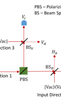
Figure 15: Description of the measurement in the $H/V$ basis under the active-detection scheme. Suppose that the detection efficiencies associated with the outcomes $H$ and $V$ are $\eta_{H/D}$ and $\eta_{V/A}$, respectively, and that the two detectors shown are ideal. Then, the beam splitters BS_H and BS_V have transmission coefficients $\sqrt{\eta_{H/D}}$ and $\sqrt{\eta_{V/A}}$, respectively.

To express the POVM element $M_{H}$ in the input-modes basis, we utilize the relations between the creation operators of the input and output modes of a beam splitter. Specifically, the relations

$$\hat{a}_{H_{a}}^{\dagger}=\sqrt{\eta_{H/D}}\hat{a}_{H_{1}}^{\dagger}+\sqrt{1-\eta_{H/D}}\hat{a}_{H_{2}}^{\dagger},$$

$$\hat{a}_{H_{b}}^{\dagger}=-\sqrt{1-\eta_{H/D}}\hat{a}_{H_{1}}^{\dagger}+\sqrt{\eta_{H/D}}\hat{a}_{H_{2}}^{\dagger},\text{ and}$$

$$\hat{a}_{V_{d}}^{\dagger}=-\sqrt{1-\eta_{V/A}}\hat{a}_{V_{1}}^{\dagger}+\sqrt{\eta_{V/A}}\hat{a}_{V_{3}}^{\dagger}.$$ (44)

Using Eq. (44), we can express $M_{H}$ in terms of the creation operators $\hat{a}_{H_{1}}^{\dagger},\hat{a}_{V_{1}}^{\dagger}$, $\hat{a}_{H_{2}}^{\dagger}$ and $\hat{a}_{V_{3}}^{\dagger}$ and the annihilation operators $\hat{a}_{H_{1}},\hat{a}_{V_{1}},\hat{a}_{H_{2}}$ and $\hat{a}_{V_{3}}$. Further, to fulfill the physical condition that there is no incoming optical signal travelling along the spatial directions 2 or 3, we need to pick only the terms where there is no appearance of any of the operators $\hat{a}_{H_{2}}^{\dagger}$, $\hat{a}_{V_{3}}^{\dagger}$, $\hat{a}_{H_{2}}$, and $\hat{a}_{V_{3}}$. Therefore, we get that

$$M_{H}= \sum_{n_{H_{a}}=1}^{\infty}\sum_{n_{H_{b}}=0}^{\infty}\sum_{n_{V_{d}}=0}^{\infty}\frac{1}{n_{H_{a}}!\,n_{H_{b}}!\,n_{V_{d}}!}$$

$$(\eta_{H/D})^{n_{H_{a}}}(1-\eta_{H/D})^{n_{H_{b}}}(1-\eta_{V/A})^{n_{V_{d}}}\left(\hat{a}_{H_{1}}^{\dagger}\right)^{n_{H_{a}}+n_{H_{b}}}$$

$$\left(\hat{a}_{V_{1}}^{\dagger}\right)^{n_{V_{d}}}\Ket{0}\Bra{0}\left(\hat{a}_{H_{1}}\right)^{n_{H_{a}}+n_{H_{b}}}\left(\hat{a}_{V_{1}}\right)^{n_{V_{d}}}.$$ (45)

Using the fact that $(\hat{a}^{\dagger})^{n}\Ket{0}=\sqrt{n!}\Ket{n}$, and setting that $n_{H_{1}}=n_{H_{a}}+n_{H_{b}}$ and $n_{V_{1}}=n_{V_{d}}$, we can simplify the above equation to

$$M_{H}= \sum_{n_{H_{1}}=1}^{\infty}\sum_{n_{V_{1}}=0}^{\infty}\left(1-(1-\eta_{H/D})^{n_{H_{1}}}\right)(1-\eta_{V/A})^{n_{V_{1}}}$$

$$\Ket{n_{H_{1}},n_{V_{1}}}\Bra{n_{H_{1}},n_{V_{1}}}.$$ (46)

The above equation is the same as that in Eq. (6) of the main text, except that each polarization mode has a subscript ‘1’ indicating the input spatial direction.

Likewise, we can derive the other POVM elements for the measurement in the $H/V$ basis, and the results are as follows:

$$M_{V}= \sum_{n_{H_{1}}=0}^{\infty}\sum_{n_{V_{1}}=1}^{\infty}(1-\eta_{H/D})^{n_{H_{1}}}\left(1-(1-\eta_{V/A})^{n_{V_{1}}}\right)$$

$$\Ket{n_{H_{1}},n_{V_{1}}}\Bra{n_{H_{1}},n_{V_{1}}},$$

$$M_{HV}= \sum_{n_{H_{1}}=1}^{\infty}\sum_{n_{V_{1}}=1}^{\infty}\left(1-(1-\eta_{H/D})^{n_{H_{1}}}\right)\left(1-(1-\eta_{V/A})^{n_{V_{1}}}\right)$$

$$\Ket{n_{H_{1}},n_{V_{1}}}\Bra{n_{H_{1}},n_{V_{1}}},\text{ and}$$

$$M_{\emptyset}^{+}= \sum_{n_{H_{1}}=0}^{\infty}\sum_{n_{V_{1}}=0}^{\infty}(1-\eta_{H/D})^{n_{H_{1}}}(1-\eta_{V/A})^{n_{V_{1}}}$$

$$\Ket{n_{H_{1}},n_{V_{1}}}\Bra{n_{H_{1}},n_{V_{1}}},$$ (47)

where the superscript ‘$+$’ denotes the $H/V$ basis.

Figure 16: Description of the measurement under the passive-detection scheme. Suppose that the detection efficiencies associated with the outcomes $H$, $V$, $D$ and $A$ are $\eta_{H}$, $\eta_{V}$, $\eta_{D}$ and $\eta_{A}$ respectively, and that the four detectors shown are ideal. Then, the beam splitters BS_H, BS_V, BS_D and BS_A have transmission coefficients $\sqrt{\eta_{H}}$, $\sqrt{\eta_{V}}$, $\sqrt{\eta_{D}}$ and $\sqrt{\eta_{A}}$, respectively.

We can follow the same procedure as above to derive the POVM elements for the measurement in the $D/A$ basis under the active-detection scheme. We skip the details and just list the POVM elements as follows:

$$M_{D}= \sum_{n_{D_{1}}=1}^{\infty}\sum_{n_{A_{1}}=0}^{\infty}\left(1-(1-\eta_{H/D})^{n_{D_{1}}}\right)(1-\eta_{V/A})^{n_{A_{1}}}$$

$$\Ket{n_{D_{1}},n_{A_{1}}}\Bra{n_{D_{1}},n_{A_{1}}},$$

$$M_{A}= \sum_{n_{D_{1}}=0}^{\infty}\sum_{n_{A_{1}}=1}^{\infty}(1-\eta_{H/D})^{n_{D_{1}}}\left(1-(1-\eta_{V/A})^{n_{A_{1}}}\right)$$

$$\Ket{n_{D_{1}},n_{A_{1}}}\Bra{n_{D_{1}},n_{A_{1}}},$$

$$M_{DA}= \sum_{n_{D_{1}}=1}^{\infty}\sum_{n_{A_{1}}=1}^{\infty}\left(1-(1-\eta_{H/D})^{n_{D_{1}}}\right)\left(1-(1-\eta_{V/A})^{n_{A_{1}}}\right)$$

$$\Ket{n_{D_{1}},n_{A_{1}}}\Bra{n_{D_{1}},n_{A_{1}}},\text{ and}$$

$$M_{\emptyset}^{\times}= \sum_{n_{D_{1}}=0}^{\infty}\sum_{n_{A_{1}}=0}^{\infty}(1-\eta_{H/D})^{n_{D_{1}}}(1-\eta_{V/A})^{n_{A_{1}}}$$

$$\Ket{n_{D_{1}},n_{A_{1}}}\Bra{n_{D_{1}},n_{A_{1}}}.$$ (48)

Here, the superscript ‘$\times$’ denotes the $D/A$ basis, and the subscript ‘1’ of the polarization mode denotes the input spatial direction.

Next, let us study the passive-detection case. With the help of the beam-splitter model for a real detector with imperfect efficiency, we can see that the whole measurement can be described by an optical device with six input spatial directions and eight output spatial directions, as shown in Fig. 16. To realize the measurement, only the input spatial direction 1 has incoming optical signals, and only the output modes $H_{a}$, $V_{c}$, $D_{e}$ and $A_{g}$ are measured (by ideal detectors). It is straightforward to see that in the output-modes basis $\{\Ket{n_{H_{a}},n_{H_{b}},n_{V_{c}},n_{V_{d}},n_{D_{e}},n_{D_{f}},n_{A_{g}},n_{A_{h}}},n_{H_{a}},n_{H_{b}},n_{V_{c}},\\ n_{V_{d}},n_{D_{e}},n_{D_{f}},n_{A_{g}},n_{A_{h}}=0,1,2,...\}$, the POVM element for the single-click event ‘$H$’ is written as

$$M_{H}= \sum_{n_{H_{a}}=1}^{\infty}\sum_{n_{H_{b}}=0}^{\infty}\sum_{n_{V_{d}}=0}^{\infty}\sum_{n_{D_{f}}=0}^{\infty}\sum_{n_{A_{h}}=0}^{\infty}$$

$$\Ket{n_{H_{a}},n_{H_{b}},0_{V_{c}},n_{V_{d}},0_{D_{e}},n_{D_{f}},0_{A_{g}},n_{A_{h}}}$$

$$\Bra{n_{H_{a}},n_{H_{b}},0_{V_{c}},n_{V_{d}},0_{D_{e}},n_{D_{f}},0_{A_{g}},n_{A_{h}}}.$$ (49)

To express the above POVM element $M_{H}$ in the input-modes basis, as for the active-detection case, we use the fact that $\Ket{n}=\frac{1}{\sqrt{n!}}(\hat{a}^{\dagger})^{n}\Ket{0}$ and the relations between the creation operators of the input and output modes of a beam splitter. Here, we skip the lengthy but not difficult details, and just write down the final expression of $M_{H}$ as follows:

$$M_{H}= \sum_{n_{H_{a}}=1}^{\infty}\sum_{n_{H_{b}}=0}^{\infty}\sum_{n_{V_{d}}=0}^{\infty}\sum_{n_{D_{f}}=0}^{\infty}\sum_{n_{A_{h}}=0}^{\infty}\left(\frac{1}{2}\right)^{n_{H_{a}}+n_{H_{b}}+n_{V_{d}}+n_{D_{f}}+n_{A_{h}}}$$

$$\frac{1}{n_{H_{a}}!\,n_{H_{b}}!\,n_{V_{d}}!\,n_{D_{f}}!\,n_{A_{h}}!}(\eta_{H})^{n_{H_{a}}}(1-\eta_{H})^{n_{H_{b}}}(1-\eta_{V})^{n_{V_{d}}}(1-\eta_{D})^{n_{D_{f}}}(1-\eta_{A})^{n_{A_{h}}}$$

$$\left(\hat{a}_{H_{1}}^{\dagger}\right)^{n_{H_{a}}+n_{H_{b}}}\left(\hat{a}_{V_{1}}^{\dagger}\right)^{n_{V_{d}}}\left(\hat{a}_{D_{1}}^{\dagger}\right)^{n_{D_{f}}}\left(\hat{a}_{A_{1}}^{\dagger}\right)^{n_{A_{h}}}\Ket{0}\Bra{0}\left(\hat{a}_{H_{1}}\right)^{n_{H_{a}}+n_{H_{b}}}\left(\hat{a}_{V_{1}}\right)^{n_{V_{d}}}\left(\hat{a}_{D_{1}}\right)^{n_{D_{f}}}\left(\hat{a}_{A_{1}}\right)^{n_{A_{h}}}.$$ (50)

Likewise, we can get the following results:

$$M_{V}= \sum_{n_{H_{b}}=0}^{\infty}\sum_{n_{V_{c}}=1}^{\infty}\sum_{n_{V_{d}}=0}^{\infty}\sum_{n_{D_{f}}=0}^{\infty}\sum_{n_{A_{h}}=0}^{\infty}\left(\frac{1}{2}\right)^{n_{H_{b}}+n_{V_{c}}+n_{V_{d}}+n_{D_{f}}+n_{A_{h}}}$$

$$\frac{1}{n_{H_{b}}!\,n_{V_{c}}!\,n_{V_{d}}!\,n_{D_{f}}!\,n_{A_{h}}!}(1-\eta_{H})^{n_{H_{b}}}(\eta_{V})^{n_{V_{c}}}(1-\eta_{V})^{n_{V_{d}}}(1-\eta_{D})^{n_{D_{f}}}(1-\eta_{A})^{n_{A_{h}}}$$

$$\left(\hat{a}_{H_{1}}^{\dagger}\right)^{n_{H_{b}}}\left(\hat{a}_{V_{1}}^{\dagger}\right)^{n_{V_{c}}+n_{V_{d}}}\left(\hat{a}_{D_{1}}^{\dagger}\right)^{n_{D_{f}}}\left(\hat{a}_{A_{1}}^{\dagger}\right)^{n_{A_{h}}}\Ket{0}\Bra{0}\left(\hat{a}_{H_{1}}\right)^{n_{H_{b}}}\left(\hat{a}_{V_{1}}\right)^{n_{V_{c}}+n_{V_{d}}}\left(\hat{a}_{D_{1}}\right)^{n_{D_{f}}}\left(\hat{a}_{A_{1}}\right)^{n_{A_{h}}},$$

$$M_{D}= \sum_{n_{H_{b}}=0}^{\infty}\sum_{n_{V_{d}}=0}^{\infty}\sum_{n_{D_{e}}=1}^{\infty}\sum_{n_{D_{f}}=0}^{\infty}\sum_{n_{A_{h}}=0}^{\infty}\left(\frac{1}{2}\right)^{n_{H_{b}}+n_{V_{d}}+n_{D_{e}}+n_{D_{f}}+n_{A_{h}}}$$

$$\frac{1}{n_{H_{b}}!\,n_{V_{d}}!\,n_{D_{e}}!\,n_{D_{f}}!\,n_{A_{h}}!}(1-\eta_{H})^{n_{H_{b}}}(1-\eta_{V})^{n_{V_{d}}}(\eta_{D})^{n_{D_{e}}}(1-\eta_{D})^{n_{D_{f}}}(1-\eta_{A})^{n_{A_{h}}}$$

$$\left(\hat{a}_{H_{1}}^{\dagger}\right)^{n_{H_{b}}}\left(\hat{a}_{V_{1}}^{\dagger}\right)^{n_{V_{d}}}\left(\hat{a}_{D_{1}}^{\dagger}\right)^{n_{D_{e}}+n_{D_{f}}}\left(\hat{a}_{A_{1}}^{\dagger}\right)^{n_{A_{h}}}\Ket{0}\Bra{0}\left(\hat{a}_{H_{1}}\right)^{n_{H_{b}}}\left(\hat{a}_{V_{1}}\right)^{n_{V_{d}}}\left(\hat{a}_{D_{1}}\right)^{n_{D_{e}}+n_{D_{f}}}\left(\hat{a}_{A_{1}}\right)^{n_{A_{h}}},$$

$$M_{A}= \sum_{n_{H_{b}}=0}^{\infty}\sum_{n_{V_{d}}=0}^{\infty}\sum_{n_{D_{f}}=0}^{\infty}\sum_{n_{A_{g}}=1}^{\infty}\sum_{n_{A_{h}}=0}^{\infty}\left(\frac{1}{2}\right)^{n_{H_{b}}+n_{V_{d}}+n_{D_{f}}+n_{A_{g}}+n_{A_{h}}}$$

$$\frac{1}{n_{H_{b}}!\,n_{V_{d}}!\,n_{D_{f}}!\,n_{A_{g}}!\,n_{A_{h}}!}(1-\eta_{H})^{n_{H_{b}}}(1-\eta_{V})^{n_{V_{d}}}(1-\eta_{D})^{n_{D_{f}}}(\eta_{A})^{n_{A_{g}}}(1-\eta_{A})^{n_{A_{h}}}$$

$$\left(\hat{a}_{H_{1}}^{\dagger}\right)^{n_{H_{b}}}\left(\hat{a}_{V_{1}}^{\dagger}\right)^{n_{V_{d}}}\left(\hat{a}_{D_{1}}^{\dagger}\right)^{n_{D_{f}}}\left(\hat{a}_{A_{1}}^{\dagger}\right)^{n_{A_{g}}+n_{A_{h}}}\Ket{0}\Bra{0}\left(\hat{a}_{H_{1}}\right)^{n_{H_{b}}}\left(\hat{a}_{V_{1}}\right)^{n_{V_{d}}}\left(\hat{a}_{D_{1}}\right)^{n_{D_{f}}}\left(\hat{a}_{A_{1}}\right)^{n_{A_{g}}+n_{A_{h}}},$$

$$M_{HV}= \sum_{n_{H_{a}}=1}^{\infty}\sum_{n_{H_{b}}=0}^{\infty}\sum_{n_{V_{c}}=1}^{\infty}\sum_{n_{V_{d}}=0}^{\infty}\sum_{n_{D_{f}}=0}^{\infty}\sum_{n_{A_{h}}=0}^{\infty}\left(\frac{1}{2}\right)^{n_{H_{a}}+n_{H_{b}}+n_{V_{c}}+n_{V_{d}}+n_{D_{f}}+n_{A_{h}}}$$

$$\frac{1}{n_{H_{a}}!\,n_{H_{b}}!\,n_{V_{c}}!\,n_{V_{d}}!\,n_{D_{f}}!\,n_{A_{h}}!}(\eta_{H})^{n_{H_{a}}}(1-\eta_{H})^{n_{H_{b}}}(\eta_{V})^{n_{V_{c}}}(1-\eta_{V})^{n_{V_{d}}}(1-\eta_{D})^{n_{D_{f}}}(1-\eta_{A})^{n_{A_{h}}}$$

$$\left(\hat{a}_{H_{1}}^{\dagger}\right)^{n_{H_{a}}+n_{H_{b}}}\left(\hat{a}_{V_{1}}^{\dagger}\right)^{n_{V_{c}}+n_{V_{d}}}\left(\hat{a}_{D_{1}}^{\dagger}\right)^{n_{D_{f}}}\left(\hat{a}_{A_{1}}^{\dagger}\right)^{n_{A_{h}}}\Ket{0}\Bra{0}\left(\hat{a}_{H_{1}}\right)^{n_{H_{a}}+n_{H_{b}}}\left(\hat{a}_{V_{1}}\right)^{n_{V_{c}}+n_{V_{d}}}\left(\hat{a}_{D_{1}}\right)^{n_{D_{f}}}\left(\hat{a}_{A_{1}}\right)^{n_{A_{h}}},$$

$$M_{DA}= \sum_{n_{H_{b}}=0}^{\infty}\sum_{n_{V_{d}}=0}^{\infty}\sum_{n_{D_{e}}=1}^{\infty}\sum_{n_{D_{f}}=0}^{\infty}\sum_{n_{A_{g}}=1}^{\infty}\sum_{n_{A_{h}}=0}^{\infty}\left(\frac{1}{2}\right)^{n_{H_{b}}+n_{V_{d}}+n_{D_{e}}+n_{D_{f}}+n_{A_{g}}+n_{A_{h}}}$$

$$\frac{1}{n_{H_{b}}!\,n_{V_{d}}!\,n_{D_{e}}!\,n_{D_{f}}!\,n_{A_{g}}!\,n_{A_{h}}!}(1-\eta_{H})^{n_{H_{b}}}(1-\eta_{V})^{n_{V_{d}}}(\eta_{D})^{n_{D_{e}}}(1-\eta_{D})^{n_{D_{f}}}(\eta_{A})^{n_{A_{g}}}(1-\eta_{A})^{n_{A_{h}}}$$

$$\left(\hat{a}_{H_{1}}^{\dagger}\right)^{n_{H_{b}}}\left(\hat{a}_{V_{1}}^{\dagger}\right)^{n_{V_{d}}}\left(\hat{a}_{D_{1}}^{\dagger}\right)^{n_{D_{e}}+n_{D_{f}}}\left(\hat{a}_{A_{1}}^{\dagger}\right)^{n_{A_{g}}+n_{A_{h}}}\Ket{0}\Bra{0}\left(\hat{a}_{H_{1}}\right)^{n_{H_{b}}}\left(\hat{a}_{V_{1}}\right)^{n_{V_{d}}}\left(\hat{a}_{D_{1}}\right)^{n_{D_{e}}+n_{D_{f}}}\left(\hat{a}_{A_{1}}\right)^{n_{A_{g}}+n_{A_{h}}},$$

and

$$M_{\emptyset}= \sum_{n_{H_{b}}=0}^{\infty}\sum_{n_{V_{d}}=0}^{\infty}\sum_{n_{D_{f}}=0}^{\infty}\sum_{n_{A_{h}}=0}^{\infty}\left(\frac{1}{2}\right)^{n_{H_{b}}+n_{V_{d}}+n_{D_{f}}+n_{A_{h}}}$$

$$\frac{1}{n_{H_{b}}!\,n_{V_{d}}!\,n_{D_{f}}!\,n_{A_{h}}!}(1-\eta_{H})^{n_{H_{b}}}(1-\eta_{V})^{n_{V_{d}}}(1-\eta_{D})^{n_{D_{f}}}(1-\eta_{A})^{n_{A_{h}}}\left(\hat{a}_{H_{1}}^{\dagger}\right)^{n_{H_{b}}}\left(\hat{a}_{V_{1}}^{\dagger}\right)^{n_{V_{d}}}$$

$$\left(\hat{a}_{D_{1}}^{\dagger}\right)^{n_{D_{f}}}\left(\hat{a}_{A_{1}}^{\dagger}\right)^{n_{A_{h}}}\Ket{0}\Bra{0}\left(\hat{a}_{H_{1}}\right)^{n_{H_{b}}}\left(\hat{a}_{V_{1}}\right)^{n_{V_{d}}}\left(\hat{a}_{D_{1}}\right)^{n_{D_{f}}}\left(\hat{a}_{A_{1}}\right)^{n_{A_{h}}}.$$ (51)

There is no obvious simplification of Eqs. (50) and (51), but from these expressions it is straightforward to see that the POVM elements are linear combinations of ideal operators where the combination coefficients are determined by the mismatched efficiencies $\eta_{H}$, $\eta_{V}$, $\eta_{D}$ and $\eta_{A}$. Note that we did not write down the POVM element $M_{CC}$ for cross-click events, since it can be inferred from the fact $M_{\emptyset}+M_{H}+M_{V}+M_{D}+M_{A}+M_{HV}+M_{DA}+M_{CC}=I$ where $I$ is the identity operator in the full state space.

.3 Relationships between ideal operators

To figure out the relationships between the ideal operators in Eq. (11), we note that these ideal operators are related to Pauli operators (or spin-$\frac{1}{2}$ operators)

$$\sigma_{x}=\left(\begin{array}[]{c c}0&1\\ 1&0\end{array}\right),\sigma_{y}=\left(\begin{array}[]{c c}0&-i\\ i&0\end{array}\right),\text{ and }\sigma_{z}=\left(\begin{array}[]{c c}1&0\\ 0&-1\end{array}\right),$$ (52)

and spin-1 operators

$$S_{x}=\frac{1}{\sqrt{2}}\left(\begin{array}[]{c c c}0&1&0\\ 1&0&1\\ 0&1&0\end{array}\right),S_{y}=\frac{1}{\sqrt{2}}\left(\begin{array}[]{c c c}0&-i&0\\ i&0&-i\\ 0&i&0\end{array}\right),\text{ and }S_{z}=\left(\begin{array}[]{c c c}1&0&0\\ 0&0&0\\ 0&0&-1\end{array}\right).$$ (53)

Particularly, in the basis $\{\Ket{1_{H},0_{V}},\Ket{0_{H},1_{V}}\}$ of the one-photon subspace we have

$$2\tilde{M}_{H}^{(1)}-I_{2\times 2}=\sigma_{z}\text{ and }2\tilde{M}_{D}^{(1)}-I_{2\times 2}=\sigma_{x},$$ (54)

and in the basis $\{\Ket{2_{H},0_{V}},\Ket{1_{H},1_{V}},\Ket{0_{H},2_{V}}\}$ of the two-photons subspace we have

$$\tilde{M}_{H}^{(2)}-\tilde{M}_{V}^{(2)}=S_{z}\text{ and }\tilde{M}_{D}^{(2)}-\tilde{M}_{A}^{(2)}=S_{x}.$$ (55)

So, we can derive the relationships between the ideal operators in Eq. (11) from those between Pauli operators or between spin-1 operators, for example, from

$$\sigma_{a}\sigma_{b}=i\varepsilon_{abc}\sigma_{c}+\delta_{ab}I_{2\times 2},\text{ or }[S_{a},S_{b}]=i\varepsilon_{abc}S_{c},$$ (56)

where $\varepsilon_{abc}$ is the Levi-Civita symbol, $\delta_{ab}$ is the Kronecker delta function, and each of $a$, $b$ and $c$ can be $x$, $y$ or $z$.

In the same way, we can derive the relationships between the ideal operators in Eqs. (29) to (33) and Eqs. (38) to (41).

.4 Proof of the equivalence of the descriptions in Fig. 5

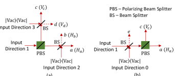
Figure 17: Two equivalent descriptions of the measurement in the $H/V$ basis under the active-detection scheme: (a) is the actual situation (the same as Fig. 5(a)), and (b) is the hypothetical situation (the same as Fig. 5(b)). Suppose that the detection efficiencies associated with the outcomes $H$ and $V$ can be written as $\eta_{0}\eta_{1}$ and $\eta_{0}\eta_{2}$ respectively, where $0\leq\eta_{0},\eta_{1},\eta_{2}\leq 1$. Then, to realize the measurement, each beam splitter as shown has a transmission coefficient $\sqrt{\eta_{0}}$, and the output modes $H_{a}$ and $V_{c}$ are detected by real detectors with efficiencies $\eta_{1}$ and $\eta_{2}$, respectively. The two real detectors are not shown for simplicity. Note that the other output modes $H_{b}$ and $V_{d}$ in (a) and $H_{e}$ and $V_{e}$ in (b) are not detected, corresponding to the loss in the measurement process.

Without loss of generality, we assume that the measurement is performed in the $H/V$ basis. From Appendix .2, we already know the POVM elements for the measurement described in Fig. 5(a), i.e., Eqs. (46) and (47) with the replacement of $\eta_{H/D}$ and $\eta_{V/A}$ by $\eta_{0}\eta_{1}$ and $\eta_{0}\eta_{2}$, respectively. To prove the equivalence, we can derive the POVM elements for the measurement described in Fig. 5(b). However, this approach is quite lengthy. To simplify the proof and make the idea behind clear, we take another approach.

It is straightforward to see that Fig. 5(a) (or Fig. 5(b)) is the same as Fig. 17(a) (or Fig. 17(b)) where only the input spatial direction 1 has incoming optical signals and only the output modes $H_{a}$ and $V_{c}$ are detected (by real detectors with efficiencies $\eta_{1}$ and $\eta_{2}$ respectively). The optical devices in Fig. 17(a) and Fig. 17(b) are equivalent because of the well-known result that the common loss $\eta_{0}$ in the two output arms of a polarizing beam splitter can also be introduced by inserting a beam splitter with a transmission coefficient $\sqrt{\eta_{0}}$ for both polarization modes into the input arm of the polarizing beam splitter.

.5 Proof of the equivalence of the descriptions in Fig. 6

In the passive-detection scheme as shown in Fig. 1(b), each output arm of the $50/50$ beam splitter is a setup for the active-detection scheme, i.e., a polarizing beam splitter with a detector in each output arm of the polarizing beam splitter. From Fig. 17 of Appendix .4, we already see that a common loss in the two output arms of a polarizing beam splitter can be introduced either by inserting a beam splitter into each output arm or by inserting the same beam splitter into the input arm of the polarizing beam splitter. Hence, to prove the equivalence of Fig. 6(a) and Fig. 6(b), we only need to further prove that a common loss in the two output arms of a $50/50$ beam splitter as shown in Fig. 18(a) is equivalent to the same common loss in the two input arms of the $50/50$ beam splitter as shown in Fig. 18(b). This equivalence is well established in quantum optics, so here we skip the proof.

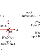
Figure 18: Two equivalent descriptions of a $50/50$ beam splitter with a common loss in the two output arms: (a) is the case where the loss is introduced in each output arm, and (b) is the case where the loss is introduced in each input arm. Suppose that the common loss is $\eta_{0}$. Then, each beam splitter as shown has a transmission coefficient $\sqrt{\eta_{0}}$. The whole optical device in each case has four input spatial directions and four output spatial directions.

.6 Details of the SDP problem

In Sect. III.4 of the main text, we formulate entanglement verification as a SDP feasibility problem of the form in Eq. (26). Here we provide more details of the SDP problem to be solved for the case of the active-detection scheme with one spatial mode. The SDP problems for the other cases studied in the paper can be formulated in the same way.

For the ideal BB84-QKD prepare-and-measure protocol studied in Sect. IV.1, Alice’s system is equivalently described by a qubit, and her measurements are equivalently described by the $H/V$-basis measurement and the $D/A$-basis measurement (suppose that information is encoded in the polarization degree of freedom). In the construction of an EVM $\chi$, to take advantage of the complete knowledge of Alice’s state and measurements, we set the operators at Alice’s side to be $\hat{A}_{1}=\Ket{\phi}\Bra{H}$ and $\hat{A}_{2}=\Ket{\phi}\Bra{V}$, where $\Ket{\phi}$ is an arbitrary qubit state. As discussed in Sects. III.1.1 and III.1.2, for Bob’s side we consider both the actual measurement operators in Eq. (9) and the ideal operators in Eqs. (13), (14) and (15). Denote the sets of operators exploited at Alice’s side and Bob’s side by $\mathbf{\mathcal{S}}^{A}$ and $\mathbf{\mathcal{S}}^{B}$, respectively. There are $2$ operators in the set $\mathbf{\mathcal{S}}^{A}$ and $18$ operators in the set $\mathbf{\mathcal{S}}^{B}$. Hence, the constructed EVM $\chi$ has a dimension of $36\times 36$. We can constrain the EVM $\chi$ by the complete knowledge of Alice’s state and measurements, by Alice’s and Bob’s observations $p_{AB}(x,y)$ with $x\in\{H,V,D,A\}$ and $y\in\{H,V,D,A,HV,DA\}$ (i.e., the probabilities that Alice observes outcomes $x$ while Bob observes outcomes $y$), by operator relationships, and by the bounds of the number of photons arriving at Bob as discussed in Sect. III.2. In the following, we will discuss these constraints in detail.

First, let us discuss which entries of the EVM $\chi$ are fixed, given Alice’s state $\rho_{A}$ and also the observations of Alice and Bob $p_{AB}(x,y)$. Recall that the EVM entries $\chi_{ij,kl}$ are the expectation values of the operators $\hat{A}_{i}^{\dagger}\hat{A}_{k}\otimes\hat{B}_{j}^{\dagger}\hat{B}_{l}$, where $\hat{A}_{i},\hat{A}_{k}\in\mathbf{\mathcal{S}}^{A}$ and $\hat{B}_{j},\hat{B}_{l}\in\mathbf{\mathcal{S}}^{B}$. So, we only need to figure out which operators’ expectation values are known given $\rho_{A}$ and $p_{AB}(x,y)$. It is obvious to see that the expectation values of $\hat{A}_{i}^{\dagger}\hat{A}_{k}$ and $\hat{A}_{i}^{\dagger}\hat{A}_{i}\otimes\hat{B}_{m}$ are known, where $i,k=1,2$ and $\hat{B}_{m}$ denotes one of Bob’s actual measurement operators in Eq. (9). In total, there are 16 constraints of this type for the case of the active-detection scheme with one spatial mode. Moreover, considering the relation $\hat{A}_{1}^{\dagger}\hat{A}_{2}=(\Ket{D}\Bra{D}-\Ket{A}\Bra{A}-\Ket{D}\Bra{A}+\Ket{A}\Bra{D})/2$ and the fact that both the actual measurement operators $\hat{B}_{m}$ of Bob and the joint state of Alice and Bob can be represented by real-valued matrices (see the discussion below Eq. (18)), it is easy to figure out the expectation values of $\hat{A}_{1}^{\dagger}\hat{A}_{2}\otimes\hat{B}_{m}$ given Alice’s and Bob’s observations. In the same way, we can also figure out the expectation values of $\hat{A}_{2}^{\dagger}\hat{A}_{1}\otimes\hat{B}_{m}$. In total, there are 12 constraints of this type for the case of the active-detection scheme with one spatial mode.

Second, we discuss the equality constraints on the EVM entries $\chi_{ij,kl}$. There are three different kinds of equality constraints. The first kind is due to the relationships between operators exploited. For example, if two operators $\hat{B}_{j}$ and $\hat{B}_{l}$ commute and they are Hermitian, then by the definition in Eq. (2) the two EVM entries $\chi_{ij,kl}$ and $\chi_{il,kj}$ are equal to each other, $\forall i,k$. Particularly if the two operators $\hat{B}_{j}$ and $\hat{B}_{l}$ are orthogonal to each other (for example, $\hat{B}_{j}$ and $\hat{B}_{l}$ are operators in different photon-number subspaces), then the entries $\chi_{ij,kl}$ and $\chi_{il,kj}$ are zeros. We formulated 188 constraints of this type for the case of the active-detection scheme with one spatial mode. More equality constraints on the EVM entries can be derived by the commutation relationships as discussed in Appendix .3. We derived 72 constraints of this type for the case of the active-detection scheme with one spatial mode. The second kind of equality constraints is due to the fact that some operators exploited are represented by real-valued matrices. In this case, the corresponding EVM entries will be real numbers, since for entanglement verification we only need to consider the states $\rho_{AB}$ which are represented by real-valued matrices (see the discussion below Eq. (18)). We formulated 34 constraints of this type for the case of the active-detection scheme with one spatial mode. The last kind of equality constraints is due to the fact that the projections of measurement POVM elements onto the $(\leq 2)$-photons subspace can be expressed as linear combinations of ideal operators in this subspace (for example, see Eq. (10)). So, we can formulate the corresponding equality constraints. For the case of the active-detection scheme with one spatial mode, there are 320 such constraints.

Third, let us consider the inequality constraints on the EVM entries $\chi_{ij,kl}$. First, such constraints can be derived from operator relationships. Suppose that $0\leq\hat{B}_{j}\hat{B}_{l}\leq\hat{B}_{j}$, $\hat{B}_{j}$ and $\hat{B}_{l}$ are Hermitian, and $\hat{B}_{1}$ is the identity operator in the full state space of Bob’s system; then we have $0\leq\chi_{il,ij},\chi_{ij,il}\leq\chi_{i1,ij}$ since the operators $\hat{A}_{i}^{\dagger}\hat{A}_{i}$ with $i=1,2$ are positive-semidefinite. These constraints can be derived from the operator relationships in Eq. (7). In the same way, we can also derive inequality constraints from Eq. (12). We formulated 108 constraints of this type for the case of the active-detection scheme with one spatial mode. Second, there is another way to derive inequality constraints, that is, by bounding the probabilities that the state lies in various photon-number subspaces. For example, we can derive an inequality constraint from Eq. (21). This is because given the observed double-click probability $d_{\text{obs}}$ and the optimized value $d_{3,min}$ all the other parameters $p_{0},p_{1},p_{2}$ and $p_{2}d_{2}$ in Eq. (21) can be written as linear combinations of EVM entries. In the same way, we can derive an inequality constraint from Eq. (22). We formulated 16 constraints of this type for the case of the active-detection scheme with one spatial mode.

In a nutshell, by considering all the above linear constraints on the entries of the constructed EVM $\chi$, we can formulate entanglement verification as a SDP feasibility problem of the form in Eq. (26).

References

- [1] Marcos Curty, Maciej Lewenstein, and Norbert Lütkenhaus. Entanglement as a precondition for secure quantum key distribution. Phys. Rev. Lett., 92:217903, May 2004.
- [2] Charles H. Bennett, Gilles Brassard, Claude Crépeau, Richard Jozsa, Asher Peres, and William K. Wootters. Teleporting an unknown quantum state via dual classical and Einstein-Podolsky-Rosen channels. Phys. Rev. Lett., 70:1895–1899, Mar 1993.
- [3] H.-J. Briegel, W. Dür, J. I. Cirac, and P. Zoller. Quantum repeaters: The role of imperfect local operations in quantum communication. Phys. Rev. Lett., 81:5932–5935, Dec 1998.
- [4] Asher Peres. Separability criterion for density matrices. Phys. Rev. Lett., 77:1413–1415, Aug 1996.
- [5] Michal Horodecki, Pawel Horodecki, and Ryszard Horodecki. Separability of mixed states: necessary and sufficient conditions. Phys. Lett. A, 223:1, 1996.
- [6] A. C. Doherty, Pablo A. Parrilo, and Federico M. Spedalieri. Distinguishing separable and entangled states. Phys. Rev. Lett., 88:187904, Apr 2002.
- [7] E. Shchukin and W. Vogel. Inseparability criteria for continuous bipartite quantum states. Phys. Rev. Lett., 95:230502, Nov 2005.
- [8] Johannes Rigas, Otfried Gühne, and Norbert Lütkenhaus. Entanglement verification for quantum-key-distribution systems with an underlying bipartite qubit-mode structure. Phys. Rev. A, 73:012341, Jan 2006.
- [9] Miguel Navascués, Stefano Pironio, and Antonio Acín. Bounding the set of quantum correlations. Phys. Rev. Lett., 98:010401, Jan 2007.
- [10] Hauke Häseler, Tobias Moroder, and Norbert Lütkenhaus. Testing quantum devices: Practical entanglement verification in bipartite optical systems. Phys. Rev. A, 77:032303, Mar 2008.
- [11] Tobias Moroder, Jean-Daniel Bancal, Yeong-Cherng Liang, Martin Hofmann, and Otfried Gühne. Device-independent entanglement quantification and related applications. Phys. Rev. Lett., 111:030501, Jul 2013.
- [12] J. S. Bell. On the Einstein Podolsky Rosen paradox. Physics, 1:195–200, 1964.
- [13] Barbara M. Terhal. Bell inequalities and the separability criterion. Phys. Lett. A, 271:319, 2000.
- [14] M. Lewenstein, B. Kraus, J. I. Cirac, and P. Horodecki. Optimization of entanglement witnesses. Phys. Rev. A, 62:052310, Oct 2000.
- [15] Otfried Gühne and Géza Tóth. Entanglement detection. Physics Reports, 474:1–75, 2009.
- [16] Hauke Häseler and Norbert Lütkenhaus. Probing the quantumness of channels with mixed states. Phys. Rev. A, 80:042304, Oct 2009.
- [17] Hauke Häseler and Norbert Lütkenhaus. Quantum benchmarks for the storage or transmission of quantum light from minimal resources. Phys. Rev. A, 81:060306, Jun 2010.
- [18] N. Killoran and N. Lütkenhaus. Strong quantitative benchmarking of quantum optical devices. Phys. Rev. A, 83:052320, May 2011.
- [19] N. Killoran, M. Hosseini, B. C. Buchler, P. K. Lam, and N. Lütkenhaus. Quantum benchmarking with realistic states of light. Phys. Rev. A, 86:022331, Aug 2012.
- [20] Imran Khan, Christoffer Wittmann, Nitin Jain, Nathan Killoran, Norbert Lütkenhaus, Christoph Marquardt, and Gerd Leuchs. Optimal working points for continuous-variable quantum channels. Phys. Rev. A, 88:010302, Jul 2013.
- [21] Yi Zhao, Chi-Hang Fred Fung, Bing Qi, Christine Chen, and Hoi-Kwong Lo. Quantum hacking: Experimental demonstration of time-shift attack against practical quantum-key-distribution systems. Phys. Rev. A, 78:042333, Oct 2008.
- [22] Ilja Gerhardt, Qin Liu, Antía Lamas-Linares, Johannes Skaar, Christian Kurtsiefer, and Vadim Makarov. Full-field implementation of a perfect eavesdropper on a quantum cryptography system. Nat. Commun., 2:349, 2011.
- [23] C. H. Bennett and G. Brassard. Quantum cryptography: Public key distribution and coin tossing. In Proceedings of IEEE International Conference on Computers, Systems, and Signal Processing, pages 175–179, 1984.
- [24] Chi-Hang Fred Fung, Kiyoshi Tamaki, Bing Qi, Hoi-Kwong Lo, and Xiongfeng Ma. Security proof of quantum key distribution with detection efficiency mismatch. Quantum Inf. Comput., 9:131, 2009.
- [25] Charles H. Bennett, Gilles Brassard, and N. David Mermin. Quantum cryptography without Bell’s theorem. Phys. Rev. Lett., 68:557–559, Feb 1992.
- [26] Shihan Sajeed, Poompong Chaiwongkhot, Jean-Philippe Bourgoin, Thomas Jennewein, Norbert Lütkenhaus, and Vadim Makarov. Security loophole in free-space quantum key distribution due to spatial-mode detector-efficiency mismatch. Phys. Rev. A, 91:062301, Jun 2015.
- [27] Markus Rau, Tobias Vogl, Giacomo Corrielli, Gwenaelle Vest, Lukas Fuchs, Sebastian Nauerth, and Harald Weinfurter. Spatial mode side channels in free-space QKD implementations. IEEE J. Quantum Electron., 21:6600905, 2014.
- [28] Normand J. Beaudry, Tobias Moroder, and Norbert Lütkenhaus. Squashing models for optical measurements in quantum communication. Phys. Rev. Lett., 101:093601, Aug 2008.
- [29] Toyohiro Tsurumaru and Kiyoshi Tamaki. Security proof for quantum-key-distribution systems with threshold detectors. Phys. Rev. A, 78:032302, Sep 2008.
- [30] J. Löfberg. Yalmip: A toolbox for modeling and optimization in matlab. 2004. In Proceedings of the CACSD Conference, Taipei, Taiwan.
- [31] Tobias Moroder, Otfried Gühne, Normand Beaudry, Marco Piani, and Norbert Lütkenhaus. Entanglement verification with realistic measurement devices via squashing operations. Phys. Rev. A, 81:052342, May 2010.
- [32] O. Gittsovich, N. J. Beaudry, V. Narasimhachar, R. Romero Alvarez, T. Moroder, and N. Lütkenhaus. Squashing model for detectors and applications to quantum-key-distribution protocols. Phys. Rev. A, 89:012325, 2014.
- [33] Nicolas Gisin, Grégoire Ribordy, Wolfgang Tittel, and Hugo Zbinden. Quantum cryptography. Rev. Mod. Phys., 74:145–195, Mar 2002.
- [34] Mark Fox. Quantum Optics: An Introduction. OUP Oxford, 2006.