A LSE and Sparse Message Passing-Based Channel Estimation for mmWave MIMO Systems

Abstract

In this paper, we propose a novel channel estimation algorithm based on the Least Square Estimation (LSE) and Sparse Message Passing algorithm (SMP), which is of special interest for Millimeter Wave (mmWave) systems, since this algorithm can leverage the inherent sparseness of the mmWave channel. Our proposed algorithm will iteratively detect exact the location and the value of non-zero entries of sparse channel vector without its prior knowledge of distribution. The SMP is used to detect exact the location of non-zero entries of the channel vector, while the LSE is used for estimating its value at each iteration. Then, the analysis of the Cramer-Rao Lower Bound (CRLB) of our proposed algorithm is given. Numerical experiments show that our proposed algorithm has much better performance than the existing sparse estimators (e.g. LASSO), especially when mmWave systems have massive antennas at both the transmitters and receivers. In addition, we also find that our proposed algorithm converges to the CRLB of the genie-aided estimation of sparse channels in just a few turbo iterations.

I Introduction

Millimeter wave (mmWave) is receiving tremendous interest by academia, industry, and government for future 5G cellular systems [1, 2]. The main reason is that the majority of our current wireless communications systems operating in the microwave spectrum (i.e.,$<$6 GHz) are by now crowded and limited bandwidth. MmWave can take full advantage of spectrum from 30 GHz to 300 GHz and provide beyond 2 GHz of bandwidth [3]. However, the larger communication spectrum means more challenges. One of the main challenges, mmWave signal propagation is impaired by severe signal attenuation. Recent urban model experiments show that path losses are 40 dB worse at 28 GHz compared to 2.8 GHz [3].

One way to overcome this severe signal attenuation of mmWave propagation paths is to improve beamforming gain by increasing number of transmit antennas and receive antennas. This leads to an important feature of mmWave channels, which is very sparse in both the angle and time domains [2, 4]. Recently research measurements [3] show that mmWave channels typically exhibit only 3-4 scattering clusters in dense-urban Non-Line-Of-Sight and Line-Of-Sight (LOS) environments. However, conventional MIMO channel estimation methods cannot be applied directly in mmWave systems since these methods did not account for mmWave channel sparsity. For example, in [5, 6], two joint channel estimation schemes for massive MIMO systems were proposed, and they were both based on message-passing iterative algorithms, which can reduce the complexity. However, they did not specialize for mmWave systems. This prompts the need to design efficient channel estimation techniques for the mmWave.

For the sparse channel estimation, a well-known approach is the LASSO [7] with a tuning parameter that trades between the sparsity and measurement-fidelity of the solution. In [8], the authors investigated three algorithms for sparse channel estimation, and they were Approximate Maximum Likelihood Estimator (AMLD-SE), Iterative Detection/Estimation With Threshold (ITD-SE) and the Sphere Detection (SD-SE). In [9], an alternating minimization method for sparse channel estimation was proposed. Simulation results showed that ITD-SE had a better performance than others. However, it needs an adaptive threshold selection strategy to keep the performance, which reduces its flexibility. Recently, approaches to deal with sparse channels have been proposed in literatures by resorting to Compressed Sensing (CS) theory. In [10], an adaptive CS algorithm for mmWave channel estimation was proposed. This algorithm is very suitable for the mmWave, while it relies on the design of a multi-resolution beamforming codebook.

In this paper, we propose a novel channel estimation scheme based on the Least Square Estimation (LSE) and Sparse Message Passing (SMP) algorithm. Compared with previously proposed sparse channel estimation, ours can yield a better performance since it not only can take full advantage of the inherent sparseness of mmWave channel, but also can leverage the virtues of LSE and SMP algorithm. Firstly, we introduce an intermediate virtual channel representation that is attractive since it can capture the essence of physical modeling and provides simple geometric interpretation of the scatting environment([see [4, 11]]). Then, our proposed algorithm involves to iteratively detect exact the location and the value of non-zero entries. The SMP is used to detect exact the location of non-zero entries of the channel vector, while the LSE is used for estimating its value at each iteration. Furthermore, we give the analysis of the Cramer-Rao Lower Bound (CRLB) of our proposed algorithm. Numerical simulations show that our algorithm exhibits far better performance than the conventional LSE estimator as well as existing sparse estimator (e.g. LASSO). In addition, we also find that this algorithm needs only four turbo iterations to nearly achieve the CRLB.

Notation: $a$ is a scalar, $\mathbf{a}$ is a vector and $\mathbf{A}$ is a matrix. $\mathbf{A^{T}}$, $\mathbf{A^{H}}$, $\mathbf{A^{-1}}$, $\mathbf{A^{\dagger}}$ and $\|\mathbf{A}\|_{F}$ represent transpose, Hermitian (conjugate transpose), inverse, pseudo-inverse and Frobenius norm of a matrix $\mathbf{A}$, respectively. $\mathbf{A}\otimes\mathbf{B}$ denotes the Kronecker product of $\mathbf{A}$ and $\mathbf{B}$, and $vec(\mathbf{A})$ is a vector stacking all the columns of $\mathbf{A}$. $diag(\mathbf{a})$ is a diagonal matrix with the entries of $\mathbf{a}$ on its diagonal, and $diag(\mathbf{A})$ is a vector that its entries come from the diagonal elements of $\mathbf{A}$.

II SYSTEM MODEL

We consider a mmWave communication system that has $N_{t}$ transmit antennas, $N_{r}$ receive antennas, and the narrow band baseband received signal can be written as follows:

$$\mathbf{y}=\mathbf{Hs}+\mathbf{n}$$ (1)

where $\mathbf{H}\in\mathbb{C}^{N_{r}\times N_{t}}$ is the channel matrix, $\mathbf{s}\in\mathbb{C}^{N_{t}\times 1}$ is the transmitted signal, $\mathbf{y}\in\mathbb{C}^{N_{r}\times 1}$ is the received signal, and $\mathbf{n}\sim\mathcal{N}(0,\sigma^{2}\mathbf{I})$ is the Gaussian noise corrupting the received signal. Since mmWave channels are expected to have limited scattering, we adopt a geometric channel model with $L$ scatterers. Each scatterer is further assumed to contribute a single propagation path between transmitters and receivers [3]. Under this model, the channel $\mathbf{H}$ can be expressed as:

$$\mathbf{H}=\sum_{l=1}^{L}\alpha_{l}\mathbf{a}_{r}(\theta_{l})\mathbf{a}_{t}^{H}(\phi_{l})$$ (2)

where $\alpha_{l}$ is the gain of the $l$th path, $\phi_{l}\in[0,2\pi]$, and $\theta_{l}\in[0,2\pi]$ denote the $l$th path’s azimuth angles of departure and arrival of transmitters and receivers respectively. Finally, $\mathbf{a}_{r}(\theta_{l})$ and $\mathbf{a}_{t}(\phi_{l})$ are the antenna array response vectors at receivers and transmitters respectively. If A Uniform Planar Array (UPA) is used, $\mathbf{a}_{t}(\phi_{l})$ can be written as:

$$\!\!\!\!\mathbf{\mathbf{a}}_{t}(\phi_{l})\!\!=\!\!\frac{1}{\sqrt{N_{t}}}[1,e^{j}\frac{2\pi}{\lambda}sin(\phi_{l}),...,e^{j}(N_{t}-1)\frac{2\pi}{\lambda}sin(\phi_{l})]^{T}$$ (3)

where $\lambda$ is the signal wavelength, and $d$ is the distance between antenna elements. The array response vectors at the receivers, $\mathbf{a}_{r}(\theta_{l})$, can be written in a similar fashion. Then, the channel can be written in a more compact form as:

$$\mathbf{H}=\mathbf{A}_{r}diag(\bm{\alpha})\mathbf{A}_{t}^{H}$$ (4)

where $\bm{\alpha}=\sqrt{\frac{N_{r}N_{t}}{\rho}}[\alpha_{1},\alpha_{2},...,\alpha_{l}]^{T}.$ The matrices

$$\mathbf{A}_{t}=[\mathbf{a}_{t}(\phi_{1}),\mathbf{a}_{t}(\phi_{2}),...,\mathbf{a}_{t}(\phi_{l})]$$ (5)

and

$$\mathbf{A}_{r}=[\mathbf{a}_{r}(\theta_{1}),\mathbf{a}_{r}(\theta_{2}),...,\mathbf{a}_{r}(\theta_{l})]$$ (6)

contain the transmitter and receiver array response vectors. Finally, $\rho$ is the path-loss between the transmitters and receivers.

The mmWave channel is usually dominated by the LOS, or consists of a single reflected path [12]. Large antenna arrays are deployed to get beamforming gain in order to combat the high path loss. Hence, we usually have $L\ll min\{N_{r},N_{t}\}$.

Then, we adopt an intermediate virtual channel representation that keeps the essence of physical modeling without its complexity, provides a tractable linear channel characterization, and offers a simple and transparent interpretation on the effects of scattering and array characteristics on channel capacity. The finite dimensionality of the signal space allows the virtual channel model to be expressed as:

$$\begin{split}\mathbf{H}_{v}=\mathbf{W}_{r}^{H}\mathbf{H}\mathbf{W}_{t}\end{split}$$ (7)

Note that $\mathbf{W}_{r}\in\mathbb{C}^{N_{r}\times N_{r}}$ and $\mathbf{W}_{t}\in\mathbb{C}^{N_{t}\times N_{t}}$ are channel-invariant unitary Discrete Fourier Transform (DFT) matrices [13]. We recast (1) by the virtual channel representation as:

$$\begin{split}\mathbf{y}&=\mathbf{W}_{r}\underbrace{\mathbf{W}_{r}^{H}\mathbf{H}\mathbf{W}_{t}}_{:=\mathbf{H}_{v}}\mathbf{W}_{t}^{H}\mathbf{s}+\mathbf{n}\\ &=\mathbf{W}_{r}\mathbf{H}_{v}\mathbf{W}_{t}^{H}\mathbf{s}+\mathbf{n}\end{split}$$ (8)

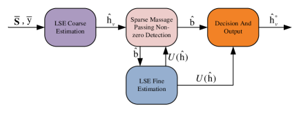
Figure 1: The processing for proposed LSE-SMP algorithm, which consists of three phases: Coarse Estimation, Sparse Message Passing Detection, and Fine Estimation.

fig:env

The fourier transformation $\mathbf{W}_{t}$ and $\mathbf{W}_{r}$ can be seen as a mapping from the antenna domain onto an angular domain and the entries of the matrix $\mathbf{H}_{v}$ can be interpreted as the channel gains between $N_{t}$ transmit and the $N_{r}$ receive beams. In this paper, we assume that the array response vectors are along the directions defined in the DFT matrices. This means that $\mathbf{H}_{v}$ is perfectly sparse, i.e., has exactly $L$ non-zero entries.

Assuming the channel is time-invariant in the blocks ${t\in\{1,...,T\}}$. Then, $\mathbf{Y}\triangleq[\mathbf{y}_{1},...,\mathbf{y}_{T}]$, $\mathbf{S}\triangleq[\mathbf{\mathbf{s}}_{1},...,\mathbf{s}_{T}]$ , and $\mathbf{N}\triangleq[\mathbf{\mathbf{n}}_{1},...,\mathbf{n}_{T}]$. We rewritten the channel model as:

$$\begin{split}\mathbf{Y}=\mathbf{W}_{r}\mathbf{H}_{v}\mathbf{W}_{t}^{H}\mathbf{S}+\mathbf{N}\end{split}$$ (9)

where $\mathbf{Y}\in\mathbb{C}^{N_{r}\times T}$, $\mathbf{S}\in\mathbb{C}^{N_{t}\times T}$, and $\mathbf{N}\in\mathbb{C}^{N_{r}\times T}$. We define $\mathbf{X}\triangleq\mathbf{W}_{t}^{H}\mathbf{S}$. Then, we recast the (9) as:

$$\begin{split}\mathbf{Y}=\mathbf{\mathbf{W}}_{r}\mathbf{H}_{v}\mathbf{X}+\bm{\mathbf{N}}\end{split}$$ (10)

Then, we can factorize the (10) [10] as:

$$\begin{split}vec(\mathbf{Y})&=vec(\mathbf{W}_{r}\mathbf{H}_{v}\mathbf{X}+\mathbf{N})\\ &\stackrel{{\scriptstyle(a)}}{{=}}(\mathbf{X}^{T}\otimes\mathbf{W}_{r})vec(\mathbf{H}_{v})+vec(\mathbf{N})\end{split}$$ (11)

where (a) follows from the equality $vec(\mathbf{ABC})=(\mathbf{C^{T}}\otimes\mathbf{A})vec(\mathbf{B})$. By defining the $\mathbf{\bar{S}}\triangleq\mathbf{X}^{T}\otimes\mathbf{W}_{r}$, we simply the (11) in a compact fashion.

$$\begin{split}\mathbf{\bar{y}}=\mathbf{\bar{S}}\mathbf{h}_{v}+\mathbf{\bar{n}}\end{split}$$ (12)

where $\mathbf{\bar{y}}\in\mathbb{C}^{N_{r}T\times 1}$, $\mathbf{\bar{S}}\in\mathbb{C}^{N_{r}T\times N_{t}N_{r}}$, $\mathbf{h}_{v}\in\mathbb{C}^{N_{t}N_{r}\times 1}$ and $\mathbf{\bar{n}}\in\mathbb{C}^{N_{r}T\times 1}$. The mmWave channel estimation problem is simplified to estimate virtual channel vector $\mathbf{h}_{v}$ by giving the equivalent training matrix $\mathbf{\bar{S}}$ and the observed signal $\mathbf{\bar{y}}$.

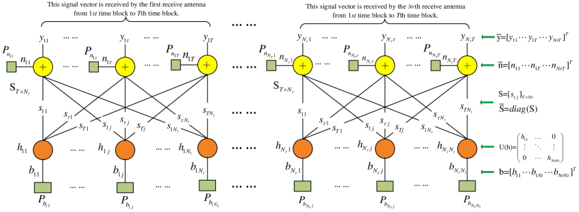
Figure 2: Factor Graph Representation for Proposed Sparse Message Passing (SMP) Detection Algorithm

III SPARSE CHANNEL ESTIMATION

In this section, we present a novel channel estimation algorithm based on the LSE and SMP algorithm, which is named LSE-SMP, and it consists of three phases: Coarse Estimation, Message Passing Detection, and Fine Estimation. This algorithm is shown in the Fig. 1. Since there is no priori knowledge of $\mathbf{h}_{v}$, we initially adopt LSE method to obtain its coarse estimation. Then, we consider the estimation of non-zero positions in the channel vector $\mathbf{h}_{v}$ as a detection problem, and propose a SMP algorithm to find these non-zero positions. Again, we apply LSE method by leveraging the estimated non-zero positions to obtain the fine estimation. The second step and third step will repeat until we obtain the steady estimation.

III-A LSE Coarse Estimation

To find Coarse Estimation $\mathbf{\hat{h}}_{v}$ based on the observed vector $\mathbf{\bar{y}}$, with a Mean Square Error (MSE), we can solve the following Least Square (LS) problem:

$$\begin{split}\mathbf{\hat{h}}_{v}&=arg\min_{\mathbf{h}_{v}}\|\mathbf{\bar{y}}-\mathbf{\bar{S}}\mathbf{h}_{v}\|^{2}_{2}\\ &=[\mathbf{\bar{S}}^{T}\mathbf{\bar{S}}]^{-1}\mathbf{\bar{S}}^{T}\mathbf{\bar{y}}\end{split}$$ (13)

It is noted that it is optimal estimator in the sense of MSE when the estimator does not have any prior knowledge about neither the sparsity structure of $\mathbf{h}_{v}$ (i.e. the location of non-zero entries), nor its degree of sparsity (i.e. $L$ ).

III-B Sparse Message Passing Algorithm

After we get the Coarse Estimation of $\mathbf{h}_{v}$, we propose a fast iterative algorithm to find the positions of non-zero entries. This algorithm is named Sparse Message Passing since it can take full advantage of channel sparsity and message passing.

III-B1 Factor Graph Representation of mmWave Channel

In order to get better understanding of our proposed algorithm, we show factor graph representation of channel vector $\mathbf{h}_{v}$ in the following. Firstly, we decompose the $\mathbf{h}_{v}$ into a diagonal coefficient matrix $\mathbf{U}(h_{ij})(i\in[{0,...,N_{r}}],j\in[{0,...,N_{t}}])$ and a column array b. The column array $\textbf{b}=[b_{ij}]_{N_{r}N_{t}\times 1}$ is called position vector, and it represents the positions of non-zero in virtual channel vector $\mathbf{h}_{v}$. The $b_{ij}\in\{1,0\}$ can be seen as a Bernoulli distribution. Then, the $\mathbf{h}_{v}$ can be recast as:

$$\begin{split}\mathbf{h}_{v}=\underbrace{\left[\begin{array}[]{ccccc}h_{11}&&&&0\\ &\ddots&&\\ &&h_{1N_{t}}&\\ &&&\ddots&\\ 0&&&&h_{N_{r}N_{t}}\\ \end{array}\right]}_{=\mathbf{U(h)}}\underbrace{\left[\begin{array}[]{cccc}b_{11}\\ \vdots\\ b_{1N_{t}}\\ \vdots\\ b_{N_{r}N_{t}}\end{array}\right]}_{=\mathbf{b}}\end{split}$$ (14)

The equivalent training matrix $\mathbf{\bar{S}}$ can be expressed as the following block diagonal matrix by designing $\mathbf{X}$ and $\mathbf{W}_{r}$.

$$\begin{split}\mathbf{\bar{S}}=diag(\mathbf{S})\end{split}$$ (15)

where $\mathbf{\bar{S}}\in\mathbb{C}^{N_{r}T\times NrN_{t}}$, and $\mathbf{S}$ can be seen as a matrix of transmitted training sequences, which will be received by $i$th $(i\in{[1,...,N_{r}]})$ receive antenna from 1 to $T$th time block. It can be written as:

$$\begin{split}\mathbf{S}=[s_{\tau j}]_{T\times N_{t}}\end{split}$$ (16)

where $s_{\tau j}$ represents the transmitted training sequences by $j$th $(j\in{[1,...,N_{t}]})$ transmit antenna in the $\tau$th $(\tau\in{[1,...,T]})$ time block. Then, we rewrite (12) as:

$$\begin{split}\!\!\!\!\!\!\underbrace{\left[\begin{array}[]{ccccc}y_{11}&\ldots&y_{1T}&\ldots&y_{N_{r}T}\end{array}\right]^{T}}_{\mathbf{\bar{y}}}&=\mathbf{\bar{S}}\mathbf{h}_{v}+\mathbf{\bar{n}}\\ &=\mathbf{\bar{S}}\mathbf{U(h)b}+\mathbf{\bar{n}}\end{split}$$ (17)

According to the factor graph analysis rule, we plot a factor graph to represent above equations, and it is shown in the Fig. 2. The nodes ($n_{11},...,n_{N_{r}T}$) and ($h_{11},...,h_{N_{r}N_{t}}$) are named the sum and variable nodes respectively.

Our proposed SMP algorithm is considered for estimating positions of non-zero. It is similar to the belief propagation decoding process of low density parity check code, in which the output message called extrinsic information on each edge is calculated by the messages on the other edges that are connected with the same node [14].

III-B2 Message Update at Sum Nodes of SMP

To analysis a sum node that is shown in the Fig. 3, we can know the received signal at the $\tau$th time block by the $i$th receive antenna, and it can be expressed as:

$$\vspace{-1mm}\begin{split}y_{i\tau}=\sum_{j=1}^{N_{t}}s_{\tau j}h_{ij}b_{ij}+n_{i\tau}\end{split}$$ (18)

From assumption of channel model in the above section, we know that there are $L$ non-zero in the vector of $\mathbf{b}$. Assuming that $b_{ij}$ is independent and identically distributed (i.i.d.). Then, we can know the initial probability of the Bernoulli distribution, which can be denoted as:

$$\left\{\begin{array}[]{l}p_{0}(b_{ij}=1)=\frac{L}{N_{r}N_{t}},\\ p_{0}(b_{ij}=0)=1-\frac{L}{N_{r}N_{t}}.\end{array}\right.\quad$$ (19)

According to the law of large numbers, when $N_{t}$ goes very large, we can know the term $\sum_{j=1}^{N_{t}}s_{\tau j}h_{ij}b_{ij}$ can be approximated as Gaussian distribution [15]. When we compute the probability of $p(b_{ij}=1)$ from $i\tau$ sum node to $ij$ variable node, we consider the messages from other variable nodes to sum node $i\tau$ as noise. This can be expressed as:

$$\begin{split}\!\!\!\!y_{i\tau}\!\!=\!\!\underbrace{s_{\tau j}h_{ij}p(b_{ij}=1)}_{desired}+\underbrace{\sum_{m\neq j}^{N_{t}}s_{\tau m}h_{im}p(b_{im}=1)+n_{i\tau}}_{{interference}}\end{split}$$ (20)

Furthermore, we can compute its mean value and variance. The message update at the sum nodes is given by:

$$\left\{\begin{array}[]{l}e^{s}_{i\tau\rightarrow ij}(k)=\sum\limits_{m\neq j}s_{\tau m}\hat{h}_{im}p^{v}_{im\rightarrow i\tau}(k-1),\\ v^{s}_{i\tau\rightarrow ij}(k)={\sum\limits_{m\neq j}}s^{2}_{\tau m}p^{v}_{im\rightarrow i\tau}(k-1)\\ \times(v_{h_{im}}+\hat{h}_{im}^{2}(1-p^{v}_{im\rightarrow i\tau}(k-1)))+\sigma^{2}_{n}.\end{array}\right.$$ (21)

where $j,m\in\{1,2,...,N_{t}\}$, $\sigma^{2}_{n}$ is the variance of the Gaussian noise. In addtion, $p^{v}_{im\rightarrow i\tau}(k-1)$ denotes the probability message of passing from the $im$ variable node to $i\tau$ sum node at $(k-1)$th iteration [16]. Similarly, $e^{s}_{i\tau\rightarrow ij}(k)$ and $v^{s}_{i\tau\rightarrow ij}(k)$ denote the mean and variance of $s_{\tau j}h_{ij}$ passing from the $i\tau$ sum node to $ij$ variable node at $k$th iteration respectively. $\hat{h}_{im}$ and $v_{h_{im}}$ denote the mean and variance of $h_{im}$ that are estimated in the fine phase.

Once we get the mean and variance from the $i\tau$ sum node to $ij$ variable node, we can compute its statistical probability according to the $s_{\tau j}h_{ij}p(b_{ij}=1)\sim\mathcal{N}(e^{s}_{i\tau\rightarrow ij}(k),v^{s}_{i\tau\rightarrow ij}(k))$. Firstly, we define the Gaussian probability density function as:

$$f(x|\mu,\sigma)=\frac{1}{\sqrt{2\pi}\sigma}e^{-\frac{(x-\mu)^{2}}{2\sigma^{2}}}$$ (22)

Then, we can give the probability from the $i\tau$ sum node to $ij$ variable node as follow:

$$\!\!\!p^{s}_{i\tau\rightarrow ij}(k)\!\!=\!\!\frac{1}{1+\frac{f(y_{i\tau}|e^{s}_{i\tau\rightarrow ij}(k),v^{s}_{i\tau\rightarrow ij}(k))}{f(y_{i\tau}|e^{s}_{i\tau\rightarrow ij}(k)+s_{\tau j}\hat{h}_{ij},v^{s}_{i\tau\rightarrow ij}(k)+s^{2}_{\tau j}v_{h_{ij}})}}$$ (23)

III-B3 Message Update at Variable Nodes of SMP

In terms of the message update at variable nodes, we consider variable nodes as a broadcast process [14] and the message update at these nodes is given by:

$$p^{v}_{ij\rightarrow i\tau}(k)=\frac{1}{1+\frac{\prod_{t\neq\tau}(1-p^{s}_{it\rightarrow ij}(k-1))\cdot p_{0}(b_{ij}=0)}{\prod_{t\neq\tau}p^{s}_{it\rightarrow ij}(k-1)\cdot p_{0}(b_{ij}=1)}}$$ (24)

where $t,\tau\in\{1,2,...,T\}$, and, $p^{s}_{it\rightarrow ij}(k-1)$ denotes the probability message passing from the $it$ sum node to $ij$ variable node at $(k-1)$th iterations.

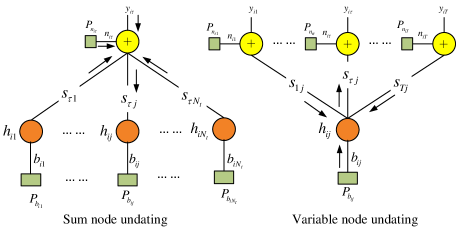
Figure 3: Message update at sum nodes and variable nodes. The output message called extrinsic information on each edge is calculated by the messages on the other edges that are connected with the same node. For the Gaussian-Bernoulli sparse signals, the messages passing on each edge are the mean and variance of a Gaussian distribution, and the non-zero probability of a Bernoulli distribution.

III-C LSE Fine Estimation

Once the positions of the non-zero have been detected, the next step is to estimate the value of coefficient matrix $\mathbf{U}(h)$. For the problem, we propose a novel strategy based on LSE method. This strategy is to swap the position of $h_{ij}$ and $b_{ij}$ in the (17), so that we can get an accurate estimation by leveraging sparsity of b. Rewriting the (17) as:

$$\mathbf{\bar{y}}=\mathbf{\bar{S}}\mathbf{U(b)h}+\mathbf{\bar{n}}$$ (25)

where $\mathbf{h}\in\mathbb{C}^{N_{t}N_{r}\times 1}$. Similar with Coarse Estimation, the estimation of $\mathbf{h}$ can be found by solving the following LS problem:

$$\mathbf{\hat{h}}=arg\min_{\tilde{\mathbf{h}}}\{\|\mathbf{\bar{y}}-\mathbf{\bar{S}}\mathbf{U(\hat{b}})\mathbf{\tilde{h}}\|^{2}_{2}\}$$ (26)

where $\mathbf{\hat{b}}$ is the vector obtained by SMP algorithm. Calculating the gradient of the above expression with respect to $\tilde{\mathbf{h}}$ and setting it to zero, we get the following estimator for $\tilde{\mathbf{h}}$ :

$$\left\{\begin{array}[]{l}\mathbf{\hat{h}}(k)=\mathbf{\hat{Q}}^{\dagger}(k-1)(\mathbf{\bar{S}}\mathbf{U}(\mathbf{\hat{b}(k-1)}))^{T}\mathbf{\bar{y}}\\ \mathbf{V}_{h}(k)=\sigma^{2}_{n}(\mathbf{\bar{S}}\mathbf{U}(\mathbf{\hat{b}}(k-1)))^{T}\mathbf{\bar{S}}\mathbf{U}(\mathbf{\hat{b}}(k-1))\end{array}\right.\quad$$ (27)

where $\mathbf{\hat{Q}}(k-1)=\mathbf{U}(\mathbf{\hat{b}}(k-1))\mathbf{\bar{S}}^{T}\mathbf{\bar{S}}\mathbf{U}(\mathbf{\hat{b}}(k-1))$, $\mathbf{V}_{h}=[v_{h_{im}}]_{N_{r}N_{t}\times 1},i\in\{1,2,...,N_{r}\}$ and $m\in\{1,2,...,N_{t}\}$. $\mathbf{\hat{h}(k)}$ and $\mathbf{V}_{h}$ denotes the estimated value and variance of $\mathbf{h}$ at $k$th iteration. After we obtain $\mathbf{\hat{h}}(k)$, this value will replace the $\mathbf{\hat{h}}(k-1)$ for calculating $\mathbf{\hat{b}}(k)$ by applying SMP algorithm.

III-D Decision and Output of LSE-SMP

When the MSE of the LSE-SMP meets the requirement or the number of iterations reaches the limit, we output:

$$\vspace{-0mm}\hat{b}_{ij}=\frac{1}{1+\frac{\prod_{t=1}^{T}(1-p^{s}_{it\rightarrow tj}(k))\cdot p_{0}(b_{ij}=0)}{\prod_{t=1}^{T}p^{s}_{it\rightarrow tj}(k)\cdot p_{0}(b_{ij}=1)}}$$ (28)

and

$$\left\{\begin{array}[]{l}\hat{\mathbf{h}}=\mathbf{\hat{Q}}^{\dagger}(\mathbf{\bar{S}}\mathbf{U}(\mathbf{\hat{b}}))^{T}\mathbf{\bar{y}},\\ \mathbf{\hat{h}}_{v}^{*}=\mathbf{U}(\mathbf{\hat{h}})\mathbf{\hat{b}}.\end{array}\right.\quad$$ (29)

where $\mathbf{\hat{h}}_{v}^{*}$ is the finally outputted channel estimation vector. It should be pointed out that the decision is made based on full information coming from all the sum nodes.

IV ANALYSIS OF CRAMER RAO BOUND

In this section, we give the analysis of Cramer-Rao bound and show that our proposed LSE-SMP algorithm is unbiased. We begin with conventional LSE that is applied for a deterministic and non-sparse channel vector $\mathbf{h}_{v}$. From [17] and recalling the signal model in (13), the CRLB is yielded as:

$$\mathbf{CRLB_{LSE}}\geq\sigma^{2}_{n}(\mathbf{\bar{S}}^{T}\mathbf{\bar{S}})^{-1}$$ (30)

Note that LSE is the Minimum Variance Unbiased Estimator (MVUE), if $\mathbf{h}_{v}$ is deterministic and non-sparse.

Compared with the non-sparse case, the sparse situation is slightly more complicated. As we are interested in the lower bound for the estimation accuracy, we assume perfect knowledge of the non-zero positions, i.e. $\mathbf{U}(\mathbf{\hat{b}})=\mathbf{b}$. Then, the next step is to verify the estimator is unbiased. Recalling the signal model in (25) and from the definition of unbiased estimator, we get:

$$\!\!E(\mathbf{\hat{h}}_{v}) \!=\!\!E(((\mathbf{\bar{S}}\mathbf{U}(\mathbf{b}))^{T}\mathbf{\bar{S}}\mathbf{U}(\mathbf{b}))^{\dagger}(\mathbf{\bar{S}}\mathbf{U}(\mathbf{b}))^{T}\mathbf{\bar{y}})$$

$$\!\!=\!\!E(((\mathbf{\bar{S}}\mathbf{U}(\mathbf{b}))^{T}\mathbf{\bar{S}}\mathbf{U}(\mathbf{b}))^{\dagger}(\mathbf{\bar{S}}\mathbf{U}(\mathbf{b}))^{T}(\mathbf{\bar{S}}\mathbf{U}(\mathbf{b})\mathbf{h}+\mathbf{\bar{n}}))$$

$$\!\!=\!\!\mathbf{U}(\mathbf{b})\mathbf{h}=\mathbf{h}_{v}$$ (31)

So, it is a unbiased estimator. The next step is to compute its CRLB. As previously mentioned, the channel $\mathbf{h}_{v}$ is a deterministic vector, we can get:

$$\mathbf{\bar{y}}\sim p(\mathbf{\bar{y}};\mathbf{h}_{v})=\mathcal{N}(\mathbf{\bar{S}}\mathbf{h}_{v},\sigma^{2}_{n}\mathbf{I})$$ (32)

Then, we can compute the $\frac{\partial ln\,p(\mathbf{\bar{y}};\mathbf{h}_{v})}{\partial\mathbf{h}_{v}}$,

$$\!\!\!\!\frac{\partial ln\,p(\mathbf{\bar{y}};\mathbf{h}_{v})}{\partial\mathbf{h}_{v}}\!\!=\!\!\frac{1}{\sigma_{n}^{2}}[(\mathbf{\bar{S}}\mathbf{U}(\mathbf{b}))^{T}\mathbf{\bar{y}}-(\mathbf{\bar{S}}\mathbf{U}(\mathbf{b}))^{T}\mathbf{\bar{S}}\mathbf{U}(\mathbf{b})\mathbf{h}_{v}]$$ (33)

Then, we obtain the following expression for the Fisher Information Matrix (FIM):

$$I(\mathbf{h}_{v})=-E(\frac{\partial^{2}ln\,p(\mathbf{\bar{y}};\mathbf{h}_{v})}{\partial\mathbf{h}^{2}_{v}})\\ =\frac{1}{\sigma_{n}^{2}}{{(\mathbf{\mathbf{\bar{S}}}\mathbf{U}(\mathbf{b}))^{T}\mathbf{\bar{S}}}\mathbf{U}(\mathbf{b})}$$ (34)

We note that $\mathbf{\bar{S}}\mathbf{U}(\mathbf{b})$ has the rank no larger than $L$ due to the multiplication of $\mathbf{\bar{S}}$ by $\mathbf{U}(\mathbf{b})$. The matrices $\mathbf{\bar{S}}\mathbf{U}(\mathbf{b})$ and $(\mathbf{\bar{S}}\mathbf{U}(\mathbf{b}))^{T}$ have some all zero columns (and rows), so it is singular. For this type singular matrix, it need to meet the following constraint [18], otherwise our proposed estimator (29) has infinite variance that renders the CRLB useless. Before we analyze this constraint, we firstly compute the following key identity:

$$\begin{split}\mathbf{G}&=((\mathbf{\bar{S}}\mathbf{U}(\mathbf{b}))^{T}\mathbf{\bar{S}}\mathbf{U}(\mathbf{b}))^{\dagger}(\mathbf{\bar{S}}\mathbf{U}(\mathbf{b}))^{T}\mathbf{\bar{S}}\mathbf{U}(\mathbf{b})\\ &=diag(\mathbf{b})\neq\mathbf{I}_{N_{r}N_{t}}\end{split}$$ (35)

This constraint is given by:

$$\mathbf{G}=\mathbf{G}I(\mathbf{h}_{v})I(\mathbf{h}_{v})^{\dagger}$$ (36)

plugging the (34) and (35) into (36), we obtain $\mathbf{G}=\mathbf{G}I(\mathbf{h}_{v})I(\mathbf{h}_{v})^{\dagger}=\mathbf{U(b)U(b)}$ that holds. This means that the variance of our proposed estimator is finite. Since the FIM $I(\mathbf{h}_{v})$ in (34) is singular, the expression for the CRLB can be computed following [18] which yields:

$$\begin{split}\mathbf{CRLB_{LSE-SMP}}&\geq\mathbf{G}I(\mathbf{h}_{v})^{\dagger}\mathbf{G}^{T}\\ &=\sigma^{2}_{n}(\mathbf{\bar{S}}\mathbf{U}(\mathbf{b}))^{T}\mathbf{\bar{S}}\mathbf{U}(\mathbf{b})\end{split}$$ (37)

V NUMERICAL RESULTS

In this section, we investigate the performance of the our proposed algorithm using Monte-Carlo simulations, comparing with the LASSO sparse estimator and CRLB. We demonstrate that ours proposed LSE-SMP algorithm provides significant performance gains over existing techniques. In particular, we show that our proposed algorithm specialize in the mmWave channel estimation. Furthermore, we conduct numerical studies to investigate the impact of channel sparse ratios and iterations.

V-A Setup

For our numerical study, we considered the channel estimation problem in a $32\times 64$ mmWave MIMO system. The value and positions of non-zero elements in original channel vector $\mathbf{h}_{v}$ were both generated by random way with a distribution following $\mathcal{N}(0,\sqrt{10})$. Throughout, we considered SNR $\triangleq E\{\|\mathbf{\bar{S}}\|^{2}_{F}/\|\mathbf{\bar{n}}\|^{2}_{F}\}$ in the interval [-10, 40dB]; sparsity ratio was calculated by $\eta=L/(N_{r}\times N_{t})$; and the performance metric was the Normalized Mean Square Error (NMSE), given by $E\{\frac{\|\mathbf{\hat{h}}_{v}^{*}-\mathbf{h}_{v}\|^{2}_{F}}{\|\mathbf{h}_{v}\|^{2}_{F}}\}$.

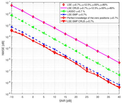
Figure 4: Average NMSE performance comparison of proposed LSE-SMP, conventional LSE, and LASSO channel estimates versus SNR for the sparsity ratio at $\eta=0.7\%$ with the 5 iterations. It also shows CRLB of LSE and proposed LSE-SMP.

V-B Performance Comparison

Fig. 4 shows the average channel-estimation NMSE of our proposed LSE-SMP algorithm and LASSO under the sparse ratio at $0.7\%$. Additionally, we also compute the CRLB for the classical LSE and our proposed LSE-SMP estimator. Our proposed LSE-SMP estimator obtains the better NMSE performance than that of LASSO and LSE. As expected, the CRLB for our proposed LSE-SMP is the lowest, and this result is also consistent with that of classical LSE estimator with perfect knowledge of the non-zero positions. It is also seen from the Fig.4 that the gap between LSE-SMP and LSE-SMP CRLB is much smaller, about $1.5dB$. This is partly due to the errors in the detection of the non-zero positions in sparse message passing phase and partly to the fact that all our detection strategies rely on a coarse (and noisy) initial estimate of the channel.

V-C Effect of Sparsity Ratio

For further investigating the effect of sparsity ratio to our proposed algorithm, we fixed the iteration times $=5$, and changed the sparsity ratio $\eta$ from $0.7\%$ to $80\%$. Note that different sparsity ratios $\eta$ will leads to different LSE-SMP CRLBs. Simulations show that the NMSE performance of the LSE-SMP is very close to its CRLB in the each of sparsity ratios. In the Fig. 5, we just give the LSE-SMP CRLB at the sparse ratio $\eta=0.7\%$. We can see that the NMSE performance of LSE is consistent LSE CRLB, and it is also the upper bound of LSE-SMP. These verify the analysis of LSE-SMP in the IV section. It means that the NMSE performance of LSE-SMP will be better with decreasing of sparse ratios as shown in the Fig. 5, essentially because LSE-SMP is able to exploit the sparsity of the channel. To be specific, The NMSE performance of LSE keep unchange under different sparsity ratios. On the other hand, the NMSE performance of LSE-SMP will increase with the decreasing of sparsity ratios. This means that LSE-SMP scheme will perform better especially when channel is very sparse.

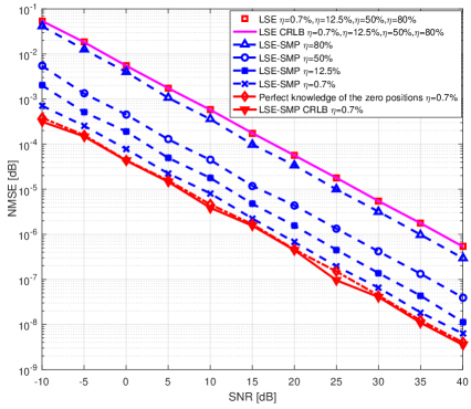
Figure 5: Average NMSE performance comparison of LSE-SMP, LSE and their CRLB channel estimates versus SNR for different sparsity ratios $\eta\in\{0.7\%,12.5\%,50\%,80\%\}$ with the iteration $=5$. It can be seen that LSE CRLB is the upper bound and LSE-SMP CRLB is the low bound of our proposed LSE-SMP.

V-D Effect of Iterations

Fig. 6 shows the average channel-estimation NMSE performance for LSE-SMP algorithm under several turbo iterations with sparsity ratio $\eta=3.1\%$. The result shows that after the second turbo iteration, the NMSE performance of LSE-SMP performs a significant improvement. Additionally, we also find that the gap of the NMSE performance between the adjacent iterations for LSE-SMP algorithm will be decreasing with increasing of iterations. After fourth turbo iteration, the NMSE performance have no significant improvement and it is very close to our analyzed LSE-SMP CRLB. This demonstrates that the convergence speed of the LSE-SMP algorithm is fast.

VI CONCLUSION

In this paper, a novel channel estimation algorithm for mmWave MIMO systems was proposed, which can take full advantage of the inherent sparseness of mmWave channel. This algorithm leverages the virtues of the SMP and LSE algorithm. The CRLB for the proposed LSE-SMP algorithm was analyzed. Simulation experiments verified that our proposed algorithm had much better performance than the existing sparse estimators, especially when channel is very sparse. Furthermore, it was also shown that the proposed algorithm needs only several turbo iterations to achieve CRLB. In spite of this, it still has the high complexity due to the computation of inverse matrixes in coarse and fine estimation phases. In the following, we plan to develop an approach to replace the LSE coarse and fine estimation without loss of global performance of the algorithm. Another limitation in our paper is the assumption that virtual channel vector $\mathbf{h}_{v}$ has exactly $L$ non-zero entries. In the future work, we will also consider to relax the assumption.

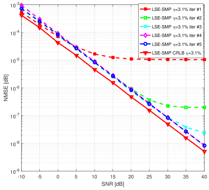
Figure 6: Average NMSE performance comparison of LSE-SMP and its CRLB channel estimates versus SNR for different turbo iterations with the sparsity ratio $\eta=3.1\%$. After the fourth iteration, the NMSE performance of LSE-SMP is converging to its CRLB.

References

- [1] T. Rappaport, S. Sun, R. Mayzus, H. Zhao, Y. Azar, K. Wang, G. Wong, J. Schulz, M. Samimi, and F. Gutierrez, “Millimeter wave mobile communications for 5G cellular: It will work” IEEE Access, vol. 1, pp. 335 C349, 2013.
- [2] R. W. Heath Jr., N. G. Prelcic, S. Rangan, W. Roh, and A. Sayeed, “An Overview of Signal Processing Techniques for Millimeter Wave MIMO Systems,” to appear in IEEE Journal of Selected Topics in Signal Processing, Apr. 2016.
- [3] T. S. Rappaport, G. R. MacCartney, Jr., M. K. Samimi, and S. Sun,“Wideband millimeter-wave propagation measurements and channel models for future wireless communication system design” IEEE Transactions on Communications, vol. 63, no. 9, pp. 3029-3056, Sept. 2015.
- [4] P. Schniter and A. M. Sayeed, “A Sparseness-Preserving Virtual MIMO Channel Model,” in Proc. Conf. on Information Sciences and Systems, (Princeton, NJ), pp. 36-41, Mar. 2004.
- [5] Y. Zhu, D. Guo and M. L. Honig, “A message-passing approach for joint channel estimation, interference mitigation, and decoding,” IEEE Transactions on Wireless Communications, vol. 8, no. 12, pp. 6008-6018, Dec. 2009.
- [6] S. Wu, L. L. Kuang, Z. Y. Ni, D. Huang, Q. H. Guo and J. H. Lu, “Message-Passing Receiver for Joint Channel Estimation and Decoding in 3D Massive MIMO-OFDM Systems” submitted to IEEE Transactions on Wireless Communications,Jan. 2016.
- [7] R. Tibshirani,“Regression shrinkage and selection via the lasso” J. Roy. Statist. Soc. B, vol. 58, no. 1, pp. 267 288, 1996.
- [8] C. Carbonelli, S. Vedantam and U. Mitra, “Sparse Channel Estimation with Zero Tap Detection,” IEEE Transactions on Wireless Communications, vol. 6, no. 5, pp. 1743-1763, May 2007.
- [9] R. Niazadeh, M. Babaie-Zadeh, and C. Jutten, “An alternating minimization method for sparse channel estimation,” in Proc. 9th Int. Conf. Latent Variable Anal. Signal Seperation, 2010, pp. 319 C327.
- [10] A. Alkhateeb, O. El Ayach, G. Leus and R. W. Heath, ”Channel Estimation and Hybrid Precoding for Millimeter Wave Cellular Systems,” in IEEE Journal of Selected Topics in Signal Processing, vol. 8, no. 5, pp. 831-846, Oct. 2014.
- [11] A. M. Sayeed, “Deconstructing multi-antenna fading channels,” IEEE Trans. on Signal Processing, pp. 2563 C2579, Oct. 2002.
- [12] J. Mo, P. Schniter, N. Gonzalez-Prelcic, and R. W. Heath, Jr., “Channel estimation in millimeter wave MIMO systems with one-bit quantization” in Proc. Asilomar Conf. on Signals, Systems and Computers, Nov. 2014.
- [13] P. Schniter and A. Sayeed, “Channel Estimation and Precoder Design for Millimeter-Wave Communications: The Sparse Way,” in Proc. Asilomar Conf. on Signals, Systems, and Computers, Nov. 2014
- [14] L. Liu, Y. Li, Y. Su, and Y. Sun, “Quantize-and-Forward Strategy for Interleave-Division Multiple-Access Relay Channel,” IEEE Transactions on Vehicular Technology 65(3): 1808-1814, 2016.
- [15] L. Liu, C. Yuen, Y. L. Guan, Y. Li and Y. P. Su, “Convergence Analysis and Assurance Gaussian Message Passing Iterative Detection for Massive MU-MIMO Systems,” IEEE Transactions on Wireless Communications, to be published.
- [16] L. Liu, C. Yuen, Y. L. Guan, Y. Li and C. W. Huang, “Gaussian Message Passing Iterative Detection for MIMO-NOMA Systems With Massive Users,” IEEE Global Communications Conference (GlobeCom2016), Washington, DC USA, 2016
- [17] A.Van den Bos, Parameter estimation for scientists and engineers. John Wiley and Sons, 2007.
- [18] P. Stoica and T. L. Marzetta, “Parameter estimation problems with singular information matrices,” IEEE Trans. Signal Processing, vol. 49, no. 1, pp. 87-89, Jan. 2001.