A tool for stability and power sharing analysis of a generalized class of droop controllers for high-voltage direct-current transmission systems

Abstract

The problem of primary control of high-voltage direct current transmission systems is addressed in this paper, which contains four main contributions. First, to propose a new nonlinear, more realistic, model for the system suitable for primary control design, which takes into account nonlinearities introduced by conventional inner controllers. Second, to determine necessary conditions—dependent on some free controller tuning parameters—for the existence of equilibria. Third, to formulate additional (necessary) conditions for these equilibria to satisfy the power sharing constraints. Fourth, to establish conditions for stability of a given equilibrium point. The usefulness of the theoretical results is illustrated via numerical calculations on a four-terminal example.

I INTRODUCTION

For its correct operation, high-voltage direct current (hvdc) transmission systems—like all electrical power systems—must satisfy a large set of different regulation objectives that are, typically, associated to the multiple time–-scale behavior of the system. One way to deal with this issue, that prevails in practice, is the use of hierarchical control architectures [1, 2, 3]. Usually, at the top of this hierarchy, a centralized controller called tertiary control—based on power flow optimization algorithms (OPFs)—is in charge of providing the inner controllers with the operating point to which the system has to be driven, according to technical and economical constraints [1]. If the tertiary control had exact knowledge of such constraints and of the desired operating points of all terminals, then it would be able to formulate a nominal optimization problem and the lower level (also called inner-loop) controllers could operate under nominal conditions. However, such exact knowledge of all system parameters is impossible in practice, due to uncertainties and lack of information. Hence, the operating points generated by the tertiary controller may, in general, induce unsuitable perturbed conditions. To cope with this problem further control layers, termed primary and secondary control, are introduced. These take action—whenever a perturbation occurs—by promptly adjusting the references provided by the tertiary control in order to preserve properties that are essential for the correct and safe operation of the system. The present paper focuses on the primary control layer. Irrespectively of the perturbation and in addition to ensuring stability, primary control has the task of preserving two fundamental criteria: a prespecified power distribution (the so-called power sharing) and keeping the terminal voltages near the nominal value [4]. Both objectives are usually achieved by an appropriate control of the dc voltage of one or more terminals at their point of interconnection with the hvdc network [5, 6, 2].
Clearly, a sine qua non requirement for the fulfillment of these objectives is the existence of a stable equilibrium point for the perturbed system. The ever increasing use of power electronic devices in modern electrical networks, in particular the presence of constant power devices (CPDs), induces a highly nonlinear behavior in the system—rendering the analysis of existence and stability of equilibria very complicated. Since linear, inherently stable, models, are usually employed for the description of primary control of dc grids [6, 3, 7], little attention has been paid to the issues of stability and existence of equilibria. This fundamental aspect of the problem has only recently attracted the attention of power systems researchers [8, 9, 10] who, similarly to the present work, invoke tools of nonlinear dynamic systems analysis, to deal with the intricacies of the actual nonlinear behavior.

The main contributions and the organization of the paper are as follows. Section II is dedicated to the formulation—under some reasonable assumptions—of a reduced, nonlinear model of an hvdc transmission system in closed-loop with standard inner-loop controllers. In Section III a further model simplification, which holds for a general class of dc systems with short lines configurations, is presented. A first implication is that both obtained models, which are nonlinear, may in general have no equilibria. Then, we consider a generalized class of primary controllers, that includes the special case of the ubiquitous voltage droop control, and establish necessary conditions on the control parameters for the existence of an equilibrium point. This is done in Section IV. An extension of this result to the problem of existence of equilibria that verify the power sharing property is carried out in Section V. A last contribution is provided in Section VI, with a (local) stability analysis of a known equilibrium point, based on Lyapunov’s first method. The usefulness of the theoretical results is illustrated with a numerical example in Section VII. We wrap-up the paper by drawing some conclusions and providing guidelines for future investigation.

Notation. For a set $\mathcal{N}=\{l,k,\dots,n\}$ of, possibly unordered, elements, we denote with $i\sim\mathcal{N}$ the elements $i=l,k,\dots,n$. All vectors are column vectors. Given positive integers $n$, $m$, the symbol $0_{n}\in\mathbb{R}^{n}$ denotes the vector of all zeros, $0_{n\times m}$ the $n\times m$ column matrix of all zeros, $\mathsf{1}_{n}\in\mathbb{R}^{n}$ the vector with all ones and $\mathbb{I}_{n}$ the $n\times n$ identity matrix. When clear from the context dimensions are omitted and vectors and matrices introduced above are simply denoted by the symbols $0$, $\mathsf{1}$ or $\mathbb{I}$. For a given matrix $A$, the $i$-th colum is denoted by $A_{i}$. Furthermore, $\mbox{diag}\{a_{i}\}$ is a diagonal matrix with entries $a_{i}\in\mathbb{R}$ and $\text{bdiag}\{A_{i}\}$ denotes a block diagonal matrix with matrix-entries $A_{i}$. $x:=\mbox{col}(x_{1},\dots,x_{n})\in\mathbb{R}^{n}$ denotes a vector with entries $x_{i}\in\mathbb{R}$. When clear from the context it is simply referred to as $x:=\mbox{col}(x_{i})$.

II NONLINEAR MODELING OF HVDC TRANSMISSION SYSTEMS

II-A A graph description

The main components of an hvdc transmission system are ac to dc power converters and dc transmission lines. The power converters connect ac subsystems—that are associated to renewable generating units or to ac grids—to an hvdc network. In [11] it has been shown that an hvdc transmission system can be represented by a directed graph without self-loops, where the power units—i.e. power converters and transmission lines—correspond to edges and the buses correspond to nodes. Hence, a first step towards the construction of a suitable model for primary control analysis and design is then the definition of an appropriate graph description of the system topology that takes into account the primary control action.

We consider an hvdc transmission system described by a graph $\mathcal{G}^{\uparrow}(\mathcal{N},\mathcal{E})$, where $\mathsf{n}=\mathsf{c}+1$ is the number of nodes, where the additional node is used to model the ground node, and $\mathsf{m}=\mathsf{c}+\mathsf{t}$ is the number of edges, with $\mathsf{c}$ and $\mathsf{t}$ denoting the number of converter and transmission units respectively. We implicitly assumed that transmission (interior) buses are eliminated via Kron reduction [12]. We further denote by $\mathsf{p}$ the number of converter units not equipped with primary control—termed PQ units hereafter—and by $\mathsf{v}$ the number of converter units equipped with primary control—that we call voltage-controlled units, with $\mathsf{c}=\mathsf{p}+\mathsf{v}.$ To facilitate reference to different units we find it convenient to partition the set of converter nodes (respectively converter edges) into two ordered subsets $\mathcal{N}_{P}$ and $\mathcal{N}_{V}$ (respectively $\mathcal{E}_{P}$ and $\mathcal{E}_{V}$) corresponding to $PQ$ and voltage-controlled nodes (respectively edges). The incidence matrix associated to the graph is given by:

$$\mathcal{B}=\begin{bmatrix}\mathbb{I}_{\mathsf{p}}&0&\mathcal{B}_{{P}}\\ 0&\mathbb{I}_{\mathsf{v}}&\mathcal{B}_{{V}}\\ -\mathsf{1}^{\top}_{\mathsf{p}}&-\mathsf{1}^{\top}_{\mathsf{v}}&0\end{bmatrix}\in\mathbb{R}^{\mathsf{n}\times\mathsf{m}},$$ (II.1)

where the submatrices $\mathcal{B}_{{P}}\in\mathbb{R}^{\mathsf{p}\times\mathsf{t}}$ and $\mathcal{B}_{{V}}\in\mathbb{R}^{\mathsf{v}\times\mathsf{t}}$ fully capture the topology of the hvdc network with respect to the different units.

II-B Converter units

For a characterization of the converter units we consider power converters based on voltage source converter (VSC) technology [13]. Since this paper focuses on primary control, we first provide a description of a single VSC in closed-loop with the corresponding inner-loop controller. In hvdc transmission systems, the inner-loop controller is usually achieved via a cascaded control scheme consisting of a current control loop whose setpoints are specified by an outer power loop [14]. Moreover, such a control scheme employs a phase-locked-loop (PLL) circuit, which is a circuit that synchronizes an oscillator with a reference sinusoidal input [15]. The PLL is thus locked to the phase $a$ of the voltage $v_{ac,i}(t)$ and allows, under the assumption of balanced operation of the phases, to express the model in a suitable $dq$ reference frame, upon which the current and power loops are designed, see [16], [17] for more details on this topic. For these layers of control, different strategies can be employed in practice. Amongst these, a technique termed vector control that consists of combining feedback linearization and PI control is very popular, see [18, 17, 19] for an extensive overview on this control strategy. A schematic description of the VSC and of the overall control architecture, which also includes, if any, the primary control layer, is given in Fig. 1.

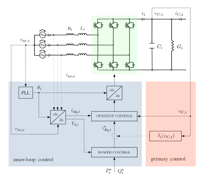
Figure 1: Control architecture of a three-phase voltage source converter that interfaces an ac subsystem—characterized by a three–phase input voltage $v_{ac,i}(t)$—to an hvdc network—characterized by an ingoing dc current $i_{C,i}(t)$. Bold lines represent electrical connections, while dashed lines represent signal connections [16].

As detailed above, the inner-loop control scheme is based on an appropriate $dq$ representation of the ac-side dynamics of the VSC, which for balanced operating conditions is given by the following second order dynamical system [17]:

$$L_{i}\dot{I}_{d,i} =-R_{i}I_{d,i}+L_{i}\omega_{i}I_{q,i}-d_{d,i}v_{C,i}+V_{d,i}$$ (II.2)

$$L_{i}\dot{I}_{q,i} =-L_{i}\omega_{i}I_{d,i}-R_{i}I_{q,i}-d_{q,i}v_{C,i}+V_{q,i}$$

where $I_{d,i}\in\mathbb{R}$ and $I_{q,i}\in\mathbb{R}$ denote the direct and quadrature currents, $v_{C,i}\in\mathbb{R}_{+}$ denotes the dc voltage, $d_{d,i}\in\mathbb{R}$ and $d_{q,i}\in\mathbb{R}$ denote the direct and quadrature duty ratios, $V_{d,i}\in\mathbb{R}$ and $V_{q,i}\in\mathbb{R}$ denote the direct and quadrature input voltages, $L_{i}\in\mathbb{R}_{+}$ and $R_{i}\in\mathbb{R}_{+}$ denote the (balanced) inductance and the resistance respectively. Moreover, the dc voltage dynamics can be described by the following scalar dynamical system:

$$C_{i}\dot{v}_{C,i}=-G_{i}v_{C,i}+i_{i}+i_{C,i},\quad i_{i}:=d_{d,i}I_{d,i}+d_{q,i}I_{q,i},$$ (II.3)

where $i_{C,i}\in\mathbb{R}$ denotes the current coming from the dc network, $i_{i}$ denotes the dc current injection via the VSC, $C_{i}\in\mathbb{R}_{+}$ and $G_{i}\in\mathbb{R}_{+}$ denote the capacitance and the conductance respectively. For a characterization of the power injections we consider the standard definitions of instantaneous active and reactive power associated to the ac-side of the VSC, which are given by [20, 21]:

$$P_{i} :=V_{d,i}I_{d,i}+V_{q,i}I_{q,i},\quad Q_{i}:=V_{q,i}I_{d,i}-V_{d,i}I_{q,i},$$ (II.4)

while the dc power associated to the dc-side is given by:

$$P_{\mathrm{DC},i}:=v_{C,i}i_{i}.$$ (II.5)

We now make two standard assumptions on the design of the inner-loop controllers.

Assumption II.1

$V_{q,i}=V_{q,i}^{\star}=0,\quad\forall t\geq 0.$

Assumption II.2

All inner-loop controllers are characterized by stable current control schemes. Moreover, the employed schemes guarantee instantaneous and exact tracking of the desired currents.

Assumption II.1 can be legitimized by appropriate design of the PLL mechanism, which is demanded to fix the $dq$ transformation angle so that the quadrature voltage is always kept zero after very small transients. Since a PLL usually operates in a range of a few $ms$, which is smaller than the time scale at which the power loop evolves, these transients can be neglected.
Similarly, Assumption II.2 can be legitimized by an appropriate design of the current control scheme so that the resulting closed-loop system is internally stable and has a very large bandwidth compared to the dc voltage dynamics and to the outer loops. In fact, tracking of the currents is usually achieved in $10-50$ $ms$, while dc voltage dynamics and outer loops evolve at a much slower time-scale [1].

Under Assumption II.1 and Assumption II.2, from the stationary equations of the currents dynamics expressed by (II.2), i.e. for $\dot{I}_{d,i}^{\star}=0$, $\dot{I}_{q,i}^{\star}=0$, we have that

$$d_{d,i}^{\star} =\frac{1}{v_{C,i}}\left(-R_{i}I_{d,i}^{\star}+L_{i}\omega_{i}I_{q,i}^{\star}+V_{d,i}^{\star}\right),\quad d_{q,i}^{\star}=\frac{1}{v_{C,i}}\left(-L_{i}\omega_{i}I_{d,i}^{\star}-R_{i}I_{q,i}^{\star}\right),$$ (II.6)

where $I_{d,i}^{\star}$ and $I_{q,i}^{\star}$ denote the controlled $dq$ currents (the dynamics of which are neglected under Assumption II.2), while $V_{d,i}^{\star}$ denotes the corresponding direct voltage on the ac-side of the VSC. By substituting (II.6) into (II.3) and recalling the definition of active power provided in (II.4), the controlled dc current can thus be expressed as

$$i_{i}^{\star}=\frac{V_{d,i}^{\star}I_{d,i}^{\star}-R_{i}(I_{d,i}^{\star})^{2}-R_{i}(I_{q,i}^{\star})^{2}}{v_{C,i}}=\frac{P_{i}^{\star}-D_{i}^{\star}}{v_{C,i}},$$ (II.7)

where

$$P_{i}^{\star}:=V_{d,i}^{\star}I^{\star}_{d,i},\quad D_{i}^{\star}:=R_{i}\left[(I_{d,i}^{\star})^{2}+(I_{q,i}^{\star})^{2}\right]$$ (II.8)

denote respectively the controlled active power on the ac-side and the power dissipated internally by the converter. We then make a further assumption.

Assumption II.3

$D_{i}^{\star}=0.$

Assumption II.3 can be justified by the high efficiency of the converter, i.e. by the small values of the balanced three-phase resistance $R$, which yield $D_{i}^{\star}\approx 0$. Hence, by replacing (II.7) into (II.3) and using the definitions (II.8), we obtain the following scalar dynamical system [21]:

$$C_{i}\dot{v}_{C,i}=-G_{i}v_{C,i}+\frac{V^{\star}_{d,i}}{v_{C,i}}I^{\star}_{d,i}+i_{C,i}$$ (II.9)

with $i\sim\mathcal{E}_{P}\cup\mathcal{E}_{V}$, which describes the dc-side dynamics of a VSC under assumptions II.1, II.2 and II.3. By taking (II.9) as a point of departure, we next derive the dynamics of the current-controlled VSCs in closed-loop with the outer power control.

If the unit is a PQ unit, the current references are simply determined by the outer power loop via (II.4) with constant active power $P_{j}^{\mathrm{ref}}$ and reactive power $Q_{j}^{\mathrm{ref}}$, which by noting that $V_{q,j}^{\star}=0$, are given by:

$$I_{d,j}^{\star}=\frac{P^{\mathrm{ref}}_{j}}{V^{\star}_{d,j}},\quad I_{q,j}^{\star}=-\frac{Q^{\mathrm{ref}}_{j}}{V^{\star}_{d,j}},$$ (II.10)

with $j\sim\mathcal{E}_{P}$, which replaced into (II.9) gives

$$C_{j}\dot{v}_{C,j}=-G_{j}v_{C,j}+u_{j}(v_{C,j})+i_{C,j}.$$ (II.11)

with the new current variable $u_{j}$ and the dc voltage $v_{C,j}$ verifying the hyperbolic constraint $P^{\mathrm{ref}}_{j}=v_{C,j}u_{j}$, $j\sim\mathcal{E}_{P}$. Hence, a PQ unit can be approximated, with respect to its power behavior, by a constant power device of value $P^{\mathrm{ref}}_{P,j}:=P^{\mathrm{ref}}_{j}$, see also Fig. 2(a). On the other hand, if the converter unit is a voltage-controlled unit, the current references are modified according to the primary control strategy. A common approach in this scenario is to introduce an additional deviation (also called droop) in the direct current reference—obtained from the outer power loop—as a function of the dc voltage, while keeping the calculation of the reference of the quadrature current unchanged:

$$I_{d,k}^{\star}=\frac{P_{k}^{\mathrm{ref}}}{V_{d,k}^{\star}}+\delta_{k}(v_{C,k}),\quad I_{q,k}^{\star}=-\frac{Q_{k}^{\mathrm{ref}}}{V_{d,k}^{\star}},$$ (II.12)

with $k\sim\mathcal{E}_{V}$ and where $\delta_{k}(v_{C,k})$ represents the state-dependent contribution provided by the primary control. We propose the primary control law:

$$\delta_{k}(v_{C,k})=\frac{1}{V_{d,k}^{\star}}\left(\mu_{P,k}+\mu_{I,k}v_{C,k}+\mu_{Z,k}v^{2}_{C,k}\right),$$ (II.13)

with $k\sim\mathcal{E}_{V}$ and where $\mu_{P,k}$, $\mu_{I,k},\mu_{Z,k}\in\mathbb{R}$ are free control parameters. By replacing (II.12)-(II.13) into (II.9), we obtain

$$C_{k}\dot{v}_{C,k}=-(G_{k}-\mu_{Z,k})v_{C,j}+\mu_{I,k}+u_{k}(v_{C,k})+i_{C,k},$$ (II.14)

with the new current variable $u_{k}$ and the dc voltage $v_{C,k}$ verifying the hyperbolic constraint $P^{\mathrm{ref}}_{k}+\mu_{P,k}=v_{C,k}u_{k}$, $k\sim\mathcal{E}_{V}$. Moreover, with Assumption II.3 the injected dc power is given by:

$$P_{\mathrm{DC},k}(v_{C,k})=P^{\mathrm{ref}}_{V,k}+\mu_{I,k}v_{C,k}+\mu_{Z,k}v_{C,k}^{2},$$ (II.15)

with

$$P^{\mathrm{ref}}_{V,k}:=P_{k}^{\mathrm{ref}}+\mu_{P,k},$$

from which follows, with the control law (II.13), that a voltage-controlled unit can be approximated, with respect to its power behavior, by a ZIP model, i.e. the parallel connection of a constant impedance (Z), a constant current source/sink (I) and a constant power device (P). More precisely—see also Fig. 2(b)—the parameters $P^{\mathrm{ref}}_{{V},k}$, $\mu_{I,k}$ and $\mu_{Z,k}$ represent the constant power, constant current and constant impedance of the ZIP model.

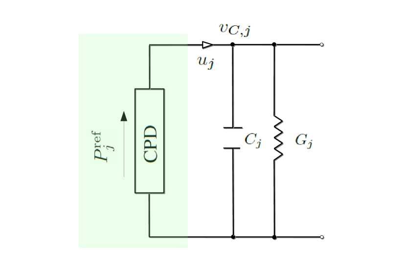
(a) Equivalent circuit scheme for PQ units.

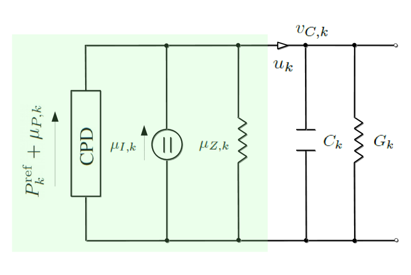
(b) Equivalent circuit scheme for voltage-controlled units.

Figure 2: Equivalent circuit schemes of the converter units with constant power devices (CPDs), under Assumption II.2.

Finally, the dynamics of the PQ units can be represented by the following scalar systems:

$$C_{j}\dot{v}_{C,j} =-G_{j}v_{C,j}+u_{j}+i_{C,j},$$

$$0 =P^{\mathrm{ref}}_{{P},j}-v_{C,j}u_{j},$$

while for the dynamics of the voltage-controlled units we have:

$$C_{k}\dot{v}_{C,k} =-(G_{k}-\mu_{Z,k})v_{C,k}+\mu_{I,k}+u_{k}+i_{C,k},$$

$$0 =P^{\mathrm{ref}}_{{V},k}-v_{C,k}u_{k},$$

with $j\sim\mathcal{E}_{{P}},k\sim\mathcal{E}_{{V}}$ and where $v_{C,j},v_{C,k}\in\mathbb{R}_{+}$ denote the voltages across the capacitors, $i_{C,j},i_{C,k}\in\mathbb{R}$ denote the network currents, $u_{j},u_{k}\in\mathbb{R}$ denote the currents flowing into the constant power devices, $G_{j}\in\mathbb{R}_{+}$, $G_{k}\in\mathbb{R}_{+}$, $C_{j}\in\mathbb{R}_{+}$, $C_{k}\in\mathbb{R}_{+}$ denote the conductances and capacitances. The aggregated model is then given by:

$$\begin{bmatrix}C_{P}\dot{v}_{{P}}\\ C_{V}\dot{v}_{{V}}\end{bmatrix}=- \begin{bmatrix}G_{{P}}&0\\ 0&G_{{V}}+G_{Z}\end{bmatrix}\begin{bmatrix}v_{{P}}\\ v_{{V}}\end{bmatrix}+\begin{bmatrix}u_{{P}}\\ u_{{V}}\end{bmatrix}+\begin{bmatrix}0\\ \bar{u}_{V}\end{bmatrix}+\begin{bmatrix}i_{{P}}\\ i_{V}\end{bmatrix},$$ (II.16)

together with the algebraic constraints:

$$P^{\mathrm{ref}}_{{P},j} =v_{{P},j}u_{{P},i},\quad P^{\mathrm{ref}}_{{V},k}=v_{{V},k}u_{{V},k},$$

with $i\sim\mathcal{E}_{{P}},k\sim\mathcal{E}_{{V}}$ and the following definitions.

• State vectors

  $$v_{{P}}:=\mbox{col}(v_{C,j})\in\mathbb{R}^{\mathsf{p}},\quad v_{{V}}:=\mbox{col}(v_{C,k})\in\mathbb{R}^{\mathsf{v}}.$$

• Network ingoing currents

  $$i_{{P}}:=\mbox{col}(i_{C,j})\in\mathbb{R}^{\mathsf{p}},\quad i_{{V}}:=\mbox{col}(i_{C,k})\in\mathbb{R}^{\mathsf{v}}.$$

• Units ingoing currents

  $$u_{{P}}:=\mbox{col}(u_{j})\in\mathbb{R}^{\mathsf{p}},\quad u_{{V}}:=\mbox{col}(u_{k})\in\mathbb{R}^{\mathsf{v}}.$$

• External sources $\bar{u}_{V}:=\mbox{col}(\mu_{I,k})\in\mathbb{R}^{\mathsf{v}}$.

• Matrices

  $$C_{{P}}: =\mathrm{diag}\{C_{j}\}\in\mathbb{R}^{\mathsf{p}\times\mathsf{p}},\;\;C_{{V}}:=\mathrm{diag}\{C_{k}\}\in\mathbb{R}^{\mathsf{v}\times\mathsf{v}},$$

  $$G_{{P}}: =\mathrm{diag}\{G_{j}\}\in\mathbb{R}^{\mathsf{p}\times\mathsf{p}},\;\;G_{{V}}:=\mathrm{diag}\{G_{k}\}\in\mathbb{R}^{\mathsf{v}\times\mathsf{v}},\;\;G_{Z}:=\mathrm{diag}\{-\mu_{Z,k}\}\in\mathbb{R}^{\mathsf{v}\times\mathsf{v}}.\;\;$$

II-C Interconnected model

For the model derivation of the hvdc network we assume that the dc transmission lines can be described by standard, single-cell $\pi$-models. However, it should be noted that at each converter node the line capacitors will result in a parallel connection with the output capacitor of the converter [22]. Hence, the capacitors at the dc output of the converter can be replaced by equivalent capacitors and the transmission lines described by simpler $RL$ circuits, for which it is straightforward to obtain the aggregated model [11]:

$$L_{T}\dot{i}_{T} =-R_{T}i_{T}+v_{T},$$ (II.17)

with $i_{T}:=\mathrm{col}(i_{T,i})\in\mathbb{R}^{\mathsf{t}}$, $v_{T}:=\mathrm{col}(v_{T,i})\in\mathbb{R}^{\mathsf{t}}$ denoting the currents through and the voltages across the lines and $L_{T}:=\mathrm{col}(L_{T,i})\in\mathbb{R}^{\mathsf{t}\times\mathsf{t}}$, $R_{T}:=\mathrm{col}(R_{T,i})\in\mathbb{R}^{\mathsf{t}\times\mathsf{t}}$ denoting the inductance and resistance matrices. In order to obtain the reduced, interconnected model of the hvdc transmission system under Assumption II.2, we need to consider the interconnection laws determined by the incidence matrix (II.1). Let us define the node and edge vectors:

$$V_{n}:=\begin{bmatrix}\mathcal{V}_{{P}}\\ \mathcal{V}_{{V}}\\ 0\end{bmatrix}\in\mathbb{R}^{\mathsf{c}+1},\;V_{e}:=\begin{bmatrix}v_{{P}}\\ v_{{V}}\\ v_{T}\end{bmatrix}\in\mathbb{R}^{\mathsf{m}},\;I_{e}:=\begin{bmatrix}i_{{P}}\\ i_{{V}}\\ i_{T}\end{bmatrix}\in\mathbb{R}^{\mathsf{m}}.$$

By using the definition of the incidence matrix (II.1) together with the Kirchhoff’s current and voltage laws given by [23, 24]:

$$\mathcal{B}I_{e}=0,\qquad V_{e}=\mathcal{B}^{\top}V_{n},$$

we obtain:

$$i_{{P}} =-\mathcal{B}_{{P}}v_{{P}},\quad i_{{V}}=-\mathcal{B}_{{V}}v_{{V}},\quad v_{T}=\mathcal{B}_{{P}}^{\top}v_{P}+\mathcal{B}_{{V}}^{\top}v_{V}.$$ (II.18)

Replacing $i_{P}$ and $i_{V}$ in (II.16) and $v_{T}$ in (II.17), leads to the interconnected model:

$$\begin{bmatrix}C_{P}\dot{v}_{{P}}\\ C_{V}\dot{v}_{{V}}\\ L_{T}\dot{i}_{T}\end{bmatrix}= \begin{bmatrix}-G_{{P}}&0&-\mathcal{B}_{{P}}\\ 0&-G_{{V}}&-\mathcal{B}_{{V}}\\ \mathcal{B}_{{P}}^{\top}&\mathcal{B}_{{P}}^{\top}&-G_{Z}\end{bmatrix}\begin{bmatrix}v_{{P}}\\ v_{{V}}\\ i_{T}\end{bmatrix}+\begin{bmatrix}u_{{P}}\\ u_{{V}}\\ 0\end{bmatrix}+\begin{bmatrix}0\\ \bar{u}_{V}\\ 0\end{bmatrix},$$ (II.19)

together with the algebraic constraints:

$$P^{\mathrm{ref}}_{{P},j}=v_{{P},j}u_{{P},j},\quad P^{\mathrm{ref}}_{{V},k}=v_{{V},k}u_{{V},k},$$ (II.20)

with $i\sim\mathcal{E}_{{P}},k\sim\mathcal{E}_{{V}}$.

Remark II.4

With the choice

$$\mu_{P,k}=0,\quad\mu_{I,k}=d_{k}v_{C}^{\mathrm{nom}},\quad\mu_{Z,k}=-d_{k},$$

the primary control (II.13) reduces to:

$$\delta_{k}(v_{C,k})=-\frac{d_{k}}{V_{d,k}^{\star}}(v_{C,k}-v_{C}^{\mathrm{nom}}),$$

while the injected current is simply given by

$$i_{k}^{\star}=\frac{V_{d,k}^{\star}}{v_{C,k}}I_{d,k}^{\star}=\frac{P_{k}^{\mathrm{ref}}}{v_{C,k}}-d_{k}(v_{C}^{\mathrm{nom}}-v_{C,k}),$$

with $k\sim\mathcal{E}_{V}$. This is exactly the conventional, widely diffused, voltage droop control [25, 6, 2], where $d_{k}$ is called droop coefficient and $v^{\mathrm{nom}}_{C}$ is the nominal voltage of the hvdc system. The conventional droop control can be interpreted as an appropriate parallel connection of a current source with an impedance, which is put in parallel with a constant power device, thus resulting in a ZIP model. A similar model is encountered in [4] and should be contrasted with the models provided in [3, 7], where the contribution of the constant power device is absent.

Remark II.5

A peculiarity of hvdc transmission systems with respect to generalized dc grids is the absence of traditional loads. Nevertheless, the aggregated model of the converter units (II.16) can be still employed for the modeling of dc grids with no loss of generality, under the assumption that loads can be represented either by PQ units (constant power loads) or by voltage-controlled units with assigned parameters (ZIP loads). This model should be contrasted with the linear models adopted in [7, 3] for dc grids, where loads are modeled as constant current sinks.

III A REDUCED MODEL FOR GENERAL DC SYSTEMS WITH SHORT LINES CONFIGURATIONS

Since hvdc transmission systems are usually characterized by very long, i.e. dominantly inductive, transmission lines, there is no clear time-scale separation between the dynamics of the power converters and the dynamics of the hvdc network. This fact should be contrasted with traditional power systems—where a time-scale separation typically holds because of the very slow dynamics of generation and loads compared to those of transmission lines [26]—and microgrids—where a time-scale separation is justified by the short length, and consequently fast dynamics, of the lines [27]. Nevertheless, as mentioned in Remark II.5, the model (II.19)-(II.20) is suitable for the description of a very general class of dc grids. By taking this model as a point of departure, we thus introduce a reduced model that is particularly appropriate for the description of a special class of dc grids, i.e. dc grids with short lines configurations. This class includes, among the others, the widely popular case of dc microgrids [28] and the case of hvdc transmission systems with back-to-back configurations [29]. For these configurations, we can then make the following assumption.

Assumption III.1

The dynamics of the dc transmission lines evolve on a time-scale that is much faster than the time-scale at which the dynamics of the voltage capacitors evolve.

Under Assumption III.1, (II.17) reduces to:

$$i_{T}\equiv i_{T}^{\star}=G_{T}v_{T},$$ (III.1)

where $i_{T}^{\star}$ is the steady-state vector of the line currents and $G_{T}:=R_{T}^{-1}$ the conductance matrix of the transmission lines. By replacing the expression (III.1) into (II.19) we finally obtain:

$$\begin{bmatrix}C_{P}\dot{v}_{{P}}\\ C_{V}\dot{v}_{{V}}\end{bmatrix}=- \begin{bmatrix}\mathcal{L}_{{P}}+G_{{P}}&\mathcal{L}_{m}\\ \mathcal{L}_{m}^{\top}&\mathcal{L}_{{V}}+G_{{V}}+G_{Z}\end{bmatrix}\begin{bmatrix}v_{{P}}\\ v_{{V}}\end{bmatrix}+\begin{bmatrix}u_{{P}}\\ u_{{V}}\end{bmatrix}+\begin{bmatrix}0\\ \bar{u}_{V}\end{bmatrix},$$ (III.2)

together with the algebraic constraints (II.20) and where we defined

$$\mathcal{L}_{P}: =\mathcal{B}_{{P}}G_{L}\mathcal{B}_{{P}}^{\top},\quad\mathcal{L}_{m}:=\mathcal{B}_{{P}}G_{L}\mathcal{B}_{{V}}^{\top},\quad\mathcal{L}_{V}:=\mathcal{B}_{{V}}G_{L}\mathcal{B}_{{V}}^{\top}.$$

Remark III.2

The matrix:

$$\mathcal{L}:=\begin{bmatrix}\mathcal{L}_{{P}}&\mathcal{L}_{m}\\ \mathcal{L}_{m}^{\top}&\mathcal{L}_{{V}}\end{bmatrix}\in\mathbb{R}^{\mathsf{c}\times\mathsf{c}}$$

is the Laplacian matrix associated to the weighted undirected graph $\bar{\mathcal{G}}^{w}$, obtained from the (unweighted directed) graph $\mathcal{G}^{\uparrow}$ that describes the hvdc transmission system by: 1) eliminating the reference node and all edges connected to it; 2) assigning as weights of the edges corresponding to transmission lines the values of their conductances. Similar definitions are also encountered in [3, 7].

IV CONDITIONS FOR EXISTENCE OF AN EQUILIBRIUM POINT

From an electrical point of view, the reduced system (II.19)-(II.20) is a linear $RLC$ circuit, where at each node a constant power device is attached. It has been observed in experiments and simulations that the presence of constant power devices may seriously affect the dynamics of these circuits hindering the achievement of a constant, stable behavior of the state variables—the dc voltages in the present case [30, 31, 10, 32]. A first objective is thus to determine conditions on the free control parameters of the system (II.19)-(II.20) for the existence of an equilibrium point. Before presenting the main result of this section, we make an important observation: since the steady-state of the system (II.19)-(II.20) is equivalent to the steady-state of the system (III.2)-(II.20), the analysis of existence of an equilibrium point follows verbatim. Based on this consideration, in the present section we will only consider the system (III.2)-(II.20), bearing in mind the the same results hold for the system (II.19)-(II.20). To simplify the notation, we define

$$P_{{P}}^{\mathrm{ref}}: =\mathrm{col}(P_{{P},j}^{\mathrm{ref}})\in\mathbb{R}^{\mathsf{p}},\quad R_{P}:=\mathcal{L}_{P}+G_{P}\in\mathbb{R}^{\mathsf{p}\times\mathsf{p}},$$ (IV.1)

$$P_{{V}}^{\mathrm{ref}}: =\mathrm{col}(P_{{V},k}^{\mathrm{ref}})\in\mathbb{R}^{\mathsf{v}},\quad R_{V}:=\mathcal{L}_{V}+G_{V}+G_{Z}\in\mathbb{R}^{\mathsf{v}\times\mathsf{v}}.$$

Furthermore, we recall the following lemma, the proof of which can be found in [10].

Lemma IV.1

Consider $m$ quadratic equations of the form $f_{i}:\mathbb{R}^{n}\rightarrow\mathbb{R}$,

$$f_{i}(x):=\frac{1}{2}x^{\top}\mathcal{A}_{i}x+x^{\top}\mathcal{B}_{i},\qquad i\in[1,m],$$ (IV.2)

where $\mathcal{A}_{i}=\mathcal{A}_{i}^{\top}\in\mathbb{R}^{n\times n}$, $\mathcal{B}_{i}\in\mathbb{R}^{n}$, $c_{i}\in\mathbb{R}$ and define:

$$\mathcal{A}(T): =\sum_{i=1}^{m}t_{i}\mathcal{A}_{i},\quad\mathcal{B}(T):=\sum_{i=1}^{m}t_{i}\mathcal{B}_{i},\quad\mathcal{C}(T):=\sum_{i=1}^{m}t_{i}c_{i}.$$

If the following LMI

$$\Upsilon(T):=\begin{bmatrix}\mathcal{A}(T)&\mathcal{B}(T)\\ \mathcal{B}^{\top}(T)&-2\mathcal{C}(T)\end{bmatrix}>0,$$

is feasible, then the equations

$$f_{i}(x)=c_{i},\qquad i\in[1,m],$$ (IV.3)

have no solution.

We are now ready to formulate the following proposition, that establishes necessary, control parameter-dependent, conditions for the existence of equilibria of the system (III.2)-(II.20).

Proposition IV.2

Consider the system (III.2)-(II.20), for some given $P_{{P}}^{\mathrm{ref}}\in\mathbb{R}^{\mathsf{p}}$, $P_{{V}}^{\mathrm{ref}}\in\mathbb{R}^{\mathsf{v}}$. Suppose that there exist two diagonal matrices $T_{{P}}\in\mathbb{R}^{\mathsf{p}\times\mathsf{p}}$ and $T_{{V}}\in\mathbb{R}^{\mathsf{v}\times\mathsf{v}}$ such that:

$$\Upsilon(T_{P},T_{V})>0,$$ (IV.4)

with

$$\Upsilon:=\begin{bmatrix}T_{{P}}R_{P}+R_{P}T_{{P}}&T_{{P}}\mathcal{L}_{m}+\mathcal{L}_{m}^{\top}T_{{V}}&0\\ \star&T_{{V}}R_{V}+R_{V}T_{{V}}&-T_{{V}}\bar{u}_{V}\\ \star&\star&-2(\mathsf{1}_{\mathsf{p}}^{\top}T_{P}P_{{P}}^{\mathrm{ref}}+\mathsf{1}_{\mathsf{v}}^{\top}T_{V}P_{{V}}^{\mathrm{ref}})\end{bmatrix},$$

where $P_{P}^{\star}$, $P_{V}^{\star}$, $R_{P}$ and $R_{V}$ are defined in (IV.1). Then the system (III.2)-(II.20) does not admit an equilibrium point.

Proof:

First of all, by setting the left-hand of the differential equations in (III.2) to zero and using (IV.1), we have:

$$0= -R_{P}v_{{P}}^{\star}-\mathcal{L}_{m}v_{{V}}^{\star}+u_{{P}}^{\star},$$

$$0= -\mathcal{L}_{m}^{\top}v_{{P}}^{\star}-R_{V}v_{{V}}^{\star}+u_{{V}}^{\star}+\bar{u}_{V}.$$

Left-multiplying the first and second set of equations by $v_{{P},j}^{\star}$ and $v_{{V},k}^{\star}$ respectively, with $j\sim\mathcal{E}_{{P}}$, $k\sim\mathcal{E}_{{V}}$, we get

$$P_{{P},j}^{\mathrm{ref}} =v_{{P},j}^{\star}R^{\top}_{P,j}v_{{P}}^{\star}+v_{{P},j}^{\star}\mathcal{L}^{\top}_{m,j}v_{{V}}^{\star},$$

$$P_{{V},k}^{\mathrm{ref}} =v_{{V},k}^{\star}\mathcal{L}_{m,k}v_{{P}}^{\star}+v_{{V},k}^{\star}R_{V,k}^{\top}v_{{V}}^{\star}-v_{{V},k}^{\star}\bar{u}_{V,k},$$

which, after some manipulations, gives

$$c_{i} =\frac{1}{2}(v^{\star})^{\top}\mathcal{A}_{i}v^{\star}+(v^{\star})^{\top}\mathcal{B}_{i},$$ (IV.5)

with $i\sim\mathcal{E}_{P}\cup\mathcal{E}_{V}$, $v^{\star}:=\mathrm{col}(v_{{P}}^{\star},v_{{V}}^{\star})\in\mathbb{R}^{\mathsf{c}}$ and

$$\mathcal{A}_{i}: =e_{i}e_{i}^{\top}\begin{bmatrix}R_{P}&\mathcal{L}_{m}\\ \mathcal{L}_{m}^{\top}&R_{V}\end{bmatrix}+\begin{bmatrix}R_{P}&\mathcal{L}_{m}^{\top}\\ \mathcal{L}_{m}&R_{V}\end{bmatrix}e_{i}e_{i}^{\top},\quad\mathcal{B}_{i}:=e_{i}e_{i}^{\top}\begin{bmatrix}0\\ \bar{u}_{V}\end{bmatrix},\quad c_{i}:=e_{i}^{\top}\begin{bmatrix}P_{P}^{\mathrm{ref}}\\ P_{V}^{\mathrm{ref}}\end{bmatrix}.$$

Let consider the map $f(v^{\star}):\mathbb{R}^{\mathsf{c}}\rightarrow\mathbb{R}^{\mathsf{c}}$ with components

$$f_{i}(v^{\star})=\frac{1}{2}(v^{\star})^{\top}\mathcal{A}_{i}v^{\star},$$

with $i\sim\mathcal{E}_{P}\cup\mathcal{E}_{V}$ and denote by $F$ the image of $\mathbb{R}^{\mathsf{c}}$ under this map. The problem of solvability of such equations can be formulated as in Lemma IV.1, i.e. if the LMI (IV.4) holds, then $\mathrm{col}(c_{i}^{\star})$ is not in $F$, thus completing the proof. $\Box\Box\Box$

Remark IV.3

Note that the feasibility of the LMI (IV.4) depends on the system topology reflected in the Laplacian matrix $\mathcal{L}$ and on the system parameters, among which $G_{Z}$, $\bar{u}_{V}$ and $P_{{V}}^{\mathrm{ref}}$ are free (primary) control parameters. Since the feasibility condition is only necessary for the existence of equilibria for (II.19), it is of interest to determine regions for these parameters that imply non-existence of an equilibrium point.

V CONDITIONS FOR POWER SHARING

As already discussed, another control objective of primary control is the achievement of power sharing among the voltage-controlled units. This property consists in guaranteeing an appropriate (proportional) power distribution among these units in steady-state. We next show that is possible to reformulate such a control objective as a set of quadratic constraints on the equilibrium point, assuming that it exists. Since it is a steady-state property, the same observation done in Section IV applies, which means that the results obtained for the system (III.2)-(II.20) also hold for the system (II.19)-(II.20). We introduce the following definition.

Definition V.1

Let be $v^{\star}:=(v_{{P}}^{\star},v_{{V}}^{\star})\in\mathbb{R}^{\mathsf{c}}$ and $P_{\mathrm{DC},V}(v^{\star}):=\mathrm{col}({P}_{\mathrm{DC},k}(v^{\star}_{C,k}))\in\mathbb{R}^{\mathsf{v}}$ respectively an equilibrium point for the system (III.2)-(II.20) and the collection of injected powers as defined by (II.15), and let be $\Gamma:=\mathrm{diag}\{\gamma_{k}\}\in\mathbb{R}^{\mathsf{v}\times\mathsf{v}},$ a positive definite matrix. Then $v^{\star}$ is said to possess the power sharing property with respect to $\Gamma$ if:

$$\Gamma P_{\mathrm{DC},V}(v^{\star})=\mathsf{1}_{\mathsf{v}}.$$ (V.1)

Then we have the following lemma.

Lemma V.2

Let $v^{\star}=(v_{{P}}^{\star},v_{{V}}^{\star})\in\mathbb{R}^{\mathsf{c}}$ be an equilibrium point for (III.2)-(II.20) and $\Gamma:=\mathrm{diag}\{\gamma_{k}\}\in\mathbb{R}^{\mathsf{v}\times\mathsf{v}}$ a positive definite matrix. Then $v^{\star}$ possesses the power sharing property with respect to $\Gamma$ if an only if the quadratic equations

$$\frac{1}{2}(v^{\star})^{\top}\mathcal{A}^{\mathrm{ps}}_{k}v^{\star}+(\mathcal{B}^{\mathrm{ps}}_{k})^{\top}v^{\star}=p^{\mathrm{ps}}_{k},$$ (V.2)

with $k\sim\mathcal{E}_{V}$ and where:

$$\mathcal{A}^{\mathrm{ps}}_{k}: =2\begin{bmatrix}0&0\\ 0&\Gamma G_{Z}\end{bmatrix}e_{k}e_{k}^{\top},\quad\mathcal{B}^{\mathrm{ps}}_{k}:=\begin{bmatrix}0\\ \Gamma\bar{u}_{V}\end{bmatrix}e_{k}e_{k}^{\top},\quad p^{\mathrm{ps}}_{k}:=e_{k}^{\top}\begin{bmatrix}0\\ \Gamma P_{{V}}^{\mathrm{ref}},\end{bmatrix}$$

admit a solution.

Proof:

From (V.1) we have that by definition:

$$\gamma_{k}P^{\mathrm{ref}}_{\mathrm{DC},k}(v_{C,k})=1,$$

with $k\sim\mathcal{E}_{V}$, which by recalling (II.15), is equivalent to:

$$\gamma_{k}(P_{{V},k}^{\mathrm{ref}}+\mu_{I,k}v_{C,k}+\mu_{Z,k}v_{C,k}^{2})=1.$$

After some straightforward manipulations, the above equalities can be rewritten as (V.2), completing the proof. $\Box\Box\Box$

An immediate implication of this lemma is given in the following proposition, which establishes necessary conditions for the existence of an equilibrium point that verifies the power sharing property.

Proposition V.3

Consider the system (III.2)-(II.20), for some given $P_{{P}}^{\mathrm{ref}}$, $P_{{V}}^{\mathrm{ref}}$ and $\Gamma$. Suppose that there exist three diagonal matrices $T_{{P}}\in\mathbb{R}^{\mathsf{p}\times\mathsf{p}}$, $T_{{V}}\in\mathbb{R}^{\mathsf{v}\times\mathsf{v}},T_{V}^{\mathrm{ps}}\in\mathbb{R}^{\mathsf{v}\times\mathsf{v}}$, such that:

$$\Upsilon(T_{P},T_{V})+\Upsilon_{\mathrm{ps}}(T_{V}^{\mathrm{ps}})>0,$$ (V.3)

with

$$\Upsilon_{\mathrm{ps}}:=\begin{bmatrix}0&0&0\\ \star&2T_{V}^{\mathrm{ps}}\Gamma G_{Z}&T_{V}^{\mathrm{ps}}\Gamma\bar{u}_{V}\\ \star&\star&-2T_{V}^{\mathrm{ps}}(\mathsf{1}_{\mathsf{v}}-\Gamma P_{{V}}^{\mathrm{ref}})\end{bmatrix}.$$

Then the system (III.2)-(II.20) does not admit an equilibrium point that verifies the power sharing property.

Proof:

The proof is similar to the proof of Proposition IV.2. By using Lemma V.2 the power sharing constraints can be indeed rewritten as quadratic equations, similarly to (IV.5). Hence, it suffices to apply Lemma IV.1 to the quadratic equations (IV.5), (V.2) to complete the proof. $\Box\Box\Box$

VI CONDITIONS FOR LOCAL ASYMPTOTIC STABILITY

We now present a result on stability of a given equilibrium point for the system (II.19)-(II.20). The result is obtained by applying Lyapunov’s first method.

Proposition VI.1

Consider the system (II.19)-(II.20) and assume that $v^{\star}=(v_{{P}}^{\star},v_{{V}}^{\star},i_{T}^{\star})\in\mathbb{R}^{\mathsf{m}}$ is an equilibrium point. Let

$$G_{{P}}^{\star}: =\mathrm{diag}\left\{\frac{P_{{P},j}^{\mathrm{ref}}}{(v_{{P},j}^{\star})^{2}}\right\}\in\mathbb{R}^{\mathsf{p}\times\mathsf{p}},\quad G_{{V}}^{\star}:=\mathrm{diag}\left\{\frac{P_{{V},k}^{\mathrm{ref}}}{(v_{{V},k}^{\star})^{2}}\right\}\in\mathbb{R}^{\mathsf{v}\times\mathsf{v}},$$ (VI.1)

and

$$J(v^{\star}):=-\begin{bmatrix}-C_{{P}}^{-1}(G_{P}+G_{{P}}^{\star})&0&-C_{{P}}^{-1}\mathcal{B}_{P}\\ 0&-C_{{V}}^{-1}(G_{V}+G_{{V}}^{\star})&-C_{V}^{-1}\mathcal{B}_{V}\\ L_{T}^{-1}\mathcal{B}_{P}^{\top}&L_{T}^{-1}\mathcal{B}_{V}^{\top}&-L_{T}^{-1}R_{T}\end{bmatrix}.$$

Then if:

• all eigenvalues $\lambda_{i}$ of $J$ are such that

  $$\mathfrak{Re}\{\lambda_{i}\left[J(v^{\star})\right]\}<0,$$

  the equilibrium point $v^{\star}$ is locally asymptotically stable;

• there exists at least one eigenvalue $\lambda_{i}$ of $J$ such that

  $$\mathfrak{Re}\{\lambda_{i}\left[J(v^{\star})\right]\}>0,$$

  the equilibrium point $v^{\star}$ is unstable.

Proof:

The first-order approximation of the system (II.19)-(II.20) around $v^{\star}$ is given by:

$$\begin{bmatrix}C_{P}\dot{v}_{{P}}\\ C_{V}\dot{v}_{{V}}\\ L_{T}\dot{i}_{T}\end{bmatrix}= \begin{bmatrix}-G_{P}&0&-\mathcal{B}_{P}\\ 0&-G_{V}&-\mathcal{B}_{V}\\ \mathcal{B}_{P}^{\top}&\mathcal{B}_{V}^{\top}&-R_{T}\end{bmatrix}\begin{bmatrix}v_{{P}}\\ v_{{V}}\\ i_{T}\end{bmatrix}+\begin{bmatrix}\frac{\partial i_{{P}}}{\partial v_{{P}}}\big{|}_{v^{\star}}&0&0\\ 0&\frac{\partial i_{{V}}}{\partial v_{{V}}}\big{|}_{v^{\star}}&0\\ 0&0&0\end{bmatrix}\begin{bmatrix}v_{P}\\ v_{V}\\ i_{T}\end{bmatrix}$$ (VI.2)

Differentiating (II.20) with respect to $v_{{P}}$, $v_{{V}}$, yields:

$$0_{\mathsf{p}\times\mathsf{p}} =\frac{\partial i_{{P}}}{\partial v_{{P}}}\cdot\mathrm{diag}\{v_{{P},j}\}+\mathrm{diag}\{i_{{P},j}\},\quad 0_{\mathsf{v}\times\mathsf{v}}=\frac{\partial i_{{V}}}{\partial v_{{V}}}\cdot\mathrm{diag}\{v_{{V},k}\}+\mathrm{diag}\{i_{{V},k}\}.$$

By using (VI.1), it follows that

$$\frac{\partial i_{{P}}}{\partial v_{{P}}}\bigg{|}_{v^{\star}}=-G_{{P}}^{\star},\quad\frac{\partial i_{{V}}}{\partial v_{{V}}}\bigg{|}_{v^{\star}}=-G_{{V}}^{\star}.$$

The proof is completed by replacing into (VI.2) and invoking Lyapunov’s first method. $\Box\Box\Box$

VII AN ILLUSTRATIVE EXAMPLE

In order to validate the results on existence of equilibria and power sharing for the system (II.19)-(II.20) we next provide an illustrative example. Namely, we consider the four-terminal hvdc transmission system depicted in Fig. 3, the parameters of which are given in Table I.

TABLE I: System parameters.

	Value		Value		Value		Value		Value
$G_{i}$	$0$ $\Omega^{-1}$	$P_{V,1}^{\star}$	$30$ $MW$	$P_{P,2}^{\star}$	$-20$ $MW$	$P_{V,3}^{\star}$	$9$ $MW$	$P_{P,4}^{\star}$	$-24$ $MW$
$C_{i}$	$20$ $\mu F$	$G_{12}$	$0.1$ $\Omega^{-1}$	$G_{14}$	$0.15$ $\Omega^{-1}$	$G_{23}$	$0.11$ $\Omega^{-1}$	$G_{24}$	$0.08$ $\Omega^{-1}$

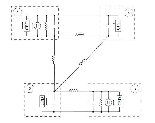
Figure 3: Four-terminal hvdc transmission system.

Since $\mathsf{c}=\mathsf{t}=4$, the graph associated to the hvdc system has $\mathsf{n}=4+1=5$ nodes and $\mathsf{m}=4+4=8$ edges. We then make the following assumptions.

• Terminal 1 and Terminal 3 are equipped with primary control, from which it follows that there are $\mathsf{p}=2$ PQ units and $\mathsf{v}=2$ voltage-controlled units. More precisely we take

  $$\delta_{k}(v_{C,k})=-\frac{d_{k}}{V_{d,k}^{\star}}(v_{C,k}-v_{C}^{\mathrm{nom}}),\quad k=\{1,3\}.$$

  This is the well-known voltage droop control, where $d_{k}$ is a free control parameter, while $v_{C}^{\mathrm{nom}}$ is the nominal voltage of the hvdc system, see also Remark II.4.

• The power has to be shared equally among terminal 1 and terminal 3, from which it follows that $\Gamma=\mathbb{I}_{2}$ in Definition V.1.

The next results are obtained by investigating the feasibility of the LMIs (IV.4), (V.3) as a function of the free control parameters $d_{1}$ and $d_{3}$. For this purpose, CVX, a package for specifying and solving convex programs, has been used to solve the semidefinite programming feasibility problem [33]. By using a gridding approach, the regions of the (positive) parameters that guarantee feasibility (yellow) and unfeasibility (blue) of the LMI (IV.4) are shown in Fig. 4, while in Fig. 5 the same is done with respect to the LMI (V.3). We deduce that a necessary condition for the existence of an equilibrium point is that the control parameters are chosen inside the blue region of Fig. 4. Similarly, a necessary condition for the existence of an equilibrium point that further possesses the power sharing property is that the control parameters are chosen inside the blue region of Fig. 5.

Figure 4: Feasibility regions of the LMI (IV.4) on the plane $(d_{1},d_{3})$ of droop control parameters. Regions are yellow-coloured if the LMI is feasible and blue-coloured if the LMI is unfeasible.

Figure 5: Feasibility regions of the LMI (V.3) on the plane $(d_{1},d_{3})$ of droop control parameters. Regions are yellow-coloured if the LMI is feasible and blue-coloured if the LMI is unfeasible.

VIII CONCLUSIONS AND FUTURE WORKS

In this paper, a new nonlinear model for primary control analysis and design has been derived. Primary control laws are described by equivalent ZIP models, which include the standard voltage droop control as a special case. A necessary condition for the existence of equilibria in the form of an LMI—which depends on the parameters of the controllers—is established, thus showing that an inappropriate choice of the latter may lead to non-existence of equilibria for the closed-loop system. The same approach is extended to the problem of existence of equilibria that verify a pre-specified power sharing property. The obtained necessary conditions can be helpful to system operators to tune their controllers such that regions where the closed-loop system will definitely not admit a stationary operating point are excluded. In that regard, the present paper is a first, fundamental stepping stone towards the development of a better understanding of how existence of stationary solutions of hvdc systems are affected by the system parameters, in particular the network impedances and controller gains. A final contribution consists in the establishment of conditions of local asymptotic stability of a given equilibrium point. The obtained results are illustrated on a four-terminal example.

Starting from the obtained model, future research will concern various aspects. First of all, a better understanding of how the feasibility of the LMIs are affected by the parameters is necessary. A first consideration is that the established conditions, besides on the controllers parameters, also depends on the network topology and the dissipation via the Laplacian matrix induced by the electrical network. This suggests that the location of the voltage-controlled units, as well as the network impedances, play an important role on the existence of equilibria for the system. Similarly, it is of interest to understand in which measure the values of Z, I and P components of the equivalent ZIP mode affect the LMIs, in order to provide guidelines for the design of primary controllers. Furthermore, the possibility to combine the obtained necessary conditions with related (sufficient) conditions from the literature, e.g. in [34], is very interesting and timely. Other possible developments will focus on the establishment of necessary (possibly sufficient) conditions for the existence of equilibria in different scenarios: small deviations from the nominal voltage [9, 4]; power unit outages [4]; linear three-phase, ac circuit, investigating the role played by reactive power [32].

IX ACKNOWLEDGMENTS

The authors acknowledge the support of: the Future Renewable Electric Energy Distribution Management Center (FREEDM), a National Science Foundation supported Engineering Research Center, under grant NSF EEC-0812121; the Ministry of Education and Science of Russian Federation (Project14.Z50.31.0031); the European Union’s Horizon 2020 research and innovation programme under the Marie Sklodowska-Curie grant agreement No. 734832.

References

- [1] A. Egea-Alvarez, J. Beerten, D. V. Hertem, and O. Gomis-Bellmunt, “Hierarchical power control of multiterminal HVDC grids,” Electric Power Systems Research, vol. 121, pp. 207 – 215, 2015.
- [2] T. K. Vrana, J. Beerten, R. Belmans, and O. B. Fosso, “A classification of DC node voltage control methods for HVDC grids,” Electric Power Systems Research, vol. 103, pp. 137 – 144, 2013.
- [3] M. Andreasson, M. Nazari, D. V. Dimarogonas, H. Sandberg, K. H. Johansson, and M. Ghandhari, “Distributed voltage and current control of multi-terminal high-voltage direct current transmission systems,” IFAC Proceedings Volumes, vol. 47, no. 3, pp. 11910–11916, 2014.
- [4] J. Beerten and R. Belmans, “Analysis of power sharing and voltage deviations in droop-controlled DC grids,” Power Systems, IEEE Transactions on, vol. 28, no. 4, pp. 4588 – 4597, 2013.
- [5] S. Shah, R. Hassan, and J. Sun, “HVDC transmission system architectures and control - a review,” in Control and Modeling for Power Electronics, 2013 IEEE 14th Workshop on, pp. 1–8, June 2013.
- [6] T. Haileselassie, T. Undeland, and K. Uhlen, “Multiterminal HVDC for offshore windfarms – control strategy,” European Power Electronics and Drives Association, 2009.
- [7] J. Zhao and F. Dorfler, “Distributed control and optimization in DC microgrids,” Automatica, vol. 61, pp. 18 – 26, 2015.
- [8] N. Monshizadeh, C. D. Persis, A. van der Schaft, and J. M. A. Scherpen, “A networked reduced model for electrical networks with constant power loads,” CoRR, vol. abs/1512.08250, 2015.
- [9] J. W. Simpson-Porco, F. Dörfler, and F. Bullo, “On resistive networks of constant-power devices,” Circuits and Systems II: Express Briefs, IEEE Transactions on, vol. 62, pp. 811–815, Aug 2015.
- [10] N. Barabanov, R. Ortega, R. Grino, and B. Polyak, “On existence and stability of equilibria of linear time-invariant systems with constant power loads,” Circuits and Systems I: Regular Papers, IEEE Transactions on, vol. PP, no. 99, pp. 1–8, 2015.
- [11] D. Zonetti, R. Ortega, and A. Benchaib, “Modeling and control of HVDC transmission systems from theory to practice and back,” Control Engineering Practice, vol. 45, pp. 133 – 146, 2015.
- [12] F. Dörfler and F. Bullo, “Kron reduction of graphs with applications to electrical networks,” IEEE Transactions on Circuits and Systems I: Regular Papers, vol. 60, no. 1, pp. 150–163, 2013.
- [13] A. Yazdani and R. Iravani, Voltage–Sourced Controlled Power Converters – Modeling, Control and Applications. Wiley IEEE, 2010.
- [14] C. Stijn, Steady-state and dynamic modelling of VSC HVDC systems for power system Simulation. PhD thesis, PhD dissertation, Katholieke University Leuven, Belgium, 2010.
- [15] R. Best, Phase-Locked Loops. Professional Engineering, Mcgraw-hill, 2003.
- [16] D. Zonetti, Energy-based modelling and control of electric power systems with guaranteed stability properties. PhD thesis, Université Paris-Saclay, 2016.
- [17] V. Blasko and V. Kaura, “A new mathematical model and control of a three-phase ac-dc voltage source converter,” IEEE Transactions on Power Electronics, vol. 12, pp. 116–123, Jan 1997.
- [18] L. Xu, B. Andersen, and P. Cartwright, “Control of vsc transmission systems under unbalanced network conditions,” in Transmission and Distribution Conference and Exposition, 2003 IEEE PES, vol. 2, pp. 626–632 vol.2, Sept 2003.
- [19] T. Lee, “Input-output linearization and zero-dynamics control of three-phase AC/DC voltage-source converters,” IEEE Tranactions on Power Electronics, vol. 18, pp. 11–22, Jan 2003.
- [20] H. Akagi, Instantaneous Power Theory and Applications to Power Conditioning. Newark: Wiley, 2007.
- [21] R. Teodorescu, M. Liserre, and P. Rodríguez, Grid Converters for Photovoltaic and Wind Power Systems. John Wiley and Sons, Ltd, 2011.
- [22] S. Fiaz, D. Zonetti, R. Ortega, J. Scherpen, and A. van der Schaft, “A port-Hamiltonian approach to power network modeling and analysis,” European Journal of Control, vol. 19, no. 6, pp. 477 – 485, 2013.
- [23] A. van der Schaft, “Characterization and partial synthesis of the behavior of resistive circuits at their terminals,” Systems & Control Letters, vol. 59, no. 7, pp. 423 – 428, 2010.
- [24] S. Fiaz, D. Zonetti, R. Ortega, J. Scherpen, and A. van der Schaft, “A port-Hamiltonian approach to power network modeling and analysis,” European Journal of Control, vol. 19, no. 6, pp. 477 – 485, 2013.
- [25] E. Prieto-Araujo, F. Bianchi, A. Junyent-Ferré, and O. Gomis-Bellmunt, “Methodology for droop control dynamic analysis of multiterminal vsc-hvdc grids for offshore wind farms,” Power Delivery, IEEE Transactions on, vol. 26, pp. 2476–2485, Oct 2011.
- [26] P. Sauer, “Time-scale features and their applications in electric power system dynamic modeling and analysis,” in American Control Conference (ACC), 2011, pp. 4155–4159, June 2011.
- [27] J. Schiffer, D. Zonetti, R. Ortega, A. M. Stanković, T. Sezi, and J. Raisch, “A survey on modeling of microgrids—from fundamental physics to phasors and voltage sources,” Automatica, vol. 74, pp. 135–150, 2016.
- [28] Y. Ito, Y. Zhongqing, and H. Akagi, “DC microgrid based distribution power generation system,” in Power Electronics and Motion Control Conference, 2004. IPEMC 2004. The 4th International, vol. 3, pp. 1740–1745, IEEE, 2004.
- [29] M. Bucher, R. Wiget, G. Andersson, and C. Franck, “Multiterminal HVDC Networks – what is the preferred topology?,” Power Delivery, IEEE Transactions on, vol. 29, pp. 406–413, Feb 2014.
- [30] M. Belkhayat, R. Cooley, and A. Witulski, “Large signal stability criteria for distributed systems with constant power loads,” in Power Electronics Specialists Conference, 1995. PESC ’95 Record., 26th Annual IEEE, vol. 2, pp. 1333–1338 vol.2, Jun 1995.
- [31] A. Kwasinski and C. N. Onwuchekwa, “Dynamic behavior and stabilization of DC microgrids with instantaneous constant-power loads,” Power Electronics, IEEE Transactions on, vol. 26, pp. 822–834, 2011.
- [32] S. Sanchez, R. Ortega, R. Grino, G. Bergna, and M. Molinas, “Conditions for existence of equilibria of systems with constant power loads,” Circuits and Systems I: Regular Papers, IEEE Transactions on, vol. 61, no. 7, pp. 2204–2211, 2014.
- [33] M. Grant and S. Boyd, “CVX: Matlab software for disciplined convex programming, version 2.1.”
- [34] S. Bolognani and S. Zampieri, “On the existence and linear approximation of the power flow solution in power distribution networks,” IEEE Transactions on Power Systems, vol. 31, pp. 163–172, Jan 2016.