NuSTAR observations of the supergiant X-ray pulsar IGR J18027-2016: accretion from the stellar wind and possible cyclotron absorption line

Abstract

We report on the first focused hard X-ray view of the absorbed supergiant system IGR J18027-2016 performed with the NuSTAR observatory. The pulsations are clearly detected with a period of $P_{\rm spin}=139.866(1)$ s and a pulse fraction of about 50-60% at energies from 3 to 80 keV. The source demonstrates an approximately constant X-ray luminosity on a time scale of more than dozen years with an average spin-down rate of $\dot{P}\simeq 6\times 10^{-10}$ s s^-1. This behaviour of the pulsar can be explained in terms of the wind accretion model in the settling regime. The detailed spectral analysis at energies above 10 keV was performed for the first time and revealed a possible cyclotron absorption feature at energy $\sim 23$ keV. This energy corresponds to the magnetic field $B\simeq 3\times 10^{12}$ G at the surface of the neutron star, which is typical for X-ray pulsars.

1 Introduction

IGR J18027-2016 was discovered by the INTEGRAL observatory during deep observations of the Galactic Center region as a faint persistent hard X-ray source (Revnivtsev et al., 2004). Follow-up observations performed with the XMM-Newton observatory in soft X-rays allowed for an improvement in the determination of the source position, enabling near-infrared observations with the NTT/ESO telescope and establishing the nature of its companion as a supergiant star of B1Ib type (Torrejón et al., 2010) at a distance of 12.4 kpc. Mason et al. (2011) classified the optical star as B0-B1 I, which is broadly in agreement with the above mentioned type.

Using archival data from the BeppoSAX observatory, Augello et al. (2003) revealed that the serendipitous source SAX J1802.7-2017 is spatially associated with IGR J18027-2016. These authors showed that this source is an X-ray pulsar with a spin period of 139.6 s, residing in a binary system with an orbital period of 4.6 days. Later, the orbital parameters of the system were improved by Hill et al. (2005) and Falanga et al. (2015).

The average spectrum of IGR J18027-2016, measured in a wide energy band (Lutovinov et al., 2005), demonstrates a cutoff at high energies, which is typical for X-ray pulsars (see, e.g., Filippova et al., 2005). In addition, a relatively high absorption value, $N_{\rm H}=6.8\times 10^{22}$ cm^-2, was revealed at low energies (Hill et al., 2005), and the source was classified as an absorbed binary system with a supergiant companion (Walter et al., 2015). No search for a cyclotron absorption line and no pulse phase resolved spectroscopic study for IGR J18027-2016 has been performed to date.

In this paper we report on results of observations of IGR J18027-2016 collected with the NuSTAR observatory and Swift/XRT telescope in Aug 2015. The main purpose of these observations was to characterize the broadband spectrum with high accuracy and to search for a cyclotron absorption line.

2 Observations and data reduction

The Nuclear Spectroscopic Telescope Array (NuSTAR) has two identical X-ray telescope modules, each equipped with independent mirror systems and focal plane detector units, also referred to as FPMA and FPMB (Harrison et al., 2013). The unique multilayered coating of the grazing-incidence Wolter-I optics provides X-ray imaging in the energy range $3-79$ keV with an angular resolution of 18^′′ (FWHM) and 58^′′ (HPD). Each telescope has a field-of-view (FOV) of $\sim 13^{\prime}\times 13^{\prime}$. CdZnTe pixel detectors of FPMA and FPMB provide spectral resolution of 400 eV (FWHM) at 10 keV.

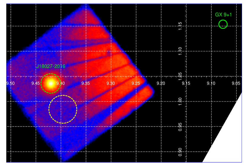
Figure 1: The NuSTAR image of IGR J18027-2016 in the $3-79$ keV energy band obtained with FPMA module (the picture for another module FPMB is practically identical). Green and yellow dashed circles denote source and background extraction regions, respectively. The ghost-ray (GR) contamination is revealed by a pattern of characteristic radial streaks in the image. The GR photons originate from GX 9+1, whose position is marked by the solid green circle. The white grid indicates the Galactic coordinate system in degrees.

IGR J18027-2016 was observed with NuSTAR on August 27, 2015 from MJD 57,261.0141 to 57,261.9922 (ObsID 30101049002, the total data span length is about 78 ks) during Cycle 1 of the Guest Observer Program with a total on-target exposure of $\sim 36$ ks ($\sim 32.6$ ks after the dead-time correction and GX 9+1 flare removal, see below). The presence of bright nearby sources can contaminate the NuSTAR observations due to the aperture stray light – unfocused X-rays reaching the NuSTAR detectors. The contamination that we see is often called ghost-rays (GR), which are photons that are reflected from only upper or lower X-ray mirror sections (so-called single scattering photons, see, e.g., Wik et al. 2014; Krivonos et al. 2014; Mori et al. 2015). The bright low-mass X-ray binary system GX 9+1 is located in close proximity to IGR J18027-2016 (at an angular distance of 21.5^′). Therefore, initially (at the observation planning stage), we checked for possible contamination of GR photons from this source to the useful signal. According to NuSTAR’s experience with GRs from the very bright system 4U 1630-47 (Bodaghee et al., 2014), the direct GRs are observed within a $\sim 20$^′ radius circle, which made observations of IGR J18027-2016 possible. Indeed, Fig. 1 demonstrates that there is no a strong GR contamination from the persistent emission of GX 9+1 at the position of IGR J18027-2016. However, a strong X-ray flare was detected in the light curve of IGR J18027-2016. Timing and spectral characteristics of this event are typical for Type I X-ray bursts observed from some accreting neutron stars. The burst is also clearly present in a light curve extracted from the background data, which are fully dominated by the GX 9+1 GR contamination. Therefore, we suggest that the burst originated from GX 9+1, and we removed the corresponding part of the data from the following analysis. Note that the exposure accumulated during the burst (300 sec in total) is too short to identify a characteristic pattern of ghost-rays.

Figure 2: Distribution of periods obtained for $5\times 10^{4}$ trial light curves (histogram) and its best-fit approximation with the Gaussian (solid line).

We processed the raw observational data to produce cleaned event files for the FPMA and FPMB modules using the standard NuSTAR Data Analysis Software (NuSTARDAS) v1.6.0 provided under HEASOFT v6.19 with CALDB version 20160502. Using the nuproducts routine, we extracted source counts for spectral and timing analysis within 70^′′ of the centroid position (dashed green circle in Fig. 1), which corresponds to $\sim 80\%$ of the enclosed PSF fraction (Madsen et al., 2015). Taking into account possible GR contamination, we extracted the background spectrum and light curves in the region with a radius of 100^′′(dashed yellow circle), located at nearly same distance from GX 9+1 (its position is indicated by the solid green circle in Fig. 1). Finally, after background subtraction the total number of registered photons from the source is about $\simeq 1.36\times 10^{5}$ for both modules.

Figure 3: Pulse profiles of IGR J18027-2016 in five energy bands 3–6, 6–10, 10–20, 20–40, and 40–79 keV (from top to bottom). The profiles are normalized by the mean flux in each energy band and plotted twice for clarity.

For timing analysis and pulse phase-resolved spectroscopy, the data were corrected for the barycenter of the Solar System with the barycorr command and for the binary system motion using orbital parameters from Falanga et al. (2015).

The Swift/XRT instrument observed IGR J18027-2016 simultaneously with the NuSTAR observatory on August 27, 2015 (MJD $57261.6525-57261.7159$, ObsID 00081660001) with a total exposure of $\sim 2$ ks. The Swift/XRT data were used to supplement the NuSTAR data in the soft energy band and to better determine the level of absorption. These data were reduced using appropriate software.

All of the spectra were then grouped to have more than 20 counts per bin using the grppha tool from the HEAsoft package. The final data analysis (timing and spectral) was performed with the FTOOLS 6.7 software package.

3 Timing analysis

The NuSTAR observatory provides data with very good time and energy resolution, allowing us to investigate temporal properties of IGR J18027-2016 at energies above 10 keV in detail for the first time. In general, the source light curve measured by NuSTAR demonstrates two types of variability on time scales longer than the pulse period and shorter than the orbital period: smooth changes of the source intensity during the observation and relatively quick variations (up to $25-30$%) on the time scale of several thousand seconds. It can be naturally expected that both types of variations are connected with gradual changes of the stellar wind density over the orbit of the neutron star and its local inhomogeneities.

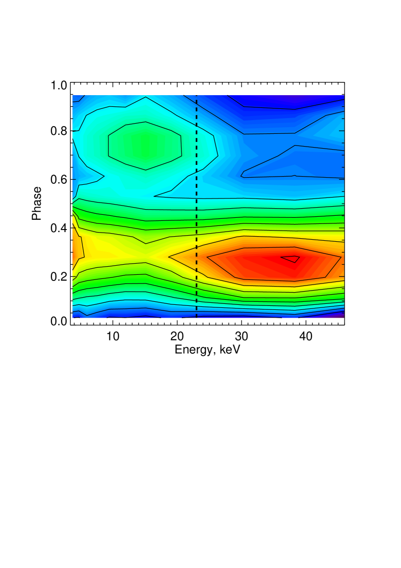
Figure 4: “Energy – pulse phase” distribution of intensity for IGR J18027-2016. The dashed vertical line shows the position of the cyclotron line revealed in the source spectrum. The profiles were also normalized by the mean flux in each energy band. Solid contours represent levels of the equal normalized flux from 0.5 to 1.85 with steps of 0.15.

The pulse period and its uncertainty were determined using the combined light curve from both modules FPMA and FPMB (see Krivonos et al., 2015, for the description of the procedure) in the wide energy band (3–79 keV) with 1 s time bins and corrected both for the motion of Earth around Sun and the neutron star in the binary system. In general, a correct determination of the pulse period, signal amplitude, their uncertainties using the epoch folding technique is not trivial task and different approaches have been proposed (see, e.g. Leahy, 1987; Larsson, 1996; D’Aì et al., 2011). Here, to estimate an uncertainty on the pulse period we generated $5\times 10^{4}$ trial light curves (using the statistics from the original one, provided with the nuproducts package) and determined the pulse period value in each of them using the epoch folding technique. We used the efsearch procedure from the FTOOLS package with 24 trial profile phase bins. The distribution of periods obtained has a smooth shape, which can be well describe with a Gaussian profile (see Fig. 2). The mean and standard deviation corresponds approximately to the proper pulse period and its $1\sigma$ uncertainty, respectively (see, e.g., Boldin, Tsygankov, & Lutovinov, 2013, for details). The final value of the pulse period obtained by this analysis is $P_{\rm spin}=139.866\pm 0.001$ s, where the uncertainty corresponds to $1\sigma$ confidence level.

The obtained value of $P_{\rm spin}$ is larger by about $\simeq 0.25$ s compared with the previous measurements made with the BeppoSAX and XMM-Newton observatories (Hill et al., 2005), resulting in the mean spin-down rate of $\dot{P}\simeq 6\times 10^{-10}$ s s^-1.

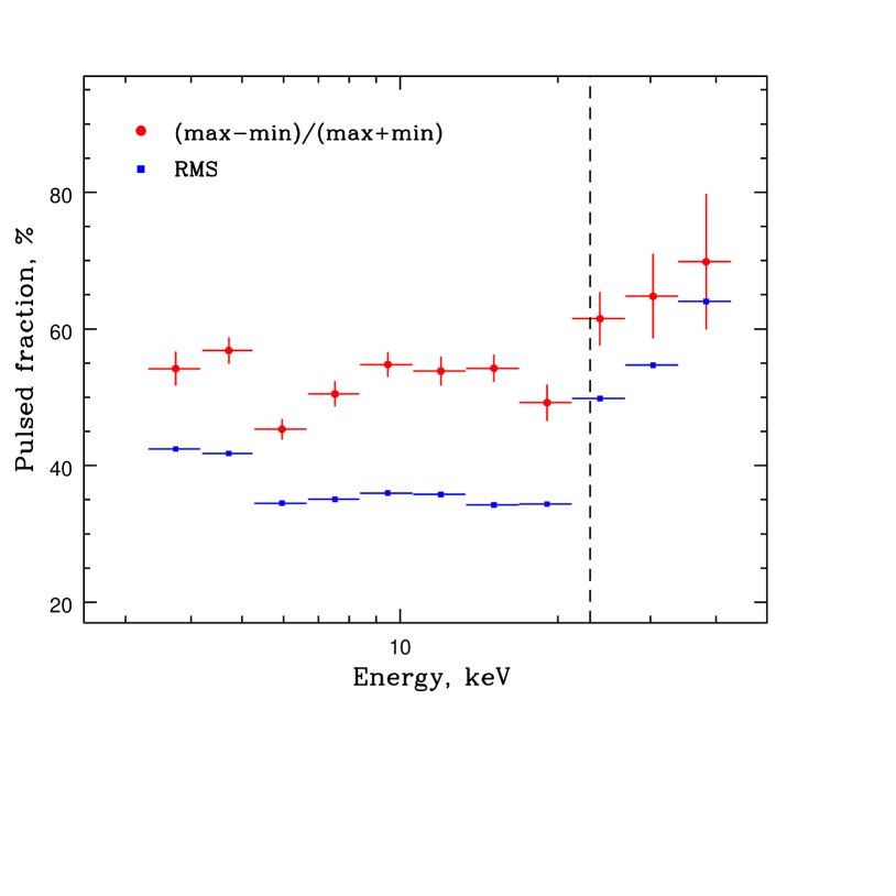
Figure 5: Dependence of the pulsed fraction of IGR J18027-2016 on energy calculated in two different ways (see text for details). The dashed line shows the position of the cyclotron line that may be present in the source spectrum.

The pulse profiles in five different energy bands 3–6, 6–10, 10–20, 20–40, and 40–79 keV (from top to bottom) are shown in Fig. 3. In all energy bands, it has a double peak shape with different relative intensities of the peaks.

The evolution of the pulse profile with energy can be illustrated by the “energy – pulse phase” distribution of the intensity made possible by NuSTAR’s energy resolution (see Fig. 4). These pulse profiles were also normalized by the mean flux in each energy band. Details of the technique of the construction of such a 2D-distribution are described by Lutovinov & Tsygankov (2009) and have already been successfully used in a number of works. From Fig. 4, it is clear that the second peak has its highest relative intensity between $\sim 10$ and $\sim 20$ keV. At higher energies, the first peak completely dominates the profile. It is important to note that these two energy ranges are divided by the possible cyclotron absorption line revealed in the source spectrum (see Section 4). Its position is shown with the dashed line in Fig. 4.

The pulsed fraction below the cyclotron line energy depends on energy only slightly with a value of 50–60% (see Fig. 5). At higher energies one can see the gradual increase of the pulsed fraction, typical for the majority of X-ray pulsars (Lutovinov & Tsygankov, 2009).

To avoid possible biases due to the pulse profile peculiarities or statistics, we used two different definitions of the pulsed fraction. The “standard” one is $\mathrm{PF}=(F_{\mathrm{max}}-F_{\mathrm{min}})/(F_{\mathrm{max}}+F_{\mathrm{min}})$, where $F_{\mathrm{max}}$ and $F_{\mathrm{min}}$ are maximum and minimum fluxes in the pulse profile, respectively. Red circles in Fig. 5 show the pulsed fraction defined by this manner. Another way to characterize the pulse profile intensity variations is to use the relative Root Mean Square (RMS), which can be calculated by the following equation:

$$RMS=\frac{\Big{(}\frac{1}{N}\sum_{i=1}^{N}(P_{i}-\langle P\rangle)^{2}\Big{)}^{\frac{1}{2}}}{\langle P\rangle},$$ (1)

where $P_{i}$ is the background-corrected count rate in a given bin of the pulse profile, $\langle P\rangle$ is the profile-averaged count rate, and $N$ is the total number of phase bins in the profile.

The overall behaviour of the pulsed fraction calculated using the different approaches agrees very well with the only difference being a slightly lower absolute value for the RMS (blue squares in Fig. 5). This dependence shows two distinct features: the increase of the pulsed fraction with energy and its peculiar change at $22-24$ keV. Note that there is another similar change of the pulsed fraction around 6-7 keV probably connected with the fluorescent iron emission line.

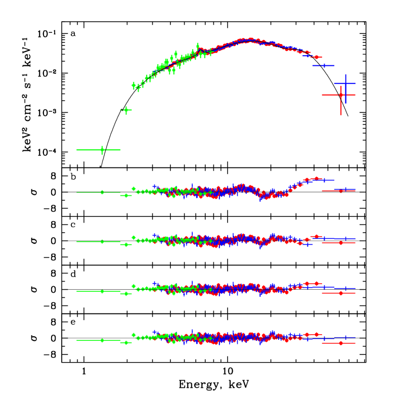
Figure 6: (a) Pulse phase averaged spectrum of IGR J18027-2016 obtained with the NuSTAR observatory and the Swift/XRT instrument. Red circles and blue crosses correspond to data from FPMA and FPMB, respectively; green points – to the XRT data. The black line shows the best fit model. (b-e) Residuals from different models (see text for details). The spectrum and residuals were rebinned in the figure to make the deviations more readily apparent.

4 Spectral analysis

Table 1: Best-fit parameters of the IGR J18027-2016 spectrum with different models.

Parameter	Comptt	Comptt+Gabs	PowHigh${}^{\mbox{\small a}}$	PowHigh+Gabs
$C1$	$1.014\pm 0.006$	$1.013\pm 0.006$	$1.013\pm 0.006$	$1.013\pm 0.006$
$C2$	$0.87\pm 0.04$	$0.86\pm 0.04$	$0.86\pm 0.04$	$0.86\pm 0.04$
$N_{\rm H}$, $\times 10^{22}$ cm-2	$3.55\pm 0.30$	$3.22\pm 0.30$	$3.36\pm 0.22$	$3.23\pm 0.21$
$kT_{\rm 0}$, keV	$0.61\pm 0.09$	$0.70\pm 0.09$	–	–
$kT$, keV	$5.91\pm 0.04$	$6.86\pm 0.08$	–	–
$\tau$	$7.59\pm 0.13$	$7.41\pm 0.14$	–	–
Photon index	–	–	$0.89\pm 0.02$	$0.87\pm 0.02$
$E_{\rm cut}$, keV	–	–	$12.49\pm 0.13$	$12.93\pm 0.25$
$E_{\rm fold}$, keV	–	–	$11.10\pm 0.18$	$11.56\pm 0.31$
$\tau_{\rm cycl}$	–	$0.53^{+0.08}_{-0.07}$	–	$0.16^{+0.07}_{-0.04}$
$E_{\rm cycl}$, keV	–	$24.26\pm 0.49$	–	$23.2\pm 1.0$
$\sigma_{\rm cycl}$, keV	–	$5.93^{+0.46}_{-0.42}$	–	$5.35^{+1.13}_{-0.75}$
$E_{\rm Fe}$, keV	$6.46\pm 0.03$	$6.45\pm 0.03$	$6.46\pm 0.03$	$6.46\pm 0.03$
$\sigma_{\rm Fe}$, keV	$0.2$ (fix)	$0.2$ (fix)	$0.2$ (fix)	$0.2$ (fix)
$EW$, eV	$106^{+23}_{-11}$	$121^{+29}_{-9}$	$117^{+13}_{-13}$	$118^{+12}_{-8}$
Flux (3–79 keV)${}^{\mbox{\small b}}$	$(1.695^{+0.010}_{-0.016})\times 10^{-10}$ erg s-1 cm-2
Luminosity (3–79 keV)${}^{\mbox{\small c}}$	$(3.107^{+0.019}_{-0.029})\times 10^{36}$ erg s-1
$\chi^{2}$ (d.o.f)	$1572.3(1127)$	$1229.1(1124)$	$1211.4(1127)$	$1172.5(1124)$

${}^{\mbox{\small a}}$	the powerlaw*highcut in the XSPEC package
${}^{\mbox{\small b}}$	measured flux
${}^{\mbox{\small c}}$	for a distance of 12.4 kpc (Torrejón et al., 2010)

The working energy range of the NuSTAR observatory (3–79 keV), and its unprecedented sensitivity at $>10$ keV makes the observatory an ideal instrument to search for cyclotron resonant scattering features (or, in other words, cyclotron absorption lines) in the spectra of X-ray pulsars (for more recent examples see, e.g., Bodaghee et al., 2016; Tsygankov et al., 2016). Moreover, the quality of the NuSTAR data is so high that the simple theoretical models usually used for the modelling of spectra of X-ray pulsars are often not able to approximate them satisfactorily, and we were met with this problem in the analysis of the IGR J18027-2016 spectrum.

As mentioned above, the spectrum of IGR J18027-2016 is typical for accreting X-ray pulsars. In particular, it demonstrates an exponential cutoff at high energies (Fig. 6a). Therefore, as a first step, we attempted to approximate it with several commonly used models: a power law with an exponential cutoff (cutoffpl in the XSPEC package), the NPEX model, the broken power law model (see, e.g., Hill et al., 2005), thermal inverse Comptonization (comptt in the XSPEC package), a power law with a high energy cutoff (powerlaw*highcut in the XSPEC package, White, Swank, & Holt 1983). To take into account the absorption in the system, the phabs model was used with the abundances from Anders & Grevesse (1989).

The source and background spectra from both the FPMA and FPMB modules of NuSTAR as well as from the Swift/XRT telescope were used for simultaneous fitting. To take into account the uncertainty in the instrument calibrations as well as the lack of full simultaneity of observations by NuSTAR and Swift (the former observed IGR J18027-2016 for nearly the whole day, while the latter observed for only 2 ks), cross-calibration constants between them were included in all spectral models (the $C1$ and $C2$ constants from Table 1 correspond to the cross-calibrations of the FPMB module and the XRT telescope to the FPMA module, respectively).

None of the models that we used describe the spectrum very well – typically, there are strong deviations at low energies and a depression around 20 keV with a complex shape. Moreover, two models (the broken power law and powerlaw*highcut) suffer from the abrupt breaks at the break and cutoff energies, respectively. This can lead to artificial narrow line features around these energies (see, e.g., Shtykovsky et al., 2016). Therefore, in the following analysis, we used the comptt model, which we consider to be the most reliable one.

Residuals between the source spectrum and the comptt model are shown in Fig. 6b. In comparison with other models, the comptt model approximates the soft part of the spectrum quite well and has a clear physical meaning. At the same time, Fig. 6b also shows a peculiarity in the spectrum – a deficit of photons around 20 keV, leading to a high $\chi^{2}$ value (Table 1).

To investigate this feature, we added an absorption component to the model in the form of the gabs model in the XSPEC package. It led to a significant improvement of the fit quality and $\chi^{2}$ value (Table 1). The corresponding residuals are shown in Fig. 6c, and the line centroid energy is $E_{cycl}\simeq 24.3$ keV. We interpret this absorption feature as a possible cyclotron absorption line. Two models, gabs and cyclabs in the XSPEC package, are usually used to approximate absorption lines. While both models provide an adequate description of the data, the cyclotron line energy derived from the gabs model is systematically higher by several keV than the energy derived from the cyclabs model (see, e.g., Tsygankov, Krivonos, & Lutovinov, 2012; Lutovinov et al., 2015). For IGR J18027-2016 and the cyclabs model, the cyclotron line energy would be $E_{cycl}\simeq 20.2$ keV. Note that some wavelike structure is still present in residuals, which can be attributed to physical causes or to inperfections in the model.

Besides the cyclotron absorption line, a strong emission feature associated with the fluorescent iron emission line is clearly visible near 6.4 keV. To take it into account, a corresponding component in the Gaussian form was added to the model. The final best fit parameters as well as the source intensity and luminosity are summarized in Table 1.

In order to trace the evolution of the source spectrum and its parameters over the pulse period, we carried out pulse phase-resolved spectroscopy. Taking into account the relative faintness of the source (its flux is only about 4-5 mCrab), the spin period was divided into four wide phase bins, roughly corresponding to the main and secondary peaks (Fig. 7). Such a division allows us to obtain spectra with good statistical quality at each phase and to determine the spectral parameters.

To approximate pulse phase-resolved spectra, we used the same model as for the averaged spectrum. However, the temperature of the seed photons $kT_{\rm 0}$ and the cyclotron line width were fixed to the values measured for the averaged spectrum because the temperature and width are poorly constrained due to the limitations of the spectral quality of the spectra. The column density was also fixed because only NuSTAR data (i.e., $>3$ keV) were used for the phase-resolved spectroscopy.

Variations of the spectral parameters over the pulse are shown in Fig. 7. For better visualization, the pulse profile of IGR J18027-2016 in a wide energy band 3-79 keV is plotted in each panel by the grey histogram. The continuum parameters ($kT$ and $\tau$) change slightly with the pulse phase, demonstrating a possible anticorrelation between them. In contrast, the cyclotron line energy demonstrates strong dependence of the pulse phase – in the main peak, it is around $E_{\rm cycl}\simeq 22$ keV, while in the secondary peak, it increases to $E_{\rm cycl}\simeq 28$ keV. Considering the relatively small width of the line ($\sim 5.5$ keV), it can lead to the wave-like structure in the residuals (see Fig. 6c).

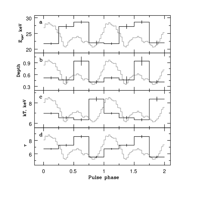
Figure 7: Spectral parameters of the comptonization model as a function of pulse phase. The black histogram in the panels represents: (a) cyclotron line energy, (b) cyclotron line depth, (c) temperature and (d) optical depth in the comptt model. The grey line in each panel shows the pulse profile in a wide energy range.

Finally, it is necessary to note that, formally, the best approximation of the IGR J18027-2016 spectrum is given when the powerlaw*highecut model is used for the continuum. This model was proposed by White, Swank, & Holt (1983) to approximate spectra of accreting X-ray pulsars. Despite the artificiality and presence of the abrupt break at the cutoff energy, it describes spectra obtained with the majority of X-ray observatories more or less adequately. The significant increase of the data quality in hard X-rays with the NuSTAR observatory raises a question about the physically based models for X-ray pulsar emission as, e.g., use of the powerlaw*highcut model can lead to artificial narrow absorption lines near the cutoff energy. Nevertheless, the IGR J18027-2016 spectrum is an example where this model works and describes it without leaving additional artificial features (see Table 1). The $\chi^{2}$ value for this model is significantly lower than for comptt and is comparable with comptt + gabs. However, even in this case, there is still some noticeable deficit of photons around 20 keV, which can be approximated by the adding of the gabs component to the model (see Fig. 6d,e). The improvement of the fit quality for this case is not so significant as for the comptt model. Therefore, we performed extensive Monte-Carlo simulations ($10^{5}$ trials) to estimate the significance of the line detection and found that it is about 4$\sigma$ for the powerlaw*highecut continuum model.

Results of the pulse phase-resolved spectroscopy for the powerlaw*highecut continuum model are shown in Fig. 8 in the same manner as in Fig. 7. The cyclotron line is not significantly detected in all phase bins, but its energy as a function of pulse phase is qualitatively similar to the behavior seen when using the comptonization continuum model – in the main peak, it is around $E_{\rm cycl}\simeq 20$ keV, while in the secondary peak, it increases up to $E_{\rm cycl}\simeq 30$ keV. Again, the cyclotron line width and column density were fixed to values from the pulse averaged spectrum.

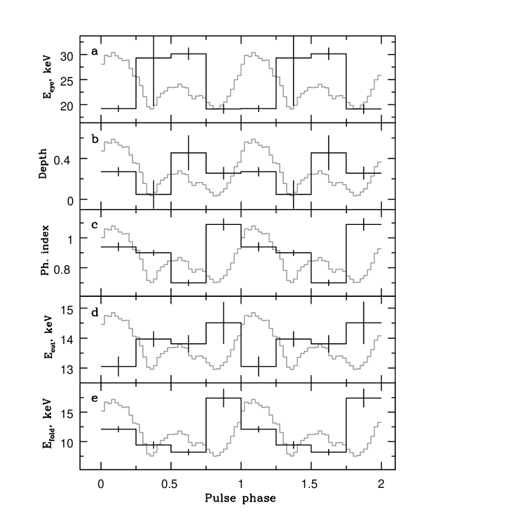
Figure 8: The same as in Fig. 7, but for the powerlaw*highcut model of the continuum. The black histogram in the panels represents: (a) cyclotron line energy, (b) cyclotron line depth, (c) photon index, (d) cutoff energy and (e) folding energy.

5 Discussion and conclusion

In this paper, we report results of the NuSTAR observations of the absorbed supergiant system IGR J18027-2016. They can be summarized as follows: 1) the system demonstrates approximately constant X-ray luminosity on a time scale of more than a dozen years; 2) during this time interval, the pulsar spun down with a rate of $\dot{P}\simeq 6\times 10^{-10}$ s s^-1; 3) the possible presence of a cyclotron absorption line at $\sim 23$ keV is found in the source X-ray spectrum.

The observed increase of the rotation period of the neutron star in IGR J18027-2016 can be explained in terms of the wind accretion model in a settling regime (Shakura et al., 2012, 2014), which can be realized for slowly rotating magnetized neutron stars at X-ray luminosities below $\sim 4\times 10^{36}$ erg s^-1. The observed stable X-ray luminosity suggests that the X-ray pulsar has reached its equilibrium period, which, in this model, depends on the binary orbital period $P_{b}$, the stellar wind velocity $v_{w}$, the neutron star magnetic moment $\mu$ and the mass accretion rate $\dot{M}$:

$$P_{eq}\simeq 940[\mathrm{s}]\mu_{30}^{12/11}\left(\frac{P_{b}}{10\mathrm{d}}\right)\dot{M}_{16}^{-4/11}v_{8}^{4}\,,$$ (2)

where the characteristic parameters are $\mu_{30}\equiv\mu/10^{30}[\mathrm{G\,cm}^{3}]$, $\dot{M}_{16}\equiv\dot{M}/10^{16}[\mathrm{g\,s}^{-1}]$, $v_{8}\equiv v_{w}/10^{8}[\mathrm{cm\,s}^{-1}]$. A very strong dependence on the wind velocity suggests that it is more reliable to estimate the wind velocity by inverting this formula. From the observed X-ray luminosity (see Table 1) we find $\dot{M}_{16}\simeq 3$, and assuming that the absorption feature is the cyclotron line, we find the neutron star dipole magnetic moment $\mu_{30}\simeq 2$. Therefore, assuming that the observed pulsar period is close to its equilibrium value, $P_{eq}=P_{spin}=139.6$ s, we can estimate the wind velocity $v_{8}\sim 0.7$. We stress that this estimate depends only very weakly on parameters ($\dot{M}$ and $\mu$ and other model-dependent numerical coefficients). Note that this rather low value is very close to the wind velocity measured in the prototypical persistent HMXB with OB supergiant Vela X-1 (, 2016), suggesting similarity between the two sources.

In the model of settling quasi-spherical accretion, the neutron star close to equilibrium can exhibit either spin-up or spin-down, depending on whether the actual $\dot{M}$ is above or below the critical mass accretion rate, $\dot{M}_{eq}$ (see Eq. (2) in Postnov et al. 2014). For the parameters of IGR J18027-2016, we find $\dot{M}_{eq}\simeq 3.6\times 10^{16}$ g s^-1, i.e. indeed spin-down of the neutron star is possible in this system. The observed value of the negative torque acting on the neutron star in IGR J18027-2016  $\dot{\omega}\simeq 2\times 10^{-13}$ rad s^-2, does not exceed the maximum possible negative torque, $\omega_{sd,max}\simeq 10^{-12}$ rad s^-2, for the parameters of IGR J18027-2016 (see Eq. (6) in Postnov et al. 2014). Thus, the observed steady-state spin-down is consistent with expectations from the settling accretion model.

As discussed in Section 4, the spectral analysis revealed the possible presence of a cyclotron absorption line in the spectrum of IGR J18027-2016 at energies of $\sim 23-24$ keV. An additional independent test for the existence of this feature comes from the timing properties of the source. Namely, the pulse profile and pulsed fraction dependencies on the energy have prominent features near the same energy. Particularly, the relative intensity of two peaks in the profile changes around 22-24 keV (see Fig. 4). Such behaviour was shown to be typical for another well known X-ray pulsar V 0332+53 with a well established cyclotron feature (Tsygankov et al., 2006). The observed non-monotonic dependence of the pulsed fraction on energy (see Fig. 5) is also typical for pulsars with cyclotron lines (Lutovinov & Tsygankov, 2009; Ferrigno et al., 2009). These additional observational facts indirectly support the presence of the cyclotron absorption line in the IGR J18027-2016 spectrum despite of its low significance for the powerlaw*highcut continuum model.

The measured X-ray luminosity in IGR J18027-2016, $L_{x}\simeq 3\times 10^{36}$ erg s^-1, suggests that accretion onto the neutron star occurs in the subcritical regime where the radiation plays a secondary role (see, e.g. Basko & Sunyaev, 1976; Mushtukov et al., 2015a). In this case, the accretion flow is decelerated in a collisionless shock formed at some height above the neutron star surface (Langer & Rappaport, 1982; Bykov & Krasil’shchikov, 2004). The formation of a cyclotron line downstream of the shock occurs in the resonance layer in the inhomogeneous magnetic field, so the line profile can be more complicated than the simple Doppler-broadened line (Zheleznyakov, 1996). For example, depending on the geometry, the line may have a flat bottom or show emission wings. The complex shape of the residuals shown in Fig. 6, which are obtained assuming a Gaussian form of the line, may suggest a complicated line profile or may be evidence for the presence of complicated magnetic field structure near the surface of the neutron star, as discussed, for example, in Mukherjee & Bhattacharya (2012). Moreover, as the optical thickness of the flow at the resonant energies is very high even at low mass accretion rate, the cyclotron line can be also formed in the accretion channel above the shock region (Mushtukov et al., 2015b). In this case, one would expect the cyclotron absorption feature to be redshifted relative to the actual cyclotron energy. This interesting result should be studied in the future with deeper observations.

References

- Anders & Grevesse (1989) Anders E., Grevesse N., 1989, GeCoA, 53, 197
- Augello et al. (2003) Augello G., Iaria R., Robba N. R., Di Salvo T., Burderi L., Lavagetto G., Stella L., 2003, ApJ, 596, L63
- Basko & Sunyaev (1976) Basko M. M., Sunyaev R. A., 1976, MNRAS, 175, 395
- Bodaghee et al. (2014) Bodaghee A., et al., 2014, ApJ, 791, 68
- Bodaghee et al. (2016) Bodaghee A., et al., 2016, ApJ, 823, 146
- Boldin, Tsygankov, & Lutovinov (2013) Boldin P. A., Tsygankov S. S., Lutovinov A. A., 2013, AstL, 39, 375
- Bykov & Krasil’shchikov (2004) Bykov A. M., Krasil’shchikov A. M., 2004, AstL, 30, 309
- D’Aì et al. (2011) D’Aì A., La Parola V., Cusumano G., Segreto A., Romano P., Vercellone S., Robba N. R., 2011, A&A, 529, A30
- Falanga et al. (2015) Falanga M., Bozzo E., Lutovinov A., Bonnet-Bidaud J. M., Fetisova Y., Puls J., 2015, A&A, 577, A130
- Ferrigno et al. (2009) Ferrigno C., Becker P. A., Segreto A., Mineo T., Santangelo A., 2009, A&A, 498, 825
- Filippova et al. (2005) Filippova E. V., Tsygankov S. S., Lutovinov A. A., Sunyaev R. A., 2005, AstL, 31, 729
- (12) Giménez-García A., et al., 2016, A&A, 591, A26
- Harrison et al. (2013) Harrison F. A., et al., 2013, ApJ, 770, 103
- Hill et al. (2005) Hill A. B., et al., 2005, A&A, 439, 255
- Krivonos et al. (2014) Krivonos R. A., et al., 2014, ApJ, 781, 107
- Krivonos et al. (2015) Krivonos R. A., et al., 2015, ApJ, 809, 140
- Langer & Rappaport (1982) Langer S. H., Rappaport S., 1982, ApJ, 257, 733
- Larsson (1996) Larsson S., 1996, A&AS, 117, 197
- Leahy (1987) Leahy D. A., 1987, A&A, 180, 275
- Lutovinov et al. (2005) Lutovinov A., Revnivtsev M., Molkov S., Sunyaev R., 2005, A&A, 430, 997
- Lutovinov & Tsygankov (2009) Lutovinov A. A., Tsygankov S. S., 2009, AstL, 35, 433
- Lutovinov et al. (2015) Lutovinov A. A., Tsygankov S. S., Suleimanov V. F., Mushtukov A. A., Doroshenko V., Nagirner D. I., Poutanen J., 2015, MNRAS, 448, 2175
- Madsen et al. (2015) Madsen K. K., et al., 2015, ApJS, 220, 8
- Mori et al. (2015) Mori K., et al., 2015, ApJ, 814, 94
- Mason et al. (2011) Mason, A. B., Norton, A. J., Clark, J. S., Negueruela, I., & Roche, P. 2011, A&A, 532, A124
- Mukherjee & Bhattacharya (2012) Mukherjee D., Bhattacharya D., 2012, MNRAS, 420, 720
- Mushtukov et al. (2015a) Mushtukov A. A., Suleimanov V. F., Tsygankov S. S., Poutanen J., 2015a, MNRAS, 447, 1847
- Mushtukov et al. (2015b) Mushtukov A. A., Tsygankov S. S., Serber A. V., Suleimanov V. F., Poutanen J., 2015b, MNRAS, 454, 2714
- Postnov et al. (2014) Postnov K. A., Shakura N. I., Kochetkova A. Y., Hjalmarsdotter L., 2014, EPJWC, 64, 02002
- Revnivtsev et al. (2004) Revnivtsev M. G., et al., 2004, AstL, 30, 382
- Shakura et al. (2012) Shakura N., Postnov K., Kochetkova A., Hjalmarsdotter L., 2012, MNRAS, 420, 216
- Shakura et al. (2014) Shakura N. I., Postnov K. A., Kochetkova A. Y., Hjalmarsdotter L., 2014, EPJWC, 64, 02001
- Shtykovsky et al. (2016) Shtykovsky A.E., Lutovinov A.A., Arefiev V.A., Molkov S.V. and Tsygankov S.S., 2016, arXiv, arXiv:1610.08092 (AstL, accepted)
- Torrejón et al. (2010) Torrejón J.M., Negueruela I., Smith D.M., Harrison T.E., 2010, A&A, 510, A61
- Tsygankov et al. (2006) Tsygankov S.S., Lutovinov A.A., Churazov E.M., Sunyaev R.A., 2006, MNRAS, 371, 19
- Tsygankov, Krivonos, & Lutovinov (2012) Tsygankov S.S., Krivonos R.A., Lutovinov A.A., 2012, MNRAS, 421, 2407
- Tsygankov et al. (2016) Tsygankov S.S., Lutovinov A.A., Krivonos R.A., Molkov S.V., Jenke P.J., Finger M.H., Poutanen J., 2016, MNRAS, 457, 258
- Walter et al. (2015) Walter R., Lutovinov A.A., Bozzo E., Tsygankov S.S., 2015, A&ARv, 23, 2
- White, Swank, & Holt (1983) White N.E., Swank J.H., Holt S.S., 1983, ApJ, 270, 711
- Wik et al. (2014) Wik D.R., et al., 2014, ApJ, 792, 48
- Zheleznyakov (1996) Zheleznyakov V. V., 1996, ASSL, 204,