Can AGN and galaxy clusters explain the surface brightness fluctuations of the cosmic X-ray background?

Abstract

Fluctuations of the surface brightness of cosmic X-ray background (CXB) carry unique information about faint and low luminosity source populations, which is inaccessible for conventional large-scale structure (LSS) studies based on resolved sources. We used Chandra data of the XBOOTES field ($\sim 9$ deg²) to conduct the most accurate measurement to date of the power spectrum of fluctuations of the unresolved CXB on the angular scales of $3\arcsec-17\arcmin$. We find that at sub-arcmin angular scales, the power spectrum is consistent with the AGN shot noise, without much need for any significant contribution from their one-halo term. This is consistent with the theoretical expectation that low-luminosity AGN reside alone in their dark matter halos. However, at larger angular scales we detect a significant LSS signal above the AGN shot noise. Its power spectrum, obtained after subtracting the AGN shot noise, follows a power law with the slope of $-0.8\pm 0.1$ and its amplitude is much larger than what can be plausibly explained by the two-halo term of AGN. We demonstrate that the detected LSS signal is produced by unresolved clusters and groups of galaxies. For the flux limit of the XBOOTES survey, their flux-weighted mean redshift equals $\left<z\right>\sim 0.3$, and the mean temperature of their intracluster medium (ICM), $\left<T\right>\approx 1.4$ keV, corresponds to the mass of $M_{500}\sim 10^{13.5}~{}M_{\odot}$. The power spectrum of CXB fluctuations carries information about the redshift distribution of these objects and the spatial structure of their ICM on the linear scales of up to $\sim$Mpc, i.e. of the order of the virial radius.

1 Introduction

Since the discovery of the cosmic X-ray background (CXB) about half a century ago (Giacconi et al., 1962), understanding of its origin has been one of the major drivers for the development of X-ray astronomy and most X-ray space telescopes, such as the currently active missions: XMM-Newton, Chandra, and NuSTAR (e.g. Fabian & Barcons, 1992; Giacconi, 2013; Tanaka, 2013). Thanks to the many, in particular deep X-ray surveys of Chandra (e.g. Brandt & Hasinger, 2005; Alexander et al., 2013; Brandt & Alexander, 2015), we now know for certain that the CXB is dominated by extragalactic discrete sources, with Active Galactic Nuclei (AGN) leading the way (e.g. Comastri et al., 1995; Moretti et al., 2003; Hickox & Markevitch, 2006, 2007; Gilli, Comastri & Hasinger, 2007; Moretti et al., 2012; Lehmer et al., 2012). This makes the CXB the prefect window to study the accretion history of the Universe up to high redshift ($z\sim 5$) (e.g. Hasinger, Miyaji & Schmidt, 2005; Gilli, Comastri & Hasinger, 2007; Aird et al., 2010; Ueda et al., 2014; Miyaji et al., 2015), which is an essential base to understand galaxy evolution (e.g. Hopkins et al., 2006; Hickox et al., 2009; Alexander & Hickox, 2012).

Since the first X-ray surveys, angular correlation studies of the CXB had two major applications. They are used to disentangle the components of the CXB and at the same time to perform large-scale structure (LSS) studies (e.g. Scheuer, 1974; Hamilton & Helfand, 1987; Shafer & Fabian, 1983; Barcons & Fabian, 1988; Soltan & Hasinger, 1994; Vikhlinin & Forman, 1995; Miyaji & Griffiths, 2002). The advantage of such studies is that one can analyze the CXB beyond the survey sensitivity limit, since one does not require any source identification or/and redshift information. Thanks to these studies it has been long known that the CXB must be dominated by point-sources with a redshift distribution similar to optical QSOs but somewhat higher clustering strength.

These results were confirmed in the last $\sim$two decades by very deep pencil beam surveys (e.g. Hickox & Markevitch, 2006, 2007; Lehmer et al., 2012) and LSS studies with resolved samples of X-ray-selected AGN from wide but more shallow surveys (see reviews of Cappelluti, Allevato & Finoguenov, 2012; Krumpe, Miyaji & Coil, 2014). This became possible thanks to the high-angular resolution of the current generation of X-ray telescopes, complemented with optical spectroscopic redshift surveys of sufficient size and depth. Due to this clustering measurements with resolved AGN developed in the last decade to an important branch of LSS studies in general. It led to major advances in understanding how AGN activity is triggered and how does it depend on its environment, such as the host galaxy and dark matter halo (DMH) properties, and how do supermassive black holes (SMBH) grow and co-evolve with their DMH over cosmic time, which are essential questions in the field of galaxy evolution (e.g. Cappelluti, Allevato & Finoguenov, 2012; Krumpe, Miyaji & Coil, 2014). In the future, it will become possible to use AGN as a cosmological probe via baryon acoustic oscillation measurements (for details see e.g. Kolodzig et al., 2013a; Hütsi et al., 2014) with the $\sim 3$ million AGN to be detected in the upcoming SRG/eROSITA all-sky survey (for details see Predehl et al., 2010; Merloni et al., 2012; Kolodzig et al., 2013b).

Due the focus on resolved AGN, the current knowledge of AGN clustering properties and its implications for AGN and galaxy evolution are biased towards objects of $L_{0.5-2.0\,\mathrm{keV}}>10^{42}\,\mathrm{erg\;s^{-1}}$, in particular for higher redshifts ($z>0.5$), due to the luminosity cut from the AGN identification process and the signal-to-noise ratio (S/N) cut for the spectroscopic redshift (e.g. Allevato et al., 2011, 2012, 2014; Krumpe, Miyaji & Coil, 2010; Krumpe et al., 2012; Miyaji et al., 2011; Krumpe et al., 2015). An important question to ask is if we are able to extrapolate these clustering properties to less luminous AGN, which trace galaxies at an earlier evolutionary stage with a less massive SMBH and/or smaller accretion rate than luminous AGN? A significant step towards answering this question is to study the surface brightness fluctuations of the unresolved CXB measured with the current generation of X-ray telescopes, which allows us to measure angular fluctuations on small scales down to the arc-second regime.

This type of clustering measurement offers us a great window to the small-scale clustering regime ($<1\;\mathrm{Mpc\,h^{-1}}$). Clustering studies of spatially resolved AGN samples have difficulties to access this regime, because of the low spatial density of AGN in general, and because multiobject spectroscopy surveys are typically limited to an angular separation of $\sim 1\arcmin$ (e.g. Blanton et al., 2003; Dawson et al., 2013). Therefore, our best spatially resolved measurement of the small-scale clustering regime comes from the use of dedicated catalogs of close AGN pairs (e.g. SDSS Quasar Lens Search, Kayo & Oguri, 2012) or the direct measurement of the halo occupation distribution (HOD) of AGN from galaxy groups (e.g. Allevato et al., 2012). Both types of measurement require an extensive amount of multi-wavelength survey data. In terms of standard clustering studies, the best results come from studies of optically-selected AGN thanks to the sufficient size of the available survey data (e.g. Hennawi et al., 2006; Kayo & Oguri, 2012; Richardson et al., 2012; Shen et al., 2013). For X-ray-selected AGN, the situation is more difficult due to the so far rather limited survey data (e.g. Allevato et al., 2012; Richardson et al., 2013). Here, non-spatially resolved studies, such as the brightness fluctuations of the unresolved CXB, may offer a true alternative for small-scale clustering measurements, which have not been fully utilized yet.

Due to their scientific focus, the only two existing studies of the brightness fluctuations of the unresolved CXB at these angular scales used very deep surveys (e.g. Cappelluti et al., 2013; Helgason et al., 2014). However, this also implies a very small sky coverage of these surveys ($\sim 0.1\,\mathrm{deg^{2}}$).

In our study, we aim to conduct the most accurate measurement to date of the brightness fluctuations of the unresolved CXB on angular scales below $\sim 17\arcmin$. We are able to achieve this by using the XBOOTES survey (Murray et al., 2005; Kenter et al., 2005, hereafter K05), the currently largest available continuous Chandra survey, with a surface area of $\sim 9\,\mathrm{deg^{2}}$. The advantage in comparison to previous studies is that a higher S/N makes any comparison with current clustering models from known source populations much more meaningful and it enables us to do clustering measurements in an energy resolved manner in order to separate different source populations. In this first study we present our measurement of the brightness fluctuations of the unresolved CXB with angular scales up to $\sim 17\arcmin$, and make novel tests for systematic uncertainties such as the brightness fluctuations of the instrumental background.

Covering the angular scales from the arc-second to arc-minute regime may allow us to study the clustering properties of AGN within the same DMH (one-halo-term) and AGN of different DMHs (two-halo-term) of low-luminosity AGN ($L_{0.5-2.0\,\mathrm{keV}}<10^{42}\,\mathrm{erg\;s^{-1}}$) and redshifts of $z>0.5$. This parameter regime is inaccessible for conventional clustering studies of the resolved CXB with current X-ray surveys (e.g. Cappelluti, Allevato & Finoguenov, 2012).

Diffuse emission from the intracluster medium (ICM) of clusters and groups of galaxies and the associated warm-hot intergalactic medium (WHIM) also contributes to the CXB (e.g. Rosati, Borgani & Norman, 2002; Hickox & Markevitch, 2007; Kravtsov & Borgani, 2012; Roncarelli et al., 2012). Since clusters and groups of galaxies are more difficult to detect and an order of magnitude more sparse than AGN, our knowledge about their population, in particular at low fluxes ($\lesssim 10^{-16}\,\mathrm{erg\,cm^{-2}\,s^{-1}}$) is less certain (e.g. Finoguenov et al., 2007, 2010, 2015; Clerc et al., 2012; Böhringer, Chon & Collins, 2014). Thanks to cosmological hydrodynamical simulations (e.g. Roncarelli et al., 2006, 2007, 2012; Ursino et al., 2011; Ursino, Galeazzi & Huffenberger, 2014) and analytical studies (e.g. Diego et al., 2003; Cheng, Wu & Cooray, 2004) we have nevertheless some reasonable understanding of their clustering properties. As we will demonstrate in this paper, angular correlation studies of CXB fluctuations can help to dramatically improve the situation from the observational side.

This paper is organized as following: In Sect. 2 we explain our data processing procedure, in Sect. 3 we show the energy spectrum of the unresolved CXB of XBOOTES and estimate the contribution by different components of the CXB, in Sect. 4 we present our measurement of the surface brightness fluctuations of the unresolved CXB, and in Sect. 5 we study the origin of the detected LSS signal at large angular scales. In the Appendixes we present results of tests for various systematic effects and investigate the impact of the instrumental background on our measurements.

For the work we assume a flat $\Lambda$CDM cosmology with the following parameters: $H_{0}=70\,\mathrm{km\,s^{-1}\,Mpc^{-1}}$ ($h=0.70$), $\Omega_{\mathrm{m}}=0.30$ ($\Omega_{\Lambda}=0.70$), $\Omega_{\mathrm{b}}=0.05$, $\sigma_{8}=0.8$. The values for $H_{0}$ and $\Omega_{\mathrm{m}}$ were chosen to match the values assumed in the X-ray luminosity function studies, which we use in our calculations (e.g.  Sect. 3.3 or 4.3), and $\Omega_{\mathrm{b}}$ and $\sigma_{8}$ are derived from the cosmic microwave background (CMB) study of WMAP (Komatsu et al., 2011). We note that the results of this work are not very sensitive to the exact values of the cosmological parameters and if we used the recently published, more precise cosmological parameters of the CMB study by PLANCK (Planck Collaboration et al., 2015) our results would not change.

2 Data preparation and processing

For our analysis of the surface brightness fluctuations of the unresolved CXB we are using the XBOOTES survey (Murray et al., 2005, K05), which is currently the largest available continuous Chandra survey with a surface area of $\sim 9\,\mathrm{deg^{2}}$. It consists of 126 individual, contiguous Chandra ACIS-I observations. In order to avoid unnecessary complication in our analysis, we exclude eight of them. The six observations with the ObsIDs 3601, 3607, 3617, 3625, 3641 & 3657 are excluded because they all show much higher background count rate than the average. The observations with the ObsIDs 4228 and 4224 are excluded because they contain a very bright point- and extended source, respectively. Therefore, when referring to the “XBOOTES survey”, we mean from now on the 118 remaining observations (for a full list of observations see Table 1 of Murray et al., 2005).

The average exposure time of an XBOOTES observation is $\sim 5$ ksec and the combined exposure time of 118 observations is almost $0.6$ Msec. By excluding $8$ observations the surface area of XBOOTES reduces from originally $\sim 9.3\,\mathrm{deg^{2}}$ to $\sim 8.7\,\mathrm{deg^{2}}$. Those values will further decrease after processing the observations.

For processing the observations of the XBOOTES survey we are using Chandra’s data analysis system CIAO (v4.7, CALDB v4.6.9, Fruscione et al., 2006) and follow their standard analysis threads, unless stated otherwise. Since the observations were performed in the very faint mode (VFAINT), we are able to make use of CIAO’s most strict filtering method of background events in ACIS-I data.

Unless otherwise stated, we use throughout the paper for the Galactic absorption a hydrogen column density of $N_{\mathrm{H}}=10^{20}\mathrm{cm^{-2}}$ as determined for the XBOOTES survey and we convert the flux of extragalactic sources between different energy bands and between physical and instrumental units assuming an absorbed powerlaw with a photon-index of $\Gamma=1.70$ (K05, Sect.3.3).

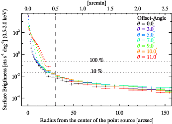
Figure 1: Shape of the PSF for Chandra ACIS-I (averaged over 4 azimuthal angles) for different offset angles ($\theta$) for the source flux of $0.63\times 10^{-14}\,\mathrm{erg\,cm^{-2}\,s^{-1}\,deg^{-2}}$ ($0.5-2.0\,\mathrm{keV}$). The vertical dashed line shows the radius of the circular exclusion area for this flux group (Table 1). The horizontal dotted lines show levels corresponding to $100\,\%$ and $10\,\%$ of the surface brightness of unresolved AGN (Sect. 3.1.3).

2.1 Exposure map and mask

For the following data processing and analysis, we will need the exposure map $\mathbf{E}$ [seconds] and mask $\mathbf{M}$, which we describe here.

We use the exposure map $\mathbf{E}$ to convert our count maps $\mathbf{C}$ [counts] into flux maps $\mathbf{F}$ [cts s^-1] but also to take the vignetting into account. For creating the exposure map $\mathbf{E}$ we are using the spectral model and best-fit parameters of our spectral fit of the unresolved CXB (Table 2). Note that the exposure map $\mathbf{E}$ is not very sensitive to the choice of the spectral model in the $0.5-2.0\,\mathrm{keV}$ band, because we only compute the exposure map in units of seconds and the vignetting is not very energy depended in this energy range.

We use the mask $\mathbf{M}$ to excluded certain regions of Chandra maps from the analysis. It is set to be large enough ($2900\times 2900$ pixels) to contain the entire ACIS-I FOV of an observation. Pixels of the mask are set to zero, when they are outside the FOV, when they are within the exclusion area of a resolved source (Sect. 2.2), when they have zero exposure time, which takes also bad pixels into account, or when the exposure time falls below $63\,\%$ of the peak value of $\mathbf{E}$. The latter targets low exposed pixels, which are predominantly located in the CCD gaps and edges of the ACIS-I and occur due to the dithering movement of Chandra during an observation. The threshold was chosen to be $63\,\%$, because we see a clear break of the pixel distribution of $\mathbf{E}$ around this value. The average field-of-view (FOV) solid angle of one observation after this filter step but before removing resolved sources is $\sim 0.07\,\mathrm{deg^{2}}$. The solid angle of the mask is computed as

$$\Omega=(\Delta p)^{2}\,\left(\Sigma_{i,j}M_{i,j}\right)\text{ ,}$$ (1)

whereby $\Delta p$ is the size of a pixel. Since for our analysis we use an image pixel binning of one, the size of a pixel is $\Delta p=0.492\arcsec$.

Whenever we convert counts to count-rate, where we can not use the exposure map $\mathbf{E}$, we are using the average value of this map:

$$\langle E\rangle=\dfrac{\Sigma_{i,j}E_{i,j}\,M_{i,j}}{\Sigma_{i,j}M_{i,j}}\text{ ,}$$ (2)

This for instance is the case for the energy spectrum in Sect. 3 or for energy bands above $9\,\mathrm{keV}$, where the effective area of Chandra becomes neglectable.

2.2 Removing resolved sources

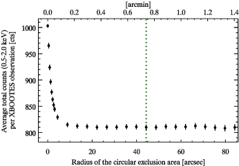
Figure 2: Average total counts ($0.5-2.0\,\mathrm{keV}$) per XBOOTES observation (instrumental background not removed) as a function of radius of the circular exclusion area of point sources. We change the radius for each flux group between $1\,\%$ to $200\,\%$ of its value in Table 1. The displayed radius is a weighted average based on the number of point sources per flux group. Vertical dotted line: Average radius for our definition in Table 1.

Table 1: Radius of the circular exclusion area of resolved point sources in XBOOTES for different flux groups.

Flux	# of	(b)	Radius	Depth(c)	ECF(d)	(e)
Groups(a)	Sources	[%]	[arcsec]	[%]	[%]	[cts]
$[0.47,0.63[$	1673	$\sim 51$	30	$\sim 10$	$\sim 98.4$	$\sim 0.06$
$[0.63,2.10[$	1328	$\sim 40$	55	$\sim 10$	$\sim 98.7$	$\sim 0.16$
$[2.10,9.00[$	268	$\sim 8$	80	$\sim 25$	$\sim 99.0$	$\sim 0.55$
$[9.0,47.0[$	23	$\sim 1$	140	$\sim 50$	$\sim 99.4$	$\sim 1.76$

(a) In $10^{-14}$ erg cm^-2 s^-1 ($0.5-2.0\,\mathrm{keV}$).

(b) Number of sources in fraction of the total number of sources (3293).

(c) The PSF surface brightness in fraction of the surface brightness of unresolved AGN (Sect. 3.1.3) for the brightest sources in the given flux group at the edge of the circular exclusion area.

(d) Enclosed count fraction (based on the integration of our simulated PSF, averaged over all azimuthal and offset angles).

(e) Residual counts per point-source outside the exclusion area for the brightest sources in the given flux group. Computed with the corresponding ECF and an exposure time of $4.3$ ksec (average value for XBOOTES, Sect. 2.3).

In order to study the unresolved CXB, we need to remove the resolved (point-like and extended) sources to such a level that the residual counts of resolved sources contribute only insignificantly to the surface brightness of the unresolved CXB. For this purpose we are using the two source catalogs of K05 for point and extended sources.

2.2.1 Point sources

The point-source catalog of K05 includes 3293 sources with at least 4 counts in the $0.5-7.0\,\mathrm{keV}$ band. The sky coverage of the XBOOTES survey as a function of the point-source detection sensitivity is shown in Fig. 12 of K05 (for the $0.5-7.0\,\mathrm{keV}$ band). The average flux limit of the survey in the $0.5-2.0\,\mathrm{keV}$ band is $\sim 2.3\times 10^{-15}\,\mathrm{erg\,cm^{-2}\,s^{-1}}$. It is defined as the flux level, which gives the same resolved CXB fraction as computed with the sky coverage vs. sensitivity distribution of the survey (e.g.  Eq. 9). To estimate the appropriate size of a circular exclusion area of a point source, we simulated the point-spread-function (PSF) shape for 13 offset angles ($\theta=0\arcmin-12\arcmin$, in $1\arcmin$-steps) and for four equally distributed azimuthal angles (from the aimpoint roughly along the diagonal of each CCD) with the Chandra Ray Tracer simulator (Carter et al., 2003) and the MARX software package (v5.0.0), as shown in Fig. 1 for the average over all azimuthal angles. Based on these simulations we define the circular exclusion area as presented in Table 1, where we split the point sources into different flux groups in order to make source removal more efficient. The shape of the PSF does not depend on the flux of a point source but the normalization of the PSF does. Hence, for each flux group the PSF normalization is defined by the upper-limit of its flux-interval (first column of Table 1). For the first two flux groups, which represent about $90\,\%$ of all point sources, the radius of the exclusion area is chosen in the way that both groups are removed at a same depth. We quantify this depth with the surface brightness of the PSF at the edge of the exclusion area, which corresponds for both groups to $\sim 10\,\%$ of the surface brightness of unresolved AGN (Sect. 3.1.3). For the other two flux groups we make a compromise in the depth in order to keep the radius of the exclusion area in a reasonable regime. In our simulations we further find that for radii of $\gtrsim 20\arcsec$ the PSF shape does not change very significantly as a function of azimuthal and offset angle (Fig. 1). Therefore, we use in the following a PSF averaged over all four azimuthal angles and all offset angles. With this we compute the enclosed count fraction (ECF) and residual counts of a point source for each flux-group, which are displayed as well in Table 1.

In order to test that our definition of the exclusion area of point sources in Table 1 removes sufficiently well the counts of resolved sources, we estimated how the average total counts per XBOOTES observation change as a function of radius of the exclusion area (Fig. 2). We create a list of evaluation steps, where we set the radius from $1\,\%$ to $200\,\%$ of its value in Table 1 in each flux group. For presentation purposes (Fig. 2), we compute an average radius per evaluation step of all flux groups, where we weight the radius of each flux group by the corresponding number of point sources. The measured number of total counts per observation is normalized for each evaluation step to the surface area of the observation before sources were removed. To ensure a clean test without any bias due to our choice of removing the extended sources (Sect. 2.2.2), we take here only those observations into account (83 out of 118 observations), which do not contain extended sources.

The result of this test is shown in Fig. 2. We can see for radii of $\gtrsim 20\arcsec$ that the total counts do not change significantly. The rise in total counts for $\lesssim 20\arcsec$ indicates that there is still a significant contamination by counts from resolved point sources at these apertures. The average radius of our definition of the exclusion area in Table 1 is $\approx 44\arcsec$ (weighted with number of point sources per flux group) and is shown as vertical dotted line in Fig. 2. This figure demonstrates that our definition of the exclusion regions for point sources is rather conservative. In average the FOV is reduce by $\sim 17\,\%$ after removing all resolved point sources with our definition.

To estimate contamination by the residual source counts, we note the following. With our definition of the point-source exclusion area, the ECF averaged over all resolved point sources equals to $\sim 98.6\,\%$, i.e. about $\approx 1.4\%$ of the point source counts in the wings of the PSF remain in the image. Using observations without resolved extended sources (83 of 118) we compute the average number of counts in the exclusion regions, $\approx 181$ counts per observation in the $0.5-2.0\,\mathrm{keV}$ band. Therefore, there is about $\approx 2.6$ residual counts per image left from the resolved point sources. This should be compared with the total number of counts in the unresolved emission, $\approx 601$ per image, of which $\approx 208$ are from unresolved CXB and $\approx 393$ are due to the instrumental background. Thus, residual counts from resolved point sources constitute about $\approx 1\%$ of the total unresolved CXB counts, i.e. their contamination can be neglected.

2.2.2 Extended sources

There are 43 extended sources detected with a detection limit of $\approx 1\times 10^{-14}\,\mathrm{erg\,cm^{-2}\,s^{-1}}$ ($0.5-2.0\,\mathrm{keV}$) (K05, Sect. 3.2. & Table 1). The extended sources in the XBOOTES catalog were fitted with a Gaussian model in order to estimate their size. We define the radius of the circular exclusion area as six times this size. We tested circular exclusion areas between four and eight times the size and did not find any significant difference in the remaining source counts after we normalize to the same surface area. Therefore, we believe that this is a reasonable definition. We also note that the total source counts of the resolved extended sources only accounts $\sim 4\,\%$ to the total source counts of all resolved sources, based on the source catalogs of XBOOTES.

2.2.3 Summary

After removing all resolved sources the average FOV area is reduced by $\sim 18\%$ down to $\sim 0.0610\,\mathrm{deg^{2}}$. The average surface brightness is reduced by $\sim 43\%$ from $1.42\pm 0.01$ to $0.81\pm 0.01\,\mathrm{cts\,s^{-1}deg^{-2}}$ in the $0.5-2.0\,\mathrm{keV}$ band (after removing the instrumental background, see Sect. 2.3 and 2.4).

2.3 Removing background flares

In order to detect and remove time intervals of an observation, which are contaminated by background flares, we adopt the main concept of Hickox & Markevitch (2006, hereafter H06) and adjust them to the XBOOTES data. We analyze the light curve of each observation in the energy-band $2.3-7.3\,\mathrm{keV}$. H06 show that this band is the best choice for background flare detection, because of the different energy-spectra of background flares and the quiescent background (see their Fig. 3).

Our de-flaring method consists of three consecutive steps of filtering the light curve:

(a) We run a $3\sigma$-clipping with the CIAO tool deflare, which is a standard procedure and removes the most obvious flares. Hereby, we use bins of $\sim 63$ sec (10 frames), which is large enough to assume a Gaussian error distribution in each time bin but small enough to not conceal short, strong flares.

(b) We create a light curve with a binning of $\sim 252$ sec (80 frames) and remove all bins, which are $30\,\%$ above the mean count rate of the $3\sigma$-clipped light curve from step (a). This step targets weaker and longer lasting flares with a maximum duration of the order of the bin size. In comparison to H06, we only remove positive deviations from the mean.

(c) We compute a light curve in bins of $\sim 252$ sec (80 frames) of the ratio between the $2.3-7.3\,\mathrm{keV}$ and $9.5-12.0\,\mathrm{keV}$ band and remove all bins, which are $40\,\%$ above the mean ratio of all considered XBOOTES observations. This method was introduced by H06 and is best suited for weak flares. It takes advantage of the fact that for a typical flare the flux-ratio of $2.3-7.3\,\mathrm{keV}$ to $9.5-12.0\,\mathrm{keV}$ band will be larger than for the normal instrumental background (alias quiescent background) due to the different energy-spectrum shapes. We use the same threshold for all observations to ensure a constant energy-spectrum shape for all of them.

The major difference between H06 and our filtering arises due to the fact that our observations have exposure times of the order of kiloseconds, whereas H06 use observations with more than one Megasecond. This leads in our case to much smaller bin sizes for the light curves and less restrictive thresholds for removing flare events for step (b) and (c). The light curves of all observations were visually inspected and the thresholds of (b) and (c) were tuned to removed any obvious feature of the light curve, which could be interpret as a background flare.

For a typical observation, our de-flaring method removes on average $\sim 190$ sec ($\sim 4\,\%$) of the exposure time. After the de-flaring we have an average exposure time per observation of $\sim 4.3$ ksec and a total exposure time is reduced to $\sim 0.50$ Msec. We note that de-flaring does not significantly affect the power spectrum of the unresolved CXB, but it is necessary for accurate measurement of the absolute CXB flux (Sect. 3).

2.4 Instrumental background and background-subtracted map

We estimate the contribution of the instrumental background with the method presented in H06. They show in their study with the Chandra’s ACIS-I stowed background data that the shape of the energy spectrum of the instrumental background of ACIS-I from different observations is very stable over the course of five years, which includes the time when the XBOOTES observations were performed. Further, we know that all detected photons in the $9.5-12.0\,\mathrm{keV}$ band are due to the instrumental background because the effective area of Chandra in this energy range is neglectable. With those two facts combined we can estimate the instrumental-background map $\mathbf{C}^{\mathrm{BKG}}$ for an observation with the total-count map $\mathbf{C}^{\mathrm{Total}}$ in the energy band $X$ by scaling the ACIS-I stowed-background map $\mathbf{C}^{\mathrm{Stow}}$ as following:

$$\mathbf{C}_{X}^{\mathrm{BKG}}=\mathbf{M}\cdot\mathbf{C}_{X}^{\mathrm{Stow}}\cdot\left(\dfrac{\Sigma_{i,j}\,C_{9.5-12.0\,\mathrm{keV}}^{\mathrm{Total}}\,M}{\Sigma_{i,j}\,C_{9.5-12.0\,\mathrm{keV}}^{\mathrm{Stow}}\,M}\right)\text{ .}$$ (3)

With this method we estimate an average background surface brightness of $1.55\pm 0.01\,\mathrm{cts\,s^{-1}deg^{-2}}$ in the $0.5-2.0\,\mathrm{keV}$ band, which is consistent with the value from the spectral fit (see also Table 6). This means that $\sim 65\,\%$ of the total surface brightness of $2.37\pm 0.01\,\mathrm{cts\,s^{-1}deg^{-2}}$ (after removing resolved sources, Sect. 2.2) is due to the instrumental background.

The background-subtracted map is then

$$\mathbf{C}_{X}^{\mathrm{CXB}}=\mathbf{C}_{X}^{\mathrm{Total}}\,\mathbf{M}-\mathbf{C}_{X}^{\mathrm{BKG}}\text{ .}$$ (4)

We estimate from the background-subtracted map (after removing resolved sources) the average surface brightness of the the unresolved CXB equal to $0.81\pm 0.01\,\mathrm{cts\,s^{-1}deg^{-2}}$, which in physical units corresponds to $7.9\pm 0.1\,\times 10^{-12}\,\mathrm{erg\,cm^{-2}\,s^{-1}\,deg^{-2}}$, using our spectral model of the unresolved CXB from Sect. 3. This value is consistent with $7.8\pm 0.1\,\times 10^{-12}\,\mathrm{erg\,cm^{-2}\,s^{-1}\,deg^{-2}}$ obtained from the spectral fit in Sect. 3.1.1.

We show in App. D.2 that in the $0.5-2.0\,\mathrm{keV}$ band, surface brightness fluctuations of the instrumental background are much smaller than fluctuations of unresolved CXB. Therefore subtraction of the instrumental background is unnecessary for the calculation of the power spectrum of CXB fluctuations. Accordingly, it is not performed in Sect. 4 where total-count maps ($\mathbf{C}^{\mathrm{Total}}$) are used for construction of the power spectra. However, accurate account for the instrumental background is necessary for computing the CXB flux and its spectral analysis.

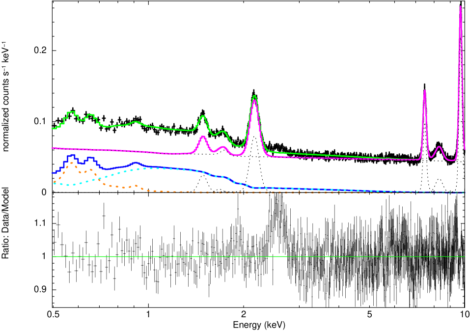
Figure 3: The 0.5–10 keV stacked energy spectrum of 118 XBOOTES observations after removing resolved sources (black crosses, Sect. 2.2). Note that for our brightness fluctuation analysis in Sect. 4 we only use the $0.5-2.0\,\mathrm{keV}$ band. The lower panel shows the ratio of model and data. Green solid curve: Total model (CXB and background model). Dark blue solid curve: Total CXB model (Table 2). Light blue dotted curve: absorbed powerlaw model (phabs(powerlaw)), representing the contribution of extragalactic emission. Orange dotted curve: APEC, representing the contribution of Galactic emission. Pink solid curve: Instrumental background model (App. A). Black dotted curves: components of the instrumental background model.

2.5 Flux and fluctuation maps

The flux map $\mathbf{F}_{X}$ of the energy band $X$ is computed as the ratio between the count and exposure map (for each pixel):

$$\mathbf{F}_{X}=\mathbf{M}\cdot\dfrac{\mathbf{C}_{X}}{\mathbf{E}}\text{ ,}$$ (5)

and is only computed in instrumental units [cts s^-1]. The average flux map $\langle\mathbf{F}\rangle$ is defined as:

$$\langle\mathbf{F}_{X}\rangle=\mathbf{M}\cdot\left(\dfrac{\Sigma_{i,j}\,C_{X}\,M}{\Sigma_{i,j}\,E\,M}\right)\text{ .}$$ (6)

These definitions minimizes statistical errors, while taking the vignetting of the exposure map properly into account. Note, that in order to compute the average count map $\langle\mathbf{C}\rangle$, which also treats vignetting properly, one has to multiply $\langle\mathbf{F}\rangle$ with the exposure map:

$$\langle\mathbf{C}_{X}\rangle=\langle\mathbf{F}_{X}\rangle\cdot\mathbf{E}\text{ .}$$ (7)

For our analysis in Sect. 4 we need the fluctuation map $\delta\mathbf{F}$ in different energy bands for each observation. We compute this map for an energy band $X$ as following:

$$\delta\mathbf{F}_{X}=\mathbf{F}_{X}-\left\langle\mathbf{F}_{X}\right\rangle\text{ .}$$ (8)

3 Composition of the unresolved CXB

3.1 Energy spectrum

The unresolved CXB consists of two components: the Galactic and extragalactic emission. We will use spectral analysis to separate their contributions to the CXB. We create the energy spectrum by stacking the energy spectra of all 118 considered XBOOTES observations, after removing resolved sources (Sect. 2.2) and background flares (Sect. 2.3). The stacked energy spectrum has a total exposure time of $\sim 0.50$ Msec and is based on a total surface area of $\sim 7.2\,\mathrm{deg^{2}}$ (without taking overlaps into account). We fit it in the energy range of $0.5-10.0\,\mathrm{keV}$ with a model for the unresolved CXB (Sect. 3.1.1, blue curve in Fig. 3) and an instrumental background model (App. A, pink curve in Fig. 3).

3.1.1 Spectral model

Table 2: Best-fit parameters of our spectral model (APEC + phabs(powerlaw), Sect. 3.1.1) of the unresolved CXB of XBOOTES (Fig. 3).

Model Component	Parameter	Value
APEC	Temperature ($T$)	$0.164\pm 0.003\;\mathrm{keV}$
	Normalization	$1.9\pm 0.1\;\times 10^{-4}\;\mathrm{cm^{-5}}$
	Surface Brightness(a)	$3.2\pm 0.1\;\times 10^{-12}$
phabs(powerlaw)	$N_{\mathrm{H}}$ (fixed)	$10^{20}\;\mathrm{cm^{-2}}$
	Photon Index ($\Gamma$)	$1.74\pm 0.03$
	Normalization(b)	$1.23\pm 0.02\;\times 10^{-4}$
	Surface Brightness(a)	$4.6\pm 0.1\;\times 10^{-12}$

(a) $\mathrm{erg\,cm^{-2}\,s^{-1}\,deg^{-2}}$ ($0.5-2.0\,\mathrm{keV}$); (b) $\mathrm{photons\,keV^{-1}\,cm^{-2}\,s^{-1}}$ at $1\;\mathrm{keV}$.

Our spectral model for the unresolved CXB consists of an absorbed powerlaw (phabs(powerlaw)) with a fixed absorption column of $N_{\mathrm{H}}=10^{20}\mathrm{cm^{-2}}$ (Kalberla et al., 2005, K05) and of an unabsorbed APEC model, the former representing the extragalactic sources and the latter representing the Galactic diffuse emission. The spectrum and model fit are shown in Fig. 3 and the best-fit parameters are listed in Table 2. The CXB model gives a surface brightness of $7.8\pm 0.1\,\times 10^{-12}\,\mathrm{erg\,cm^{-2}\,s^{-1}\,deg^{-2}}$ ($0.81\pm 0.01\,\mathrm{cts\,s^{-1}deg^{-2}}$) in the $0.5-2.0\,\mathrm{keV}$ band, which is in good agreement with the value from the flux maps of $7.9\pm 0.1\,\times 10^{-12}\,\mathrm{erg\,cm^{-2}\,s^{-1}\,deg^{-2}}$ (Sect. 2.4). The individual components of our CXB model are discussed in the following sections.

We note that there is a significant emission feature in the energy spectrum around $2.5\,\mathrm{keV}$ (close to the right wing of the third instrumental line, Fig. 3). We believe that it arises from the instrumental background, since we can see a similar feature in the spectrum of the latter (Fig. 14). This is further supported by the fact that we do not detect any excess continuum associated with this feature. However, we can not entirely exclude the possibility that it may be of astrophysical origin As it is outside the energy range of our fluctuation analysis ($0.5-2.0\,\mathrm{keV}$) we do not investigate it any further here.

3.1.2 Galactic emission

The APEC model of our spectral model encapsulates all the Galactic emission, which is a superposition of various diffuse sources (e.g. Lumb et al., 2002; Hickox & Markevitch, 2006; Henley & Shelton, 2013): the Galactic halo emission and the foreground emission, which is a composite of emission from solar wind charge exchange (SWCX) and the local bubble. All of them have in common that they are anisotropically distributed over the sky. In Fig. 3 we can see that the Galactic emission dominates the soft part of the energy spectrum but above $\sim 1\,\mathrm{keV}$ it becomes negligibly small in comparison to the extragalactic component.

The surface brightness of our Galactic emission model is $3.2\pm 0.1\,\times 10^{-12}$ erg cm^-2 s^-1 deg^-2 for the $0.5-2.0\,\mathrm{keV}$ band (Table 2). This is in reasonable agreement with the measurements of H06 (Table 2, $\sim(3-4)\times 10^{-12}\,\mathrm{erg\,cm^{-2}\,s^{-1}\,deg^{-2}}$), which use Chandra Deep Field surveys (hereafter CDFs), and Lumb et al. (2002, Table 3, $\sim 3.8\times 10^{-12}\,\mathrm{erg\,cm^{-2}\,s^{-1}\,deg^{-2}}$), which use several deep XMM-Newton observations.

3.1.3 Extragalactic emission

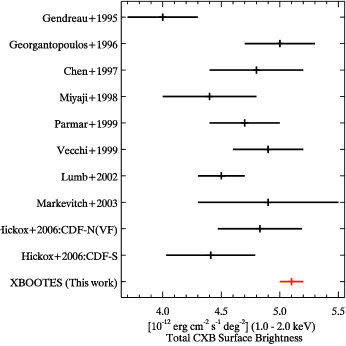
Figure 4: Comparison of recent surface brightness measurements of the CXB in the $1.0-2.0\,\mathrm{keV}$ band. See also Table 5 and Table 6 (last column) of H06.

The absorbed powerlaw (phabs(powerlaw)) of our spectral model describes the extragalactic emission and its total surface brightness is $4.6\pm 0.1\,\times 10^{-12}\,\mathrm{erg\,cm^{-2}\,s^{-1}\,deg^{-2}}$ for the $0.5-2.0\,\mathrm{keV}$ band. Together with the emission of the resolved sources ($4.4\pm 0.1\,\times 10^{-12}\,\mathrm{erg\,cm^{-2}\,s^{-1}\,deg^{-2}}$) computed from the removed source counts and converted to physical units with the same spectral model, we obtain for XBOOTES a total extragalactic CXB surface brightness of $9.0\pm 0.1\,\times 10^{-12}\,\mathrm{erg\,cm^{-2}\,s^{-1}\,deg^{-2}}$. The values are summarized in Table 3.

We can see in Fig. 3 that the extragalactic emission dominates the energy spectrum above $\sim 1\,\mathrm{keV}$. For the $1.0-2.0\,\mathrm{keV}$ band it has a surface brightness of $2.6\pm 0.1\,\times 10^{-12}\,\mathrm{erg\,cm^{-2}\,s^{-1}\,deg^{-2}}$, while the Galactic emission has less than $0.1\times 10^{-12}\,\mathrm{erg\,cm^{-2}\,s^{-1}\,deg^{-2}}$, based on our spectral model. Therefore, the contribution by any known Galactic sources can be neglected, which makes the $1.0-2.0\,\mathrm{keV}$ band very suitable to compare our extragalactic CXB measurement with other studies. In Fig. 4 we show a summary of previous CXB measurement taken from H06 (Table 5 and Table 6, last column) together with our measurement. A comparison reveals that our measurement is the highest but still in good agreement with almost all of these studies. Except for the measurement of Gendreau et al. (1995) with ASCA, the differences remains below $14\,\%$. We are consistent within one standard deviation with the CDF-North (CDF-N) ($4.8\pm 0.4\,\times 10^{-12}\,\mathrm{erg\,cm^{-2}\,s^{-1}\,deg^{-2}}$) and within two standard deviation with the CDF-South (CDF-S) ($4.4\pm 0.4\,\times 10^{-12}\,\mathrm{erg\,cm^{-2}\,s^{-1}\,deg^{-2}}$). Note that since both CDFs are deep pencil-beam surveys with a sky area of $\sim 0.02$ deg² each, which is about $400$ times smaller than for XBOOTES, cosmic variance needs to be considered. H06 estimate that this adds an additional uncertainty of about $\sim(10-20)\,\%$ to the measurement of the CDFs. Furthermore, the much bigger sky area used in our analysis (by a factor of $\sim 100$) is the main reason of our much smaller statistical uncertainty in comparison to the CDFs.

Table 3: Extragalactic emission of XBOOTES
[$10^{-12}\,\mathrm{erg\,cm^{-2}\,s^{-1}\,deg^{-2}}$].

	$0.5-2.0\,\mathrm{keV}$	$1.0-2.0\,\mathrm{keV}$
Unresolved(a)	$4.6\pm 0.1$	$2.58\pm 0.05$
Resolved(b)	$4.4\pm 0.1$	$2.48\pm 0.03$
Total	$9.0\pm 0.1$	$5.1\pm 0.1$

(a) From the spectral fit (Table 2); (b) From the removed source counts of the resolved sources in the background-subtracted maps (Sect. 2.2-2.4).

3.2 Flux budget

The unresolved extragalactic emission is a superposition of contributions of various types of sources of which most important are expected to be: AGN, normal galaxies (no indication of AGN activity), and clusters and groups of galaxies, which we refer to in the following as the major X-ray source populations (e.g. Lumb et al., 2002; De Luca & Molendi, 2004; Hickox & Markevitch, 2006, 2007; Kim et al., 2007; Georgakakis et al., 2008; Lehmer et al., 2012; Rosati, Borgani & Norman, 2002; Finoguenov et al., 2007, 2010, 2015). Here, we estimate the absolute and fractional contribution of each population to the unresolved extragalactic emission, which will be relevant for our fluctuation analysis (Sect. 4 and 5). We compute the surface brightness of the unresolved emission of an X-ray population as follows:

$$B =\int\limits_{S_{\mathrm{Min}}}\mathrm{d}S\;S\,\frac{\mathrm{d}N}{\mathrm{d}S}\;\left(1-f(S)\right)\text{ .}$$ (9)

Hereby, we use differential $\log N-\log S$ from the literature and the normalized XBOOTES survey sensitivity curve $f(S)$ for each source population.

Lehmer et al. (2012, hereafter L12) present the currently best measurement of the $\log N-\log S$ of AGN and normal galaxies, which is based on source samples down to a flux limit of $S_{0.5-2.0\,\mathrm{keV}}\sim 10^{-17}\,\mathrm{erg\,cm^{-2}\,s^{-1}}$. They demonstrated that above this flux limit AGN dominate the source counts, while below it normal galaxies are becoming the dominant source population (see Fig. 6 of L12). We find a very good agreement between the $\log N-\log S$ of L12 and of XBOOTES (K05) down to the flux-limit of XBOOTES ($\sim 2\times 10^{-15}\,\mathrm{erg\,cm^{-2}\,s^{-1}}$). Based on the $\log N-\log S$ of L12, we estimate a surface brightness of $B_{\mathrm{AGN}}\sim 1.4\times 10^{-12}\,\mathrm{erg\,cm^{-2}\,s^{-1}\,deg^{-2}}$ and $B_{\mathrm{Nor.Gal.}}\sim 2.2\times 10^{-13}\,\mathrm{erg\,cm^{-2}\,s^{-1}\,deg^{-2}}$ for the unresolved AGN and normal galaxy population in XBOOTES, respectively. For this we used the Eq. (9), the point-source sensitivity distribution of XBOOTES (Fig. 12 of K05, see also Sect. 2.2), and a flux limit of L12 of $S_{\mathrm{Min}}=10^{-17}\,\mathrm{erg\,cm^{-2}\,s^{-1}}$. If we extrapolate the $\log N-\log S$ of L12 by two orders of magnitude down to $S_{\mathrm{Min}}=10^{-19}\,\mathrm{erg\,cm^{-2}\,s^{-1}}$, the surface brightness of AGN increases by $\sim 6\,\%$ ($B_{\mathrm{AGN}}\sim 1.5\times 10^{-12}\,\mathrm{erg\,cm^{-2}\,s^{-1}\,deg^{-2}}$) and of normal galaxies by a factor of $\sim 3.5$ ($B_{\mathrm{Nor.Gal.}}\sim 7.8\times 10^{-13}\,\mathrm{erg\,cm^{-2}\,s^{-1}\,deg^{-2}}$).

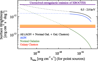
Figure 5: The predicted surface brightnesses of unresolved X-ray source populations in XBOOTES ($0.5-2.0\,\mathrm{keV}$) as a function of the lower flux limit $S_{\mathrm{Min}}$ of Eq. (9) for point sources. The dotted part of a curve illustrates, where we extrapolate the used $\log N-\log S$. Note that these parts of the curves should be interpreted with some caution as they represent extrapolations over several orders of magnitude. The orange bar shows the contribution by clusters and groups of galaxies. The lower limit of the bar (red line) illustrates the default estimate of Table 4, while for the upper limit the XLF slope of Ebeling et al. (1997) is increased by $\sim 10\,\%$. Purple horizontal line: The unresolved extragalactic emission of XBOOTES (Table 3). The thickness of the line represents one standard deviation.

This calculation shows that the total flux of AGN is relatively independent of $S_{\mathrm{Min}}$, while for normal galaxies it is very sensitive to $S_{\mathrm{Min}}$, as it is further illustrated in Fig. 5. Such a behavior is caused by the steeper slope of the $\log N-\log S$ of normal galaxies in comparison to AGN ($\beta\approx 2.2$ for normal galaxies, $\beta\approx 1.5$ for AGN) and makes it difficult to estimate accurately the contribution of normal galaxies to the unresolved CXB emission.

Table 4: Contributions of major X-ray source populations to the unresolved extragalactic emission of XBOOTES.

Contribution	Absolute(a)		Fractional(b)
Energy-Band(c) [keV]	$0.5-2.0$	$1.0-2.0$	$0.5-2.0$
AGN(d)	$\sim 1.51$	$\sim 0.85$	$\sim 33\,\%$
Normal Galaxies(d)	$\sim 1.35$	$\sim 0.76$	$\sim 29\,\%$
Galaxy Clusters(e)	$\sim 0.25$	$\sim 0.15$	$\sim 6\,\%$
Sum	$\sim 3.11$	$\sim 1.77$	$\sim 68\,\%$

(a) In units of $10^{-12}\,\mathrm{erg\,cm^{-2}\,s^{-1}\,deg^{-2}}$. (b) In respect to the unresolved extragalactic emission of XBOOTES (Table 3). (c) Spectral models for energy band conversion are described in Sect. 5.4.3. (d) Lower flux limit: $S_{\mathrm{Min}}=10^{-20}\,\mathrm{erg\,cm^{-2}\,s^{-1}}$ ($0.5-2.0\,\mathrm{keV}$). (e) Lower temperature limit: $T=0.2\,\mathrm{keV}$ ($L_{\mathrm{0.5-2.0\,\mathrm{keV}}}\gtrsim 10^{40.2}\,\mathrm{erg\,s^{-1}}$, $M_{500}\gtrsim 10^{12.8}\,\mathrm{M_{\sun}\,h^{-1}}$ for $z=0$).

To estimate the contribution of clusters and groups of galaxies to the unresolved emission of XBOOTES, we are using the X-ray luminosity function (XLF) of Ebeling et al. (1997). It is based on the ROSAT Brightest Cluster sample (BCS, Ebeling et al., 1996), which includes 199 sources with a flux above $\sim 5\times 10^{-12}\,\mathrm{erg\,cm^{-2}\,s^{-1}}$, and covers redshifts up to $z\sim 0.3$ and luminosities down to $5\times\sim 10^{42}\,\mathrm{erg\;s^{-1}}$ ($0.1-2.4\,\mathrm{keV}$). Despite the small redshift range of the XLF, it predicts consistent number densities of galaxy clusters down to the currently deepest studies with XMM-Newton having the sensitivity limit for extended sources of $S_{0.5-2.0\,\mathrm{keV}}\sim 10^{-16}\,\mathrm{erg\,cm^{-2}\,s^{-1}}$ (e.g. Rosati, Borgani & Norman, 2002; Finoguenov et al., 2007, 2010, 2015). Further, the XLF does not incorporate any redshift evolution, which is consistent with more recent studies over a larger redshift range up to $z\sim 1$ (e.g. Böhringer, Chon & Collins, 2014; Pacaud et al., 2016). To compute the $\log N-\log S$ from this XLF, we integrate the XLF over redshift and luminosity. For the K-correction in this integration, we are assuming an APEC model, where we couple its temperature to the luminosity with the luminosity-temperature scaling relation of Giles et al. (2015, Table 2, bold font) and assume a typical metallicity of $0.3$ of the solar value (Anders & Grevesse, 1989). As a lower temperature limit we use $T=0.2\,\mathrm{keV}$ ($\approx 2.3\times 10^{6}$ K). This limits our integration to luminosities above $\sim 10^{40.2}\,\mathrm{erg\,s^{-1}}$ ($0.5-2.0\,\mathrm{keV}$) and DMH masses above $M_{500}\sim 10^{12.8},\mathrm{M_{\sun}\,h^{-1}}$ ($z=0$), using the luminosity-mass relation of Anderson et al. (2015). It also leads to a decline of the differential $\log N-\log S$ at fluxes below $\sim 10^{-18}\,\mathrm{erg\,cm^{-2}\,s^{-1}}$.

We rescale the $\log N-\log S$ computed with XLF of Ebeling et al. (1997) by a factor of $0.60$ to match the observed $\log N-\log S$ of extended sources in XBOOTES (K05, Table 1). We note that the scaled $\log N-\log S$ is still consistent within one standard deviation with the measurements of Finoguenov et al. (2010, 2015). Based on the shape comparison of the $\log N-\log S$ of Ebeling et al. (1997) and the XBOOTES (K05, Table 1), we estimate that the sensitivity limit for extended sources for XBOOTES is around $S_{0.5-2.0\,\mathrm{keV}}=3\times 10^{-14}\,\mathrm{erg\,cm^{-2}\,s^{-1}}$. With this we estimate a surface brightness of $\sim 2.5\times 10^{-13}\,\mathrm{erg\,cm^{-2}\,s^{-1}\,deg^{-2}}$ for the unresolved clusters and groups of galaxies in XBOOTES.

The computed surface brightness of unresolved clusters and groups of galaxies depends only mildly on the assumed flux limit of XBOOTES for extended sources. For instance, the surface brightness only changes by $\sim 10\,\%$, if we change the flux limit by $-30\,\%$ or $+50\,\%$ ($(2.1-4.5)\times 10^{-14}\,\mathrm{erg\,cm^{-2}\,s^{-1}}$). Also the exact choice of the lower temperature limit in the XLF integration is not very critical. The surface brightness increases only by $\sim 2\,\%$, if we decrease the limit to $T=0.1\,\mathrm{keV}$ ($-50\,\%$) and it decreases only by $\sim 10\,\%$, if we increase the limit to $T=0.3\,\mathrm{keV}$ ($+50\,\%$). However, the estimate of the surface brightness of clusters and groups of galaxies is rather sensitive to the assumed shape of their XLF. For example, increasing its slope by $\sim 10\,\%$, from $\alpha=1.85$ to $2.03$, would increase the flux from unresolved clusters and groups of galaxies by $\sim 50\,\%$. This makes the estimate of their contribution to the unresolved part of the CXB less certain than that of AGN (but still more accurate than the estimate for normal galaxies).

The total flux budget for the unresolved CXB is summarised in Table 4. In computing these numbers we assumed the low flux limit for the $\log N-\log S$ integration of AGN and normal galaxies to be equal to $S_{\mathrm{Min}}=10^{-20}\,\mathrm{erg\,cm^{-2}\,s^{-1}}$ (note that as the contribution of clusters and groups of galaxies is computed via their XLF, no explicit low flux limit is needed in this case). With this AGN account for $\sim 33\,\%$ of the unresolved CXB in XBOOTES, normal galaxies for $\sim 29\,\%$ and clusters and groups of galaxies for $\approx 6\,\%$. All together they account for $\approx 68\,\%$ of the unresolved CXB. About $\approx 32\,\%$ of the unresolved emission remains unaccounted for in this calculation. This is not worrisome however, because of the rather large uncertainty for the contribution of clusters and groups of galaxies and normal galaxies.

We illustrate the dependence of the surface brightness of unresolved AGN and normal galaxies on $S_{\mathrm{Min}}$ in Fig. 5. As one can see, the contribution by normal galaxies strongly increases towards small $S_{\mathrm{Min}}$ and at $S_{\mathrm{Min}}\sim 10^{-21}\,\mathrm{erg\,cm^{-2}\,s^{-1}}$ can easily explain the remaining part of the unresolved CXB. Although this conclusion is based on a very significant extrapolation of the observed $\log N-\log S$ and should be interpreted with caution, it is clear that normal galaxies are an important contributor to the unresolved CXB in XBOOTES. This inference is further supported by the results of Hickox & Markevitch (2007) who showed that faint optical/IR point sources can be associated with $\sim 50\,\%$ of the extragalactic emission below $S_{0.5-2.0\,\mathrm{keV}}\sim 10^{-17}\,\mathrm{erg\,cm^{-2}\,s^{-1}}$. Combining this result with the $\log N-\log S$ of resolved normal galaxies at higher fluxes, we estimate that normal galaxies account for at least $\sim 34\,\%$ of the unresolved extragalactic CXB in XBOOTES, which is close to the value derived above (Table 4).

3.3 Redshift and luminosity distributions of unresolved populations

Figure 6: Flux production rate in the $0.5-2.0\,\mathrm{keV}$ band for different populations in XBOOTES survey versus redshift and luminosity: unresolved AGN (left) and clusters and groups of galaxies (right). For the latter we show the flux production rate for both unresolved (solid curves) and total (dotted curve) populations. The vertical lines show corresponding median values.

In order to characterize the unresolved populations, we calculate their flux production rate per solid angle [erg cm^-2 s^-1 deg^-2] as a function of redshift and luminosity:

$$\ \frac{\mathrm{d}S(z)}{\mathrm{d}z}= \int\!\mathrm{d}S\;\left\{\dfrac{\Phi\!\left(\log_{10}(L_{r}[S,z]),z\right)}{L_{r}[S,z]\;\log_{\mathrm{e}}(10)}\right\}\;\frac{\mathrm{d}^{2}V(z)}{\mathrm{d}z\mathrm{d}\Omega}$$

$$\times\;\frac{4\pi d^{2}_{\mathrm{L}}(z)}{K(z)}\;S\;\left[1-f(S)\right]\text{,}$$ (10)

$$\frac{\mathrm{d}S(L)}{\mathrm{d}\log_{10}(L)}= \int\!\mathrm{d}z\;\Phi\!\left(\log_{10}(L_{r}),z\right)\;\frac{\mathrm{d}^{2}V(z)}{\mathrm{d}z\mathrm{d}\Omega}$$

$$\times\;S[L,z]\;\left[1-f(S[L,z])\right]\text{.}$$ (11)

where $\Phi(\log_{10}(L_{r}),z)$ [h³ Mpc^-3] is the luminosity function of sources, $f(S)$ is the normalized survey selection function of for the given type of objects (point-like or extended), $K(z)$ is the K-correction, $L_{r}$ [erg s^-1] is the rest-frame luminosity ($L_{r}=L/K(z)$), $\mathrm{d}^{2}V(z)/\mathrm{d}z/\mathrm{d}\Omega$ [Mpc³ h^-3 deg^-2] is the co-moving volume element, and $d_{\mathrm{L}}(z)$ [cm] is the luminosity distance (e.g. Hogg, 1999).

3.3.1 AGN

For the AGN luminosity function $\Phi(\log_{10}(L_{r}),z)$ [h³ Mpc^-3] we used results of Hasinger, Miyaji & Schmidt (2005) for the $0.5-2.0\,\mathrm{keV}$ band and for the $f(S)$ we use is the normalized survey selection function for point sources (K05, Fig. 12). For the XLF we include the exponential redshift cutoff for $z>2.7$: $\Phi(z)=\Phi(z\!=\!2.7)\times 10^{0.43\,(2.7-z)}$, which was proposed by Brusa et al. (2009). For computing the K-correction we assume a powerlaw with the photon-index of $\Gamma=1.7$, which simplifies the quantity to $K(z)=(1+z)^{2-\Gamma}$. The survey selection function is given in the $0.5-7.0\,\mathrm{keV}$ band and we convert it to the $0.5-2.0\,\mathrm{keV}$ band with an absorbed powerlaw with a photon-index of $\Gamma=1.7$. Note, that the XLF of Hasinger, Miyaji & Schmidt (2005) includes type 1 AGN only, and is defined for the minimum luminosity of $L_{0.5-2.0\,\mathrm{keV}}\approx 10^{42}\,\mathrm{erg\;s^{-1}}$ and maximum redshift of $z\approx 3-5$. Therefore we have to correct the amplitude of the differential flux distributions to match the $\log N-\log S$ of L12 (factor of $\sim 1.44$ increase). Secondly, one should be aware that the derived flux production rates may be subject to large uncertainties at low luminosity ($<10^{42}\,\mathrm{erg\;s^{-1}}$) and large redshift ($z>3$) (see also the discussion of the uncertainties of different XLF of AGN in Sect. 5 of Kolodzig et al., 2013b).

In Fig. 6 (left panels) we show the differential flux distributions of the unresolved AGN for the $0.5-2.0\,\mathrm{keV}$ band. The redshift distribution peaks around $z\sim 0.5$ with the median value of $z\sim 1.0$. About two thirds of unresolved AGN are located between redshift $\sim 0.4$ and $\sim 2.3$. The luminosity distribution peaks $\sim 10^{43.3}\,\mathrm{erg\;s^{-1}}$ and has the median value of $L\sim 10^{42.6}\,\mathrm{erg\;s^{-1}}$. About two thirds of unresolved AGN have the luminosity between $\sim 10^{41.0}$ and $\sim 10^{43.6}\,\mathrm{erg\;s^{-1}}$. Thus, that with the unresolved CXB of XBOOTES one can study the clustering signal of relatively low-luminosity AGN located around redshift $z\sim 1$. These objects are largely inaccessible for the conventional clustering studies using resolved AGN (e.g. Cappelluti, Allevato & Finoguenov, 2012; Krumpe, Miyaji & Coil, 2014).

3.3.2 Galaxy clusters & groups

As described in Sect. 3.2, for clusters and groups of galaxies we use the XLF of Ebeling et al. (1997), setting the lower integration limit corresponding to the gas temperature of $T=0.2\,\mathrm{keV}$ (Sect. 3.2). The selection function $f(S)$ is set to be a step-function with the step at the flux corresponding to the average survey sensitivity for extended source of $3\times 10^{-14}\,\mathrm{erg\,cm^{-2}\,s^{-1}}$ (Sect. 3.2). We also compute the flux production rate distributions for the entire population of clusters and groups of galaxies, as it will be relevant for the discussion in Sect. 5. In this case we assumed $f(S)=0$ for all fluxes. As with the AGN distributions, result of this calculation is subject to some uncertainty at low luminosities and large redshifts, where the XLF of the objects of interests is poorly constrained.

The obtained distributions are shown in Fig. 6. For the unresolved population, the redshift distribution has a median redshift of $z\sim 0.6$ and peaks around $z\sim 0.2$. The flux-weighted mean redshift equals $\left<z\right>\sim 0.3$. About two third of the population are located between redshift $\sim 0.2$ and $\sim 1.3$. Their median and peak luminosity is around $L\sim 10^{42.7}$ and $\sim 10^{43.1}\,\mathrm{erg\;s^{-1}}$, respectively, and about two third have a luminosity between $\sim 10^{41.4}$ and $\sim 10^{43.8}\,\mathrm{erg\;s^{-1}}$. Thus, the unresolved population of clusters and groups of galaxies consists mainly of relatively low-luminosity and nearby objects, located around redshift $z\sim 0.6$. They are more local and distributed over a more narrow redshift (and luminosity) range than unresolved AGN population.

The total (resolved and unresolved) population of clusters and groups of galaxies is located on average closer than its unresolved part, with a median redshift of $z\sim 0.4$ (peak at $z\sim 0.1$, flux-weighted mean of $\left<z\right>\sim 0.2$) and two third are located between redshift $\sim 0.1$ and $\sim 1.0$. The total population of clusters and groups of galaxies is in average more luminous than its unresolved part, with the median luminosity of $\sim 10^{43.4}\,\mathrm{erg\;s^{-1}}$ (peak at $\sim 10^{44.0}\,\mathrm{erg\;s^{-1}}$) and two thirds having the luminosity between $\sim 10^{42.0}$ and $\sim 10^{44.4}\,\mathrm{erg\;s^{-1}}$. Both results are expect since the resolved fraction of the total population consist of clusters and groups of galaxies, which contribute about $50\,\%$ to the total surface brightness of clusters and groups of galaxies and are rather close by and more luminous (Vajgel et al., 2014).

Based on the scaling relations at the median redshift and luminosity, we estimate that the unresolved and total population of clusters and groups of galaxies have in average an ICM temperature of $T\sim 1.4\,\mathrm{keV}$ ($\sim 1.6\times 10^{7}$ K) and $\sim 2.9\,\mathrm{keV}$ ($\sim 3.4\times 10^{7}$ K), and a DMH mass of $M_{500}\sim 10^{13.5}$ and $\sim 10^{14.0}\,\mathrm{M_{\sun}\,h^{-1}}$, respectively.

4 Brightness fluctuations of the unresolved CXB

In the following we study the surface brightness fluctuations of the unresolved CXB by analyzing their power spectrum. In this study we focus on the angular scale range between $\sim 3\arcsec$ and $\sim 17\arcmin$ (angular frequencies of $0.001-0.300\,\mathrm{arcsec^{-1}}$). This range covers the spatial co-moving scales between $\sim 0.03\,\mathrm{Mpc\,h^{-1}}$ and $[\sim 1.5,\sim 6.5,\sim 11.4]\,\mathrm{Mpc\,h^{-1}}$ for the redshifts of $z=[0.1,0.5,1.0]$. Therefore, our measurement is sensitive to the small-scale ($\lesssim 1\,\mathrm{Mpc\,h^{-1}}$) clustering regime, where the spatial correlation of galaxies and the ICM within the same DMH (alias the one-halo term, e.g. Cooray & Sheth, 2002) dominates the clustering signal.

For our analysis we combine the power spectra of all considered XBOOTES observations. Since we compute the power spectrum for each observation individually, our maximum angular scale is defined by side size of the ACIS-I FOV, which is about $17\arcmin$. We ignore in our analysis angular scales smaller than $\sim 3\arcsec$ ($>0.3\,\mathrm{arcsec^{-1}}$) as, at these angular frequencies, the source power spectrum is suppressed by more than a factor of $10$ due the PSF-smearing (see Fig. 15). We demonstrate in App. B – C and in Fig. 17 that our PSF-smearing models can adequately describe the measured power spectrum up to angular frequencies of $\sim 0.9\,\mathrm{arcsec^{-1}}$ ($\gtrsim 1.1\arcsec$, $\gtrsim 2$ image pixels).

4.1 Formalism

We study the surface brightness fluctuations $\delta F$ of the unresolved CXB via Fourier analysis. The Fourier transform of a density field $\delta F(\mathbf{r})$ is defined in our study as:

$$\widehat{\delta F}(\mathbf{k}) =\int\mathrm{d}^{2}r\,\delta F(\mathbf{r})\,\exp(-2\pi\,\mathrm{i}\;\mathbf{r}\cdot\mathbf{k})\text{ .}$$ (12)

We note that due to our choice of having a $2\pi$ in the exponent, the angular scale is related to the angular frequency as $r=k^{-1}$. Due to our measurement process, the field is transformed from a continuous into a discrete one. This changes Eq. (12) to a 2D discrete Fourier transform:

$$\widehat{\delta F}(\mathbf{k}) =\dfrac{1}{\sqrt{\Omega}}\;\sum_{i,j}\,\delta F(\mathbf{r}_{i,j})\,\exp\left(-2\pi\,\mathrm{i}\;\mathbf{r}_{i,j}\cdot\mathbf{k}\right)\text{ ,}$$ (13)

where $\mathbf{r}_{i,j}$ is the position of an image-pixel. The normalization $\sqrt{\Omega}$ of the Fourier transform was chosen so that the units of the resulting power spectrum (Eq. 14) are per deg². To compute the Fourier transform we use the FFTW library (v.3.3.3, Frigo & Johnson, 2005, http://www.fftw.org). With the assumption of isotropy, we reduce our 2D Fourier transform to an one-dimensional power spectrum as follows:

$$\langle|\widehat{\delta F}(k)|^{2}\rangle =\dfrac{2}{n(k)}\;\sum_{l}^{n(k)/2}|\widehat{\delta F}(\mathbf{k}_{l})|^{2}\text{ .}$$ (14)

Hereby, the ensemble average $\langle\;\rangle$ is replaced with the average over all independent Fourier modes $\widehat{\delta F}(\mathbf{k})$ per angular frequency $k$. There are $n(k)$ Fourier modes within the interval $[k-\Delta k/2,k+\Delta k/2[$ of the 2D Fourier transform, where $\Delta k=L^{-1}$ is defined by the angular size $L$ of the fluctuation map $\delta\mathbf{F}$. This size is defined to be equal for both dimensions ($L_{x}=L_{y}$) of the map and to be large enough to embed the entire FOV of an observation (Sect. 2.1). One can analytically approximate the value of $n(k)$ with $2\pi k/\Delta k$ but we directly count the number of modes for each annulus $[k-\Delta k/2,k+\Delta k/2[$ of the 2D Fourier transform. Since the fluctuations map $\delta\mathbf{F}$ is a real quantity, half of the 2D Fourier transform is redundant ($\widehat{\delta F}(\mathbf{k})=\widehat{\delta F}^{\ast}(-\mathbf{k})$, where ^∗ indicates the complex conjugate. Therefore, we only have to average in Eq. (14) over $n(k)/2$ independent Fourier modes. The number and range of independent Fourier frequencies $k$ is limited by the pixel size $\Delta p$, which sets the maximum angular frequency (or minimum angular scale), known as the Nyquist-Frequency, to $k_{\mathrm{Ny}}=(2\Delta p)^{-1}$, and the angular size $L$ of the fluctuation map, which sets the minimum angular frequency (or maximum angular scale) to $k_{\mathrm{min}}=\Delta k=L^{-1}$. In order to obtain the photon-shot-noise-subtracted power spectrum $P(k)$, we subtract from the power spectrum $\langle|\widehat{\delta F}(k)|^{2}\rangle$ the photon shot-noise estimate $P_{\mathrm{Phot.SN}}$, which is explained and discussed in detail in App. C, as following:

$$P(k) =\langle|\widehat{\delta F}(k)|^{2}\rangle-P_{\mathrm{Phot.SN}}\text{ .}$$ (15)

In the following, we will refer to the resulting power spectrum $P(k)$ as the measured power spectrum and we will only show it in instrumental units of [$\mathrm{(cts\,s^{-1})^{2}\,deg^{-2}}$]. We do not convert it into physical units. Instead, we convert our clustering models into instrumental units.

Based on the assumption that our fluctuations are Gaussian distributed and superimposed by the photon shot noise, we can estimate the statistical uncertainty of $P(k)$ as follows:

$$\sigma_{P}(k) =\sqrt{\dfrac{2}{n(k)}}\;\langle|\widehat{\delta F}(k)|^{2}\rangle\text{ .}$$ (16)

Here, one uses the fact that for a given angular frequency the power spectrum $\langle|\widehat{\delta F}(k)|^{2}\rangle$ follows a $\chi^{2}$ distribution (e.g. van der Klis, 1989). For large angular frequencies (small angular scales) the number of modes per frequency-bin $[k-\Delta k/2,k+\Delta k/2[$ becomes large enough ($n(k)\gtrsim 100$) that one can assume a Gaussian distribution for the power spectrum thanks to the central-limit theorem. Due to the fact that we use an averaged power spectrum over more than $100$ power spectra, we can assume a Gaussian distribution also for the smallest angular frequencies. This simplifies the error propagation.

In order to directly compare power spectra of different energy bands (as in Fig. 19) we use the flux-normalized power spectrum, which we define as:

$$Q(k) =\frac{P(k)}{\left(\Omega^{-1}\,\sum_{i,j}F(\mathbf{r}_{i,j})\right)^{2}}\text{ .}$$ (17)

This characterizes the squared fractional amplitude of the fluctuations per unit frequency interval. Since the flux map $\mathbf{F}$ has units of [$\mathrm{cts\,s^{-1}}$], the flux-normalized power spectrum $Q(k)$ has units of [deg²].

4.2 The measured power spectrum

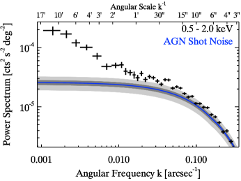
Figure 7: The measured power spectrum $P(k)$ of the brightness fluctuations of the unresolved CXB in XBOOTES in the $0.5-2.0\,\mathrm{keV}$ band. Blue curve shows the AGN shot noise (Sect. 4.3) corrected for the PSF-smearing (App. B). Grey areas illustrate its dependence on the photon index assumed for the flux conversion: the dark gray region shows the effect of the photon index varying from $1.6-1.8$, light grey from $1.4-2.0$. The larger photon-index values result in the larger amplitude of the AGN shot noise.

In Fig. 7 we plot the measured (i.e. the photon shot-noise subtracted) power spectrum in the $0.5-2.0\,\mathrm{keV}$ band. In our current study we are interested primarily on the extragalactic part of the CXB. Our spectral analysis in Sect. 3 suggests that fluctuations below $\sim 1$ keV can potentially be contaminated by the emission of the Galaxy since it contributes about $\sim 40\,\%$ to the unresolved CXB flux in the $0.5-2.0\,\mathrm{keV}$ band (Table 2). However, as we demonstrate in Sect. 5.4.3, the energy spectrum of CXB fluctuations is much harder than that of Galactic emission. This allows us to place an upper limit of about $\approx 7\,\%$ on the contribution of fluctuations of the Galactic emission to the average power in the $0.5-2.0\,\mathrm{keV}$ band at large angular scales ($\sim 3\arcmin-8\arcmin$, Sect. 5.4.3). Furthermore, we compared our results with the those obtained in the $1.0-2.0\,\mathrm{keV}$ band and which is virtually uncontaminated by the emission of the Galaxy and found fully consistent results. We will conduct our analysis in the $0.5-2.0\,\mathrm{keV}$ band for consistency and ease of comparison with previous work.

4.3 Point-source shot noise

Due to their discreteness, point-like X-ray sources (AGN and normal galaxies), give rise to a shot-noise component in the power spectrum (e.g. Cooray & Sheth, 2002). The shot noise is caused by fluctuations of the number of sources per beam and is generally uncorrelated with the LSS signal itself, i.e. it is added linearly to the power spectrum. It is an analog of the photon shot noise (App. C) and for the definition of the power spectrum used in this paper, is independent of the angular frequency.

The shot noise of unresolved point sources can be computed as:

$$P_{\mathrm{SN}}=\int\limits_{S_{\mathrm{Min}}}\mathrm{d}S\;S^{2}\;\frac{\mathrm{d}N}{\mathrm{d}S}\;\left(1-f(S)\right)\text{ .}$$ (18)

where $\mathrm{d}N/\mathrm{d}S$ is the differential $\log N-\log S$ distribution and $f(S)$ is the normalized selection function for point sources (Fig. 12 of K05). Using the $\log N-\log S$ distributions from L12, we obtain for the shot noise of AGN a value of $P_{\mathrm{SN}}^{\mathrm{(AGN)}}\approx 1.25\times 10^{-27}\,\mathrm{(erg\,cm^{-2}s^{-1})^{2}\,deg^{-2}}$ in the $0.5-2.0\,\mathrm{keV}$ band. For this calculation we set the lower flux limit in Eq. (18) to $S_{\mathrm{Min}}=10^{-17}\,\mathrm{erg\,cm^{-2}\,s^{-1}}$, however the result is nearly insensitive to the value of $S_{\mathrm{Min}}$. Although normal galaxies make a comparable contribution to the unresolved CXB flux (Sect. 3.2), due to their steeper $\log N-\log S$ in combination with the $S^{2}$ term in Eq. (18) their shot noise is about $\sim 20$ times lower than the AGN shot noise and in the following it will be neglected.

In instrumental units the AGN shot noise is $\approx 2.49\times 10^{-5}\,\mathrm{(cts\,s^{-1})^{2}\,deg^{-2}}$, using an absorbed power law with a photon-index of $\Gamma=1.7$ (Sect. 3.1.3) for the conversion from physical to instrumental units. The shot noise level is moderately sensitive to the choice of the photon-index. Varying the latter between $\Gamma=1.4$ and $2.0$ (between $1.6$ and $1.8$) results in a variation of the shot noise level by $\sim\pm 25\,\%$ ($\sim\pm 9\,\%$).

The predicted shot noise of unresolved AGN, corrected for the PSF-smearing (App. B), is shown in Fig. 7, along with the uncertainty due to variations of the photon index $\Gamma$ used for the units conversion. From Fig. 7 we can see that at small angular scales, below $\sim 15\arcsec$, the measured power spectrum agrees with the theoretical prediction for AGN shot noise quite well, within $\sim 30\,\%$. However, at larger angular scales, there is a clear LSS signal detected above the shot noise of unresolved AGN. Its origin will be investigated in the next section.

5 The origin of the LSS signal

5.1 The (point-source shot-noise subtracted) power spectrum

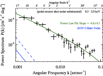
Figure 8: The power spectrum of the detected LSS signal obtained by subtracting the point-source shot-noise from the measured power spectrum shown in Fig. 7. The green solid line shows the power law with the slope of $-0.8$, best-fit to the power spectrum in the $30\arcsec-10\arcmin$ range of angular scales. The blue curves show the two-halo term of unresolved AGN assuming $M_{\mathrm{eff}}=2\times 10^{13}\,\mathrm{M_{\sun}\,h^{-1}}$ (solid line) and $M_{\mathrm{eff}}=1\times 10^{14}\,\mathrm{M_{\sun}\,h^{-1}}$ (dashed line). Note that their average slope is $\approx-2.3$. See Sect. 5.5.1 for details.

In order to characterize the LSS signal we subtract the point-source shot noise from the measured power spectrum in order to obtain the point-source shot-noise subtracted power spectrum. Before the subtraction we renormalize the theoretically computed AGN shot noise from Sect. 4.3 to match the observed power in the $[0.1,0.3[\,\mathrm{arcsec^{-1}}$ frequency range ($\sim 3\arcsec-10\arcsec$). In this range, we can expect that the power spectrum is dominated by the point-source shot noise. The renormalization of the point-source shot noise is needed because the theoretical calculation in Sect. 4.3 is subject to a number of uncertainties, the main of which are: (i) the conversion from physical to instrumental units; (ii) the accuracy of the AGN $\log N-\log S$; (iii) conversion of the survey selection function ($f(S)$) from $0.5-7.0\,\mathrm{keV}$ band to the $0.5-2.0\,\mathrm{keV}$ band; (iv) neglected contribution from normal galaxies. The shape of the theoretical AGN shot noise is determined by the PSF-smearing model, which has an accuracy of $\sim 5\,\%$ for $\gtrsim 2\arcsec$ (App. B). The so computed correction factor is $1.17$ i.e. it is sufficiently close to unity.

The resulting power spectrum of the LSS signal is shown in Fig. 8. A power law fit in the $30\arcsec-10\arcmin$ range of angular scales gives the value of the best fit slope of $-0.8\pm 0.1$. Note that the power spectrum slope depends on the flux cut. This will be further discussed in Sect. 5.4.2.

5.2 Root-mean-square variation

In order to compute the root-mean-square (RMS) variation, we first compute for each observation the variance of the flux map $\mathbf{F}$ in the spatial frequency range of interest:

$$\langle(\delta\mathbf{F})^{2}\rangle_{(k_{1},k_{2})} =\int\limits_{k_{1}}^{k_{2}}\mathrm{d}^{2}k\,P(k)=(\Delta k)^{2}\sum_{k_{1}}^{k_{2}}n(k)\,P(k)\text{ .}$$ (19)

As before, $P(k)$ is the measured power spectrum (Eq. 15). Note that we used Eq. (14) in order to simplify the summation and that the leading coefficient in the above formula depends on the definition of the Fourier transform (Eq. 12).

With $\langle(\delta\mathbf{F})^{2}\rangle$ we can compute the fractional variance $\langle(\delta\mathbf{F})^{2}\rangle/\langle F\rangle^{2}$ where $\langle F\rangle=\Sigma_{i,j}F_{i,j}/\Sigma_{i,j}M_{i,j}$, and its average over all considered observations. The square root of this value gives the average fractional RMS variation in the spatial frequency range $[k_{1},k_{2}]$. In order to estimate the uncertainties, we compute the standard deviation of the fractional variance for individual observations and then use error propagation.

For the entire range of the spatial frequencies $[k_{\mathrm{Min}},k_{\mathrm{Ny}}]$, we obtain the fractional RMS variation of $8\pm 1$ for the $0.5-2.0\,\mathrm{keV}$ band. The AGN shot noise model corrected for the PSF-smearing predicts $\approx 7$, which is fully consistent with the measured value. However, the RMS variation in the full frequency range is dominated by the power at small angular scales (around $\sim 10\arcsec$), where the product of $P(k)$ and the number of modes $n(k)$ is the largest, i.e. it is determined by the AGN shot noise and does not characterize the power at large angular scales.

In order to characterize the latter, we compute the RMS variation for the frequency interval $[0.002,0.006[\,\mathrm{arcsec^{-1}}$ corresponding to the angular scales from $\sim 3\arcmin-8\arcmin$, where the detected LSS signal dominates the power spectrum. Note that the same frequency interval will be used for our spectral analysis in Sect. 5.4.3. We obtain a RMS variation of $(42\pm 2)\,\%$ while our AGN model predicts $\approx 22\,\%$. Subtracting quadratically the latter from the former we obtain the RMS variation of $(36\pm 2)\,\%$ for the LSS signal on the angular scales of arcminutes.

5.3 Potential sources of contamination

The angular scales where the detected LSS signal is particularly pronounced ($\sim 1\arcmin-15\arcmin$) are comparable to the size of the Chandra FOV. There are three main potential sources of contamination at these angular scales: (i) the instrumental background, (ii) large scale spatial non-uniformity of the detector efficiency, and (iii) residual counts in the wings of the PSF from the removed resolved sources.

To investigate significance of the first two factors, we use the instrumental background. In particular, we use both the stowed background data and the XBOOTES data in the $9.5-12.0\,\mathrm{keV}$ band which is entirely dominated by the instrumental background signal. In App. D.2 we compute their power spectra and compare them with each other and with the power spectrum of the unresolved CXB in XBOOTES. We do the comparison both in the units of flux [(cts s^-1)² deg^-2] and of the squared fractional RMS [deg²] (Fig. 19). The former characterizes the significance of the additive contamination (the instrumental background), while the latter characterizes the role of the multiplicative factor (the non-uniformity of the detector efficiency). In both cases, the power spectrum of the instrumental background is by more than an order of magnitude smaller then the power spectrum of the unresolved CXB at any spatial frequency considered here. This excludes a possibility of any significant contamination of the power spectrum of unresolved CXB due to spatial non-uniformity of the instrumental background or detector efficiency.

Residual counts from the resolved sources on average amount to $\approx 2.6$ counts per image in the $0.5-2.0\,\mathrm{keV}$ band (Sect. 2.2.1). This should be compared to the total of $\sim 600$ counts per image of unresolved emission ($\sim 200$ from unresolved CXB and $\sim 400$ from the instrumental background). This is obviously too small to produce fractional RMS of $\approx 40\,\%$ on the $\sim$arcminutes angular scales (Sect. 5.2). We also repeated the entire analysis with the point source exclusion radius of $r=20\arcsec$ and did not find any significant changes in the power spectrum.

Furthermore, the energy spectrum of the LSS signal is much steeper than the energy spectra of the instrumental background and of the resolved sources (Sect. 5.4.3). In the case of the resolved sources the energy spectrum of the residual counts in the wing of the PSF is yet harder than the intrinsic spectrum of sources, due to the energy dependence of the PSF width. This adds further confidence in excluding the contamination by the instrumental effects.

Several other less significant systematic effects, such as the mask effect, are investigated in App. D.

5.4 Observational evidences

If the detected LSS signal is caused by one of the known X-ray source populations, it should be present in the resolved part of the CXB as well. Hence, one should expect that the LSS signal is enhanced if (some fraction of) resolved sources are not removed from the analyzed images.

In the course of our data preparation procedure we remove two types of resolved sources: point and extended sources. The point sources are associated predominantly with AGN and a some small contribution from normal galaxies. As the latter can not be always separated from the former, we investigate their effect together, noting that any LSS signal will be by far dominated by AGN. The extended resolved sources are clusters and groups of galaxies. Below we will investigate possible contribution of each source type to the large scale LSS signal.

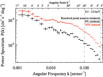
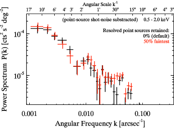
Figure 9: Top: The measured power spectra of the brightness fluctuations in the $0.5-2.0\,\mathrm{keV}$ band for different flux cuts for point source removal. Black crosses: default case used throughout the paper, with all resolved sources removed. Red crosses: the flux cut of $6.2\times 10^{-15}\,\mathrm{erg\,cm^{-2}\,s^{-1}}$ for point sources was applied to the images, retaining $\approx 50\,\%$ of faintest resolved point sources. Bottom: Same as top panel but after subtracting the point-source shot noise (as described in Sect. 5.1). The frequency range used to normalize the point-source shot-noise model is indicated with the two vertical dashed lines in the top panel. The vertical bars are shifted slightly along the x-axis for visualization purposes.

5.4.1 AGN and normal galaxies

In order to investigate the possible role of point sources (AGN and normal galaxies) we construct images keeping $50\,\%$ of faintest resolved point sources in the images. This corresponds to the flux cut of $6.2\times 10^{-15}\,\mathrm{erg\,cm^{-2}\,s^{-1}}$ for the $0.5-2.0\,\mathrm{keV}$ band. With this flux cut, we on average retain 14 resolved point sources per observation, thus approximately doubling the average surface brightness. All other data preparation steps are same as for the default case (Sect. 2).

The power spectra for the two cases are shown in the top panel of Fig. 9. We can see that for the higher flux cut (red crosses) the point-source shot noise noticeably increased, as it should be expected (Eq. 18). In order to study the amplitude of the LSS signal, we subtract the point-source shot noise from the both spectra, as described in Sect. 5.1. The result is shown in the bottom panel of Fig. 9, where we can see that the two spectra are nearly identical. The small difference at small angular scales $\la 2\arcmin$ is likely related to the imperfect shot noise subtraction.

We thus conclude that the LSS signal at large angular scales can not be produced by AGN.

5.4.2 Galaxy clusters & groups

We perform similar analysis for resolved extended sources. Due to their relatively small number in the survey (43 sources, see K05), we compute the power spectrum retaining all resolved extended sources. However, the source area of almost every resolved extended source overlaps with an exclusion area of at least one resolved point source, leading to the loss of about $\sim 50\,\%$ of counts from extended sources. To preserve the extended sources counts, in this analysis we reduced the circular exclusion area to the constant radius of $20\arcsec$ for all resolved point-source sources located within the exclusion area of resolved extended sources. This does not contaminate the signal as resolved point sources do not contribute to the power spectrum in the frequency range of interest, apart from their shot-noise component (also see Sect. 5.4.1).

Since not all of 118 considered XBOOTES fields contain a resolved extended source, we have a possibility to compute the power spectrum for three different field selections. This gives us a more detailed view of the dependence of the power spectrum on the presence or absence of resolved extended sources. Selection A includes all 118 fields. Selection B includes only fields with resolved extended sources. To do the filtering we used the catalog of extended sources from Vajgel et al. (2014, Table 1) which is a result of a more strict selection than the catalog of K05 (Table 1). This selection includes 26 fields containing 29 individual resolved extended sources. Finally, selection C is composed of fields without resolved extended sources. The filtering is based on the extended source catalogs of both Vajgel et al. (2014, Table 1) and K05 (Table 1). Furthermore, we also excluded from this selection fields containing the exclusion area of an extended sources located in an adjacent field. This selection is composed of 76 fields. It can be considered as our control sample, and we expect its power spectrum to be consistent with the default one (from which all resolved sources are removed).

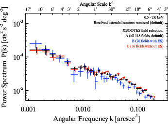
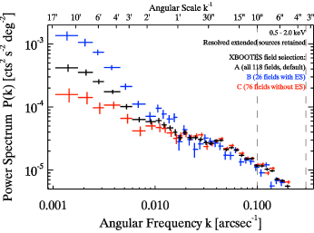
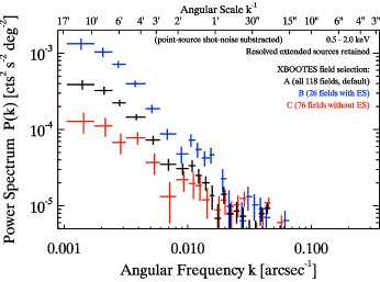
Figure 10: The measured power spectra in the $0.5-2.0\,\mathrm{keV}$ band for different masks and different XBOOTES field selections. Top panel: default mask used throughout the paper, where all resolved sources (point-like and extended) are excluded. Middle panel: special mask described in Sect. 5.4.2, retaining all resolved extended sources. Bottom: Same as middle panel but after subtracting the point-source shot noise (as described in Sect. 5.1). The frequency range used to normalize the point-source shot-noise model is indicated with the two vertical dashed lines in the middle panel. The vertical bars for selection B and C are shifted slightly along the x-axis for visualization purposes.

In Fig. 10 we show the power spectrum for the default mask (top panel, excluding all resolved sources) and the special mask retaining all resolved extended sources (middle and bottom panels) for our three different field selections. From the top panel we can see a good agreement between different field selections On the other hand, in the middle and bottom panels we can see that the power spectrum increases very significantly for angular scales of $\gtrsim 2\arcmin$ for field selection A and B, when we retain all resolved extended source in the images. This strongly suggests that the LSS signal at large angular scales is produced by extended sources (clusters and groups of galaxies), resolved as well as unresolved.

It is interesting to note that not only the amplitude but also the shape of the LSS power spectrum depends on the flux cut for extended sources. While the power spectrum of unresolved CXB has a slope of $-0.8\pm 0.1$ (see also Fig. 8), after we retain resolved extended sources, the best fit slope of the power spectrum changes to $-1.2\pm 0.1$ (see also Fig. 12).

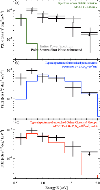
Figure 11: Average power of CXB fluctuations versus energy along with predictions of different spectral models representing the Galactic emission (green, panel (a)), AGN and normal galaxies (blue, panel (b)), and unresolved clusters and groups of galaxies (red, panel (c)). The power is computed from the frequency interval $[0.002,0.006[\,\mathrm{arcsec^{-1}}$ ($\sim 3\arcmin-10\arcmin$) of the measured power spectrum (Eq. 20). The point-source shot noise is subtracted (as in Sect. 5.1), except for the spectrum shown in the upper panel in grey. The points, which are consistent with zero within one standard deviation, are replaced with $1\sigma$ upper limits.

5.4.3 Energy dependence of the CXB fluctuations

The conclusion regarding the association of the LSS signal with clusters and groups of galaxies is further supported by the analysis of the energy spectrum of the CXB fluctuations. To construct the latter, we first compute a series of power spectra in contiguous energy bins in the $0.5-2.0\,\mathrm{keV}$ band and then for each energy bin compute the average power in the range of angular frequencies of interest, subtracting the point-source shot-noise as follows:

$$\langle P(E)\rangle= \frac{\Sigma_{k_{1}}^{k_{2}}\;P(k)}{\Sigma_{k_{1}}^{k_{2}}}-\frac{\Sigma_{k_{3}}^{k_{4}}\;P(k)}{\Sigma_{k_{3}}^{k_{4}}P_{\mathrm{PSF}}(k)}\;\frac{\Sigma_{k_{1}}^{k_{2}}P_{\mathrm{PSF}}(k)}{\Sigma_{k_{1}}^{k_{2}}}\text{ .}$$ (20)

where $[k_{1},k_{2}]$ is the frequency interval for which we used $[0.002,0.006[\,\mathrm{arcsec^{-1}}$ ($\sim 3\arcmin-8\arcmin$), $P_{\mathrm{PSF}}(k)$ is the PSF-smearing model (App. B), and for estimating the point-source shot-noise we use the frequency interval $[k_{3},k_{4}]=[0.1,0.3[\,\mathrm{arcsec^{-1}}$ ($\sim 3\arcsec-10\arcsec$). This definition is equivalent to the re-normalized AGN shot noise model of Sect. 5.1.

The so computed average power is plotted versus energy in Fig. 11. The panel (a) also shows the energy spectrum before subtracting the point-source shot-noise (gray crosses), demonstrating that for the chosen range of angular frequencies its effect is not very significant. Note that taking a square root in Eq. (20) one could obtain a quantity similar to a normal energy spectrum. However, the rather complicated procedure involved in computing the energy spectrum makes the error distribution rather complex and non-Gaussian, so that the conventional spectral fitting techniques may not be directly applied. We therefore chose to consider the energy dependence of the average power expressed in the units of square of the instrumental flux and compare it with predictions of various spectral models. The latter were computed by convolving a spectral model with the energy response of Chandra and squaring the result. The normalizations of the models shown below are arbitrary. In computing the energy spectra of extragalactic sources we assumed the Galactic absorption of $N_{\mathrm{H}}=10^{20}\,\mathrm{cm^{-2}}$ (Kalberla et al., 2005, K05).

To illustrate the amplitude of the possible contamination by the Galactic emission we plot with green lines in panel (a) the APEC model with $T=0.164\,\mathrm{keV}$ (Sect. 3.1.1), normalizing it to the ”flux” of the lowest energy bin ($0.5-0.7\,\mathrm{keV}$). This exercise shows that even in the extremely unlikely case that the lowest energy bin is entirely contaminated by the fluctuations of the surface brightness of the Galactic emission, their contribution to the adjacent $0.7-0.9\,\mathrm{keV}$ energy bin will not exceed $\approx 7\,\%$ and their contribution to the entire $0.5-2.0\,\mathrm{keV}$ band will not be larger than $\approx 7\,\%$. This justifies using the $0.5-2.0\,\mathrm{keV}$ band for fluctuation studies of the extragalactic CXB.

In panel (b) we show a typical energy spectrum of AGN, representing it with a power law with a photon-index of $\Gamma=1.7$ and modified by the Galactic absorption (e.g. Reynolds et al., 2014; Ueda et al., 2014; Yang et al., 2015). Note that the shape of the power law spectrum is not affected by the redshift. We can see that the energy dependence of power predicted by this power law model is significantly harder that the observed dependence. In order to describe the entire energy spectrum with a power law, one would need to assume a very steep slope of $\Gamma\approx 3$, which is not feasible for AGN.

In panel (c) we plot a typical spectrum of clusters and groups of galaxies, for which we used an APEC model modified by the Galactic absorption. For the temperature and redshift we assumed $T=1.4\,\mathrm{keV}$ and $z=0.6$, which are the median values for the unresolved population of clusters and groups of galaxies in XBOOTES (Sect. 3.3). We can see that the model describes reasonable well the observed energy dependence of the average power of the CXB fluctuations.

To conclude, results of this analysis support the conclusion made earlier in this section that the LSS signal is associated with the emission from clusters and groups of galaxies, but not from AGN.

5.5 Comparison with theoretical predictions

5.5.1 AGN

The inability to explain the detected LSS signal by the clustering signal of AGN is not surprising, given our knowledge about their clustering properties. To demonstrate this, we compute the two-halo term for unresolved AGN using Limber’s approximation (assuming small angles, $k^{-1}\ll 1\,\mathrm{rad}$) as follows:

$$P^{(2H)}_{\mathrm{AGN}}(k)= \int\mathrm{d}z\;\left(\frac{\mathrm{d}S}{\mathrm{d}z}\right)^{2}\;\left(\frac{\mathrm{d}^{2}V(z)}{\mathrm{d}z\mathrm{d}\Omega}\right)^{-1}$$

$$\times\;P_{\mathrm{3D,AGN}}\left(k_{\mathrm{3D}}=\tfrac{k}{\beta}\,\tfrac{\alpha}{d(z)},z\right)\text{ .}$$ (21)

where $\mathrm{d}S(z)/\mathrm{d}z$ [erg cm^-2 s^-1 deg^-2] is the AGN flux production rate as function of redshift, defined by Eq. (10) in Sect. 3.3, $\mathrm{d}^{2}V(z)/\mathrm{d}z/\mathrm{d}\Omega$ [Mpc³ h^-3 deg^-2] is the co-moving volume element, and $d(z)$ [Mpc h^-1] is the co-moving distance to redshift $z$ (e.g. Hogg, 1999). The $\alpha$ and $\beta$ are equal to 1, if there is a $2\pi$ in the exponent of the Fourier transform, and they are equal to $2\pi$ otherwise. The AGN 3D power spectrum is computed as following (e.g. Cooray & Sheth, 2002):

$$P_{\mathrm{3D,AGN}}(k_{\mathrm{3D}},z)=b(M_{\mathrm{eff}},z)^{2}\,g(z)^{2}\,P_{\mathrm{lin}}(k_{\mathrm{3D}})\text{ .}$$ (22)

Hereby, $P_{\mathrm{lin}}(k_{\mathrm{3D}})$ [Mpc³ h^-3] is the 3D linear $\Lambda$CDM power spectrum at $z=0$, which we computed using the fitting formulae of Eisenstein & Hu (1998), $g(z)$ is the linear growth function (e.g. Dodelson, 2003), and $b(M_{\mathrm{eff}},z)$ is the AGN linear clustering bias factor, computed with the analytical model of Sheth, Mo & Tormen (2001). For the effective mass $M_{\mathrm{eff}}$ of the DMH, where the AGN reside, we use $2\times 10^{13}\,\mathrm{M_{\sun}\,h^{-1}}$, which is consistent with recent observations up to $z\sim 3$ (e.g. Allevato et al., 2011; Krumpe et al., 2012; Mountrichas et al., 2013).

The predicted two-halo term of unresolved AGN is compared with the measured power spectrum in Fig. 8, which demonstrates that the predicted signal is by nearly two orders of magnitude smaller that the observed one. In order to match the amplitude of the observed LSS signal, one would need to assume the effective DMH mass to be much larger than $M_{\mathrm{eff}}\sim 10^{14}\,\mathrm{M_{\sun}\,h^{-1}}$ for the unresolved AGN population of XBOOTES, which is physically unrealistic (e.g. Cappelluti, Allevato & Finoguenov, 2012; Krumpe, Miyaji & Coil, 2014). Furthermore, the expected power spectrum of the AGN two-halo term is significantly steeper than the observed power spectrum. In the $30\arcsec-10\arcmin$ angular scales range, the former has an average slope of $-2.3$ while the measured power spectrum has a best-fit slope of $-0.8\pm 0.1$ (Fig. 8).

At sub-arcminute angular scales, the shape of the power spectrum is sufficiently well described by the shot noise of unresolved point sources, modified by the PSF smearing effects (Fig. 7). The residuals seen at $\sim 15\arcsec-30\arcsec$ angular scales (Fig. 12) are likely due to the correlation between adjacent Fourier modes caused by the mask. Thus, we do not see any significant evidence for the signal in the power spectrum due to the one-halo term of AGN. This is consistent with the theoretical prediction that low luminosity AGN reside alone in their DMHs (e.g. Leauthaud et al., 2015; Fanidakis et al., 2013). We will defer any quantitative constrains of the halo occupation distribution of AGN based on these data to future work.

5.5.2 Clusters and groups of galaxies

The flux production rate for unresolved clusters and groups of galaxies at the depth of XBOOTES survey peaks at the redshift $z\approx 0.2$ with the median value of $z\approx 0.6$ (Sect. 3.3). At these redshifts, the angular scales of $\lesssim 10\arcmin$ correspond to spatial scales of $\lesssim\$few Mpc, suggesting that the LSS signal is produced by the internal structure of ICM within the same dark matter halo (i.e. their  one-halo term), rather than by the cross-correlation between different objects (two-halo term). This conclusion is supported by the results of analytical calculations of the X-ray power spectrum of groups and clusters of galaxies which demonstrated that at angular scales below $\sim 10\arcmin$ their two-halo term can be neglected (e.g. Komatsu & Kitayama, 1999; Cheng, Wu & Cooray, 2004).

The one-halo term on the angular scales of $\gtrsim 1\arcmin$ is dominated by the nearby objects, located at redshift $z\lesssim 0.1$ (Cheng, Wu & Cooray, 2004). At these redshifts, angular scales of $\sim 5\arcmin-10\arcmin$ correspond to spatial scales of $\sim 0.5-1$ Mpc, i.e. of the order of the $R_{200}$ of a DMH with a mass of $M_{200}\sim 10^{13}-10^{14}\,\mathrm{M_{\sun}}$. Thus, the power spectrum of CXB fluctuations carries information about ICM in cluster outskirts. The shape of the power spectrum is determined by the intrinsic structure of the ICM convolved with the redshift distribution of unresolved clusters and groups of galaxies. The latter depends on the flux cut for the resolved objects, opening prospects for redshift-resolved studies, provided the data of sufficient depth. The normalisation of the power spectrum is proportional to the square of the volume density of clusters and groups of galaxies, making the powers spectrum a sensitive diagnostics of the volume density of these objects.

At small angular frequencies corresponding to large angular scales, the power spectrum is expected to flatten based on the model of Diego et al. (2003), while the model of Cheng, Wu & Cooray (2004) does not show such a strong feature. These angular scales are outside the frequency range studied here, but should become accessible when the full range of scales provided by the XBOOTES ($\sim 3$ deg) and other wide angle surveys will be utilized.

Thus, the power spectrum of CXB fluctuations could potentially provide a new tool to probe the structure of ICM, out to the linear scales beyond $R_{500}$, which are expensive to study with direct imaging observations. This is a valuable possibility. Indeed, due to the complex nature of ICM, theoretical predictions suffer from large uncertainties (e.g. Rosati, Borgani & Norman, 2002; Kravtsov & Borgani, 2012). Depending on the assumed characteristics of gas cooling and heating, the predictions of the structure of ICM and for the clustering strength in particular for the one-halo term can vary dramatically, as analytical studies (e.g. Cheng, Wu & Cooray, 2004) and cosmological hydrodynamical simulations (e.g. Roncarelli et al., 2012) show. For the same reason it is also difficult to accurately predict the total contribution of clusters and groups of galaxies to the CXB (e.g. Roncarelli et al. 2006). The latter is also difficult to achieve observationally, given the insufficient depth of the current measurements of the $\log N-\log S$ of clusters and groups of galaxies, reaching the flux limit of $\sim 10^{-16}\,\mathrm{erg\,cm^{-2}\,s^{-1}}$ at the best (Finoguenov et al., 2015). Due to the steep slope of the $\log N-\log S$ a significant fraction of the total emission from clusters and groups of galaxies is produced by below this flux limit.

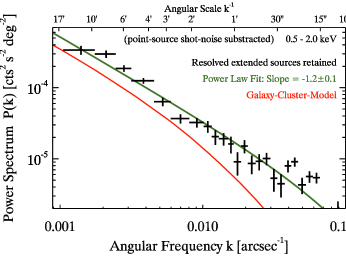
Figure 12: The power spectrum of the brightness fluctuations of the unresolved CXB of XBOOTES in the $0.5-2.0\,\mathrm{keV}$ band, when all resolved extended source are included in the flux map (using our special mask, Sect. 5.4.2). The point-source shot noise is subtracted from the measured power spectrum (Sect. 5.1). The green solid line shows a power law with the slope of $-1.2$, which gives best fit to the observed power spectrum in the angular scale range of $30\arcsec-10\arcmin$. The red curve shows the model for clusters and groups of galaxies based on results of Cheng, Wu & Cooray (2004),

Keeping these uncertainties in mind, we compare our measured power spectrum with theoretical predictions by Cheng, Wu & Cooray (2004), whose calculations are based on a simple model assuming that ICM is in hydrostatic equilibrium. This model is in a good agreement with hydrodynamical simulations of Roncarelli et al. (2006), including more complex physical processes, such as star-formation and supernova feedback. Since Cheng, Wu & Cooray (2004) computed power spectrum of all clusters and groups of galaxies without any flux cut, we will be comparing their results with the corresponding power spectrum from Sect. 5.4.2, including all extended sources. This power spectrum is shown with black symbols in the bottom panel of Fig. 10.

For comparison with our measurement, the power spectrum from Cheng, Wu & Cooray (2004) needs to be converted to flux units, the conversion being achieved by multiplying their power spectrum with the square of the surface brightness of clusters and groups of galaxies. To estimate the latter, we compute the combined surface brightness of resolved extended objects from the catalog of K05 above the flux cut of $S=3\times 10^{-14}\,\mathrm{erg\,cm^{-2}\,s^{-1}}$ ($0.5-2.0\,\mathrm{keV}$ band), obtaining $\sim 1.0\times 10^{-13}\,\mathrm{erg\,cm^{-2}\,s^{-1}\,deg^{-2}}$. We estimate the surface brightness of unresolved clusters and groups of galaxies using the results of Sect. 3.2 and obtain $\sim 2.5\times 10^{-13}\,\mathrm{erg\,cm^{-2}\,s^{-1}\,deg^{-2}}$. Hence, the total surface brightness of clusters and groups of galaxies is $\sim 3.5\times 10^{-13}\,\mathrm{erg\,cm^{-2}\,s^{-1}\,deg^{-2}}$. We convert this to instrumental units with a APEC model modified by the Galactic absorption. For the temperature and redshift we assume $T=2.9\,\mathrm{keV}$ and $z=0.4$, which are the median values for the total population of clusters and groups of galaxies (Sect. 3.3). The conversion depends weakly ($\lesssim 10\,\%$) on the assumed temperature for $T\gtrsim 1.5\,\mathrm{keV}$.

Comparison with our measurement in Fig. 12 shows that the model of Cheng, Wu & Cooray (2004) predicts the shape of the power spectrum remarkably well. However the model normalisation is by a factor of $\approx 2$ smaller. The discrepancy in normalisation is not too dramatic given the number of uncertainties and simplifications involved in the model of Cheng, Wu & Cooray (2004). The easiest explanation for it could be the method for computing the model normalisation we used above. Indeed, the estimate of the surface brightness of unresolved clusters and groups of galaxies depends on the assumed slope of their $\log N-\log S$ distribution, for which we used Ebeling et al. (1997) results. As explained in Sect. 3.2, if we increased the slope of the XLF of Ebeling et al. (1997) by $\sim 10\,\%$, the flux from unresolved clusters and groups of galaxies would increase by $\sim 50\,\%$ and the Cheng, Wu & Cooray (2004) model would match our measured LSS signal within $\sim 30\,\%$ accuracy.

The power spectrum of clusters and groups of galaxies can be modified significantly by non-gravitational effects (e.g.  Fig. 3 in Cheng, Wu & Cooray, 2004). Cooling and heating of the ICM can significantly affect its surface brightness distribution which can change the power spectrum by as much as an order of magnitude. Therefore the agreement between a simple semi-analytical model and our data is remarkable and demonstrates the potential of the power spectrum of CXB fluctuations in constraining theoretical models.

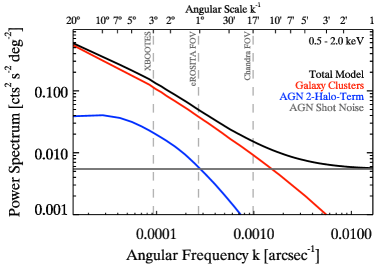
Figure 13: Predicted power spectrum of the brightness fluctuations of the CXB in the SRG/eROSITA all-sky survey in the $0.5-2.0\,\mathrm{keV}$ band for the sky-averaged case. The curves are: clustering signal of (resolved and unresolved) galaxy clusters (red curve), two-halo term (blue curve), and shot-noise level (gray line) for AGN, and the sum of all components (black curve). The PSF-smearing is not taken into account but should only become important at angular scales below $\sim 2\arcmin$. The vertical dashed lines indicate the size of the instruments’ FOVs and of the XBOOTES survey. The power spectrum is shown in instrumental units and we used the response matrix of SRG/eROSITA (erosita_iv_7telfov_ff.rsp) for the conversion.

6 SRG/eROSITA forecast

The upcoming all-sky survey of SRG/eROSITA (eRASS, $\sim$2017-2021) will lead us in a new area of high precision LSS studies with $\sim 3$ million of resolved AGN (Kolodzig et al., 2013b, a; Hütsi et al., 2014) and $\sim 100\,000$ galaxy clusters (Merloni et al., 2012). However, eRASS will also produce an all-sky map of the unresolved CXB with the usable area of the order of $\sim 34\,000$ deg² (excluding the Galactic plane, $|b|>10^{\circ}$) and the point-source sensitivity of $S_{0.5-2.0\,\mathrm{keV}}\approx 1.1\times 10^{-14}$ $\mathrm{erg\,cm^{-2}\,s^{-1}}$ (sky average). With the FOV-averaged PSF of $\sim 30\arcsec$ (Merloni et al., 2012), it will cover a very large range of angular scales, from $\sim$arcminute to the full sky. Given the PSF size, a point-source exclusion region radius of $140\arcsec$ would be sufficient, leaving unmasked about $\approx 60\,\%$ of the sky area ($\sim 21\,000$ deg²).

Due to the survey strategy of eRASS, it will also have deep survey regions at the northern and southern ecliptic poles (NEP and SEP, Merloni et al., 2012). These regions are of particular interested since they will offer a comparable point-source sensitivity as the largest surveys of the current generation of X-ray telescopes, e.g. XBOOTES ($\sim 9$ deg², Chandra, K05), Stripe 82 ($\sim 31$ deg², XMM-Newton, LaMassa et al., 2016), and XXL ($\sim 25\times 2$ deg², XMM-Newton, Pierre et al., 2011) but with a much larger sky area of $\sim 100$ deg² or even up to $\sim 1000$ deg². Further, the angular resolution within these regions can be improved by a factor of $\sim$two by only using the central part of the eROSITA-FOV, making it comparable to the the angular resolution of XMM-Newton.

Given these features of eRASS, it will permit not only to dramatically broaden the range of the angular scales, but also to improve the accuracy of the measurement of the surface brightness fluctuations of the unresolved CXB, increasing in the S/N ratio by a factor of about $\sim 50$, as compared to XBOOTES data. This will allow one to test clustering models of unresolved AGN and galaxy clusters to an unprecedented precision. Importantly, these studies do not need redshifts of objects i.e. are independent on the optical follow-up studies.

In Fig. 13 we show the expected power spectrum of CXB fluctuations in eRASS in the $0.5-2.0\,\mathrm{keV}$ band for the sky-averaged case. The shot-noise level (gray line) and two-halo term (blue curve) of unresolved AGN were computed as described in Sect. 4.3 and 5.5.1, respectively, using the sky-averaged point-source sensitivity of eRASS. The power spectrum of (resolved and unresolved) clusters of galaxies (red curve) is based on the theoretical prediction by Cheng, Wu & Cooray (2004), which was normalized as described in Sect. 5.5.2. One can see from Fig. 13 that the CXB brightness fluctuations will be dominated by the clustering signal of clusters and groups of galaxies at angular scales larger than $\sim 10\arcmin$. At smaller angular scales the dominant contribution will come from AGN. The unresolved AGN population of eRASS will be located at a median redshift of $z\approx 1.2$ and will have a moderate median luminosity of $L_{0.5-2.0\,\mathrm{keV}}\sim 10^{43.4}\,\mathrm{erg\;s^{-1}}$. Given the angular resolution of SRG/eROSITA and the expected high S/N of the power spectrum, one should be able to measure or constrain the one-halo term of AGN at the angular scales of $\sim 1\arcmin-10\arcmin$ to a high precision. This may permit us to finally measure or constrain the mean occupation number of AGN per DMH, which is an important parameter for the AGN triggering and fueling theories which has not yet been reliably constrained (e.g. Cappelluti, Allevato & Finoguenov, 2012; Krumpe, Miyaji & Coil, 2014; Leauthaud et al., 2015).

7 Summary

Surface brightness fluctuations of the unresolved CXB present a great opportunity to study faint source populations which are yet beyond the reach of more conventional studies of resolved sources. The renaissance of this field was facilitated by the fact that wide angle X-rays surveys covering tens of deg² have been undertaken by the modern X-ray telescopes aboard Chandra and XMM-Newton, featuring superb angular resolution (e.g. Brandt & Alexander, 2015). In the work reported in this paper we used the data of XBOOTES, the presently largest continuous Chandra survey covering the area of $\sim 9$ deg², to conduct the most accurate measurement to date of the brightness fluctuations of unresolved CXB in the angular scales ranging from $\sim 3\arcsec$ to $\sim 17\arcmin$.

The XBOOTES survey with its average exposure of $\sim 5$ ksec per field has an average point-source sensitivity of $\sim 2\times 10^{-15}\,\mathrm{erg\,cm^{-2}\,s^{-1}}$ in the $0.5-2.0\,\mathrm{keV}$ band (K05) and an average extended-source sensitivity of $\sim 3\times 10^{-14}\,\mathrm{erg\,cm^{-2}\,s^{-1}}$ (Sect. 3.2). Given these flux limits, unresolved AGN and normal galaxies make the major contribution to the surface brightness of the unresolved CXB, accounting each for $\sim 30\,\%$, with the galaxy clusters making a more modest contribution at the level of $\sim 6-8\,\%$ (Sect. 3.2). However, estimates for normal galaxies and galaxy clusters are highly uncertain, thus explaining that about $\sim 1/3$ of the CXB flux remains unaccounted for in this calculation. At a point-source sensitivity level of $\sim 10^{-15}\,\mathrm{erg\,cm^{-2}\,s^{-1}}$ normal galaxies are not expected to contribute significantly to the unresolved CXB fluctuations. The unresolved AGN have a median redshift of $z\sim 1.0$ and median luminosity of $L_{0.5-2.0\,\mathrm{keV}}\sim 10^{42.6}\,\mathrm{erg\;s^{-1}}$ (Sect. 3.3). The unresolved galaxy clusters are about twice as close, with a median redshift of $z\sim 0.6$ (flux-weighted mean of $\left<z\right>\sim 0.3$) and have comparable median luminosity of $L_{0.5-2.0\,\mathrm{keV}}\sim 10^{42.7}\,\mathrm{erg\;s^{-1}}$. With the standard scaling relations, these numbers correspond to an ICM temperature of $T\sim 1.4\,\mathrm{keV}$, and a DMH mass of $M_{500}\sim 10^{13.5}$ (Sect. 3.2).

After masking out resolved (point and extended) sources, we obtained the power spectrum of surface brightness fluctuations of unresolved CXB in the $3\arcsec-17\arcmin$ range of angular scales (Fig. 7). At sub-arcminute angular scales, the obtained power spectrum is consistent with the predicted point source shot noise of unresolved AGN, corrected for the PSF-smearing. However, at the angular scales exceeding $\gtrsim 1\arcmin$ we detect a clear and highly statistically significant LSS signal above the AGN shot noise. After subtracting the point-source shot noise, we obtain the power spectrum of the LSS signal, which follows an approximate power-law shape with the slope of $-0.8\pm 0.1$ (Fig. 8) and has normalization corresponding to the fractional RMS variation of $(36\pm 2)\,\%$.

The detected LSS signal is by almost two orders of magnitude stronger than that expected from the AGN two-halo term (Fig. 8). We present strong evidence that it is associated with the ICM of unresolved galaxy clusters, namely with their one-halo term. In particular, we show that the LSS signal is not present in the power spectrum of resolved AGN (Fig. 9), and it is much enhanced when resolved galaxy clusters are retained on the images (Fig. 10). The energy dependence of the mean power of the CXB fluctuations at a $\sim$few arcmin angular scales is consistent with the energy spectrum of an optically thin plasma with temperature of $T=1.4$ keV redshifted to $z=0.6$, corresponding to the average ICM temperature and median redshift of unresolved galaxy clusters in the XBOOTES survey (Fig. 11). The shape of the power spectrum can be remarkably well described by the model of Cheng, Wu & Cooray (2004), although the normalization of the theoretical spectrum is by about a factor of $\approx 2$ smaller than observed (Fig. 12).

The power spectrum of fluctuations of unresolved CXB carries information about the ICM structure in the outskirts (out to $\sim R_{200}$) of nearby ($z\lesssim 0.1$) clusters and groups of galaxies (e.g. Cheng, Wu & Cooray, 2004). These scales are difficult to reach by conventional studies based on the surface brightness distribution of individual and usually relatively nearby objects. The shape of the observed power spectrum is determined by the spatial structure of ICM, and the redshift distribution of clusters and groups of galaxies, while its normalization is proportional to the square of their volume density. This underlines the enormous diagnostic potential of the unresolved CXB fluctuation analysis.

Appendix A Spectral model of the instrumental background

In order to study the energy spectrum of the unresolved CXB, one needs a spectral model for the instrumental background. We create such a model using the ACIS-I stowed background data. The data is processed as recommended by the corresponding CIAO threads. We fit its energy spectrum between $0.5$ and $10.0\,\mathrm{keV}$ with a spectral model consisting of a power law with six Gaussians to account for the instrumental emission lines of Al K_α, Si K_α, Au K_α,β, Ni K_α and Au L_α, (Baganoff, 1999, e.g. Fig. 3, left panel) and for an additional feature around $8.3\,\mathrm{keV}$. The stowed background spectrum and the best-fit model is shown in Fig. 14. The model describes the energy spectrum of the instrumental background with the accuracy sufficient for this study, which main purpose is decomposition of the CXB spectrum below 2 keV into Galactic and extragalactic components and measurement of their fluxes. We therefore use this model to fit the spectrum of the unresolved CXB in XBOOTES in Sect. 3.1.1. In the spectral fit to the XBOOTES data we fixed the slope of the power law of the instrumental background and the parameters of the two low energy lines as indicated in Table 5 at the best-fit values to the stowed background data. Other parameters were left free. Their best-fit values are listed in Table 5.

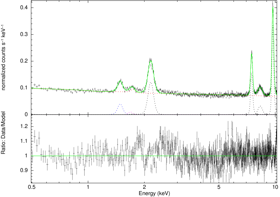
Figure 14: Energy spectrum of the ACIS-I stowed background along with the instrumental background model. Black crosses: data points with one standard deviation as error-bars. Green Curve: Total background model. Dotted Curves: single components of the model (see Table 5).

Table 5: Best-fit values of the instrumental background model (pink curve in Fig. 3) obtained in the spectral fit to the unresolved CXB in XBOOTES (Sect. 3)

Component-Name	Parameter	Value
powerlaw	Photon Index	0.107 (fixed)
1. Gaussian	Center	1.490 keV
(Al Kα)	Width	19.4 eV (fixed)
2. Gaussian	Center	1.678 keV (fixed)
(Si Kα)	Width	0.1 eV (fixed)
3. Gaussian	Center	2.162 keV
(Au Kα,β)	Width	52.0 eV
4. Gaussian	Center	7.473 keV
(Ni Kα)	Width	11.8 eV
5. Gaussian	Center	9.700 keV
(Au Lα)	Width	35.0 eV
6. Gaussian	Center	8.294 keV
	Width	185.1 eV

The width is the standard deviation of the Gaussian. The fixed values are from the fit of the ACIS-I stowed background spectrum (Fig. 14).

Table 6: Surface brightness of the instrumental background of XBOOTES in the $0.5-2.0\,\mathrm{keV}$ band determined from the spectral fit and using the background map.

Estimated based on	Value
	[cts s-1 deg-2]
Spectral fit (Sect. 3.1.1)	$1.548\pm 0.004$
Background maps (Sect. 2.4)	$1.55\pm 0.01$

One can see in Fig. 3 that the instrumental background model has higher continuum level than the CXB, which makes the estimate of the CXB flux sensitive to the slope of the power law component of the background model. Therefore it is reassuring that the surface brightness of the instrumental background obtained from the spectral fit of the XBOOTES data is consistent with the average surface brightness of the background maps $\mathbf{C}^{\mathrm{BKG}}$ obtained with the help of the stowed data in Sect. 2.4, see Table 6. The latter uses the method of H06 to estimate the background spectrum normalisation from the $9.5-12.0\,\mathrm{keV}$ band (Eq. 3), whereas for the former we fit the data below $10.0\,\mathrm{keV}$.

Appendix B PSF-smearing model

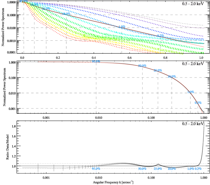
Figure 15: Top: The azimuthally averaged power spectra of Chandra PSF (dotted curves) for different offset angles from $0\arcmin$ (black) to $11\arcmin$ (red) with the step of $1\arcmin$ for the $0.5-2.0\,\mathrm{keV}$ band. The thickness of the curves indicates the weight used in the averaging over offset angles. Top and Middle: Average power spectrum of the PSF of Chandra ACIS-I (gray crosses, average over all offset angles and CCDs) and the PSF-smearing model (red curve, Eq. 23). Bottom: Ratio between the average PSF power spectrum and the PSF-smearing model.

Table 7: Parameters of the PSF-smearing model (Eq. 23) in the $0.5-2.0\,\mathrm{keV}$ band.

Symbol	Value	Unit
$k_{b}$	0.134	arcsec-1
$\alpha_{1}$	-4.740	arcsec
$\beta_{1}$	0.020	-
$\alpha_{2}$	-3.270	arcsec
$\beta_{2}$	-0.180	-

The PSF of Chandra will smooth out any fluctuation signal caused by source photons on the angular scales smaller than its size. Note that fluctuation caused by instrumental background are not affected. This leads to a drop of the source power spectrum $P_{Scr}(k)$ amplitude at small scales (e.g.  Fig. 7). Since the shape of the PSF is rather complex and changes with the offset angle ($\theta$) and azimuthal angle ($\phi$) from the focal point (see Fig. 1), one can not derive a simple analytical expression to describe this effect. Therefore, we use an empirical approach and compute an average PSF power spectrum from the measured PSF power spectra of our PSF simulations in Sect. 2.2 for the $0.5-2.0\,\mathrm{keV}$ band. Thereby, we first average over all CCDs and then compute a weighted average over all offset angles. For the weights we use the surface area of the annulus of each offset angle. We show the average PSF power spectrum in Fig. 15 (grey crosses) along with our simple empirical PSF-smearing model (red curve), which is a broken exponential function in the base of ten:

$$\log_{10}\left[P_{\mathrm{PSF}}(k)\right]=\begin{cases}\alpha_{1}\,k+\beta_{1}&\text{for $k\leq k_{b}$},\\ \alpha_{2}\,k+\beta_{2}&\text{for $k\geq k_{b}$}.\end{cases}$$ (23)

The parameters of the model are listed in Table 7. Our model is able able to describe the PSF power spectrum up to a frequency of $k\approx 0.9\,\mathrm{arcsec^{-1}}$ ($\gtrsim 1.1\arcsec$, $\gtrsim 2$ image pixels) with an accuracy of $\approx 5\%$, which is sufficient for the given S/N of our fluctuation measurements. We can see also in Fig. 17 that our PSF-smearing model is able to describe well the measured power spectrum in the entire range of angular scales of interest.

Appendix C Photon shot noise

When measuring the angular fluctuations of the unresolved CXB via Fourier analysis, we have to take into account that the source power spectrum $P_{\mathrm{Scr}}(k)$ is superimposed by the photon shot noise $P_{\mathrm{Phot.SN}}$ in our measured power spectrum: $\langle|\widehat{\delta F}(k)|^{2}\rangle=P_{\mathrm{Src}}(k)+P_{\mathrm{Phot.SN}}$. In the ideal case the shot noise is flat and independent of the Fourier frequency. Its mean amplitude is inversely proportional to the total number of counts and it contributes to the statistical noise in the source power spectrum: $\sigma_{P_{\mathrm{Scr}}}(k)\propto P_{\mathrm{Src}}(k)+P_{\mathrm{Phot.SN}}$.

C.1 Estimators

Below we discuss three different photon shot-noise estimators.

C.1.1 Analytical estimate

Ignoring the effects of the mask (Sect. D.1) and vignetting, one can use a simple analytical expression to estimate the shot-noise amplitude, which we derive here for completeness. For simplicity we use in the following a single index ($j$) for the summations over all pixels $N$ of a 2D map. Based on our definition in Sect. 4.1, we can write the measured power spectrum as following:

$$\left\langle|\widehat{\delta F}(\mathbf{k})|^{2}\right\rangle= \dfrac{1}{\Omega}\!\left\langle\!\left(\sum_{j}^{N}\delta F_{j}\,\mathrm{e}^{-2\pi\mathrm{i}\,\mathbf{r}_{j}\mathbf{k}}\right)\!\!\left(\sum_{l}^{N}\delta F_{l}\,\mathrm{e}^{+2\pi\mathrm{i}\,\mathbf{r}_{l}\mathbf{k}}\right)\!\right\rangle$$

$$= \dfrac{1}{\Omega}\!\left\langle\sum_{j}^{N}\delta F_{j}^{2}\right\rangle$$

$$+\dfrac{1}{\Omega}\!\left\langle\sum_{j}^{N}\sum_{l\neq j}^{N-1}\delta F_{j}\,\delta F_{l}\,\mathrm{e}^{-2\pi\mathrm{i}\,\mathbf{k}(\mathbf{r}_{j}-\mathbf{r}_{l})}\right\rangle\text{ .}$$

The second term represent the actually source power spectrum $P_{\mathrm{Scr}}(k)$, whereas the first term is the shot noise. We can reduce the first term further to:

$$\left\langle\sum_{j}^{N}\delta F_{j}^{2}\right\rangle =\sum_{j}^{N}\left\langle\delta F_{j}^{2}\right\rangle=\sum_{j}^{N}\left(\left\langle F_{j}^{2}\right\rangle-\langle F_{j}\rangle^{2}\right)$$

$$=\sum_{j}^{N}\sigma^{2}(F_{j})=\sum_{j}^{N}\dfrac{\sigma^{2}(C_{j})}{E_{j}^{2}}\approx\sum_{j}^{N}\dfrac{C_{j}}{E_{j}^{2}}\text{ .}$$

Here, we use the fact that $\delta F_{j}=F_{j}-\langle F_{j}\rangle$ and $F_{j}=C_{j}/E_{j}$ and that the variance $\sigma^{2}(x)$ of a Poissonian-distributed quantity $x$ is equal to its mean. Since we do not know the actually mean of $C_{j}$ we approximate it with its own value. Based on this derivation, we define our shot noise estimate as following:

$$P_{\mathrm{Phot.SN}} =\dfrac{1}{\Omega}\sum_{j}^{N}\dfrac{C(\mathbf{r}_{j})}{E^{2}(\mathbf{r}_{j})}\text{ .}$$ (24)

When we are using the average exposure map (Eq. 2) for computing the fluctuation map $\delta\mathbf{F}$, the definition changes to:

$$P_{\mathrm{Phot.SN}} =\dfrac{1}{\Omega}\dfrac{\sum_{j}^{N}C(\mathbf{r}_{j})}{\langle E\rangle^{2}}\text{ .}$$

We refer to both definitions as the analytical shot-noise estimate, which is our default shot-noise estimate.

Note that this definition is only valid for the total-count map $\mathbf{C}_{X}^{\mathrm{Total}}$ (Sect. 2.4). For the background-subtracted map $\mathbf{C}_{X}^{\mathrm{CXB}}$ (Eq. 4) one has to explicitly add the shot noise due to the instrumental background events, as the flux of the the latter was subtracted from $C(\mathbf{r}_{j})$ in Eq. 24:

$$P_{\mathrm{Phot.SN}}^{\mathrm{(CXB)}} =P_{\mathrm{Phot.SN}}+P_{\mathrm{Phot.SN}}^{\mathrm{(BKG)}}\text{ ,}$$

with (using Eq. 3)

$$P_{\mathrm{Phot.SN}}^{\mathrm{(BKG)}} =\dfrac{\sum_{j}^{N}C_{j}^{\mathrm{Stow}}}{\Omega\,\langle E^{\mathrm{Stow}}\rangle^{2}}\cdot\left(\dfrac{\sum_{j}^{N}\,C_{9.5-12.0\,\mathrm{keV}}^{\mathrm{Total}}}{\sum_{j}^{N}\,C_{9.5-12.0\,\mathrm{keV}}^{\mathrm{Stow}}}\right)^{2}\text{ .}$$

C.1.2 High-frequency based estimate

The high-frequency based shot-noise estimate uses the fact that at very high frequencies the measured power spectrum converges eventually to the shot-noise amplitude (Sect. B). Hence, we can estimate the shot noise by taking the average ($P^{\mathrm{(HF)}}_{\mathrm{Phot.SN}}$) of the power spectrum for some frequency interval $[k^{\mathrm{(HF)}}_{\mathrm{min}},k^{\mathrm{(HF)}}_{\mathrm{max}}]$. It is natural to choose the upper limit at the Nyquist-Frequency: $k^{\mathrm{(HF)}}_{\mathrm{max}}=k_{\mathrm{Ny}}$. The choice of the lower limit is somewhat arbitrary and depends on the amplitude and the slope of the power spectrum of the signal. We use $k^{\mathrm{(HF)}}_{\mathrm{min}}=k_{\mathrm{Ny}}\times 0.80\approx 0.81\,\mathrm{arcsec^{-1}}$. With this choice, the interval encapsulates angular scales of the size $\approx 2.5$ ACIS-I CCD pixels or smaller ($\leq 1.2\arcsec$). At these scales the amplitude of the source power spectrum is suppressed by more than $500$ times due to PSF-smearing (Fig. 15) and the shot-noise-subtracted power spectrum in the $0.5-2.0\,\mathrm{keV}$ band is more than $\sim 2000$ times smaller than the shot-noise amplitude itself (computed using the analytical shot-noise estimate). Therefore, within this frequency interval the source power spectrum can be neglected (cf. Fig. 17). We also tested larger and smaller values for $k^{\mathrm{(HF)}}_{\mathrm{min}}$ and find that $k^{\mathrm{(HF)}}_{\mathrm{min}}=k_{\mathrm{Ny}}\times 0.80$ is a good compromise . Furthermore, using $k^{\mathrm{(HF)}}_{\mathrm{min}}=k_{\mathrm{Ny}}\times 0.40\approx 0.41\,\mathrm{arcsec^{-1}}$ we obtain the the shot-noise-subtracted power spectrum which is nearly identical to the default one in the frequency range of interest, at frequencies $\lesssim 0.3\,\mathrm{arcsec^{-1}}$. It should be noted that this shot-noise estimator requires the maximal angular resolution of Chandra, i.e. needs the image pixel binning of one.

As we show in the Sect. C.2, the high-frequency based estimate works as well as the analytical estimate and produces results compatible with the latter. The caveat is that it may be subject to contamination by the signal, i.e. prone to overestimating the shot-noise level if there is this still a significant source signal at frequencies $\ga k^{\mathrm{(HF)}}_{\mathrm{min}}$. Nevertheless, this estimate serves as a useful independent test for the analytical estimate.

C.1.3 Observation-splitting based estimate

The observation-splitting shot-noise based estimate, also called the $A-B$ technique, was introduce by Kashlinsky et al. (2005) for infrared data and was also used for X-ray data (e.g. Cappelluti et al., 2013; Helgason et al., 2014). Hereby, one splits the observation into even and odd time-frames (or events) and creates a fluctuation map for each subset ($\delta\mathbf{F}_{A}$ for even frames and $\delta\mathbf{F}_{B}$ for odd frames). The difference between these two maps should be free of any source or instrumental signal which is steady in time, because both subsets were observed nearly simultaneously, and only contain the random noise of the observation. Hence, the measured power spectrum $P^{\mathrm{(OS)}}_{\mathrm{Phot.SN}}$ of the difference $\delta\mathbf{F}_{D}=(\delta\mathbf{F}_{A}-\delta\mathbf{F}_{B})/2$ should represent the shot noise for this observation. For the shot-noise-subtracted power spectrum, we take the statistical uncertainties of the measured power spectrum and of $P^{\mathrm{(OS)}}_{\mathrm{Phot.SN}}$ into account and use the normal error propagation.

As we show in the Sect. C.2, observation-splitting based estimate gives in average consistent results in comparison to the analytical estimate. However, a major concern with this estimate is that this estimate is itself subject to noise. Combined with correlations between different Fourier modes caused by the mask effect this leads to appearances of irregularities in the resulting shot-noise-subtracted power spectrum. This can been seen for instance in Fig. 17 (lower panels, green crosses) for in the interval of $0.5\lesssim k[\mathrm{arcsec^{-1}}]\lesssim 0.7$, where the observation-splitting based estimate leads to a significant underestimation of the power spectrum. This also makes the observation-splitting based estimate somewhat less reliable in comparison to the analytical or high-frequency based estimate. However, it serves as another independent probe of the photon shot-noise level.

C.2 Comparison of different estimators

In the following, we compare different shot-noise estimates. Thereby, we focus mostly on the high frequency part of the power spectrum, where the source power spectrum is of the order of the shot-noise amplitude or smaller. For a better visualization, we show the power spectrum in linear scale and use a linear binning, although all calculations were performed with the unbinned power spectrum.

C.2.1 The $9.5-12.0\,\mathrm{keV}$ band

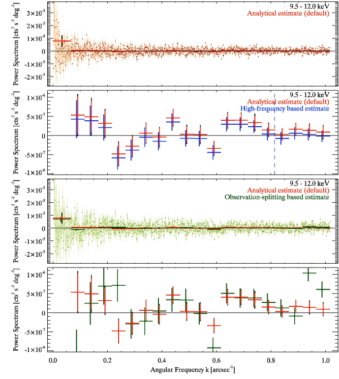
Figure 16: Photon-shot-noise-subtracted power spectrum $P(k)$ (Eq. 15) in the $9.5-12.0\,\mathrm{keV}$ band. Red crosses in all panels were obtained using our default method of analytical shot-noise estimate (Eq. 24). Blue crosses in the two upper panels were computed using the high-frequency based estimate (Sect. C.1.2). Green crosses in the two lower panels were obtained using the observation-splitting based estimate (Sect. C.1.3). The colored error-bars show the standard deviation due to error propagation of all binned frequencies. The black error-bars show the standard deviation of the sample mean of all binned frequencies. Vertical blue dashed line shows the lower limit $k^{\mathrm{(HF)}}_{\mathrm{min}}$ used to compute the high-frequency based estimate.

The power spectrum in the $9.5-12.0\,\mathrm{keV}$ band is ideal for evaluating the photon shot-noise estimators. Since the effective area of Chandra mirrors is virtually zero at these energies, all registered events are due to the instrumental background. At small angular scales the power spectrum of the instrumental background is flat and consists of the photon shot-noise only. This fact can be used to evaluate and compare our shot-noise estimators.

The photon shot-noise subtracted power spectra are plotted in Fig. 16. As one can see, there are quite significant fluctuations in the binned spectra. They are caused by the correlation between nearby Fourier modes caused by the mask effect. This correlations is not accounted for in computing the errors and leads to seemingly statistically significant deviations from the zero in the binned power spectrum. In Fig. 16 we also show in black colour the RMS of power in individual Fourier modes computed within the broad frequency bins. They somewhat higher than the theoretical error bars computed as described above (Eq. 16).

The lowest frequency bin contains a real signal due to the slightly non-uniformity of the instrumental background at large scales, which also can be seen in the power spectrum of the stowed background map (Sect. D.2, Fig. 19). Therefore, we exclude the frequencies $<0.02\,\mathrm{arcsec^{-1}}$ from the following evaluation.

To compare different estimates we compute the sample mean and RMS deviation for the quantity $Z(k)=P(k)/\sigma_{P(k)}$. Since the unbinned power spectrum has more than $1000$ Fourier frequencies, the average of $Z(k)$ follows Gaussian distribution and, in the ideal case, has the mean zero with a RMS deviation of one. We measure a RMS deviation of $\approx 1.14$ for all shot-noise estimates and the sample mean of $0.05\pm 0.03$, $0.00\pm 0.03$ and $0.08\pm 0.03$ for the analytical, high-frequency based, and observation-splitting based estimates, respectively. This calculation shows somewhat inferior quality of the observation-splitting based estimate which is also confirmed by the visual inspection of Figs. 16 and 17. We choose the analytical estimator as our default one for the analysis in this paper.

C.2.2 The $0.5-2.0\,\mathrm{keV}$ band

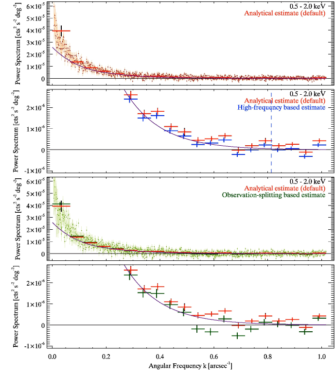
Figure 17: Same as Fig. 16 but for the $0.5-2.0\,\mathrm{keV}$ band. Purple solid curve shows AGN shot-noise model (Sect. 4.3) multiplied by the PSF-smearing model (Sect. B).

In Fig. 17 we show the photon shot-noise subtracted power spectrum $P(k)$ for the $0.5-2.0\,\mathrm{keV}$ band for our three shot-noise estimators. We also plot the AGN shot-noise model (Sect. 4.3), multiplied with the PSF-smearing model (Sect. B). One can see good agreement of the data with the model in the entire frequency range. This plot justifies neglecting the contribution of the signal for the frequencies of $>k_{\mathrm{Ny}}\times 0.80\approx 0.81\,\mathrm{arcsec^{-1}}$, which were used to compute the high-frequency based estimate. It also demonstrates that our AGN shot-noise model combined with the PSF-smearing model is able to describe the measured power spectrum up to the highest frequencies.

Finally, we note that the differences between different photon shot-noise estimators are significant only at highest frequencies. For the analysis presented in this paper, which is focused at frequencies $\lesssim 0.3\,\mathrm{arcsec^{-1}}$ these differences are unimportant.

Appendix D Other systematic effects

Below we discuss several less significant systematic effects having impact on the resulting power spectrum.

D.1 Mask effect

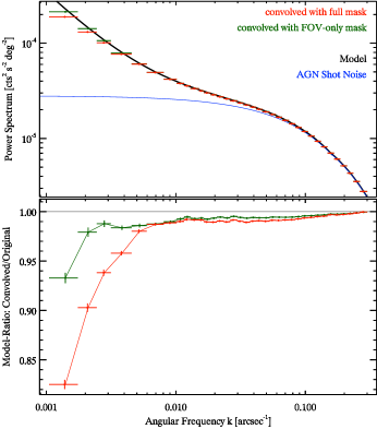
Figure 18: The impact of the mask effect on the power spectrum. Top: The simulated power spectra after two different masks were applied to the simulated images, which are based on our input model (black curve). Also shown is the AGN shot noise model (blue curve). Bottom: The ratio of the simulated power spectra to our input model. The data points of different color show the effect of two different masks: the FOV-only mask (green) and the full mask taking into account the resolved sources and CCD gaps (red).

The measured power spectrum is a convolution of the true power spectrum with a that of the window function, because the analysed image has a finite size and is modified by the mask excluding the regions corresponding to resolved sources, CCD gaps and bad pixels. This alters the power spectrum and leads to correlation of adjacent Fourier modes. We refer to these modifications with the term mask effect. Here, we estimate how this effect distorts the source power spectrum in the considered frequency range of $0.001-0.300\,\,\mathrm{arcsec^{-1}}$ ($\sim 3\arcsec-17\arcmin$).

To compute the mask effect we perform simulations as follows. We construct a model power spectrum consisting of the shot-noise of unresolved AGN and a power law component $P\propto k^{-1.3}$ corresponding to the LSS signal, both multiplied by the PSF-smearing function. From this power spectrum we create a two-dimensional Fourier-image assuming random and uniformly distributed phases and perform an inverse Fourier transform to compute the corresponding image. The resulting image is multiplied by the mask. This is repeated for each Chandra observation, each time using the real mask for that observation. From the produced set of images we compute the average power spectrum following same procedures as were applied to the real data. This procedure was repeated $50$ times and the result was averaged to produce the final power spectrum which was then compared with the input model.

The result of these simulations is shown in Fig. 18. One can see that due the mask effect the power spectrum is suppressed by less than $\sim 20\,\%$ at the lowest considered frequency bin and at the frequencies of $\gtrsim 4\times 10^{-3}\,\,\mathrm{arcsec^{-1}}$ it is suppressed by less than $\sim 2\,\%$. This means that the measured power spectrum is a reasonably good representation of the true power spectrum of the signal. Due to the complexity of the inverse problem, we chose not to correct the power spectrum for the mask effect. Instead, these effects can be straightforwardly taken into account when fitting the measured spectrum with theoretical models.

D.2 Instrumental background

At the flux limit of XBOOTES survey, the instrumental background accounts for $\sim 2/3$ of the unresolved emission, therefore its non-uniformity can significantly contaminate the power spectrum. In addition to the non-uniform distribution of the instrumental background over the detector, its surface brightness distribution may be affected by the large scale non-uniformity of the detector efficiency (if any). Thus, investigation of the stowed background data can be also used to constrain the amplitude of the latter. The power spectrum of the stowed background ($\mathbf{C}^{\mathrm{Stow}}$ in the terminology of Sect. 2.4) is shown in Fig. 19 (blue crosses), along with the power spectrum of the unresolved background in XBOOTES data ($\mathbf{C}_{X}^{\mathrm{Total}}$, red crosses)). The upper panel shows the power spectra in flux units, to characterize the absolute contamination of the measured power spectrum by the instrumental background. In the lower panel, we show the power spectra in the units of squared fractional variations (i.e. divided by the square of the mean flux). The latter characterizes the combined effect of the instrumental background variations and the spatial on-uniformity of the detector efficiency, thus placing an upper limit on the latter. As we can see from Fig. 19, in both case the power spectrum of the XBOOTES data exceeds the contamination by more than an order of magnitude at all frequencies. In the lower panel we also show the flux normalized power spectrum of the XBOOTES data in the $9.5-12.0\,\mathrm{keV}$ band (green crosses). It is similar to the power spectrum of the stowed background data, as it should be expected as both are due to the instrumental background. They are not identical though, as they are computed for different energy bands.

Given the rather good uniformity of the instrumental background (as compared to the unresolved CXB), subtraction of the actual stowed background map from the data (Sect. 2.4) is unnecessary. Instead, from each XBOOTES image we subtract a constant corresponding to the mean unresolved flux in the given observation (Eq. 8). This simplifies the error propagation, removing correlations between fluctuation maps of different observations. In Fig. 20 we compare our default power spectrum produced from total-count map $\mathbf{C}_{X}^{\mathrm{Total}}$ (Sect. 2.4) with that of the background-subtracted map $\mathbf{C}_{X}^{\mathrm{CXB}}$ (Eq. 4). The difference between the two power spectra is insignificant for the purpose of the analysis presented here.

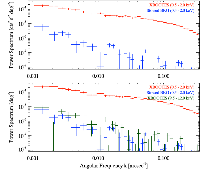
Figure 19: Top: Photon-shot-noise-subtracted power spectra of the total-count map, $\mathbf{C}^{\mathrm{Total}}$ in the terminology of Sect. 2.4, (red crosses) and of the ACIS-I stowed-background map $\mathbf{C}^{\mathrm{Stow}}$ (blue crosses) in the $0.5-2.0\,\mathrm{keV}$ band. Bottom: Same as top panel but in the units of squared fractional RMS power spectrum $Q(k)$ (Eq. 17). Also shown in the bottom panel is the power spectrum for the total-count map $\mathbf{C}^{\mathrm{Total}}$ in the $9.5-12.0\,\mathrm{keV}$ band (green crosses).

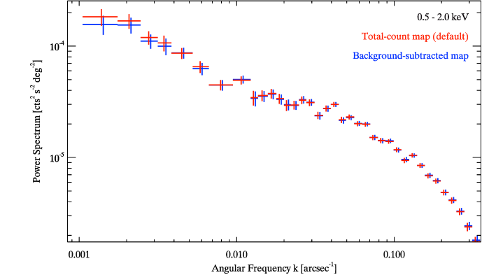
Figure 20: Photon-shot-noise-subtracted power spectrum in the $0.5-2.0\,\mathrm{keV}$ band computed from the total-count map $\mathbf{C}_{X}^{\mathrm{Total}}$ (red) and the background-subtracted map $\mathbf{C}_{X}^{\mathrm{CXB}}$ (blue, Eq. 4, Sect. 2.4).

References

- Aird et al. (2010) Aird J. et al., 2010, MNRAS, 401, 2531
- Alexander & Hickox (2012) Alexander D. M., Hickox R. C., 2012, New A Rev., 56, 93
- Alexander et al. (2013) Alexander D. M. et al., 2013, ApJ, 773, 125
- Allevato et al. (2011) Allevato V. et al., 2011, ApJ, 736, 99
- Allevato et al. (2014) Allevato V. et al., 2014, ApJ, 796, 4
- Allevato et al. (2012) Allevato V. et al., 2012, ApJ, 758, 47
- Anders & Grevesse (1989) Anders E., Grevesse N., 1989, Geochim. Cosmochim. Acta, 53, 197
- Anderson et al. (2015) Anderson M. E., Gaspari M., White S. D. M., Wang W., Dai X., 2015, MNRAS, 449, 3806
- Arnaud (1996) Arnaud K. A., 1996, in Astronomical Society of the Pacific Conference Series, Vol. 101, Astronomical Data Analysis Software and Systems V, Jacoby G. H., Barnes J., eds., p. 17
- Baganoff (1999) Baganoff F., 1999, Acis on-orbit background rates and spectra from chandra oac phase 1. ACIS Memo 162, Massachusetts Institute of Technology, Centerfor Space Research
- Barcons & Fabian (1988) Barcons X., Fabian A. C., 1988, MNRAS, 230, 189
- Blanton et al. (2003) Blanton M. R., Lin H., Lupton R. H., Maley F. M., Young N., Zehavi I., Loveday J., 2003, AJ, 125, 2276
- Böhringer, Chon & Collins (2014) Böhringer H., Chon G., Collins C. A., 2014, A&A, 570, A31
- Brandt & Alexander (2015) Brandt W. N., Alexander D. M., 2015, A&A Rev., 23, 1
- Brandt & Hasinger (2005) Brandt W. N., Hasinger G., 2005, ARA&A, 43, 827
- Brusa et al. (2009) Brusa M. et al., 2009, ApJ, 693, 8
- Cappelluti, Allevato & Finoguenov (2012) Cappelluti N., Allevato V., Finoguenov A., 2012, Advances in Astronomy, 2012, 1
- Cappelluti et al. (2013) Cappelluti N. et al., 2013, ApJ, 769, 68
- Carter et al. (2003) Carter C., Karovska M., Jerius D., Glotfelty K., Beikman S., 2003, in Astronomical Society of the Pacific Conference Series, Vol. 295, Astronomical Data Analysis Software and Systems XII, Payne H. E., Jedrzejewski R. I., Hook R. N., eds., p. 477
- Cheng, Wu & Cooray (2004) Cheng L.-M., Wu X.-P., Cooray A., 2004, A&A, 413, 65
- Clerc et al. (2012) Clerc N., Sadibekova T., Pierre M., Pacaud F., Le Fèvre J.-P., Adami C., Altieri B., Valtchanov I., 2012, MNRAS, 423, 3561
- Comastri et al. (1995) Comastri A., Setti G., Zamorani G., Hasinger G., 1995, A&A, 296, 1
- Cooray & Sheth (2002) Cooray A., Sheth R., 2002, Phys. Rep., 372, 1
- Dawson et al. (2013) Dawson K. S. et al., 2013, AJ, 145, 10
- De Luca & Molendi (2004) De Luca A., Molendi S., 2004, A&A, 419, 837
- Diego et al. (2003) Diego J. M., Sliwa W., Silk J., Barcons X., 2003, MNRAS, 344, 951
- Dodelson (2003) Dodelson S., 2003, Modern cosmology, 1st edn. Academic Press
- Ebeling et al. (1997) Ebeling H., Edge A. C., Fabian A. C., Allen S. W., Crawford C. S., Böhringer H., 1997, ApJ, 479, L101
- Ebeling et al. (1996) Ebeling H., Voges W., Bohringer H., Edge A. C., Huchra J. P., Briel U. G., 1996, MNRAS, 281, 799
- Eisenstein & Hu (1998) Eisenstein D. J., Hu W., 1998, ApJ, 496, 605
- Fabian & Barcons (1992) Fabian A. C., Barcons X., 1992, ARA&A, 30, 429
- Fanidakis et al. (2013) Fanidakis N. et al., 2013, MNRAS, 435, 679
- Finoguenov et al. (2007) Finoguenov A. et al., 2007, ApJS, 172, 182
- Finoguenov et al. (2015) Finoguenov A. et al., 2015, A&A, 576, A130
- Finoguenov et al. (2010) Finoguenov A. et al., 2010, MNRAS, 403, 2063
- Frigo & Johnson (2005) Frigo M., Johnson S. G., 2005, Proceedings of the IEEE, 93, 216, special issue on “Program Generation, Optimization, and Platform Adaptation”
- Fruscione et al. (2006) Fruscione A. et al., 2006, in Society of Photo-Optical Instrumentation Engineers (SPIE) Conference Series, Vol. 6270, Society of Photo-Optical Instrumentation Engineers (SPIE) Conference Series
- Gendreau et al. (1995) Gendreau K. C. et al., 1995, PASJ, 47, L5
- Georgakakis et al. (2008) Georgakakis A., Nandra K., Laird E. S., Aird J., Trichas M., 2008, MNRAS, 388, 1205
- Giacconi (2013) Giacconi R., 2013, Mem. Soc. Astron. Italiana, 84, 472
- Giacconi et al. (1962) Giacconi R., Gursky H., Paolini F. R., Rossi B. B., 1962, Physical Review Letters, 9, 439
- Giles et al. (2015) Giles P. A. et al., 2015, ArXiv e-prints
- Gilli, Comastri & Hasinger (2007) Gilli R., Comastri A., Hasinger G., 2007, A&A, 463, 79
- Hamilton & Helfand (1987) Hamilton T. T., Helfand D. J., 1987, ApJ, 318, 93
- Hasinger, Miyaji & Schmidt (2005) Hasinger G., Miyaji T., Schmidt M., 2005, A&A, 441, 417
- Helgason et al. (2014) Helgason K., Cappelluti N., Hasinger G., Kashlinsky A., Ricotti M., 2014, ApJ, 785, 38
- Henley & Shelton (2013) Henley D. B., Shelton R. L., 2013, ApJ, 773, 92
- Hennawi et al. (2006) Hennawi J. F. et al., 2006, AJ, 131, 1
- Hickox et al. (2009) Hickox R. C. et al., 2009, ApJ, 696, 891
- Hickox & Markevitch (2006) Hickox R. C., Markevitch M., 2006, ApJ, 645, 95
- Hickox & Markevitch (2007) Hickox R. C., Markevitch M., 2007, ApJ, 661, L117
- Hogg (1999) Hogg D. W., 1999, ArXiv Astrophysics e-prints, 9905116
- Hopkins et al. (2006) Hopkins P. F., Hernquist L., Cox T. J., Di Matteo T., Robertson B., Springel V., 2006, ApJS, 163, 1
- Hütsi et al. (2014) Hütsi G., Gilfanov M., Kolodzig A., Sunyaev R., 2014, A&A, 572, A28
- Kalberla et al. (2005) Kalberla P. M. W., Burton W. B., Hartmann D., Arnal E. M., Bajaja E., Morras R., Pöppel W. G. L., 2005, A&A, 440, 775
- Kashlinsky et al. (2005) Kashlinsky A., Arendt R. G., Mather J., Moseley S. H., 2005, Nature, 438, 45
- Kayo & Oguri (2012) Kayo I., Oguri M., 2012, MNRAS, 424, 1363
- Kenter et al. (2005) Kenter A. et al., 2005, ApJS, 161, 9
- Kim et al. (2007) Kim M., Wilkes B. J., Kim D.-W., Green P. J., Barkhouse W. A., Lee M. G., Silverman J. D., Tananbaum H. D., 2007, ApJ, 659, 29
- Kolodzig et al. (2013a) Kolodzig A., Gilfanov M., Hütsi G., Sunyaev R., 2013a, A&A, 558, A90
- Kolodzig et al. (2013b) Kolodzig A., Gilfanov M., Sunyaev R., Sazonov S., Brusa M., 2013b, A&A, 558, A89
- Komatsu & Kitayama (1999) Komatsu E., Kitayama T., 1999, ApJ, 526, L1
- Komatsu et al. (2011) Komatsu E. et al., 2011, ApJS, 192, 18
- Kravtsov & Borgani (2012) Kravtsov A. V., Borgani S., 2012, ARA&A, 50, 353
- Krumpe, Miyaji & Coil (2010) Krumpe M., Miyaji T., Coil A. L., 2010, ApJ, 713, 558
- Krumpe, Miyaji & Coil (2014) Krumpe M., Miyaji T., Coil A. L., 2014, in Multifrequency Behaviour of High Energy Cosmic Sources, pp. 71–78
- Krumpe et al. (2012) Krumpe M., Miyaji T., Coil A. L., Aceves H., 2012, ApJ, 746, 1
- Krumpe et al. (2015) Krumpe M., Miyaji T., Husemann B., Fanidakis N., Coil A. L., Aceves H., 2015, ApJ, 815, 21
- LaMassa et al. (2016) LaMassa S. M. et al., 2016, ApJ, 817, 172
- Leauthaud et al. (2015) Leauthaud A. et al., 2015, MNRAS, 446, 1874
- Lehmer et al. (2012) Lehmer B. D. et al., 2012, ApJ, 752, 46
- Lumb et al. (2002) Lumb D. H., Warwick R. S., Page M., De Luca A., 2002, A&A, 389, 93
- Merloni et al. (2012) Merloni A. et al., 2012, ArXiv e-prints, 1209.3114
- Miyaji & Griffiths (2002) Miyaji T., Griffiths R. E., 2002, ApJ, 564, L5
- Miyaji et al. (2015) Miyaji T. et al., 2015, ArXiv e-prints
- Miyaji et al. (2011) Miyaji T., Krumpe M., Coil A. L., Aceves H., 2011, ApJ, 726, 83
- Moretti et al. (2003) Moretti A., Campana S., Lazzati D., Tagliaferri G., 2003, ApJ, 588, 696
- Moretti et al. (2012) Moretti A., Vattakunnel S., Tozzi P., Salvaterra R., Severgnini P., Fugazza D., Haardt F., Gilli R., 2012, A&A, 548, A87
- Mountrichas et al. (2013) Mountrichas G. et al., 2013, MNRAS, 430, 661
- Murray et al. (2005) Murray S. S. et al., 2005, ApJS, 161, 1
- Pacaud et al. (2016) Pacaud F. et al., 2016, A&A, 592, A2
- Pierre et al. (2011) Pierre M., Pacaud F., Juin J. B., Melin J. B., Valageas P., Clerc N., Corasaniti P. S., 2011, MNRAS, 414, 1732
- Planck Collaboration et al. (2015) Planck Collaboration et al., 2015, ArXiv e-prints
- Predehl et al. (2010) Predehl P. et al., 2010, in Society of Photo-Optical Instrumentation Engineers (SPIE) Conference Series, Vol. 7732, Society of Photo-Optical Instrumentation Engineers (SPIE) Conference Series
- Reynolds et al. (2014) Reynolds M. T., Reis R. C., Miller J. M., Cackett E. M., Degenaar N., 2014, MNRAS, 441, 3656
- Richardson et al. (2013) Richardson J., Chatterjee S., Zheng Z., Myers A. D., Hickox R., 2013, ApJ, 774, 143
- Richardson et al. (2012) Richardson J., Zheng Z., Chatterjee S., Nagai D., Shen Y., 2012, ApJ, 755, 30
- Roncarelli et al. (2012) Roncarelli M., Cappelluti N., Borgani S., Branchini E., Moscardini L., 2012, MNRAS, 424, 1012
- Roncarelli et al. (2007) Roncarelli M., Moscardini L., Borgani S., Dolag K., 2007, MNRAS, 378, 1259
- Roncarelli et al. (2006) Roncarelli M., Moscardini L., Tozzi P., Borgani S., Cheng L. M., Diaferio A., Dolag K., Murante G., 2006, MNRAS, 368, 74
- Rosati, Borgani & Norman (2002) Rosati P., Borgani S., Norman C., 2002, ARA&A, 40, 539
- Scheuer (1974) Scheuer P. A. G., 1974, MNRAS, 166, 329
- Shafer & Fabian (1983) Shafer R. A., Fabian A. C., 1983, in IAU Symposium, Vol. 104, Early Evolution of the Universe and its Present Structure, Abell G. O., Chincarini G., eds., pp. 333–342
- Shen et al. (2013) Shen Y. et al., 2013, ApJ, 778, 98
- Sheth, Mo & Tormen (2001) Sheth R. K., Mo H. J., Tormen G., 2001, MNRAS, 323, 1
- Soltan & Hasinger (1994) Soltan A., Hasinger G., 1994, A&A, 288, 77
- Tanaka (2013) Tanaka Y., 2013, Mem. Soc. Astron. Italiana, 84, 485
- Ueda et al. (2014) Ueda Y., Akiyama M., Hasinger G., Miyaji T., Watson M. G., 2014, ApJ, 786, 104
- Ursino et al. (2011) Ursino E., Branchini E., Galeazzi M., Marulli F., Moscardini L., Piro L., Roncarelli M., Takei Y., 2011, MNRAS, 414, 2970
- Ursino, Galeazzi & Huffenberger (2014) Ursino E., Galeazzi M., Huffenberger K., 2014, ApJ, 789, 55
- Vajgel et al. (2014) Vajgel B., Jones C., Lopes P. A. A., Forman W. R., Murray S. S., Goulding A., Andrade-Santos F., 2014, ApJ, 794, 88
- van der Klis (1989) van der Klis M., 1989, in NATO Advanced Science Institutes (ASI) Series C, Vol. 262, NATO Advanced Science Institutes (ASI) Series C, Ögelman H., van den Heuvel E. P. J., eds., p. 27
- Vikhlinin & Forman (1995) Vikhlinin A., Forman W., 1995, ApJ, 455, L109
- Yang et al. (2015) Yang Q.-X., Xie F.-G., Yuan F., Zdziarski A. A., Gierliński M., Ho L. C., Yu Z., 2015, MNRAS, 447, 1692