The RAVE-on catalog of stellar atmospheric parameters and
chemical abundances for chemo-dynamic studies in the Gaia era

Abstract

The orbits, atmospheric parameters, chemical abundances, and ages of individual stars in the Milky Way provide the most comprehensive illustration of galaxy formation available. The Tycho-Gaia Astrometric Solution (TGAS) will deliver astrometric parameters for the largest ever sample of Milky Way stars, though its full potential cannot be realized without the addition of complementary spectroscopy. Among existing spectroscopic surveys, the RAdial Velocity Experiment (RAVE) has the largest overlap with TGAS ($\gtrsim$200,000 stars). We present a data-driven re-analysis of 520,781 RAVE spectra using The Cannon. For red giants, we build our model using high-fidelity APOGEE stellar parameters and abundances for stars that overlap with RAVE. For main-sequence and sub-giant stars, our model uses stellar parameters from the K2/EPIC. We derive and validate effective temperature $T_{\mathrm{eff}}$, surface gravity $\log g$, and chemical abundances of up to seven elements (O, Mg, Al, Si, Ca, Fe, Ni). We report a total of 1,685,851 elemental abundances with a typical precision of 0.07 dex, a substantial improvement over previous RAVE data releases. The synthesis of RAVE-on and TGAS is the most powerful data set for chemo-dynamic analyses of the Milky Way ever produced.

1 Introduction

The Milky Way is considered to be our best laboratory for understanding galaxy formation and evolution. This premise hinges on the ability to precisely measure the astrometry and chemistry for (many) individual stars, and to use those data to infer the structure, kinematics, and chemical enrichment of the Galaxy (e.g., Nordström et al., 2004; Schlaufman et al., 2009; Deason et al., 2011; Casagrande et al., 2011; Ness et al., 2012, 2013a, 2013b; Casey et al., 2012, 2013, 2014a, 2014b; Boeche et al., 2013; Kordopatis et al., 2015; Bovy et al., 2016). However, these quantities are not known for even 1% of stars in the Milky Way. Stellar distances are famously imprecise (e.g., van Leeuwen, 2007; Jofré et al., 2015; Mädler et al., 2016), proper motions can be plagued by unquantified systematics from the first epoch observations (e.g., Casey & Schlaufman, 2015), and stellar spectroscopists frequently report significantly different chemical abundance patterns from the same spectrum (Smiljanic et al., 2014). The impact these issues have on scientific inferences cannot be understated. Imperfect astrometry or chemistry limits understanding in a number of sub-fields in astrophysics, including the properties of exoplanet host stars, the formation (and destruction) of star clusters, as well as studies of stellar populations and Galactic structure, to name a few.

The Gaia mission represents a critical step forward in understanding the Galaxy. Gaia is primarily an astrometric mission, and will provide precise positions, parallaxes and proper motions for more than $10^{9}$ stars in its final data release in 2022. While this is a sample size about four orders of magnitude larger than its predecessor Hipparcos, both astrometry and chemistry are required to fully characterize the formation and evolution of the Milky Way. Gaia will also provide radial velocities, stellar parameters and chemical abundances for a subset of brighter stars, but these measurements will not be available in the first few data releases. Until those abundances are available, astronomers seeking to simultaneously use chemical and dynamical information are reliant on ground-based spectroscopic surveys to complement the available Gaia astrometry.

The first Gaia data release will include the Tycho-Gaia Astrometric Solution (hereafter TGAS; Michalik et al., 2015a, b): positions, proper motions, and parallaxes for approximately two million stars in the Tycho-2 (Høg et al., 2000) catalog. After cross-matching all major stellar spectroscopic surveys, we found that the RAdial Velocity Experiment (RAVE; Steinmetz et al., 2006) survey is expected to have the largest overlap with the first Gaia data release: up to 264,276 stars. We used the Gaia universe model snapshot (Robin et al., 2012) to estimate the precision in parallax and proper motions that could be available in the first Gaia data release (DR1) for stars in those overlap samples. Comparing the expected precision to what is currently available, we further found that the RAVE survey will benefit most from Gaia DR1: the distances of 63% of stars in the RAVE–Gaia DR1 overlap sample are expected to improve with the first Gaia data release, and 47% of stars are likely to have better proper motions. Although the Gaia universe model assumes end-of-mission uncertainties — and does not account for systematics in the first data release — this calculation still provides intuition for the relative improvement that the first Gaia data release can make to ground-based surveys. The expected improvements for RAVE motivated us to examine what chemical abundances were available from those data, and to evaluate whether we could enable new chemo-dynamic studies by contributing to the existing set of chemical abundances.

We briefly describe the RAVE data in Section 2, before explaining our methods in Section 3. In Section 4 we outline a number of validation experiments, including: internal sanity checks, comparisons with literature samples, and investigations to ensure our results are consistent with expectations from astrophysics. We discuss the implications of these comparisons in Section 5, and conclude with instructions on how to access our results electronically.

2 Data

RAVE is a magnitude-limited stellar spectroscopic survey of the (nearby) Milky Way, principally designed to measure radial velocities for up to $10^{6}$ stars. Observations were conducted on the 1.2 m UK Schmidt telescope at the Australian Astronomical Observatory from 2003–2013. A large 5.7 degree field-of-view and robotic fibre positioner made for very efficient observing: spectra for up to 150 targets could be simultaneously acquired. When observations concluded in April 2013, at least 520,781 useful spectra had been collected of more than 457,588 unique objects.

The target selection for RAVE is based on the $I$-band apparent magnitude, $9<I<12$, with a weak $J-K_{s}>0.5$ cut near the disk and bulge (Wojno et al., 2016). The $I$ band was used for the target selection because it has a good overlap with the wavelength range that RAVE operates in: 8410–8795 Å. The resolution and wavelength coverage of RAVE is comparable to the Radial Velocity Spectrometer on board the Gaia space telescope (Munari et al., 2005; Kordopatis et al., 2011; Recio-Blanco et al., 2016), and the wavelength range overlaps with one of the key setups used for the ground-based high-resolution Gaia-ESO survey (Gilmore et al., 2012; Randich et al., 2013). The spectral region includes the Ca II near infrared triplet lines — strong transitions that are dominated by pressure broadening — which are visible even in metal-poor stars or spectra with very low signal-to-noise (S/N) ratios. Atomic transitions of light-, $\alpha$-, and Fe-peak elements are also present, allowing for detailed chemical abundance studies.

The exposure times for RAVE observations were optimised to obtain radial velocities for as many stars as possible. Detailed chemical abundances were always an important science goal of the survey, but this was a secondary objective. For this reason the distribution of S/N ratios in RAVE spectra is considerably lower than other stellar spectroscopic surveys where chemical abundances are the primary motivation. The RAVE spectra have an effective resolution $\mathcal{R}\approx 7{,}500$ and the distribution of S/N ratios peaks at $\approx$50 pixel^-1. For comparison, the GALAH survey (De Silva et al., 2015) — which was specifically constructed for detailed chemical abundance analyses — includes a wavelength range about 2.5 times larger at resolution $\mathcal{R}\approx 28{,}000$, and yet the GALAH project still targets for S/N $\gtrsim 100$ per resolution element.

Despite the relatively low resolution and S/N of the spectra compared to other surveys, the RAVE data releases have provided excellent radial velocities, stellar atmospheric parameters ($T_{\mathrm{eff}}$, $\log g$), and detailed chemical abundances (Steinmetz et al., 2006; Zwitter et al., 2008; Siebert et al., 2011; Boeche et al., 2011; Kordopatis et al., 2013; Kunder et al., 2016). In this work we make use of spectra that has been reprocessed for the fifth RAVE data release. These re-processing steps include: a detailed re-reduction of all the original data frames, with flux variances propagated at every step; an updated continuum-normalization procedure; as well as revised determinations of stellar radial velocities and morphological classifications. At the end of this processing for each survey observation we were provided with: rest-frame wavelengths (without resampling), continuum-normalized fluxes, $1\sigma$ uncertainties in the continuum-normalized flux values, as well as relevant metadata for each observation. We refer the reader to the official fifth data release paper of the RAVE survey, as presented by Kunder et al. (2016), for more details of this re-processing.

Given the high-quality of the normalization performed by the RAVE team, we chose not to re-normalize the spectra. Our tests demonstrated that the procedure outlined in Kunder et al. (2016) is sufficient for our analysis procedure. Therefore, there were a limited number of pre-processing steps that we performed before starting our analysis. First, we calculated inverse variance arrays from the $1\sigma$ uncertainties provided, and then we re-sampled the flux and inverse variance arrays onto a common rest-wavelength map for all stars. Depending on the fibre used and the stellar radial velocity, the range of rest-frame wavelength values varied for each star. Given that fluxes were unavailable in the edge pixels for most stars, we excluded pixels outside of the rest wavelength range $8423.2\,{\rm\AA}\leq\lambda\leq 8777.6\,{\rm\AA}$. This corresponds to about 30 pixels excluded on either side of the common wavelength array, leaving us with 945 pixels per spectrum for science.

3 Method

We chose to adopt a data-driven model for this analysis, in contrast to the physics-based models used in RAVE data releases to date. Specifically, we will use an implementation of The Cannon (Ness et al., 2015, 2016). Although this choice complicated the construction of our model (e.g., see Section 3.2), a data-driven approach makes use of all available information in the spectrum and lowers the S/N ratio at which systematic effects begin to dominate. In other words, in the low S/N regime, a well-constructed data-driven model will yield more precise labels (e.g., stellar parameters and chemical abundances) than most physics-driven models. This is particularly relevant for the low-resolution RAVE data analysed here, because about half of the spectra have S/N $\lesssim 50$ pixel^-1.

There are two main analysis steps when using The Cannon: the training step and the test step. We describe these stages in the context of our model in the following section, and a more thorough introduction can be found in Ness et al. (2015). We make the following explicit assumptions about the RAVE spectra and The Cannon:

• We assume that any fibre- and time-dependent variations in spectral resolution in the RAVE spectra are negligible.

• The RAVE noise variances are approximately correct, independent between pixels, and normally distributed.

• We assume that the normalization procedure employed by the RAVE pipeline is invariant with respect to the labels we seek to measure (e.g., $T_{\mathrm{eff}}$, $\log g$, or [Fe/H]), and invariant with respect to the S/N ratio. In other words, we assume that the normalization procedure does not produce different results for high S/N spectra compared to low S/N spectra, nor does the normalization procedure vary non-linearly with respect to stellar parameters (e.g., [Fe/H]).

• We assume that stars with similar labels ($T_{\mathrm{eff}}$, $\log g$, and abundances) have similar spectra.

• A stellar spectrum is a smooth function of the label values for that star, and we assume that the function is smooth enough within a sub-space of the labels (e.g., the giant branch or the main-sequence) that it can be reasonably approximated with a low-order polynomial in label space.

• The training set (Section 3.2) has mean accurate labels for most, but not all stars. That is to say that we do not assume that every label in the training is accurate. We can afford to have a small fraction of inaccurate labels; a few obvious misclassifications in the training set are affordable.

• We assume that the training data are similar (in spectra) to the test data where they overlap in label space, and we assume that the training data spans enough of the label space to capture the variation in the test-set spectra.

3.1 The model

Given our assumptions, the model we adopt is

$$y_{jn} = \bm{v}(\ell_{n})\cdot\bm{\theta}_{j}+e_{jn}\quad,$$ (1)

where $y_{jn}$ is the pseudo-continuum-normalized flux for star $n$ at wavelength pixel $j$, $\bm{v}(\ell_{n})$ is the vectorizing function that takes as input the $K$ labels $\ell_{n}$ for star $n$ and outputs functions of those labels as a vector of length $D>K$, $\bm{\theta}_{j}$ is a vector of length $D$ of parameters influencing the model at wavelength pixel $j$, and $e_{jn}$ is the residual (noise). Here we will only consider vectorizing functions with second-order polynomial expansions (e.g., $T_{\mathrm{eff}}^{2}$, see Sections 3.3–3.5). The noise values $e_{jn}$ can be considered to be drawn from a Gaussian distribution with zero mean and variance $\sigma_{jn}^{2}+s_{j}^{2}$, where $\sigma_{jn}^{2}$ is the variance in flux $y_{jn}$ and $s_{j}^{2}$ describes the excess variance at the $j$-th wavelength pixel.

At the training step we fix the $K$-lists of labels for the $n$ training set stars. At each wavelength pixel $j$, we then find the parameters $\bm{\theta}_{j}$ and $s_{j}^{2}$ by optimizing the penalized likelihood function

$$\bm{\theta}_{j},s^{2}_{j} \leftarrow \underset{\bm{\theta},s}{\operatorname{argmin}}\,\left[\sum_{n=0}^{N-1}\frac{[y_{jn}-\bm{v}(\ell_{n})\cdot\bm{\theta}]^{2}}{\sigma^{2}_{jn}+s^{2}}+\sum_{n=0}^{N-1}\ln(\sigma^{2}_{jn}+s^{2})+\Lambda{}\,Q(\bm{\theta})\right]\quad,$$ (2)

where $\Lambda$ is a regularization parameter which we will heuristically set in later sections, and $Q(\bm{\theta})$ is a L1 regularizing function that encourages $\bm{\theta}$ values to take on zero values without breaking convexity (Casey et al., 2016):

$$Q(\bm{\theta})=\sum_{d=1}^{D-1}|{\theta_{d}}|\quad.$$ (3)

Note that the $d$ subscript here is zero-indexed; the function $Q(\bm{\theta})$ does not act on the (first) $\theta_{0}$ coefficient, as this is a ‘pivot point’ (mean flux value) that we do not expect to diminish with increasing regularization (e.g., see equation 5). In practice we first fix $s_{j}^{2}=0$ to make equation 2 a convex optimization problem, then we optimize for $\bm{\theta}_{j}$, before solving for $s_{j}^{2}$.

The test step is where we fix the parameters $\bm{\theta}_{j},s_{j}^{2}$ at all wavelength pixels $j$, and optimize the $K$-list of labels $\ell_{m}$ for the $m$-th test set star. Here the objective function is:

$$\ell_{m} \leftarrow \underset{\ell}{\operatorname{argmin}}\,\left[\sum_{j=0}^{J-1}\frac{[y_{jm}-\bm{v}(\ell)\cdot\bm{\theta}_{j}]^{2}}{\sigma_{jm}^{2}+s_{j}^{2}}\right]\quad.$$ (4)

After optimizing equation 4 for the $m$-th star we store the covariance matrix $\bm{\Sigma}_{m}$ for the labels $\ell_{m}$, which provides us with the formal errors on $\ell_{m}$. The formal errors are expected to be underestimated, and in Section 4 we judge the veracity of these errors through validation experiments.

3.2 The training set

We sought to construct a training set of stars across the main-sequence, the sub-giant branch, and the red giant branch. We required stars with precisely measured effective temperature $T_{\mathrm{eff}}$, surface gravity $\log g$, and elemental abundances of O, Mg, Si, Ca, Al, Fe, and Ni. This proved to be difficult because the magnitude range of RAVE does not overlap substantially with high-resolution spectroscopic surveys. The fourth internal data release of the Gaia-ESO survey includes giant and main-sequence stars, but only 142 overlap with RAVE, which is too small to be a useful training set for our purposes. The thirteenth data release from the Sloan Digital Sky Survey (SDSS Collaboration et al., 2016) includes labels for APOGEE stars on the giant branch and (uncalibrated values for) the main-sequence, but our tests indicated that the APOGEE main-sequence labels suffered from significant systematic effects. A flat, then ‘up-turning’ main-sequence is present, and the metallicity gradient trends in the opposite direction with respect to $\log g$ on the main-sequence (i.e., metal-poor stars incorrectly sit above an isochrone in a classical Hertzsprung-Russell diagram). If we consider lower-resolution studies as potential training sets, there are 2,369 stars that overlap with LAMOST — of which 2,213 have positive S/N ratios in the $g$-band (snrg). However, the labels are expectedly less precise given the lower resolution, there are no elemental abundances available for the main-sequence stars, and the LAMOST lower main-sequence suffers from the same systematic effects seen in the APOGEE data.

These constraints forced us to construct a heterogeneous training set. Given previous successes in transferring high S/N ratio labels from APOGEE (Ness et al., 2015, 2016; Ho et al., 2016; Casey et al., 2016), we chose to use the 1,355 stars in the APOGEE—RAVE overlap sample for giant star labels in the training set. Of these, about 900 are giants according to APOGEE. From this sample we selected stars to have: determinations in all abundances of interest ([X/H] $>-5$ for O, Mg, Al, Si, Ca, Fe, and Ni); S/N ratios of $>$200 pixel^-1 in APOGEE and $>$25 pixel^-1 in RAVE; and we further required that the ASPCAP did not report any peculiar flags (ASPCAPFLAG = 0). These restrictions left us with 536 stars along the giant branch, with metallicities ranging from $[{\rm Fe/H}]=-1.79$ to 0.26. Intermediate tests with globular cluster members showed that the metallicity range of the training set needed to extend at least below $[{\rm Fe/H}]\lesssim-2$ in order for our catalog to be practically useful. Without additional metal-poor stars, the lowest metallicity labels reported by our model would be around $[{\rm Fe/H}]\approx-2$, even for well studied stars with $[{\rm Fe/H}]\sim-4$ (e.g., CD 38-245). For this reason we supplemented our sample of APOGEE giant stars with 176 known metal-poor giant stars observed by RAVE. The effective temperature $T_{\mathrm{eff}}$, surface gravity $\log g$ and iron abundance [Fe/H] labels were adopted from Fulbright et al. (2010); Ruchti et al. (2011). For this sample of metal-poor stars, we assumed that the elemental abundances of O, Mg, Al, Si, Ca, and Ni followed typical trends of Galactic chemical evolution: we asserted $[{\rm Mg/Fe}]=+0.4$, $[{\rm O/Fe}]=+0.4$, $[{\rm Al/Fe}]=-0.5$, $[{\rm Ca/Fe}]=+0.4$, $[{\rm Si/Fe}]=+0.4$, and $[{\rm Ni/Fe}]=-0.25$. We stress that this decision is made solely to ensure that our overall metallicity scale reflects that of the RAVE survey, down to $[{\rm Fe/H}]\sim-4$. Indeed, it is likely that for most of these elements, these abundances cannot be measured from RAVE spectra for ultra metal-poor stars: the atomic transitions in the RAVE spectral region are simply too weak to influence the spectrum. For this reason, our adopted abundances for these very metal-poor stars represent an ‘anchor point’ in order to ensure our overall metallicity scale is correct. We do not recommend the use of our individual abundance labels at $[{\rm Fe/H}]\sim-4$. We discuss this issue in more detail in Section 5.

Assembling a suitable training set for the main-sequence and sub-giant branch was less trivial. There are no spectroscopic studies that extend the range of stellar types we are interested in (e.g., FGKM-type stars), and which also have a large enough sample size that overlaps with RAVE. Moreover, most of the spectroscopic studies we considered also showed a flat lower main-sequence, a systematic consequence of the analysis method adopted (see Bensby et al., 2014, for discussion on this issue). For these reasons we chose to make use of the K2/EPIC catalog (Huber et al., 2016) for the training set labels on the main-sequence and sub-giant branch. The K2/EPIC catalog follows from the successful Kepler input catalog (Brown et al., 2011), and provides probabilistic stellar classifications for 138,600 stars in the K2 fields based on the astrometric, asteroseismic, photometric, and spectroscopic information available for every star. There are 4,611 stars that overlap between K2/EPIC and RAVE.

K2/EPIC differs from the Kepler input catalog because K2/EPIC does not benefit from having narrow-band $DDO_{51}$ photometry to aid dwarf/giant classification. Despite this limitation, the labels in the K2/EPIC catalog have already been shown to be accurate and trustworthy (Huber et al., 2016). However, when the posteriors are wide (i.e., the quoted confidence intervals are large) due to limited information available, it is possible that a star has been misclassified. This is most prevalent for sub-giants, where Huber et al. (2016) note that $\approx 55-70$% of sub-giants are misclassified as dwarfs. The probability of misclassification is usually quantified in the uncertainties given for each star; most dwarfs that have a higher possibility of being sub-giants have large confidence intervals. Therefore, requiring low uncertainties will decrease the total sample size, but in practice it removes most misclassifications. The situation is far more favourable for dwarfs and giants. Only 1–4% of giant stars are misclassified as dwarfs, and about 7% of dwarfs are misclassified as giants. To summarise, the K2/EPIC labels with narrow confidence intervals are usually of high fidelity, and given that we have spectra, we can identify any obvious misclassifications.

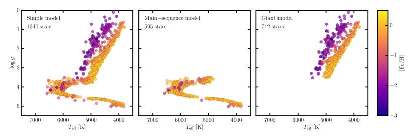
Figure 1: Effective temperature $T_{\mathrm{eff}}$ and surface gravity $\log g$ for all stars in the training sets. Stars are colored by their metallicity [Fe/H], and the three panels show stars in the simple model (left panel; Section 3.3), the main-sequence star model (middle panel; Section 3.4), and the giant star model (right panel; Section 3.5).

We sought to have a small overlap between our giant and main-sequence star training sets. Most of our giant training set is encapsulated within $0<\log g<3.5$, however there is a sparse sampling of stars reaching to $\log g\approx 4$. We required $\log g>3.5$ for the K2/EPIC main-sequence/sub-giant star training set, allowing for $\approx 0.5$ dex of overlap between the two training sets. We further employed the following quality constraints on the K2/EPIC catalog: the upper and lower confidence intervals in $T_{\mathrm{eff}}$ must be below 150 K; the upper and lower confidence intervals in $\log g$ must be less than 0.15 dex; the S/N of the RAVE spectra must exceed 30 pixel^-1; and $T_{\mathrm{eff}}\leqslant 6750$ K. Unfortunately these strict constraints removed most metal-poor stars, which we later found to cause the test labels to have under-predicted abundances for dwarfs of low metallicity. For this reason we relaxed (ignored) those quality constraints for stars with $[{\rm Fe/H}]<-1$, and included an additional 12 turn-off stars with $-1.6\gtrsim[{\rm Fe/H}]\gtrsim-2.1$ from Ruchti et al. (2011). After training a model based on main-sequence and giant stars (Section 3.1), we found we could identify misclassifications by leave-one-out cross-validation. However, we chose not to do this because the number of likely misclassifications in the training set was negligible ($\approx$1%), and the improvement in main-sequence test set labels was minimal. The distilled sample of the RAVE–K2/EPIC overlap catalog contains 595 stars (583 of 4,611 from K2/EPIC). The full training set for each model (see next sections) is shown in Figure 1.

3.3 The simple model: a 3-label model ($T_{\mathrm{eff}}$, $\log g$, $[\mathrm{Fe/H}]$) for all stars

We have constructed a justified training set for stars across the main-sequence, sub-giant, and red giant branch. However the lack of overlap between RAVE and other works have resulted in a somewhat peculiar situation. Detailed abundances are available from APOGEE for all giant stars in our sample, however only imprecise (but accurate on expectation) metallicities are available from K2/EPIC for stars on the main-sequence and the sub-giant branch. Here we will construct a simple model for all stars that only makes use of three labels ($T_{\mathrm{eff}}$, $\log g$, [Fe/H]), before we outline how we derive abundances for giant branch stars. The complexity for this model will be quadratic ($T_{\mathrm{eff}}^{2}$ is the highest term), where the vectorizer $\bm{v}(\ell_{n})$ expands as,

$$\bm{v}(\ell_{n})\rightarrow\left[1,T_{{\rm eff},n},\log g_{n},[{\rm Fe/H}]_{n},T_{{\rm eff},n}^{2},\log g_{n}\,T_{{\rm eff},n},[\mathrm{Fe/H}]_{n}\,T_{{\rm eff},n},\log g_{n}^{2},[\mathrm{Fe/H}]_{n}\,\log g_{n},[\mathrm{Fe/H}]_{n}^{2}\right]$$ (5)

such that $\bm{v}(\ell)$ produces the design matrix:

$$\bm{v}(\ell)\rightarrow\begin{bmatrix}\bm{v}(\ell_{0})\\ \vdots\\ \bm{v}(\ell_{N-1})\end{bmatrix}\quad.$$ (6)

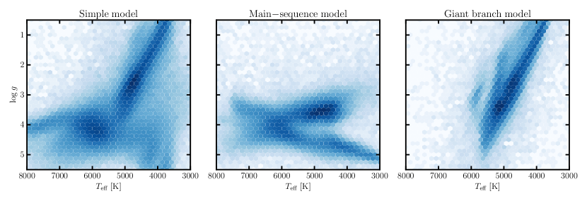
Figure 2: The logarithmic density of effective temperature $T_{\mathrm{eff}}$ and surface gravity $\log g$ for all 520,781 RAVE spectra, as derived using the simple model (left panel; Section 3.3), the main-sequence star model (center panel; Section 3.4), and the giant star model (right panel; Section 3.5). These panels demonstrate how a single quadratic model is insufficient for all RAVE stars (left panel), and illustrate some of the systematic artefacts that can result from testing on stars outside of the training set (center and right panel). These panels do not represent our final results, which are shown in Figure 6.

We used no regularization ($\Lambda=0$) for this model. After training the model we treated all 520,781 spectra as test set objects. In the left-hand panel of Figure 2 we show the effective temperature $T_{\mathrm{eff}}$ and surface gravity $\log g$ for all spectra. The main-sequence and red giant branch are clearly visible. However, the details of stellar evolution are no longer present: the sub-giant branch is not discernible, and there are a number of systematic artefacts (over-densities) present in label space. These artefacts disappear when we require additional quality constraints (e.g., no peculiar morphological classifications), but the complexity of the Hertzsprung-Russell diagram is still not present. Thus, we concluded that while this model could be useful for deriving stellar classifications (e.g., F2-type giant), the labels are too imprecise.

We chose to adopt separate models for the main-sequence and the red giant branch rather than switch to a single model with higher complexity. This choice allowed us to derive stellar parameters for stars on the main-sequence and sub-giant branch, as well as detailed elemental abundances for red giant branch stars. However, adopting two separate models introduces the challenge of how to combine the results from two models, or how to assign one star as ‘belonging’ to a single model. In Section 3.6 we describe how we will use the simple model introduced in this section to discriminate between results from a 3-label main-sequence model in Section 3.4 and a 9-label giant star model in Section 3.5.

3.4 A 3-label model ($T_{\mathrm{eff}}$, $\log g$, $[\mathrm{Fe/H}]$) for unevolved stars

We constructed a three-label quadratic model using only main-sequence and sub-giant stars. In order to set the regularization hyperparameter $\Lambda$ for this model, we trained 30 models with different regularization strengths, spaced evenly in logarithmic steps between $\Lambda=10^{-3}$ to $\Lambda=10^{3}$. We then performed leave-one-out cross-validation for each model. Specifically, for each star in the training set: we removed the star; trained the model; and then inferred labels from the removed star as if it was a test object. We also performed leave-one-out cross-validation on an unregularized ($\Lambda=0$) model, which we will use as the basis for comparison. For the unregularized case, we calculated the bias and root-mean-square (RMS) deviation between: the training set labels, and the labels we derived by cross-validation, where one star was removed at a time and the model was re-trained. We repeated this calculation of bias and RMS deviation for all 30 models with different regularization strengths $\Lambda$.

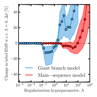
Figure 3: The percentage change in RMS deviation between inferred and training labels at different regularization strengths. The RMS values were calculated by leave-one-out cross-validation, and are shown with respect to an unregularized model ($\Lambda=0$). The points and solid line indicate the mean improvement across all labels. The filled area represents the minimum and maximum improvements over all labels. With increasing regularization strength, there is a minimum in the RMS deviation over all labels, which is where we set $\Lambda$ for each model (see text for details).

We show the percentage difference in the RMS deviation of the labels with respect to the unregularized model in Figure 3. The upper and lower envelope represent the boundaries across all labels, showing that with increasing regularization, the RMS decreased in all labels. We found similar improvements in the biases, however these were already minimal in the unregularized case. The improvement in RMS reaches a minimum value near $\Lambda=35.6$ ($\approx 10^{1.5}$), where we achieve RMS deviations that are about 10% better than the unregularized case. Based on this improvement we set $\Lambda=35.6$ for this model. At this regularization strength, the bias and RMS values found by leave-one-out cross validation are, respectively: $38$ K and $256$ K for $T_{\mathrm{eff}}$, $0.05$ dex and $0.29$ dex for $\log g$, with $0.03$ dex and $0.17$ dex for [Fe/H].

We inferred labels for all 520,781 RAVE spectra using this main-sequence/sub-giant star model; we made no a priori decisions as to whether a star was likely a main-sequence/sub-giant star or not. The results for the entire survey sample are shown in the center panel of Figure 2. The increased density of solar-type stars is consistent with RAVE observing stars in the local neighbourhood, and the high number of turn-off and main-sequence stars relative to the sub-giant branch is expected from the relative lifetimes of these evolutionary phases. An over-density of stars near the base of the giant branch is also present. This artefact is due to having giant stars in the test set, but not in the training set, and the model is (poorly) extrapolating outside the convex hull of the training set.

3.5 A 9-label model for detailed abundances of giant stars

The red giant branch stars in our training set have stellar parameters ($T_{\mathrm{eff}}$, $\log g$) and up to 15 elemental abundances from the ASPCAP (García Pérez et al., 2016). A subset of these elements have atomic transitions in the RAVE wavelength region: O I, Mg I, Al I, Si I, Ca II, Ti I, Fe I, and Ni I. However, we excluded [Ti/H] from our abundance list because of systematics in the ASPCAP [Ti/H] abundances (Holtzman et al., 2015; Hawkins et al., 2016). Therefore we are left with nine labels in our giant star model: $T_{\mathrm{eff}}$, $\log g$, and seven elemental abundances.

Similar to Sections 3.3 and 3.4, we used a quadratic vectorizer for the giant star model. Here the terms are expanded in the same way as equation 5, only with nine labels instead of three. We set the regularization hyperparameter $\Lambda$ in the same way described in Section 3.4, using the same 30 trials of $\Lambda$. The results are shown in Figure 3, where again the enveloped region represents the minimum and maximum change in RMS label deviation with respect to the unregularized case. At the point of maximum improvement near $\Lambda=0.13$ $(\approx 10^{-0.9})$, the RMS in all nine labels has decreased by up to $30$%, with all labels showing an improvement $>5$%, and the mean improvement over all labels is about 10%. Near $\Lambda\approx 10^{-0.9}$ to $10^{-0.3}$, the regularization also produces a sparser matrix of $\bm{\theta}$, with $\approx 20$% more terms (mostly cross-terms) having zero-valued entries. Based on the increased model sparsity and decreasing RMS deviation in the labels, we adopt $\Lambda=0.57$ ($10^{-0.25}$) for the giant star model. The bias in labels from a regularized model with $\Lambda=0.57$ is negligible: $-0.3$ K in $T_{\mathrm{eff}}$, and $<$0.007 dex in magnitude for $\log g$ and all seven elemental abundances. The RMS at this regularization strength is 69 K in $T_{\mathrm{eff}}$, 0.18 dex in $\log g$, and varies between $0.07-0.09$ dex depending on the elemental abundance.

We inferred labels for all 520,781 RAVE spectra using this model, again without regard for whether a star was likely a giant or not. The results for all survey stars are summarized in the right panel of Figure 2. The red clump is clearly visible and in the expected location, without requiring any post-analysis calibration. However, artefacts due to dwarf stars being present in the test set, and not in the training set, are also present.

3.6 Deriving joint estimates from multiple models

We have derived labels for all 520,781 RAVE spectra using the three models described in previous sections. The results from our first model (Section 3.3) — which includes the main-sequence, sub-giant and red giant branch — shows that a single 3-label quadratic model is too simple for the RAVE spectral range. The other models have problems, too: unrealistic over-densities in label space show that the main-sequence model and the giant model make very poor extrapolations for stars outside their respective training sets. For these reasons we were forced to exclude or severely penalize incorrect results from both models. We emphasize that the choices here are entirely heuristic, and depart from interpreting The Cannon output labels as the maxima of individual likelihood functions. Each model produces estimates of the labels for a given star, and we use those estimates to produce a unified estimate, but this joint estimate is calculated by disregarding the probabilistic attributes of individual estimates.

Before attempting to join the results from the models in Sections 3.4 and 3.5, we excluded results in either model that had a reduced $\chi_{r}^{2}>3$. We further discarded stars with labels that are outside the extent of the training set. Specifically for the results from the giant model we (conservatively) excluded stars with derived $\log g>3.5$, and for the results from the main-sequence model we excluded sub-giant stars ($\log g<4$ and $T_{\mathrm{eff}}<5000$ K) that were outside the two-dimensional ($T_{\mathrm{eff}}$, $\log g$) convex hull of the training set used for the main-sequence model. Unfortunately these restrictions did not remove all spurious results. The reason for this can be explained with an example: consider that our giant star model was trained with only giant stars but tested with both giant stars and dwarf stars. Some classes of stars (e.g., metal-poor dwarfs) can project into a region of label space that would suggest it is a giant (e.g., a clump star). These objects could have relatively low $\chi_{r}^{2}$ values (e.g., $\chi_{r}^{2}<3$) and in this example, they would appear as bonafide red clump stars. These incorrect projections are extrapolation errors in high dimensions that project to ‘normal’ parts of the label space in two dimensions. For these reasons we also made use of the simple model in Section 3.3 to inform whether we should adopt results from: the red giant branch model; the main-sequence/sub-giant model; or a linear combination of the two.

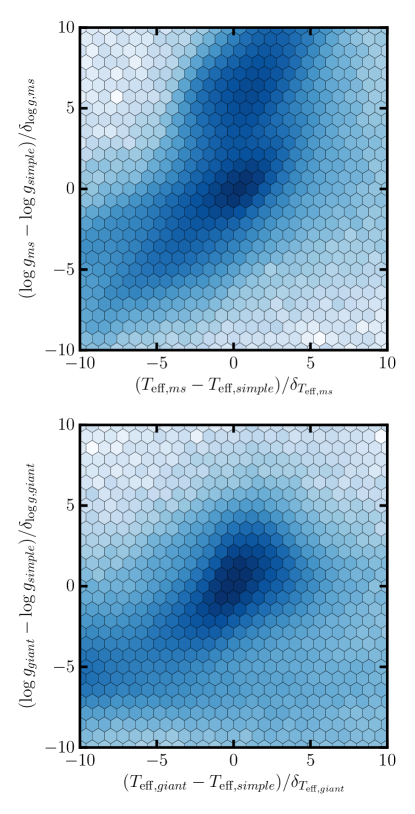
Figure 4: The normalized differences in effective temperature $T_{\mathrm{eff}}$ and surface gravity $\log g$ between the main-sequence model and the simple model (top panel), and the giant model and the simple model (bottom panel). The density scaling is logarithmic, and the differences in $T_{\mathrm{eff}}$ and $\log g$ are scaled to make them approximately isotropic (see text for details). The peak at $(0,0)$ represents good agreement between the simple model and comparison model, whereas the over-densities elsewhere are a consequence of testing the model on stars very different to the training set (e.g., dwarf stars tested on a model trained with only giant stars).

In Figure 4 we show the differences in effective temperature $T_{\mathrm{eff}}$ and surface gravity $\log g$ between: the main-sequence model (Section 3.4) and the simple model (Section 3.3); and the differences between the red giant branch model (Section 3.5) and the simple model (Section 3.3). We have scaled the differences in $T_{\mathrm{eff}}$ and $\log g$ to make the central peak near $(0,0)$ to be approximately isotropic by setting $\delta_{T_{\rm eff}}=90$ K for the main-sequence model, $\delta_{T_{\rm eff}}=50$ K for the giant model, and $\delta_{\log{g}}=0.15$ dex for both models. It is important to note that these $\delta$ values do not represent any kind of intrinsic uncertainty or precision: they are merely normalization factors. Adopting substantially different scaling factors would produce in clear inconsistencies in our results (e.g., sub-giants being misclassified as giants). Therefore we chose these factors empirically to make the distributions in Figure 4 approximately isotropic, and to some extent, comparable. In Figure 4 the stars within the peak at $(0,0)$ represent objects where the simple model and the comparison model both report similar labels. The artefacts seen in the Hertzsprung-Russell diagrams in Figure 2 are also present in Figure 4 as over-densities far away from the central peak. Therefore, we can adopt the scaled distance in labels $T_{\mathrm{eff}}$ and $\log g$ from the simple model to the main-sequence model $d_{ms}$,

$$d_{ms} = \left(\frac{T_{{\rm eff},ms}-T_{{\rm eff},simple}}{\delta_{T_{{\rm eff},ms}}}\right)^{2}+\left(\frac{\log{g}_{ms}-\log{g}_{simple}}{\delta_{\log{g},ms}}\right)^{2}\quad,$$ (7)

and the scaled distance from the simple model to the giant model $d_{giant}$,

$$d_{giant} = \left(\frac{T_{{\rm eff},giant}-T_{{\rm eff},simple}}{\delta_{T_{{\rm eff},giant}}}\right)^{2}+\left(\frac{\log{g}_{giant}-\log{g}_{simple}}{\delta_{\log{g},giant}}\right)^{2}\quad,$$ (8)

to derive the weights,

$$w_{ms}=\frac{1}{{d_{ms}}^{2}} w_{giant}=\frac{1}{{d_{giant}}^{2}}\quad,$$ and (9)

and produce the weighted labels $\hat{\ell}$:

$$\hat{\ell}=\frac{w_{ms}\,\ell_{ms}+w_{giant}\,\ell_{giant}}{w_{ms}+w_{giant}}\quad.$$ (10)

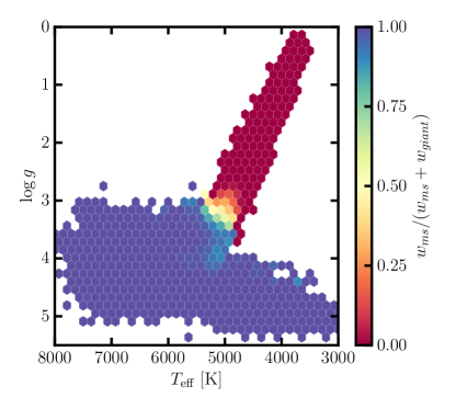
Figure 5: The mean relative main-sequence model weight $w_{ms}/(w_{ms}+w_{giant})$ at each hexagonal bin of weighted effective temperature $T_{\mathrm{eff}}$ and surface gravity $\log g$. The relative weighting illustrates how only results from the main-sequence model are adopted for unevolved stars, and there is a gradual transition to using results from the giant model, before only results from the giant model are used for evolved stars.

We calculate weighted errors of $\hat{\ell}$ in the same manner. In Figure 5 we show the mean relative weight $w_{ms}/(w_{ms}+w_{giant})$ within each two-dimensional hexagonal bin of $\hat{T}_{\mathrm{eff}}$ and $\hat{\log}g$. Hereafter when we refer to labels (e.g., $T_{\mathrm{eff}}$), we refer to those from the joint estimate $\hat{\ell}$, not individual estimates from separate models. For giant stars the relative weight of the main-sequence model is zero, and vice-versa for main-sequence stars. The relative weights smoothly transition from 0 to 1 on the sub-giant branch near $\log{g}\approx 3.5$, in the training set overlap region of both models. For abundance labels in the giant model that are not in the main-sequence model (e.g., [O/H], [Mg/H]), we only report abundances for objects if $w_{ms}<0.05$.

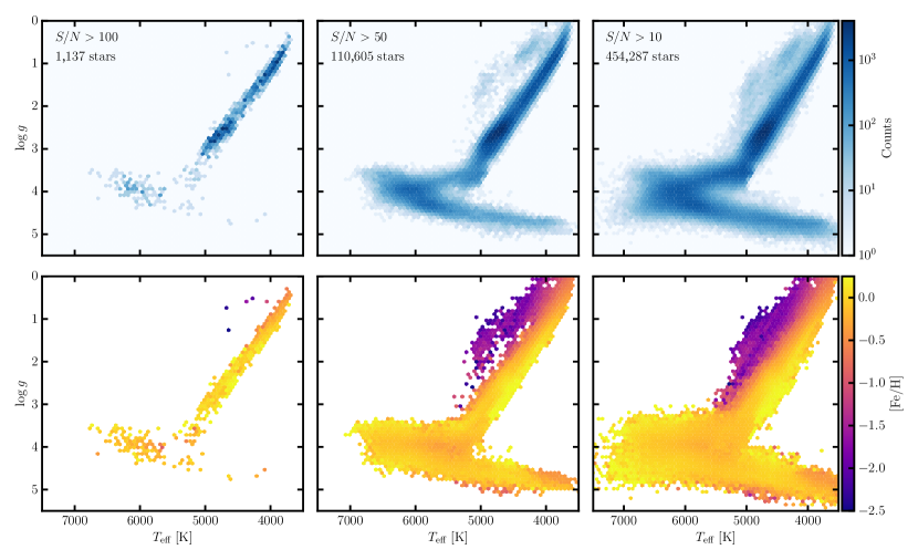
Figure 6: The effective temperature $T_{\mathrm{eff}}$ and surface gravity $\log g$ for RAVE stars after combining labels from the main-sequence and giant star models. Only results meeting our quality constraints are shown (see Section 5). The top three panels show logarithmic density, and bins in the bottom three panels are colored by the median metallicity in each bin.

The weighted $T_{\mathrm{eff}}$ and $\log g$ values for stars meeting different S/N constraints are shown in Figure 6, both in logarithmic density and mean metallicity. The artefacts from individual models are no longer apparent, and the complete structure of the Hertzsprung-Russell diagram is visible. However, there are a number of caveats introduced by the decisions we have made on how to combine estimates from multiple models. We discuss these issues in detail in Section 5.

4 Validation experiments

In addition to the cross-validation tests that we have previously described, we have conducted a number of internal and external validation experiments to test the validity of our results. We will begin by describing internal validation tests based on repeat observations, before evaluating our accuracy based on high-resolution literature comparisons.

4.1 Internal validation

4.1.1 Repeat observations

The RAVE survey performed repeat observations for 43,918 stars with time intervals ranging from a few hours to up to four years. This timing was constructed to be quasi-logarithmic such that spectroscopic binaries could be optimally identified. Most of the stars that were observed multiple times were only observed twice, with thirteen visits being the maximum number of observations for any target. These repeat observations allow us to quantify the level of (in)correctness in our formal errors.

We calculated all possible pair-wise differences between the labels we derived from multiple visits. If RAVE observed a star $H$ times, there are $H!/2(H-2)!$ possible $a$-to-$b$ pair-wise combinations where we can calculate the difference between the derived label (for example, $\log g$) over the quadrature sum of their formal errors $(\log g_{a}-\log g_{b})/\sqrt{{\sigma_{\log g,a}}^{2}+{\sigma_{\log g,b}}^{2}}$. If our derived labels were unbiased and our formal errors were correct, the distribution of these pair-wise comparisons would be well-represented by a Gaussian distribution with zero mean and variance of unity. However, our formal errors are likely to be under-estimated, and therefore we introduce a systematic error floor for each label, which is added in quadrature to every observation such that (for example, $\log g$),

$$\eta_{\log g} = \frac{\log g_{a}-\log g_{b}}{\sqrt{{\sigma_{\log g,a}}^{2}+{\sigma_{\log g,b}}^{2}+2{\sigma_{\log g,floor}}^{2}}}\quad.$$ (11)

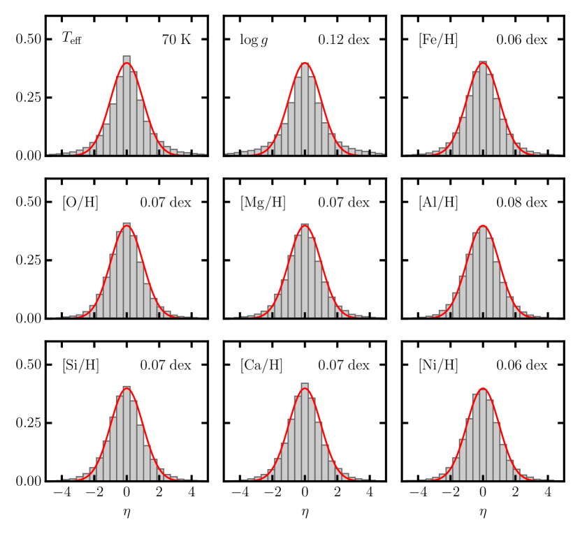
Figure 7: Distribution of differences in label estimates from multiple visits, divided by the quadrature sum of their formal errors, and a minimum error value for each observation. If our measurements were unbiased and our errors were representative, no minimum error floor would be required and the distribution of $\eta$ would by normally-distributed with zero mean and unity variance. We increased the error floor for each label until the variance in the distribution of $\eta$ approximately reached unity. Derived error floors are shown for each label.

We increased the minimum label error until the variance of the $\eta$ distribution approximately reached unity. We found the minimum error in $T_{\mathrm{eff}}$ to be 70 K, 0.12 dex in $\log g$, and varied between 0.06–0.08 dex for individual elements. The minimum errors are given with the distributions of $\eta$ for each label in Figure 7. These minimum values form part of our error model, such that they have been added in quadrature with the formal errors; the quoted label errors in our catalog include these minimum errors.

4.1.2 Precision as a function of S/N ratio

We further used the repeat observations in RAVE to build intuition for the label precision that was achievable as a function of S/N ratio. Specifically we stacked all spectra for a given star by summing the fluxes weighted by the inverse variances, then treated the stacked spectra as normal survey stars. We inferred labels for the stacked spectra using all three models, and derived a joint estimate as per Section 3.6. The labels we inferred from each stacked spectrum then served as a basis of comparison for the labels we derived from the individual visit spectra of the same star, which are of lower S/N ratios.

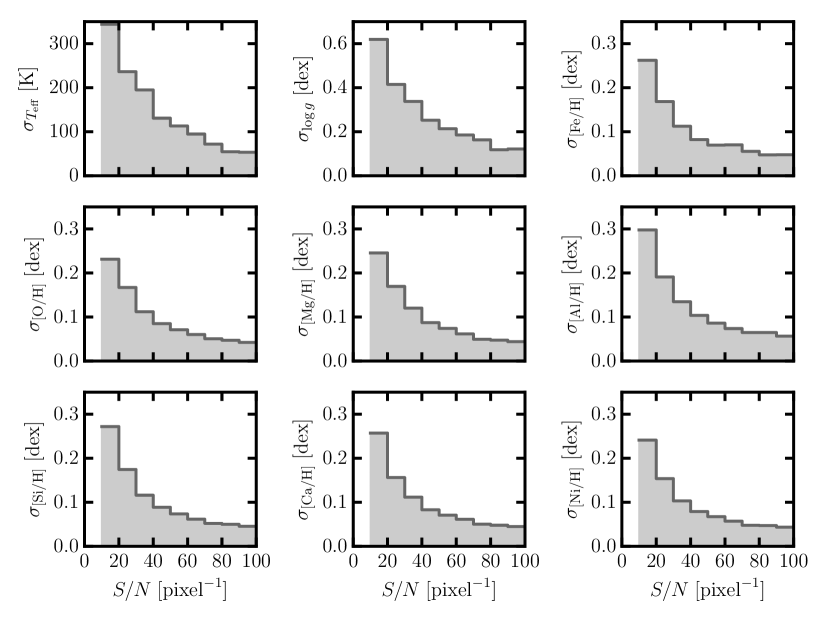
Figure 8: The RMS deviation of labels for repeated observations in the test set. The RMS deviation is binned as a function of the S/N ratio of the individual visit spectra. The precision flattens out at S/N $\gtrsim 40$ pixel^-1, where our results become systematics-limited.

In Figure 8 we show the RMS difference in labels between the stacked spectra and single visit, binned by the S/N ratio of the individual visit spectrum. Here we only show stars where the stacked spectrum had S/N $>100$ pixel^-1 to ensure that our baseline comparisons were in a region where we are dominated by systematic uncertainties. The precision in all labels tends to flatten out past S/N $>40$ pixel^-1, and the precision at high S/N ratios is comparable to the minimum error floors we adopted in Section 4.1.1. The median S/N of RAVE spectra is 50 pixel^-1, at which point our abundance precision is about 0.07 dex, varying a few tenths of a dex between different elements.

4.2 External validation

4.2.1 Comparison with RAVE DR4

We cross-matched our results against the official fourth RAVE data release as an initial point of external comparison (Figure 9). In order to provide a fair comparison, we only show stars that meet a number of quality flags in both samples. Our constraints require that the S/N ratio exceeds 10 pixel^-1, and $\chi_{r}^{2}<3$. For this comparison we further required that: the QK flag from Kordopatis et al. (2013) is zero, indicating no problems were reported by the pipeline; $T_{{\rm eff},DR4}>4000$ K; the error in radial velocity e_HRV is $<$8 km s^-1; and the three principal morphological flags c1, c2, c3, from Matijevič et al. (2012) all indicate ‘n’ for a normal FGK-type star. There is good agreement in $T_{\mathrm{eff}}$, with a bias and RMS of just 4 K and 240 K, respectively. The offset in $\log g$ on the giant branch between this study and Kordopatis et al. (2013) has been noted in other studies (e.g., APOGEE), and this issue has been minimized in the fifth RAVE data release by correcting $\log g$ values with a calibration sample consisting of asteroseismic targets and the Gaia benchmark stars. There is also a slight discrepancy in the $\log g$ values along the main-sequence, where our work tends to taper down towards higher $\log g$ values at cooler temperatures, and the RAVE DR4 sample tends to have a slightly flatter lower main-sequence. This difference is not likely to have a very significant effect on the detailed abundance or spectrophotometric distance determinations between these studies (Binney et al., 2014).

4.2.2 Comparisons with Reddy, Bensby, and Valenti & Fischer

We searched the literature for studies that overlap with RAVE, and which base their analysis on high-resolution, high S/N spectra. We found four notable studies with a sufficient level of overlap: the Milky Way disk studies by Reddy et al. (2003, 2006) and Bensby et al. (2014), as well as the Valenti & Fischer (2005) work on exoplanet host star candidates. These studies perform a careful (manual; expert) analysis using extremely high-resolution, high S/N spectra, and make use of Hipparcos parallaxes where possible. Most of the stars in these samples are main-sequence or sub-giant stars. Therefore, these works constitute an excellent comparison to evaluate the accuracy of our results on the main-sequence and sub-giant branch.

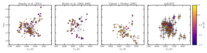
Figure 10: Hertsprung-Russell diagrams of stars in common between this work and that of Bensby et al. (2014); Reddy et al. (2003, 2006); Valenti & Fischer (2005). Stars are colored by the metallicity of each study. Circles indicate literature markers in the first three panels, and the linked triangles indicate RAVE-on parameters for the same object. This figure illustrates the good qualitative agreement in the shape of the turnoff and sub-giant branch.

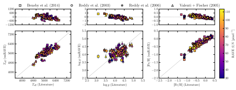
Figure 11: Stellar parameter ($T_{\mathrm{eff}}$, $\log g$, [Fe/H]) comparisons for stars in common between this work and ‘gold standard’ studies that use high-resolution, high S/N spectra and Hipparcos parallaxes where available: Bensby et al. (2014); Reddy et al. (2003, 2006); Valenti & Fischer (2005). Stars are colored by the S/N of the RAVE spectra.

In Figure 10 we show Hertzsprung-Russell diagrams for the RAVE stars that overlap with these studies. We only include stars with $\chi_{r}^{2}<3$ and $S/N>10$ pixel^-1, although the latter cut removed only a few stars because the average S/N in the RAVE spectra for these stars is relatively high ($\gtrsim{}50$ pixel^-1). The literature data points in Figure 10 are linked to our derived labels for the same stars, illustrating good qualitative agreement across the turn-off and sub-giant branch in all studies. If we treat all three studies as a single point of comparison, the bias between our work and these studies is $-89$ K in $T_{\mathrm{eff}}$, just $-0.06$ dex in $\log g$, and $-0.03$ dex in [Fe/H] (see Figure 11). The RMS deviation in labels is 237 K, 0.30 dex, and 0.15 dex, respectively. When considering the relative information content available in RAVE (945 pixels in the near infrared with $\mathcal{R}\approx 7{,}500$) compared to these literature studies that use Hipparcos parallaxes where possible, and base their inferences on spectra with resolving power $\mathcal{R}$ between 40,000 to 110,000, and S/N ratios exceeding 150, we consider the agreement to be very satisfactory. Indeed, given the metallicity precision available in the RAVE-on catalog, these results will likely be useful for future studies based on exoplanet host star properties (e.g., TESS).

4.2.3 Comparison with the Gaia-ESO survey

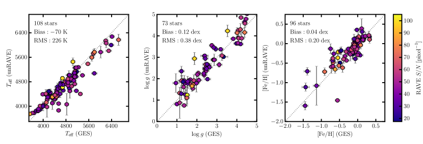
Figure 12: Stellar parameter ($T_{\mathrm{eff}}$, $\log g$, [Fe/H]) comparison between the fourth internal data release from the Gaia-ESO survey, and this work. The number of stars in each panel are shown, as well as the bias and RMS deviation in each label. Stars are colored by the S/N of the RAVE spectra. Most of the Gaia-ESO/RAVE overlap stars have relatively low S/N ratios in RAVE, near $\approx 30$ pixel^-1.

There are 142 stars that overlap between RAVE and the fourth internal data release of the Gaia-ESO survey. These are a mix of main-sequence, sub-giant and red giant branch stars. About half (67) of the sample were acquired with the UVES instrument — the other with the GIRAFFE spectrograph — and the S/N of the Gaia-ESO spectra peaks at $\approx 140$ pixel^-1. Despite most of these stars having relatively low S/N ratios in RAVE ($\approx 25$ pixel^-1), there is good agreement in with Gaia-ESO and the RAVE-on stellar parameters (Figure 12). The RMS in effective temperature, surface gravity and metallicity is 233 K, 0.37 dex, and 0.17 dex, respectively.

Based on this comparison, we find no evidence for a systematic offset in metallicities between stars on the main-sequence and those on the giant branch. This is a crucial observation, as the metallicities for stars in our main-sequence training set have a principally different source to those on the giant branch. We cannot make these same inferences based on other surveys, like APOGEE, because (1) APOGEE stars formed part of the training set, and (2) they do not include main-sequence stars. Even if we found good agreement between K2/EPIC and APOGEE metallicities, this would not be informative, because APOGEE is the source of metallicity for many stars on the giant branch in the K2/EPIC sample. Therefore, although this is a qualitative comparison only, it is reassuring that there is no obvious systematic difference between the metallicities of main-sequence and giant branch stars.

The metallicity agreement between this work and Gaia-ESO extends down to low metallicity, near $[{\rm Fe/H}]\approx-1.5$. The scatter increases for the few stars in the overlap sample with $[{\rm Fe/H}]<-1$, in the regime where the influence from atomic transitions of these elements becomes very small in RAVE spectra. Moreover, these particular stars have lower S/N ratios, which is reflected in the larger uncertainties reported for these metallicities.

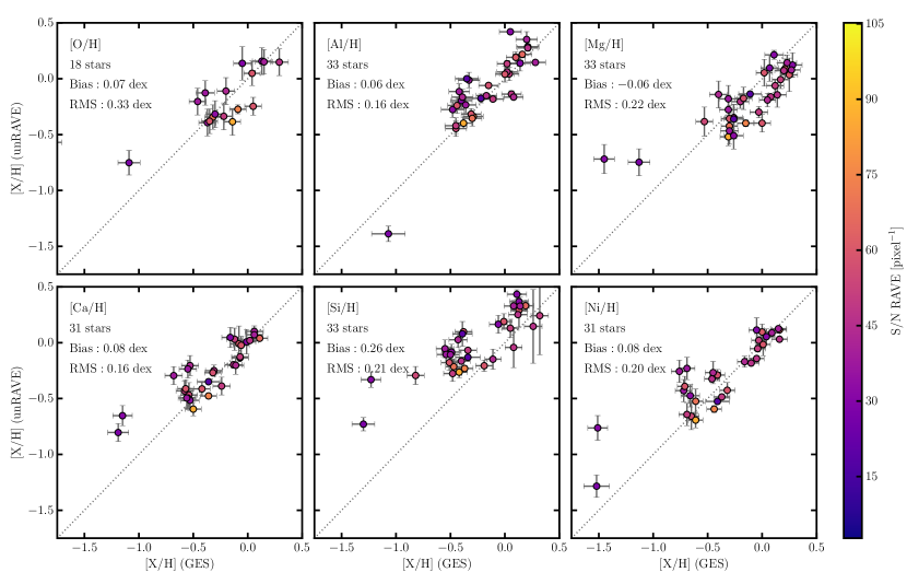
Figure 13: Detailed chemical abundances in the fourth internal data release from the Gaia-ESO survey compared to this work. The number of stars shown in each panel is indicated, and the bias and RMS deviations are shown. Stars are colored by the S/N of the RAVE spectra.

The fourth internal data release of the Gaia-ESO includes detailed chemical abundances of up to 45 species ($\approx 32$ elements at different ionization stages). This provides us with an independent validation for our detailed abundances on the giant branch. These comparisons are shown in Figure 13, where markers are colored by the S/N of the RAVE spectrum. The number of stars available in each abundance comparison varies due to what is available in the Gaia-ESO data release, which is itself a function of the instrument used, the spectral type, and other factors. The absolute bias for individual elements varies from as low as 0.06 dex ([Al,Mg/H]) to as high as 0.26 dex ([Si/H]), where we over-estimate [Si/H] abundances relative to the Gaia-ESO survey. The large bias in [Si/H] is likely a consequence of an offset between [Si/H] abundances in Gaia-ESO and APOGEE, the source of our training set for giant star abundances. The RMS deviation in each label is small for stars with [X/H] $>-0.5$, before increasing at lower metallicities. If we consider all stars, the smallest abundance RMS we see with respect to Gaia-ESO is 0.16 dex for [Ca/H] and [Al/H]. The increasing RMS at low metallicity is likely a consequence of multiple factors, namely: inaccurate abundance labels for metal-poor stars (Section 3.2); only weak, blended lines being available in RAVE, which cease to be visible in hot and/or metal-poor stars; and to a lesser extent, low S/N ratios for those particular stars being compared. Unfortunately not all of these factors are represented by the quoted errors in each label. For these reasons, although it affects only a small number of stars, we recommend caution when using individual abundances for very metal-poor giant stars in our sample.

4.2.4 Comparison with the RAVE DR4 calibration sample

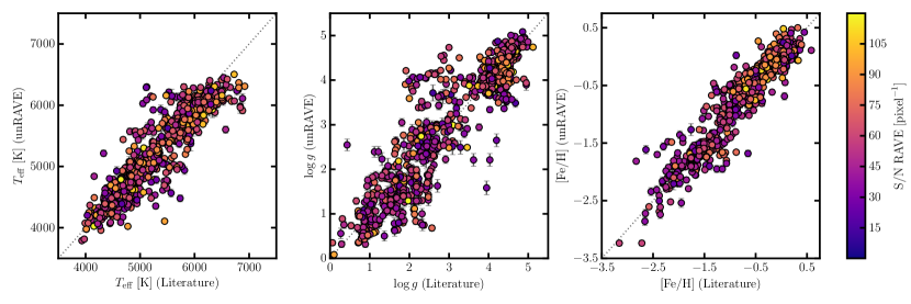
Figure 14: Stellar parameter ($T_{\mathrm{eff}}$, $\log g$, [Fe/H]) comparison with the literature calibration sources used by Kordopatis et al. (2013) and Kunder et al. (2016). Stars are colored by the S/N of the RAVE spectra. Note that this comparison is for illustrative purposes only: it is not an indication of independent agreement with the literature because some metal-poor stars in this literature sample were used in the construction of our training set (see text for details).

The fourth RAVE data release made use of a number of high-resolution studies to verify the accuracy of their derived stellar atmospheric parameters. These samples include main-sequence stars, giant stars, with a particular focus to include metal-poor stars to identify (and correct) any deviations at low metallicities. We refer the reader to Kordopatis et al. (2013) for the full compilation of literature sources. Although the stellar atmospheric parameters in this compilation come from multiple (heterogeneous) sources, we find generally good agreement with these works (Figure 14). However, we note that some reservation is warranted when evaluating this comparison, as some of the metal-poor stars in this calibration sample formed part of our training set.

4.3 Astrophysical validation

4.3.1 Globular clusters

After verifying that our atmospheric parameters and abundances are comparable with high-resolution studies, here we verify that our results are consistent with expectations from astrophysics. In the RAVE survey, Anguiano et al. (2015) identified 70 stars with positions and radial velocities that are consistent with being members of globular clusters: 49 stars belonging to NGC 5139 ($\omega$ Centauri), 11 members of the retrograde globular cluster NGC 3201, and 10 members of NGC 362. In addition, Kunder et al. (2014) compiled 12 stars thought to belong to NGC 1851, and a further 10 stars in NGC 6752. We refer the reader to those studies for details regarding the membership selection.

In Figure 15 we show our effective temperature $T_{\mathrm{eff}}$ and surface gravity $\log g$ for these prescribed globular cluster members. The right-hand panels indicate measurements made in this work, and for comparison purposes we have included the results from the fourth RAVE data release in the left-hand panels. We show representative PARSEC isochrones (Bressan et al., 2012) in all panels, where the isochrone ages and metallicities are adopted from Kunder et al. (2016); Marín-Franch et al. (2009), and the Harris (1996, accessed 6 September 2016) catalog of globular cluster properties. The globular cluster with the most number of members is NGC 5139 ($\omega$-Centauri), where we find a significant metallicity spread that is consistent with high-resolution studies (Marino et al., 2011; Carretta et al., 2009, 2013). Based on the pre-defined membership criteria, we find the mean metallicity of $\omega$-Centauri to be $[{\rm Fe/H}]=-0.85$. However, it is clear that the membership criteria could be improved with our revised metallicities and detailed chemical abundances. Indeed, our individual abundance labels could be further used to identify globular cluster members — at least, of relatively metal-rich clusters — that are now tidally disrupted (Anguiano et al., 2016; Kuzma et al., 2016; Navin et al., 2016), even for stars with low S/N ratios.

4.3.2 Open clusters

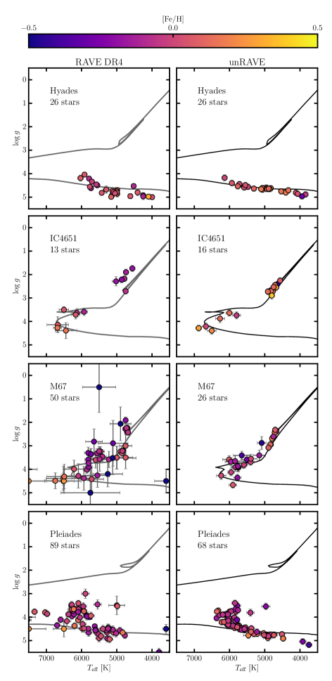
Figure 16: Effective temperature $T_{\mathrm{eff}}$ and surface gravity $\log g$ for open cluster members identified by (Kunder et al., 2016). Left-hand panels indicate results from the fourth RAVE data release (Kordopatis et al., 2013), and the right-hand panels show results from this work. A representative isochrone is shown for each cluster (Bressan et al., 2012).

Using positions, proper motions, and metallicities from the RAVE survey (i.e., not ours, such that they can be used as comparison), we identify $\sim$160 probable members of four open clusters that were observed by RAVE. Specifically we identify 78 potential Pleiades members, 26 candidates in the Hyades, another 13 in IC4561, and 30 stars in the solar-metallicity open cluster M67. We show the effective temperature $T_{\mathrm{eff}}$ and surface gravity $\log g$ for these cluster candidates in Figure 16. The isochrones are sourced from Bressan et al. (2012), with cluster properties adopted from Kharchenko et al. (2013).

We find good agreement between our atmospheric parameters (right-hand panels) and the isochrones shown. The position of the red clump in IC4651 and M67 are perfectly matched to the isochrone, and the Hyades main-sequence is in good agreement down to $T_{\rm eff}\approx 4000$ K. Similarly, we find consistency with the literature and our metallicity scale. We find the mean metallicity of M67 stars to be $[{\rm Fe/H}]=-0.02\pm 0.03$ dex, in excellent agreement with the expected $[{\rm Fe/H}]=0.00$ value (not accounting for atomic diffusion). We further find the Hyades mean metallicity to be $[{\rm Fe/H}]=0.07\pm 0.09$ dex, consistent with Paulson et al. (2003): $[{\rm Fe/H}]\approx 0.13$. For IC4651 from 13 stars we find a mean $[{\rm Fe/H}]=0.15\pm 0.03$ dex, matching the high-resolution, high S/N study of Pasquini et al. (2004), where they find $[{\rm Fe/H}]=0.10\pm 0.03$ dex. Finally, from 78 stars we find the mean metallicity of the Pleiades to be $[{\rm Fe/H}]=-0.02\pm 0.01$ dex, in very good agreement with the $[{\rm Fe/H}]=-0.034\pm 0.024$ dex measurement reported by Friel & Boesgaard (1990).

Despite the discrepancies between the isochrone and our derived labels for stars in the Pleiades, we have made no attempt to refine the membership selection in any of the aforementioned clusters. We note however, that the same discrepancy with the isochrone appears present in the fourth RAVE data release Kordopatis et al. (2013).

5 Discussion

We have performed an independent re-analysis of 520,781 RAVE spectra, having derived atmospheric parameters ($T_{\mathrm{eff}}$, $\log g$, [Fe/H]) for all stars, as well as detailed chemical abundances for red giant branch stars. When combined with the TGAS sample, these results amount to a powerful compendium for chemo-dynamic studies of the Milky Way. However, our analysis has caveats. Inferences based on these results should recognize those caveats, and acknowledge that these results are subject to our explicit assumptions, some of which are provably incorrect.

For practical purposes we adopted separate models: one for the giant branch and one for the main-sequence. A third model was used to derive relative weights for which results to use. The relative weighting we have used does not have any formal interpretation as a likelihood or belief (in any sense): it was introduced for practical reasons to identify systematic errors and combine results for multiple models. Because the relative weights have no formal interpretation, it is reasonable to consider this method is as ad hoc as any other approach. The relative weighting has no warranty to be (formally) correct, and therefore may introduce inconsistencies or systematic errors rather than minimizing them.

If we only consider the results from individual models, there are a number of cautionary remarks that stem from the construction of the training set. The labels for red giant branch stars primarily come from APOGEE, where previous successes with The Cannon have demonstrated that APOGEE labels based on high S/N data can be of high fidelity (Ness et al., 2015, 2016; Ho et al., 2016; Casey et al., 2016). However, the lack of metal-poor stars in the APOGEE/RAVE overlap sample produced a tapering-off in the test set — where no stars had reliably reported metallicities below that of the training set — which forced us to construct a heterogeneous training set. The metal-poor stars included in this sample are from high-resolution studies (Fulbright et al., 2010; Ruchti et al., 2011), but it is not known if the stellar parameters are of high fidelity because we have a limited number of quality statistics available. Moreover, there is no guarantee that the stellar parameters or abundances are on the same scale as APOGEE (and good reasons to believe they will not be; see Smiljanic et al., 2014).

If the metallicities of metal-poor giant stars were on the same scale as the APOGEE abundances, there is a larger issue in verifying that the main-sequence metallicities and giant branch metallicities are on the same scale. The training set for the main-sequence stars includes metallicities from a variety of sources, including LAMOST, and the fourth RAVE data release. Even on expectation value, there is no straightforward manner to ensure that the main-sequence model and the red giant branch model produce metallicities on the same scale. We see no systematic offset in metallicities of dwarf and giant stars that overlap between RAVE and the Gaia-ESO survey, suggesting that if there is a systematic offset, it must be small. Nevertheless, these are only verification checks based on $<1$% of the data, and there is currently insufficient data for us to prove both models are on the same abundance scale.

For some of the most metal-poor giant stars in RAVE  we know the abundances are not on the same scale as APOGEE, because we were forced to adopt abundances for specific elements when they were unavailable. Although we sought to adopt mean level of Galactic chemical enrichment at a given overall metallicity, this is not a representative abundance. Even if that is the mean enrichment at that Galactic metallicity, there is no requirement for zero abundance spread. More fundamentally, we are incorrectly asserting that the element must be detectable in the photosphere of the star. There may be no transition that is detectable in that star, even with zero noise, because it is too weak to have any effect on the spectrum. In the most optimistic case, this could be considered to be forcing the model to make use of correlated information between abundances. In a more representative (pessimistic) case, we are simply invoking what all abundances should be at low metallicity.

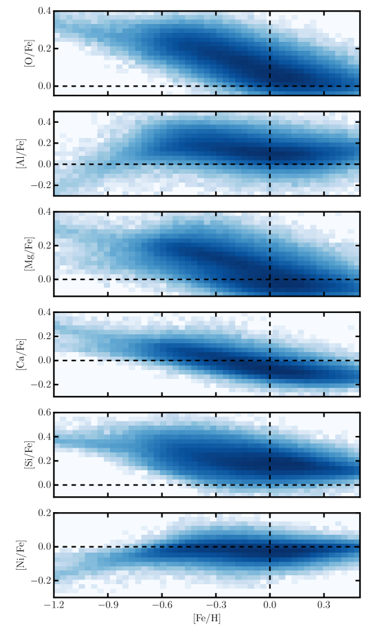
Figure 17: Detailed chemical abundances ([X/Fe]) for giant stars in RAVE-on with respect to [Fe/H], showing the Galactic chemical evolution derived for each element. Bin densities are scaled logarithmically. Note that the y-axis limits vary for each panel, however for clarity we show the scaled-solar position by dashed lines, and have common tick mark spacing on the y-axis for all panels. Only stars meeting our quality constraints are shown (see Section 5).

This choice is reflected in the abundances of the test set. While we do recover trustworthy metallicities for ultra metal-poor ($[{\rm Fe/H}]\lesssim-4$) stars like CD-38 245, the individual abundances for all extremely metal-poor stars aggregate (in [X/Fe] space; Figure 17) at the assumed abundances for the metal-poor stars in our sample. Thus, while the overall metallicities appear reliable, the individual abundances for extremely metal-poor stars in the test set cannot be considered trustworthy in any sense. For this reason we have updated the electronic catalog to discard these results as erroneous.

In Section 3 we assumed that any fibre- or time-dependent variations in the RAVE spectra are negligible. This is provably incorrect. Indeed, Kordopatis et al. (2013) note that the effective resolution of RAVE spectra varies from $6{,}500<\mathcal{R}<8{,}500$, and that the effective resolution is a function of temperature variations, fibre-to-fibre variations, and thus position on the CCD (Steinmetz et al., 2006). For this reason we ought to expect our derived stellar parameters or abundances to be correlated either with the fibre number, with the observation date, or both. If significant, the trend could produce systematically offset stellar abundances solely due to the fibre used. Kordopatis et al. (2013) conclude that resolution-based effects on the RAVE stellar parameters should be a second-order effect. We have not seen evidence of these resolution-based correlations in our results, however, we have only performed cursory (non-exhaustive) experiments to investigate this issue.

We have shown some potential outcomes when the test set spectra differ significantly from the spectra in the training set. Test set spectra that is ‘unusual’ from the training set can be projected as peculiar artefacts in label space. In other words, unusual spectra can appear as ‘clumps’ in regions of parameter space that we could consider as being normal (e.g., an over-density of solar-type stars). We addressed this issue for the main-sequence and giant models by using a third model (Section 3.3) to calculate relative weights. However, spectra that are unusual from the training set used in the simple model could still project as systematic artefacts in label space.

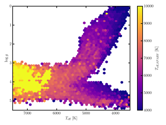
Figure 18: Effective temperatures $T_{\mathrm{eff}}$ and surface gravities $\log g$ from this work, where each hexagonal bin is colored by the maximum temperature for any star in that bin, as reported by the RAVE pre-processing pipeline SPARV (Steinmetz et al., 2006; Zwitter et al., 2008). Hot stars are not included in our training set, and appear above the turnoff in our labels. For this reason, we supply a boolean quality control flag QC that flags stars (as False, for failing to meet our quality constraints) with $T_{\mathrm{eff}}>8000$ K (as reported by SPARV), or results that do not meet other minimum constraints (see Section 5 for details).

Indeed, there are two known artefacts in our data that are relevant to this discussion. The first is a small over-density at the base of the giant branch, which is likely a consequence of joining the 9-label and 3-label models. The second has an astrophysical origin: there are no hot stars ($T_{\mathrm{eff}}>8000$ K) present in our training set, yet there are many in the RAVE survey. However, the RAVE pre-processing pipeline (SPARV; Steinmetz et al., 2006; Zwitter et al., 2008) performs template matching against grids of cool and hot stars, and therefore we can use that information to identify hot stars. In Figure 18 we show our derived effective temperatures $T_{\mathrm{eff}}$ and surface gravities $\log g$, where each hexagonal bin is colored by the maximum temperature reported by SPARV for any star in that bin. We show the maximum temperature reported by SPARV to demonstrate that hot stars project into a single clump in our label space — near the turn-off — in a region where we may otherwise be deceived into thinking the observed over-density is consistent with expectations from astrophysics.

This line of reasoning extends to spectra with other peculiar characteristics (e.g., chromospheric emission), and for these reasons we recommend the use of additional metadata to investigate possible artefacts. In our catalog we have included a column containing a boolean flag to indicate whether the labels pass very weak quality constraints. Specifically, we flag results as failing our quality constraints if SPARV indicates a $T_{\mathrm{eff}}>8000$ K, or if $\chi_{r}^{2}>3$, or if $S/N<10$ pixel^-1. These quality constraints represent the minimum acceptable conditions and should not be taken verbatim: judicious use of the morphological classifications (Matijevič et al., 2012) or additional metadata from the RAVE pre-processing pipelines is strongly encouraged.

We have presented a comprehensive collection of precise stellar abundances for stars in the first Gaia data release. In total we derive stellar atmospheric parameters for 441,397 stars, and report more than 1.69 million abundances. Despite the caveats and limitations discussed here, our validation experiments and comparisons with high-resolution spectroscopic studies suggests that our results have sufficient accuracy and precision to be useful for chemo-dynamic studies that become imminently feasible only in the era of Gaia data. We are optimistic that the RAVE-on catalog will advance understanding of the Milky Way’s formation and evolution.

Access the results electronically

Source code for this project is available at https://www.github.com/AnnieJumpCannon/rave, and this document was compiled from revision hash 794a221 in that repository. Derived labels, associated errors, and relevant metadata are available electronically through the RAVE database from 19 September 2016 onwards. Please note that it is a condition of using these results that the RAVE data release by Kunder et al. (2016) must also be cited, as the work presented here would not have been possible without the tireless efforts of the entire RAVE collaboration, past and present.

Figure 9: Stellar parameter ($T_{\mathrm{eff}}$, $\log g$, [Fe/H]) comparison between the fourth RAVE data release (Kordopatis et al., 2013) and this work. Here we show the ‘calibrated’ metallicity (column c_M_H_K) from the RAVE survey. Only stars meeting quality constraints in both studies are shown (see text for details).

Figure 15: Effective temperature $T_{\mathrm{eff}}$ and surface gravity $\log g$ for globular cluster members identified by Kunder et al. (2014); Anguiano et al. (2015). Left-hand panels indicate results from the fourth RAVE data release (Kordopatis et al., 2013), and the right-hand panels show results from this work. A representative isochrone is shown for each cluster (Bressan et al., 2012).

¹Institute of Astronomy, University of Cambridge, Madingley Road, Cambridge CB3 0HA, UK
²Simons Center for Data Analysis, 160 Fifth Avenue, 7th floor, New York, NY 10010, USA
³Center for Cosmology and Particle Physics, Department of Physics, New York University, 4 Washington Pl., room 424, New York, NY 10003, USA
⁴Center for Data Science, New York University, 726 Broadway, 7th floor, New York, NY 10003, USA
⁵Max-Planck-Institut für Astronomie, Königstuhl 17, D-69117 Heidelberg, Germany
⁶University of Ljubljana, Faculty of Mathematics and Physics, Jadranska 19, 1000 Ljubljana, Slovenia
⁷Research School of Astronomy and Astrophysics, Mount Stromlo Observatory, The Australian National University, ACT 2611, Australia
⁸Mullard Space Science Laboratory, University College London, Holmbury St Mary, Dorking, RH5 6NT, UK
⁹Observatoire astronomique de Strasbourg, Université de Strasbourg, CNRS, UMR 7550, 11 rue de l’Université, F-67000 Strasbourg, France
¹⁰Sydney Institute for Astronomy, School of Physics, University of Sydney, NSW 2006, Australia
¹¹E.A. Milne Centre for Astrophysics, University of Hull, Hull, HU6 7RX, United Kingdom
¹²Astronomisches Rechen-Institut, Zentrum für Astronomie der Universität Heidelberg, Mönchhofstr. 12–14, 69120 Heidelberg, Germany
¹³Kapteyn Astronomical Institute, University of Groningen, P.O. Box 800, 9700 AV Groningen, The Netherlands
¹⁴INAF Astronomical Observatory of Padova, 36012 Asiago (VI), Italy
¹⁵Department of Physics and Astronomy, University of Victoria, Victoria, BC, Canada V8P 5C2
¹⁶Senior CIfAR Fellow
¹⁷Department of Physics and Astronomy, Macquarie University, Sydney, NSW 2109, Australia
¹⁸Western Sydney University, Penrith South DC, NSW 1797
¹⁹Johns Hopkins University, Baltimore, MD, USA

References

- Anguiano et al. (2015) Anguiano, B., Zucker, D. B., Scholz, R.-D., et al. 2015, MNRAS, 451, 1229
- Anguiano et al. (2016) Anguiano, B., De Silva, G. M., Freeman, K., et al. 2016, MNRAS, 457, 2078
- Astropy Collaboration et al. (2013) Astropy Collaboration, Robitaille, T. P., Tollerud, E. J., et al. 2013, Astronomy & Astrophysics, 558, AA33
- Bensby et al. (2014) Bensby, T., Feltzing, S., & Oey, M. S. 2014, A&A, 562, A71
- Binney et al. (2014) Binney, J., Burnett, B., Kordopatis, G., et al. 2014, MNRAS, 437, 351
- Boeche et al. (2011) Boeche, C., Siebert, A., Williams, M., et al. 2011, AJ, 142, 193
- Boeche et al. (2013) Boeche, C., Chiappini, C., Minchev, I., et al. 2013, A&A, 553, A19
- Bressan et al. (2012) Bressan, A., Marigo, P., Girardi, L., et al. 2012, MNRAS, 427, 127
- Bovy et al. (2016) Bovy, J., Rix, H.-W., Schlafly, E. F., et al. 2016, ApJ, 823, 30
- Brown et al. (2011) Brown, T. M., Latham, D. W., Everett, M. E., & Esquerdo, G. A. 2011, AJ, 142, 112
- Bouy et al. (2015) Bouy, H., Bertin, E., Sarro, L. M., et al. 2015, A&A, 577, A148
- Carretta et al. (2009) Carretta, E., Bragaglia, A., Gratton, R. G., et al. 2009, A&A, 505, 117
- Carretta et al. (2013) Carretta, E., Bragaglia, A., Gratton, R. G., et al. 2013, A&A, 557, A138
- Casagrande et al. (2011) Casagrande, L., Schönrich, R., Asplund, M., et al. 2011, A&A, 530, A138
- Casey et al. (2012) Casey, A. R., Keller, S. C., & Da Costa, G. 2012, AJ, 143, 88
- Casey et al. (2013) Casey, A. R., Da Costa, G., Keller, S. C., & Maunder, E. 2013, ApJ, 764, 39
- Casey et al. (2014a) Casey, A. R., Keller, S. C., Da Costa, G., Frebel, A., & Maunder, E. 2014, ApJ, 784, 19
- Casey et al. (2014b) Casey, A. R., Keller, S. C., Alves-Brito, A., et al. 2014, MNRAS, 443, 828
- Casey & Schlaufman (2015) Casey, A. R., & Schlaufman, K. C. 2015, ApJ, 809, 110
- Casey (2016) Casey, A. R. 2016, ApJS, 223, 8
- Casey et al. (2016) Casey, A. R., Hogg, D. W., Ness, M., et al. 2016, arXiv:1603.03040
- Cui et al. (2012) Cui, X.-Q., Zhao, Y.-H., Chu, Y.-Q., et al. 2012, Research in Astronomy and Astrophysics, 12, 1197
- De Silva et al. (2015) De Silva, G. M., Freeman, K. C., Bland-Hawthorn, J., et al. 2015, MNRAS, 449, 2604
- Deason et al. (2011) Deason, A. J., Belokurov, V., & Evans, N. W. 2011, MNRAS, 416, 2903
- Friel & Boesgaard (1990) Friel, E. D., & Boesgaard, A. M. 1990, ApJ, 351, 480
- Fulbright et al. (2010) Fulbright, J. P., Wyse, R. F. G., Ruchti, G. R., et al. 2010, ApJ, 724, L104
- García Pérez et al. (2016) García Pérez, A. E., Allende Prieto, C., Holtzman, J. A., et al. 2016, AJ, 151, 144
- Gilmore et al. (2012) Gilmore, G., Randich, S., Asplund, M., et al. 2012, The Messenger, 147, 25
- Harris (1996) Harris, W. E. 1996, AJ, 112, 1487
- Hawkins et al. (2016) Hawkins, K., Masseron, T., Jofre, P., et al. 2016, arXiv:1604.08800
- Holtzman et al. (2015) Holtzman, J. A., Shetrone, M., Johnson, J. A., et al. 2015, AJ, 150, 148
- Ho et al. (2016) Ho, A. Y. Q., Ness, M. K., Hogg, D. W., et al. 2016, arXiv:1602.00303
- Høg et al. (2000) Høg, E., Fabricius, C., Makarov, V. V., et al. 2000, A&A, 355, L27
- Huber et al. (2016) Huber, D., Bryson, S. T., Haas, M. R., et al. 2016, ApJS, 224, 2
- Jofré et al. (2015) Jofré, P., Mädler, T., Gilmore, G., et al. 2015, MNRAS, 453, 1428
- Kharchenko et al. (2013) Kharchenko, N. V., Piskunov, A. E., Schilbach, E., Röser, S., & Scholz, R.-D. 2013, A&A, 558, A53
- Kordopatis et al. (2011) Kordopatis, G., Recio-Blanco, A., de Laverny, P., et al. 2011, A&A, 535, A106
- Kordopatis et al. (2013) Kordopatis, G., Gilmore, G., Steinmetz, M., et al. 2013, AJ, 146, 134
- Kordopatis et al. (2015) Kordopatis, G., Binney, J., Gilmore, G., et al. 2015, MNRAS, 447, 3526
- Kunder et al. (2016) Kunder, A., et al. 2016, submitted
- Kunder et al. (2014) Kunder, A., Bono, G., Piffl, T., et al. 2014, A&A, 572, A30
- Kuzma et al. (2016) Kuzma, P. B., Da Costa, G. S., Mackey, A. D., & Roderick, T. A. 2016, MNRAS, 461, 3639
- Mädler et al. (2016) Mädler, T., Jofré, P., Gilmore, G., et al. 2016, arXiv:1606.03015
- Matijevič et al. (2012) Matijevič, G., Zwitter, T., Bienaymé, O., et al. 2012, ApJS, 200, 14
- Marino et al. (2011) Marino, A. F., Milone, A. P., Piotto, G., et al. 2011, ApJ, 731, 64
- Marín-Franch et al. (2009) Marín-Franch, A., Aparicio, A., Piotto, G., et al. 2009, ApJ, 694, 1498
- Michalik et al. (2015a) Michalik, D., Lindegren, L., & Hobbs, D. 2015, A&A, 574, A115
- Michalik et al. (2015b) Michalik, D., Lindegren, L., Hobbs, D., & Butkevich, A. G. 2015, A&A, 583, A68
- Munari et al. (2005) Munari, U., Sordo, R., Castelli, F., & Zwitter, T. 2005, A&A, 442, 1127
- Navin et al. (2016) Navin, C. A., Martell, S. L., & Zucker, D. B. 2016, arXiv:1606.06430
- Ness et al. (2012) Ness, M., Freeman, K., Athanassoula, E., et al. 2012, ApJ, 756, 22
- Ness et al. (2013a) Ness, M., Freeman, K., Athanassoula, E., et al. 2013, MNRAS, 430, 836
- Ness et al. (2013b) Ness, M., Freeman, K., Athanassoula, E., et al. 2013, MNRAS, 432, 2092
- Ness et al. (2015) Ness, M., Hogg, D. W., Rix, H.-W., Ho, A. Y. Q., & Zasowski, G. 2015, ApJ, 808, 16
- Ness et al. (2016) Ness, M., Hogg, D. W., Rix, H.-W., et al. 2016, ApJ, 823, 114
- Nordström et al. (2004) Nordström, B., Mayor, M., Andersen, J., et al. 2004, A&A, 418, 989
- Pasquini et al. (2004) Pasquini, L., Randich, S., Zoccali, M., et al. 2004, A&A, 424, 951
- Paulson et al. (2003) Paulson, D. B., Sneden, C., & Cochran, W. D. 2003, AJ, 125, 3185
- Randich et al. (2013) Randich, S., Gilmore, G., & Gaia-ESO Consortium 2013, The Messenger, 154, 47
- Recio-Blanco et al. (2016) Recio-Blanco, A., de Laverny, P., Allende Prieto, C., et al. 2016, A&A, 585, A93
- Reddy et al. (2003) Reddy, B. E., Tomkin, J., Lambert, D. L., & Allende Prieto, C. 2003, MNRAS, 340, 304
- Reddy et al. (2006) Reddy, B. E., Lambert, D. L., & Allende Prieto, C. 2006, MNRAS, 367, 1329
- Robin et al. (2012) Robin, A. C., Luri, X., Reylé, C., et al. 2012, A&A, 543, A100
- Ruchti et al. (2011) Ruchti, G. R., Fulbright, J. P., Wyse, R. F. G., et al. 2011, ApJ, 743, 107
- Schlaufman et al. (2009) Schlaufman, K. C., Rockosi, C. M., Allende Prieto, C., et al. 2009, ApJ, 703, 2177
- Siebert et al. (2011) Siebert, A., Williams, M. E. K., Siviero, A., et al. 2011, AJ, 141, 187
- SDSS Collaboration et al. (2016) SDSS Collaboration, Albareti, F. D., Allende Prieto, C., et al. 2016, arXiv:1608.02013
- Smiljanic et al. (2014) Smiljanic, R., Korn, A. J., Bergemann, M., et al. 2014, A&A, 570, A122
- Steinmetz et al. (2006) Steinmetz, M., Zwitter, T., Siebert, A., et al. 2006, AJ, 132, 1645
- Taylor (2005) Taylor, M. B. 2005, Astronomical Data Analysis Software and Systems XIV, 347, 29
- Valenti & Fischer (2005) Valenti, J. A., & Fischer, D. A. 2005, ApJS, 159, 141
- van Leeuwen (2007) van Leeuwen, F. 2007, A&A, 474, 653
- Wojno et al. (2016) Wojno, J., et al. 2016, in preparation
- Zasowski et al. (2013) Zasowski, G., Johnson, J. A., Frinchaboy, P. M., et al. 2013, AJ, 146, 81
- Zwitter et al. (2008) Zwitter, T., Siebert, A., Munari, U., et al. 2008, AJ, 136, 421