Strong parameter renormalization from optimum lattice model orbitals

Abstract

We revisit the old problem of which is the best single particle basis to express a Hubbard-like lattice model. A rigorous variational solution of this problem leads to equations in which the answer depends in a self-consistent manner on the solution of the lattice model itself. Contrary to naive expectations, for arbitrary small interactions, the optimized orbitals differ from the non-interacting ones, leading also to substantial changes in the model parameters as shown analytically and in an explicit numerical solution for a simple double-well one-dimensional case. At strong coupling, we obtain the direct exchange interaction with a very large renormalization with important consequences for the explanation of ferromagnetism with model hamiltonians. Moreover, in the case of two atoms and two fermions we show that the optimization equations are closely related to reduced density matrix functional theory thus establishing an unsuspected correspondence between continuum and lattice approaches.

I Introduction

The question of what is the most appropriate basis to describe the electronic Hilbert space of a solid dates back to the original work of Slater and Schockleyslater1936 . There the authors provide a unified description of optical absorption in ionic insulators reconciling two apparently competing theories based respectively on localized excitations frenkel1931 and on Bloch bands absorption. This problem was later considered by Wannierwannier1937 who showed the formal correspondence between extended Bloch functions and localized “Wannier wave-functions” paving the way to lattice Hamiltonians, such as the Hubbard modelHubbard1963 ; Kanamori1963 ; gutzwiller1963 and its extensions, that are essential to understand many-body phenomena as Mott insulating behavior, band narrowing, unconventional superconductivity and, last but not least, ferromagnetism which motivated the Hubbard model itself.gutzwiller1963 ; Hubbard1963 ; Kanamori1963

The problem of finding the “best basis” is very general and it appears in many different frameworks involving electrons,boys1960 ; foster1960 ; edmiston1963 ; marzari2012 ; chiesa2013 ultra-cold atoms in optical latticesGreiner2002 ; lewenstein2007 and light-matter interactions.Ying2015b ; Liu2015 The general idea of lattice Hamiltonians in fermionic systems is that only a subset of bands close to the Fermi level are important to describe the relevant many-body physics. Therefore, one can perform a basis truncation to the relevant subset of bands and solve in this reduced subspace. One problem with this plan is that the Wannier orbitals that define the model are not unique, with different possible choices of orbitals related by unitary transformations.boys1960 ; foster1960 ; edmiston1963 ; marzari2012 This would not be an issue if the full interaction matrix were retained in the lattice model. However another common approximation is Hamiltonian truncation (HT) i.e. to truncate the electron-electron interaction (and sometimes hopping matrix elements) to short distances which makes the approximate Hamiltonian basis dependent. paul2006 Several criteria have been proposed to choose Wannier orbitals that minimize in some form the error incurred by HT, like maximally localized Wannier orbitals,marzari2012 analogous to “Foster-Boys orbitals” foster1960 ; boys1960 ; edmiston1963 in quantum chemistry and Wannier orbitals that minimize the intersite part of the interaction.paul2006

Going one step backwards, all these approaches assume an initial band or set of bands and the associated Bloch orbitals as a starting point. Such set of bands and orbitals are usually taken to be the output of a previous Kohn-Shamkohn1965 Density Functional Theory (DFT) computation with some model functional, like the Local Density Approximation (LDA). Thus, the bands and initial Bloch orbitals are the solution of an effective non-interacting problem that approximates the ground state energy and density. However, it is not clear whether this is the most appropriate set of orbitals to start with. In this work we address this problem and we show that these choices are not optimal even in weakly interacting systems. Indeed, we show both numerically and analytically that optimum lattice model orbitals (OLMO) are surprisingly different from non-interacting orbitals even for infinitesimal interactions. As in Refs. Spaek2000, ; kurzyk2008, ; kadzielawa2013, ; ying2015a, , we start by deriving a set of self-consistent equations for the OLMO. In contrast to previous works, however, we focus on the properties of the exact solution of the OLMO equations before HT studying their structure both analytically and numerically in simple cases. Not surprisingly, previous approximate solutions were shown to be strongly dependent on the HT range. Spaek2000 ; kurzyk2008 ; kadzielawa2013 Indeed, it is easy to show that basis optimization after HT may lead to nonphysical results as, for example, a tendency to minimize the on-site Coulomb interaction. This can be contrasted to the tendency to maximize the Coulomb interaction when the Wannier orbitals are optimized following the prescriptions of Refs. marzari2012 ; paul2006 after HT but in a fixed single particle subspace. To avoid these problems, in our analysis we consider the full Coulomb operator. Of course, truncation is allowed when it does not affect significantly the final result, a condition that can be checked a posteriori changing the truncation range.

A compelling motivation to study OLMO is that, in the last years, lattice based approaches have been combined with continuum approaches to obtain quantitative predictions. Such hybrid methods include LDA+Uanisimov1997 , DFT + dynamical mean field theoryanisimov1997a ; lichtenstein1998 ; kotliar2006 , ab-initio GutzwillerJulien2005 ; Wang2008 ; Ho2008 ; deng2009 ; Schickling2014 . These methods point at an accurate quantitative description of many-body phenomena, in contrast to the mainly qualitative nature that lattice models had up to some years ago. This calls for an assessment and a better understanding of the errors incurred by a non-optimal choice of the orbitals used in practical computations.

Another motivation is that the OLMO may depend on the number of fermions leading to interesting physics including superconductivityHirsch1989 . Indeed it turns out that the optimum basis depends self-consistently on the solution of the lattice HamiltonianSpaek2000 . We will show that in certain cases neglecting the optimization may lead to grossly non-physical results. In particular such optimization appears fundamental to avoid a spurious stabilization of ferromagnetism.

In general, the single-particle basis not only determines the structure of the lattice model and its accuracy, but more generally it allows to translate the information gained on the lattice to the continuum and viceversa. Recently we have foundying2015a a necessary condition to describe Mott behavior or stretched molecular bonds in DFT and show that it is violated by conventional functionals. Furthermore, we have shown how the conventional functional results can be amended with lattice model results. The procedure involves precisely the OLMO equations which is another motivation to study them.

In this work we discuss the general form of the OLMO equations for a translationally invariant system. The equations are a formidable problem since they depend on the exact solution of the lattice model which is very hard in itself. In order to make progress and estimate the effect of using OLMO we restrict to a simplified two-site problem with a contact potential for the fermions. Such potential is particularly appropriate for fermionic atoms in optical lattices and serves as a proxy for the OLMO equations for electrons in a molecule or a solid.

One approach that has emerged in last years as a suitable method to go beyond DFT methods to study correlated systems is Reduced Density Matrix Functional Theoryhelbig2007 ; buijse2002 ; gritsenko2005 ; lathiotakis2009 ; goedecker1998 ; sharma2008 ; sharma2013 (RDMFT). Differently from DFT, RDMFT takes the full one-body density matrix as the fundamental variational object gilbert1975 . A number of different functionals have been proposed and tailored to study molecularbuijse2002 ; gritsenko2005 ; lathiotakis2009 or solid state systemsgoedecker1998 ; sharma2008 ; sharma2013 . Remarkably, we find a close connection between the OLMO equations, using the Gutzwiller method as a lattice solver, and RDMFT, thus establishing a link that may foster advances on both sides.

II Lattice and continuum models

We start from a model of fermions in a periodic potential that may be applicable to electrons in solids or cold atoms in optical lattices,

$$H_{C} =\sum_{\sigma}\int\Psi^{\dagger}_{\sigma}({\bf r})\hat{h}({\bf r})\Psi_{\sigma}({\bf r})d{\bf r}$$

$$+ \frac{\lambda}{2}\sum_{\sigma,\sigma^{\prime}}\int\!\int\!\Psi^{\dagger}_{\sigma}({\bf r})\Psi^{\dagger}_{\sigma^{\prime}}({\bf r}^{\prime})w({\bf r}-{\bf r}^{\prime})\Psi_{\sigma^{\prime}}({\bf r}^{\prime})\Psi_{\sigma}({\bf r})d{\bf r}d{\bf r}^{\prime}.$$

In the above equation the fields $\Psi_{\sigma}({\bf r})$ and $\Psi_{\sigma}^{\dagger}({\bf r})$ respectively create and destroy fermions at position ${\bf r}$ with spin $\sigma$, $\hat{h}({\bf r})$ is the standard one-body Hamiltonian, i.e. $\hat{h}({\bf r})=-\frac{1}{2}\nabla^{2}+V_{\rm ext}({\bf r})$, $V_{\rm ext}$ being an external static potential, $w({\bf r}-{\bf r}^{\prime})$ denotes the interaction potential among fermions. $\lambda$ is a dimensionless coupling constant introduced for bookkeeping of the order of the interaction in a perturbative expansion and to be set to one at the end of the computation.

To derive the lattice model we expand, as usual, the field operator in an orthogonal single particle basis formed by the set $\{\varphi_{i\sigma},\chi_{\nu\sigma}\}$ where $\varphi_{i\sigma}$ are a set of Wannier orbitals that will be optimized and $\chi_{\nu\sigma}$ are the rest of the states that make the single particle basis complete. For simplicity we assume one orbital per site labeled by $i$. The fields are then expressed as,

$$\Psi_{\sigma}({\bf r})=\sum_{i}c_{i\sigma}\varphi_{i\sigma}({\bf r})+\sum_{\nu}\tilde{c}_{\nu\sigma}\chi_{\nu\sigma}({\bf r}).$$

with $c_{i\sigma}$, $\tilde{c}_{\nu\sigma}$ denoting the fermion destruction operators in the respective orbitals.

The approximation to a lattice model representation is obtained by truncating the basis to only the $\varphi_{i\sigma}({\bf r})$ states. This yields the following lattice Hamiltonian,

$$H=\sum_{ij\sigma}h_{ij}c_{i\sigma}^{{\dagger}}c_{j\sigma}+\frac{\lambda}{2}\sum_{ijkl\sigma\sigma^{\prime}}w_{ij,kl}c_{i\sigma}^{{\dagger}}c_{k\sigma^{\prime}}^{{\dagger}}c_{l\sigma^{\prime}}c_{j\sigma}$$ (2)

where we set $h_{ij}=\langle\varphi_{i}|\hat{h}|\varphi_{j}\rangle$ and the interaction integrals are defined as,

$$w_{ij,kl}=\int d^{3}{\bf r}d^{3}{\bf r}^{\prime}\varphi_{i}^{*}({\bf r})\varphi_{k}^{*}({\bf r}^{\prime})w({\bf r},{\bf r}^{\prime})\varphi_{l}({\bf r}^{\prime})\varphi_{j}({\bf r}).$$ (3)

As mentioned in the introduction, we truncate the basis but we do not truncate the resulting Hamiltonian operator as it is usually done to simplify the lattice model.Hubbard1963 ; Kanamori1963 ; gutzwiller1963 Therefore unitary transformations among the $\varphi_{i\sigma}({\bf r})$ orbitalspaul2006 are irrelevant for us as they corresponds to different representations of the same Hamiltonian operator. On the other hand, the choice of the set $\varphi_{i\sigma}({\bf r})$ or, more precisely, the determination of the single particle Hilbert subspace spanned by $\varphi_{i\sigma}({\bf r})$ is, instead, crucial to obtain an accurate lattice Hamiltonian and it is our central problem.

III Optimized basis sets for general lattice models

We optimize the orbitals variationally. The energy depends on the lattice wave-function, $|\Phi_{S}\rangle$, and on the single-particle basis states, {$\varphi_{i}$} and it reads

$$E[\varphi_{i},\varphi_{i}^{*},\Phi_{S}] = E_{\rm 1b}[\varphi_{i},\varphi_{i}^{*},\Phi_{S}]+W[\varphi_{i},\varphi_{i}^{*},\Phi_{S}]$$ (4)

$$+\sum_{ij}\Omega_{ij}(\langle\varphi_{i}|\varphi_{j}\rangle-\delta_{ij})$$

where $\Omega_{ij}$ is an Hermitian matrix of Lagrange parameters that implements the constraint of the orthonormality of the orbitals while the 1-body and interaction contributions to the energy are given by

$$E_{\rm 1b}[\varphi_{i},\varphi_{i}^{*},\Phi_{S}]=\sum_{ij\sigma}h_{ij}\rho_{ij}$$ (5)

$$W[\varphi_{i},\varphi_{i}^{*},\Phi_{S}]=\frac{\lambda}{2}\sum_{ijkl\sigma\sigma^{\prime}}w_{ij,kl}D_{ij,kl}$$ (6)

where $w_{ij,kl}$ and $h_{ij}$ were defined in Eq (3) and we introduced the spin unresolved one- and two-body density matrices given respectively by

$$\rho_{ij}=\sum_{\sigma}\langle c_{i\sigma}^{{\dagger}}c_{j\sigma}\rangle = \sum_{\sigma}\langle\Phi_{S}|\,c_{i\sigma}^{{\dagger}}c_{j\sigma}\,|\Phi_{S}\rangle,$$ (7)

$$D_{ij,kl}=\sum_{\sigma\sigma^{\prime}}\langle c_{i\sigma}^{{\dagger}}c_{k\sigma^{\prime}}^{{\dagger}}c_{l\sigma^{\prime}}c_{j\sigma}\rangle = \sum_{\sigma\sigma^{\prime}}\langle\Phi_{S}|c_{i\sigma}^{{\dagger}}c_{k\sigma^{\prime}}^{{\dagger}}c_{l\sigma^{\prime}}c_{j\sigma}|\Phi_{S}\rangle.$$

We can perform the minimization of the functional in two steps. First we minimize with respect to $|\Phi_{S}\rangle$ keeping the orbitals $\varphi_{i}$ fixed. Then Eq. (4) yields the expectation value of the lattice Hamiltonian Eq. (2) with fixed Hamiltonian matrix elements (depending on $\varphi_{i}$). By Ritz variational principle the minimum is given by the ground state of the lattice Hamiltonian,

$$H|\Phi_{S}\rangle=E_{0}|\Phi_{S}\rangle$$ (8)

where $E_{0}=E_{1b}+W$.

In a second step one performs the minimization with respect to the wavefunctions $\{\varphi_{i}\}$ at fixed $|\Phi_{S}\rangle$ and one obtains the following equations

$$\frac{\delta E[\varphi_{i},\varphi_{i}^{*},\Phi_{S}]}{\delta\varphi_{i}^{*}(\bf r)}=0\quad\frac{\delta E[\varphi_{i},\varphi_{i}^{*},\Phi_{S}]}{\delta\varphi_{i}(\bf r)}=0.$$ (9)

Using the explicit expression of $E_{\rm 1b}$ and $W$ given above, the equations can be rewritten in the form

$$\sum_{j}\left(\hat{h}({\bf r})\,\rho_{ij}+\lambda\sum_{kl}w_{kl}({\bf r})D_{ij,kl}-\Omega_{ij}\right)\varphi_{j}({\bf r})=0.$$ (10)

Here we introduced the potentials,

$$w_{kl}({\bf r})=\int d^{3}{\bf r^{\prime}}\varphi_{k}^{*}({\bf r}^{\prime})w({\bf r},{\bf r}^{\prime})\varphi_{l}({\bf r}^{\prime}).$$

The searched minimum is obtained by solving Eqs. (8) and (10) simultaneously. Thus the solution of the many-body problem depends on the orbitals and viceversa.

The equations can be solved iteratively starting from an initial guess for the lattice ground states and the wave-functions $\{\varphi_{i}\}$. Specifically, for a given lattice ground-state, Eqs. (10), represent a set of closed integro-differential equations that can be solved numerically.

One can make a unitary transformation among the orbitals to natural orbitals defined by the condition that $\rho$ is diagonal. We will denote matrix elements in the natural orbital basis with a bar, thus $\bar{\rho}_{\mu\nu}=\delta_{\mu\nu}\bar{\rho}_{\mu}$. In the case of a translational invariant system, the natural orbitals are Bloch orbitals and by symmetry also $\Omega$ becomes diagonal yielding simpler expressions,

$$\left(\hat{h}({\bf r})\,\bar{\rho}_{{\bf k}}-\bar{\Omega}_{{\bf k}}\right)\!\psi_{\bf k}({\bf r})+\lambda\sum_{{\bf k}^{\prime}{\bf q}}\bar{D}_{{\bf k}{\bf k}^{\prime}{\bf q}}\bar{w}_{{\bf k}^{\prime}{\bf k}+{\bf q}}({\bf r})\psi_{{\bf k}^{\prime}-{\bf q}}({\bf r})=0.$$ (11)

In the above equation $\psi_{\bf k}({\bf r})$ indicates the Bloch state with momentum $\boldsymbol{{\bf k}}$ defined as

$$\psi_{\bf k}({\bf r})=\frac{1}{\sqrt{L}}\sum_{j}\varphi_{j}({\bf r})e^{-i\,\boldsymbol{{\bf k}}{\bf R}_{j}},$$

where $L$ denotes the number of lattice sites and ${\bf R}_{j}$ indicates the position of the $j$-th site, $\bar{w}_{{\bf k},{\bf k}^{\prime}}({\bf r})$, $\bar{\Omega}_{{\bf k}}$ $\bar{D}_{{\bf k},{\bf k}^{\prime},{\bf q}}$ and $\bar{\rho}_{{\bf k}}$ are the corresponding quantities in the basis of Bloch states.

IV Two-site problem

For a two-site potential with inversion symmetry (a homoatomic molecule in the electronic case) the minimal single-particle basis consists of two states. It is again convenient to go to a natural orbital basis where both $\rho$ and $\Omega$ are diagonal. There are two natural orbitals which can be classified by parity $\psi_{0}$ (even) and $\psi_{1}$ (odd). We can define Wannier orbitals,

$$\varphi_{a} = \cos(\theta)\psi_{0}+\sin(\theta)\psi_{1}$$

$$\varphi_{b} = \sin(\theta)\psi_{0}-\cos(\theta)\psi_{1}.$$ (12)

By requiring that the Wannier orbitals preserve the symmetry of the problem $\varphi_{a}({\bf r})=\varphi_{b}(-{\bf r})$ one gets $\theta=\pi/2$ so in this case the Wannier orbitals are uniquely determined by the natural orbitals.

The lattice Hamiltonian can be easily diagonalised, the spectrum consists of six states, a degenerate triplet corresponding to $S=1$ and $S_{z}=1,-1,0$ and three singlets corresponding to different combinations of the Heitler-London state and of the two ionic states. The states corresponding to the two lowest energy eigenvalues are a singlet and the degenerate triplet.

IV.1 Optimization equations for a singlet ground-state

The lowest energy singlet of the model Hamiltonian Eq. (2) has the form

$$|\Phi_{S}\rangle=\frac{1}{C_{\gamma}^{1/2}}\left[(\gamma+1)a_{0\uparrow}^{\dagger}a_{0\downarrow}^{\dagger}+(\gamma-1)a_{1\uparrow}^{\dagger}a_{1\downarrow}^{\dagger}\right]|\emptyset\rangle,$$ (13)

where $a_{0\sigma}$ and $a_{1\sigma}$ destroy a fermion with spin $\sigma$ in the orbital $\psi_{0}$ and $\psi_{1}$ and $C_{\gamma}=(1+\gamma^{2})$.

$\Phi_{S}$ has the form of variational Gutzwiller wave-functiongutzwiller1963 ; gebhard2009 and for a wide range of parameters is the exact lattice ground-state. $\gamma$ denotes the Gutzwiller variational parameter and it allows a smooth interpolation between the Hartree-Fock (HF) and the Heitler-London (HL) wave-functions ($\gamma=1$ and $\gamma\rightarrow 0$ respectively). The optimum value of $\gamma$ for general matrix elements is given by

$$\gamma_{\rm opt}=\frac{\Delta_{U}-\lambda(U-V-K+K^{\prime})}{4(t-\lambda t_{c})}$$ (14)

with $\Delta_{U}=\sqrt{\lambda^{2}\left(U-V-K+K^{\prime}\right)^{2}+16\left(t-\lambda t_{c}\right)^{2}}$ where $t=h_{ab}$ while $U,V,\,K,\,K^{\prime}$ and $t_{c}$ are given by the following equations in the basis spanned by the orbitals $\varphi_{a}$ and $\varphi_{b}$

$$U=w_{aa,aa},\quad V=w_{aa,bb},\quad t_{c}=w_{aa,ab},$$

$$K=w_{ab,ba},\quad K^{\prime}=w_{ab,ab}.$$ (15)

By looking at the above equations we see that $V$ denotes the inter-site repulsion, $K$ is the direct exchange interaction, $K^{\prime}$ can be thought as a repulsion among bond-charges and $t_{c}$ can be considered as the contribution of the Hartree potential to the hopping. For real orbitals we have $K=K^{\prime}$ and, in the basis $\psi_{0},\psi_{1}$ we can express $\gamma_{\rm opt}$ simply as a function of $U-V=2\bar{w}_{01,01}$, $t$ and $t_{c}=(\bar{w}_{00,00}-\bar{w}_{11,11})/4$, where $\bar{w}_{\lambda\mu,\nu\rho}$, indicates the matrix elements of the interaction in the natural orbital basis.

Using Eqs.(13) it is straightforward to obtain the full explicit form of the energy functional in the two-site case:

$$E_{\rm 2site}[\psi_{0},\psi_{1},\gamma] = \sum_{\mu}\bar{\rho}_{\mu}\big{(}\bar{h}_{\mu\mu}+\frac{\lambda}{2}\bar{w}_{\mu\mu,\mu\mu}\big{)}+$$ (16)

$$\!\!\!\!\!\!\!\!-\lambda\frac{\sqrt{1-q^{2}}}{2}(\bar{w}_{10,01}+\bar{w}_{01,10}).$$

with $\bar{\rho}_{0}=1+q$, $\bar{\rho}_{1}=1-q$ and $q=2\gamma/(1+\gamma^{2})$.

Starting from this equation, applying the optimization scheme explained in Sec. III, we arrive at the analogous of equation (11) for a two-site system

$$\sum_{\nu}\hat{\cal H}_{\mu\nu}({\bf r})\psi_{\nu}({\bf r})=\Omega_{\mu}\psi_{\mu}({\bf r})\quad{\rm with}\,\,\mu,\nu\in[0,1]$$ (17)

where

$$\hat{\cal H}({\bf r})=\left(\begin{array}[]{cc}[\hat{h}({\bf r})+\lambda\,\bar{w}_{00}({\bf r})]\bar{\rho}_{0}&-\lambda\,\bar{w}_{01}({\bf r})\sqrt{\bar{\rho}_{0}\bar{\rho}_{1}}\\ -\lambda\,\bar{w}_{10}({\bf r})\sqrt{\bar{\rho}_{0}\bar{\rho}_{1}}&(\hat{h}({\bf r})+\lambda\,\bar{w}_{11}({\bf r}))\bar{\rho}_{1}\\ \end{array}\right).$$ (18)

Incidentally we notice that this matrix has a very simple structure,

$$\hat{\cal H}=\sqrt{\rho}\,(\hat{h}({\bf r})\,{\cal I}+\lambda\,{\cal W}({\bf r}))\,\sqrt{\rho}$$ (19)

where the square root is intended in the operator sense, i.e. in the natural orbital basis $\sqrt{\bar{\rho}}_{\mu\nu}=\sqrt{\bar{\rho}_{\mu}}\delta_{\mu\nu}$, ${\cal I}$ denotes the $2\times 2$ identity matrix and the matrix ${\cal W}$ is defined as

$$\left[{\cal W}({\bf r})\right]_{\mu\nu}=f_{\mu}f_{\nu}\bar{w}_{\nu\mu}({\bf r})$$ (20)

with $\bar{w}_{\mu\nu}({\bf r}^{\prime})=\int d{\bf r}\,\psi_{\mu}^{*}({\bf r})\,w({\bf r}-{\bf r}^{\prime})\,\psi_{\nu}({\bf r})$ and $f_{0}=1$ and $f_{1}=-1$. From Eqs. (19) and (20) we can recover Gutzwiller variational energy by doing

$$E_{G}=\sum_{\mu}\bar{\rho}_{\mu}\bar{h}_{\mu\mu}+\frac{\lambda}{2}\sum_{\mu\nu}\langle\psi_{\mu}|\left[\sqrt{\rho}\,{\cal W}\sqrt{\rho}\right]_{\mu\nu}|\psi_{\nu}\rangle.$$ (21)

A nice additional feature of these equations is that the eigenvalues $\bar{\Omega}_{\mu}$ can be put in an approximate relation with the ionization energy, $I$. We indeed find that the following relation holds: $\bar{\Omega}_{\mu}=\bar{\rho}_{\mu}(E_{G}-\bar{h}_{\mu\mu})$ which implies that, if we neglect the relaxation of the orbitals setting $\bar{h}_{00}\simeq E_{\rm 1fermion}$, we have $\bar{\Omega}_{0}=-\bar{\rho}_{0}I$.

To understand their physical meaning, it is interesting to look at the optimization equations in different limits.

IV.1.1 Limit of weak interaction

We first analyze the limit of weak-interaction realized for $\lambda\rightarrow 0$ and finite $R$. As we now show, the equations for a vanishingly small interaction differ from the non-interacting Schrödinger equation for the orbitals by a finite amount.

At zero interaction, we have ${\cal W}=0$, $\bar{\rho}_{0}=2$ and $\bar{\rho}_{1}=0$. The equation for $\psi_{1}$ [Eq. (17)] is therefore trivially satisfied by choosing $\bar{\Omega}_{1}=0$ and $\psi_{1}$ is undetermined; while the equation for $\psi_{0}$ simply reduces to the equation for the non-interacting ground state, i.e. $\psi_{0}$ coincides with the bonding molecular eigenstate while $\bar{\Omega}_{0}=2\varepsilon_{g}$.

To properly describe the limit of non-zero but very weak-interaction, we expand the matrix ${\cal H}$ to lowest order in the small parameter $\lambda$. Noticing that $\rho_{0}=2+O(\lambda^{2})$, $\rho_{1}=O(\lambda^{2})$ and setting $\bar{\Omega}_{\mu}=\bar{\rho}_{\mu}\epsilon_{\mu}$, we obtain the following equations valid to zeroth order in $\lambda$:

$$\!\!\!\!\!\!\!\!\!\!\!\!\!\!\hat{h}({\bf r})\,\psi_{0}({\bf r})=\epsilon_{0}\psi_{0}({\bf r})$$ (22)

$$\!\!\!\!\!\!\!\!\!\!\!\!\!\!\hat{h}({\bf r})\,\psi_{1}({\bf r})-\frac{8t}{U-V}\,\bar{w}_{01}({\bf r})\psi_{0}({\bf r})=\epsilon_{1}\psi_{1}({\bf r}).$$ (23)

We see that the equation for $\psi_{0}$ yields, as expected, the bonding molecular eigenstate while the equation for $\psi_{1}$ can be seen as a Schrödinger equation with a non-local potential depending on $\psi_{0}$ (notice that $\psi_{1}$ appears in the integral kernel of $\bar{w}_{01}$).

More importantly, the non-local potential remains finite for an infinitesimal interaction ($\lambda\rightarrow 0$). It follows that, in the limit of vanishing small interactions; the antibonding state, the optimized Wannier orbitals Eq. (IV) and the lattice Hamiltonian parameters do not converge to their non-interacting values. It is easy to see that this will persist for an extended system and for arbitrary well-behaved interaction potentials.

This result is easy to understand by considering the total energy of the system in the non-interacting and in the interacting case. In the non-interacting case the ground-state can be constructed by diagonalizing the single particle Hamiltonian and occupying the lowest $N_{e}$ states with $N_{e}$ denoting the number of electrons. Now suppose we want to construct a lattice model with $N_{o}>N_{e}$ orbitals (counting spin). Since the energy does not depend on unoccupied orbitals any basis of Wannier orbitals constructed from the $N_{e}$ occupied orbitals and any set of $N_{o}-N_{e}$ unoccupied orbitals is acceptable. Indeed, any such choice leads to a parametrization of the Hamiltonian that reproduces the non-interacting ground state energy. Thus, in the absence of interaction, the OLMO procedure does not lead to a unique Wannier orbitals basis.

The situation changes for an infinitesimal interaction because now all orbitals have a finite occupation and they determine the ground state energy. In this case the OLMO procedure picks out a well-defined set of orbitals that in general differ from the non-interacting ones.

IV.1.2 Limit of large distances

Another interesting case is the limit of large distances where $\frac{\lambda U}{4t}\gg 1$ and the singlet ground-state approximately coincides with the HL ground-state. In this case, to lowest order, $\bar{\rho}_{0}=\bar{\rho}_{1}=1$ and the optimization equations for the orbitals read,

$$\hat{h}({\bf r})\psi_{0}+\lambda[\bar{w}_{00}({\bf r})\psi_{0}-\bar{w}_{01}({\bf r})\psi_{1}] = \bar{\Omega}_{0}\psi_{0},$$ (24)

$$\hat{h}({\bf r})\psi_{1}+\lambda[\bar{w}_{11}({\bf r})\psi_{1}-\bar{w}_{01}({\bf r})\psi_{0}] = \bar{\Omega}_{1}\psi_{1}.$$ (25)

Differently from the weak-interaction limit, we have two coupled non-local equations for $\psi_{0}$ and $\psi_{1}$ which can be solved numerically. We have used these equations to check our general numerical solution below.

IV.2 Optimization equations for a triplet ground-state

The energy of the triplet can be written as

$$E_{\rm triplet}=h_{00}+h_{11}+\lambda(V-K).$$ (26)

Starting from this expression it can be easily shown that the OLMO satisfy the following optimisation equations

$$\hat{h}({\bf r})\psi_{0}+4\lambda[\bar{w}_{11}({\bf r})\psi_{0}-\bar{w}_{01}({\bf r})\psi_{1}] = \epsilon_{0}\psi_{0},$$ (27)

$$\hat{h}({\bf r})\psi_{1}+4\lambda[\bar{w}_{00}({\bf r})\psi_{1}-\bar{w}_{01}({\bf r})\psi_{0}] = \epsilon_{1}\psi_{1}.$$ (28)

To arrive at the above equations we used the following relation, stemming from Eqs.(IV.1), $[V-K]=2\left(\bar{w}_{11,00}-\bar{w}_{01,01}\right)$.

V Numerical solution for a simple two-atom molecule

We now explicitly calculate the optimized Wannier orbitals for a one-dimensional system of two fermions interacting via a repulsive contact interaction in an external two-well potential. A system of this kind has been recently realized with ultracold atoms murmann2015 and it may be used as a proxy to have a qualitative understanding of the OLMO for electrons.

For the single-particle Hamiltonian we use a model first introduced by A. Caticha caticha1995 . This model has two nice features: first the bonding and antibonding eigenstates are exactly known and they can be calculated by means of a superpotential, as it is done in supersymmetric quantum mechanicscooper1995 ; second, in the limit of large inter-well distances, it reduces to a superposition of two Eckart wellslandau allowing to recover a model often used in molecular physicshelbig2009 .

Caticha potential can be constructed starting from two real parameters, below denoted as $a$ and $b$, that are related to the bonding and antibonding energies, respectively $\varepsilon_{g}$ and $\varepsilon_{u}$, as $\varepsilon_{g}=-a^{2}$ and $\varepsilon_{u}=-b^{2}$. Measuring energies in units of $I_{0}=(a^{2}+b^{2})/2=1$ and distances in units of $a_{0}$ with $a_{0}^{2}=\hbar^{2}/(mI_{0})=1$, the single-particle Hamiltonian then reads, $\hat{h}_{\rm Ca}=-\frac{\nabla^{2}}{2}+V_{\rm Ca}$ where Caticha potential is given by

$$V_{\rm Ca}(x;a,b)=\frac{-t_{0}\left(2t_{0}+b^{2}\cosh(2ax)+a^{2}\cosh(2bx)\right)}{a\cosh(ax)\cosh(bx)-b\sinh(ax)\sinh(bx)}$$ (29)

with $t_{0}=(a^{2}-b^{2})/2$ representing the non-interacting tunnelling energy and $a>b$. The difference $a-b$ thus controls the distance between the two wells, that as usual scales as $\log(t_{0})$. The solid black line in Figure 1(a) shows Caticha potential for $t_{0}=0.1$.

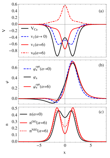
Figure 1: (a) Caticha potential, $V_{\rm Ca}(x;a,b)$, along with the effective potentials, $v_{0}$ and $v_{1}$, in the limit of vanishing interaction, $\alpha\rightarrow 0$, and for $\alpha=3$. For $\alpha\rightarrow 0$, only $v_{1}\neq 0$. Other parameters: $t_{0}=0.2$. (b)Non-interacting and optimized Wannier states for $\alpha\rightarrow 0$ and $\alpha=3$. (c) Ground state density (red lines) compared with the non-interacting density (black line). The solid and dotted lines show the density calculated with optimized and non-interacting orbitals, respectively.

For a contact interaction, the orbital optimization equations for the singlet state $|\Phi_{S}\rangle$, Eqs.(17-18), become local and they reduce to a set of coupled orbital-dependent single-particle Schrödinger equations with self-consistently defined external potentials. Specifically, setting $w(x-x^{\prime})=\alpha\,\delta(x-x^{\prime})$ and $\lambda=1$, for all $\alpha\neq 0$ we can write:

$$\hat{h}(x)\psi_{\mu}(x)+v_{\mu}(x)\psi_{\mu}(x)=\bar{\epsilon}_{\mu}\psi_{\mu}(x),\quad{\rm with}\,\mu=0,1$$ (30)

and

$$v_{0}=\alpha\!\left(\psi_{0}^{2}-\sqrt{\frac{\bar{\rho}_{1}}{\bar{\rho}_{0}}}\psi_{1}^{2}\right)\,\,{\rm and}\,\,v_{1}=\alpha\!\left(\psi_{1}^{2}-\sqrt{\frac{\bar{\rho}_{0}}{\bar{\rho}_{1}}}\psi_{0}^{2}\right).$$ (31)

We solve Eqs. (30-31) numerically. The results are also shown in Fig.1(a-c).

We remind that the above equations are for a singlet ground state. In the case of a triplet the interaction terms cancel in Eq. (27), (28), however since both orbitals are occupied the variational problem is well defined and its solution simply yields the bonding and anti-bonding eigenstates of the single-particle Hamiltonian. As a result, in the following,“optimized orbitals” (OO) always refer to the optimum orbitals for a singlet ground-state, while the bonding and anti-bonding eigenstates of the non interacting problem are called “non-interacting orbitals” (NIO). As mentioned, for the present contact interaction, they are also the optimized orbitals in the triplet subspace.

As discussed in Sec. IV.1.1 even for an infinitesimal interaction, the optimum $\psi_{1}$ differs from the non-interacting antibonding molecular eigenstate. It is interesting to obtain an expression for the potential determining $\psi_{1}$ in the weak coupling limit of Eq. 23,

$$v_{1}=-\frac{8t}{1-r_{ab}}\psi_{0}^{2},$$

were $r_{ab}=\int dx\phi_{a}^{2}\phi_{b}^{2}$. As we see in Fig. 1(a), in the presence of an infinitesimal interaction, the potential $v_{1}$ represented by the dashed blue line, essentially tends to confine the charge closer to the bond region. The corresponding optimum Wannier orbitals therefore shrink and shift toward the bond with a consequent sizable increase of the tunneling amplitude and of the Hubbard interaction, $U$ with respect to their values calculated starting from the non-interacting molecular eigenstates, as shown in Fig. 2(a) where we see that, even in the vanishing interaction limit, we have a finite renormalisation of $t$ and $U$.

At finite $\alpha$, the optimum orbitals $\psi_{0}$ and $\psi_{1}$ are respectively the ground and first excited state of the single-particle Hamiltonians defined by Eqs. (30-31). As shown by the dashed and solid red lines in Fig. 1(a), in this case, both $v_{0}$ and $v_{1}$ are roughly confined to the bond region and they have opposite characters, $v_{0}$ is repulsive while $v_{1}$ is attractive. $v_{0}$ becomes important going beyond the weak-coupling limit and its dominant effect is that it tends to reduce the weight of $\psi_{0}$ in the bond region and it leads to a suppression of the tunneling compensating the effect of $v_{1}$, see Fig.2(a).

The optimization of the orbitals not only affects the parameters of the lattice model but it also leads to different ground state densities when we go back to the continuum, this is what we show in Fig. 1(c). There we plot the density calculated with optimized and non-interacting orbitals, respectively $n^{\rm OO}=\bar{\rho}_{0}^{\rm OO}\psi_{0}^{2}+\bar{\rho}_{1}^{\rm OO}\psi_{1}^{2}$ and $n^{\rm NIO}=\bar{\rho}_{0}^{\rm NIO}\psi_{g}^{2}+\bar{\rho}_{1}^{\rm NIO}\psi_{u}^{2}$, along with the non-interacting density, $n_{0}=2\psi_{g}^{2}$ with $\psi_{g}$ and $\psi_{u}$ denoting the bonding and antibonding non-interacting orbitals and $\bar{\rho}_{\mu}^{\rm OO}$ and $\bar{\rho}_{\mu}^{\rm NIO}$ indicating respectively the elements of the one-body density matrix calculated with the optimized and with the non-interacting lattice parameters. We see that there is a substantial difference between the density in the three cases and that the optimization of the orbitals strongly reduces the bond charge. Furthermore by considering Fig.2(a), one can easily understand that orbital optimization generally tends to increase the ratio $U/t$ thus bringing the system in a more correlated state.

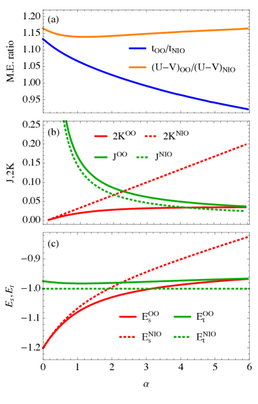
Figure 2: (a)Renormalization of the hopping amplitude and of $U-V$ as a function of $\alpha$ shown as ratio between the matrix element (M.E.) computed with optimized orbitals (OO) and non-interacting orbitals (NIO). (b) Direct and superexchange couplings as a function of $\alpha$ (c) Energy of the singlet and of the triplet as a function of $\alpha$. In both panels (b) and (c) solid and dotted lines indicate quantities calculated using optimized and non-interacting orbitals. Energies are in units of $I_{0}$.

V.1 Orbital optimization effects for excitation energies and the phase diagram

A major purpose of model Hamiltonians is to compute phase diagrams and excitation energies. For a periodic Mott insulating system one is interested in the magnetic Hamiltonian. It is customary to compute the magnetic parameters for a dimer and insert them in the many-site Heisenberg model.Anderson1950 Proceeding in this way the many-site Heisenberg model will have a ferromagnetic ground state when the dimer has a triplet ground state. Below we will show that the stability of the triplet state is very sensitive to the strategy used to obtain the model parameters with important implications for the description of ferromagnetism with model Hamiltonians.

Once the variational setting of this work is adopted for optimizing the orbitals the following problem appears. Since one can apply the variational principle in each subspace with well defined quantum numbers, if the orbitals depend on the state, in principle, one should optimize the orbitals in any such subspace, i.e. one should use different orbitals and parameters depending if one is computing the energy of the ground state or of an excited state with different quantum numbers (like the triplet in the present case). Not only this would be very cumbersome, but we will show below that such strategy leads to unphysical results. At least in the present case, we can show that, due to a cancellation of errors, the best strategy to compute the phase diagram and excitations energies is to compute the singlet and the triplet energies with the parameters optimized for the same singlet state.

Let us consider the effects of orbital optimization on the exchange energy defined as usual as the energy difference between triplet and singlet. For our simple toy-model the latter depends on the choice of the orbitals and it is in general given by:

$$E_{t}-E_{s}=\frac{\Delta_{{\rm U}}-U+V-4K}{2}-\Delta_{h}$$ (32)

where $\Delta_{h}=0$ if the singlet optimized orbitals are used for both the singlet and the triplet wave-functions and energies. Hereafter this choice will be dubbed “fixed singlet orbitals” (FSO). Another possibility is to use “state dependent orbitals” (SDO). In this case parameters for each state are computed with its own optimized orbitals and $\Delta_{h}$ accounts for the effects of orbital relaxation, i.e. $\Delta_{h}=2I_{0}+\bar{h}_{00}+\bar{h}_{11}$with the last two terms computed using the singlet optimized orbitals. In both cases, FSO and SDO, the Coulomb matrix elements appearing in Eq. (32) have to be calculated using the singlet-optimized orbitals since, for a contact interaction, the Coulomb matrix elements do not contribute to the triplet’s energy.

Notice that for FSO and assuming $U-V\gg t,\,K,\,t_{c}$, we recover the standard result that the exchange equals the sum of a kinetic and a Coulomb term and it is approximately given by:

$$E_{t}-E_{s} \sim \frac{2(t-t_{c})^{2}}{U-V}-K=J/2-K.$$ (33)

where we indicated as $J$ the super-exchange interaction, $J=4(t-t_{c})^{2}/(U-V)$. Thus, for sufficiently large direct exchange the ground state becomes a triplet.

In Fig. 2b we show the effects of orbital optimization on $J$ and $K$ as a function of $\alpha$ for the optimized orbitals assuming the singlet ground state (OO). We also show the result for non-interacting orbitals (NIO) which coincides with the parameters that would be obtained for the triplet ground state.

As one can see, while the changes in $J$ are small or moderate $K$ is strongly renormalized by orbital optimization in the singlet state. In particular, while in the absence of orbital optimization $K$ grows linearly with $\alpha$, in the presence of singlet orbital optimization it tends to saturate.

A spurious singlet to triplet transition is found for $\alpha\sim 2$ if the parameters are computed with the widely used approximation of taking non-interacting orbitals. This is also what we see in Fig. 2c where we plot the energy of the singlet and triplet as a function of $\alpha$.

The transition is shifted to a larger value $\alpha\sim 3$ if one adopts the SDO strategy and computes the ground state energy (panel c, full red line for the singlet and dashed green line for the triplet). A much improved result is obtained if the FSO strategy is applied (full lines in panel c). In this case the transition disappears from our studied window and singlet and triplet become degenerate at strong coupling as expected from the exact solution.girardeau1960 In this approximation one can use a fixed model Hamiltonian to compute ground state and excited states as customary done which is obviously a great simplification.

In these regards let us remark that in the limit $\alpha\rightarrow\infty$, $|\phi_{S}\rangle$ does not represent the lowest energy singlet, indeed it can be shown by means of the so-called Girardeau mappinggirardeau1960 that the correct singlet ground-state should have the form:

$$|\Phi_{S,\infty}\rangle=|\psi_{0}({\bf r}_{1})\psi_{1}({\bf r}_{2})-\psi_{1}({\bf r}_{1})\psi_{0}({\bf r}_{2})|.$$ (34)

This state is degenerate with the triplet and it lies outside the space of our trial wave-functions, that is essentially restricted to the all the states that can be expressed as the sum of Slater determinants constructed with the optimized orbitals. More precisely, the state $|\Phi_{S,\infty}\rangle$ has a non-analytic behavior at ${\bf r}_{2}={\bf r}_{1}$, which could be described only by an infinite sum of Slater determinants and cannot be captured by the our trial wavefunction. Indeed, our trial wave-function is just the best variational state within the restricted basis and contains only two Slater determinants [Eq. (13)]. The situation is different for the triplet state which for the spatial part reads,

$$|\Phi_{T,\alpha}\rangle=\psi_{0}({\bf r}_{1})\psi_{1}({\bf r}_{2})-\psi_{1}({\bf r}_{1})\psi_{0}({\bf r}_{2}).$$ (35)

This state coincides with our trial triplet state and is the exact ground state for all values of $\alpha$ in the triplet subspace. The triplet energy $E_{t}=-I_{0}$ appearing in Fig. 2c is the exact triplet energy and also the asymptotic ground state energy for $\alpha\rightarrow\infty$ were the triplet and the singlet become degenerate.

All the spurious transitions reported above are rooted in the fact that the variational state yields the exact ground state energy for the triplet and a variational upper bound energy for the singlet. When computing energy differences errors do not cancel and the triplet is spuriously favored. A similar problem arises in lattice Hamiltonians when trying to describe ferromagnetism.Gunther2011

Using the FSO strategy the same systematic error is incurred in the computation of the ground state energy of the triplet and the singlet so that the error cancels in the excitation energy and a physically correct value is obtained. Thus, for example, the spin wave spectrum will be physically meaningful for a Heisenberg model with parameters computed within the FSO scheme while it will give a generally wrong result if orbital relaxation is neglected or if the SDO strategy is adopted to compute an effective exchange energy. The price to pay is that a spurious shift appears in the total energy of the system however this shift is irrelevant to compute most physical properties with the model Hamiltonian.

VI Gutzwiller natural orbital functional

As we discussed so far, for a two-site molecule the structure of the one- and two-body density matrices, $D$ and $\rho$, appearing in Eqs. (10) is exactly known. This allowed us to write the energy as a functional of a single parameter $\gamma$, which determines the lattice ground-state, and of the orbitals $\{\varphi_{i}\}$, see Eq. (16).

In very rough terms, the logic behind Gutzwiller Ansatz can be summarized by the following statement: a lattice system with a repulsive Hubbard interaction should have a smaller doubly occupancy probability than a non-interacting one. The variational Gutzwiller wave function for the lattice model can be written as,gutzwiller1963 ; gebhard2009 ; Vollhardt1984 ; Metzner1987 ; Gebhard1990

$$|\Phi_{\gamma}\rangle=\frac{\gamma^{D}}{C^{1/2}_{\gamma}}|\Phi_{0}\rangle$$ (36)

where $|\Phi_{0}\rangle$ is a Slater determinant, $D=\sum_{i}n_{i\uparrow}n_{i\downarrow}$ counts the total double occupancy, $\gamma$ is a variational parameter and $C_{\gamma}=\langle\Phi_{0}|\gamma^{2D}|\Phi_{0}\rangle$ a normalization constant. In the two-site case this equation simply gives the exact lattice ground-state of Eq. (13).

The projector $\gamma^{D}$ reduces the weights of the configurations with doubly occupied sites and the optimization of $\gamma$ essentially coincides with the optimization of the average double occupancy.

A somewhat complementary point of view is adopted in RDMFT helbig2007 ; buijse2002 ; gritsenko2005 ; lathiotakis2009 ; goedecker1998 ; sharma2008 ; sharma2013 where the fundamental variational object is the whole one-body density matrixgilbert1975 defined by its eigenstates and the corresponding eigenvalues as

$$\Gamma({\bf r},{\bf r}^{\prime})=\sum_{n}\phi^{*}_{n}({\bf r})\phi_{n}({\bf r}^{\prime})\bar{\rho}_{n}.$$ (37)

Since within Gutzwiller approach $\gamma$ completely determines, through $q$, the full one-body density matrix on the lattice, one may “eliminate” $\gamma$ in favor of $q$ and extend Gutzwiller theory to the continuum by constructing a RDMFT which reduces to standard Gutzwiller theory when the single particle basis is kept fixed but which determines the orbitals variationally in the general case. In the following, we show how the above reasoning applies to the two-site system.

In the two-site case, starting from the lattice Gutzwiller wave-function Eq. (13), it is straightforward to obtain the corresponding one- and two-body density matrices in terms of the bonding and antibonding orbitals, $\psi_{0}$ and $\psi_{1}$, and of their occupancies. We indeed have for the one-body density matrix

$$\Gamma_{1}^{\rm G}({\bf r},{\bf r}^{\prime}) = \sum_{\sigma}\langle\Phi_{\gamma}|\Psi^{\dagger}_{\sigma}({\bf r})\Psi_{\sigma}({\bf r}^{\prime})|\Phi_{\gamma}\rangle$$

$$= (1+q)\psi_{0}({\bf r})\psi_{0}({\bf r}^{\prime})+(1-q)\psi_{1}({\bf r})\psi_{1}({\bf r}^{\prime})$$

where $q=2\gamma/C_{\gamma}$ while for the diagonal part of the two-body density we obtain:

$$\Gamma^{\rm G}_{2}({\bf r},{\bf r}^{\prime})=\sum_{\sigma\sigma^{\prime}}\langle\Phi_{\gamma}|\Psi_{\sigma^{\prime}}^{\dagger}({\bf r}^{\prime})\Psi_{\sigma}^{\dagger}({\bf r})\Psi_{\sigma}({\bf r})\Psi_{\sigma^{\prime}}({\bf r}^{\prime})|\Phi_{\gamma}\rangle$$

$$=\left(\sqrt{1+q}\,\psi_{0}({\bf r})\psi_{0}({\bf r}^{\prime})-\sqrt{1-q}\,\psi_{1}({\bf r})\psi_{1}({\bf r}^{\prime})\right)^{2}.$$ (39)

By direct comparison we easily see that, in a “minimal” basis consisting of just two orbitals, $\Gamma^{\rm G}_{2}({\bf r},{\bf r}^{\prime})$ coincides with the exact two-body density for a two-fermion closed-shell system first obtained by Löwdin and Shull (LS)lowdin1956 . Equations (VI) and (VI) therefore show that for a two-site molecule Gutzwiller theory just gives the LS density matrix functional in a restricted basis. More explicitly by replacing Eqs. (VI-VI) in the well-known expression of the energy in terms of the one- and two- body density matrices, one can easily show that the following relation holds

$$E[\Gamma^{\rm G}_{1},\Gamma^{\rm G}_{2}]\! = \!\!\!\int\!d{\bf r^{\prime}}\lim_{\bf r\rightarrow\bf r^{\prime}}\left[\hat{h}_{\bf r}\Gamma^{\rm G}_{1}({\bf r},{\bf r}^{\prime})\right]+\!$$

$$\!\!\!\!\!\!\!\!\!\!\!\!+ \!\!\!\!\!\!\!\!\!\!\!\!\frac{1}{2}\!\int\!\Gamma^{\rm G}_{2}({\bf r},{\bf r}^{\prime})w({\bf r},{\bf r}^{\prime})d{\bf r}d{\bf r^{\prime}}=E_{\rm 2site}[\psi_{0},\psi_{1},\gamma],$$

i.e. one recovers Eq. (16) obtaining a natural orbitals Gutzwiller functional. Since Gutzwiller theory captures many aspects of correlated systems this suggest that RDMFT may indeed be a promising root to tread materials in which correlations dominate.

VII Conclusions

In this work we have shown how to determine the optimum basis orbitals to expand a single-band Hubbard-like lattice model starting from a continuum Hamiltonian. The method can be seen as a multiconfigurational generalization of the Hartree-Fock method where the solution of the lattice Hamiltonian provides the configurations that are included in the wave-function and the OLMO equations provide the analogy of the Hartree-Fock equations for the orbitals. In the case in which only one Slater determinant is retained in the lattice wave-function the OLMO equations reduce to the Hartree-Fock equations for the orbitals as these are the optimum orbitals for a single Slater determinant. In the general case, the ground state can be seen as a variational wave function where both the orbitals and the weight of the different Slater determinants are optimized.

As explained above, differently from previous works [marzari2012, ; paul2006, ] aimed at constructing the optimum Wannier orbitals for a given truncated lattice Hamiltionian starting from a fixed single-particle subspace, here we do not make any a priori assumption on the lattice model and we leave full variational freedom to the orbitals in order to consider the optimization of the single-particle subspace that will be used to construct the lattice model. The procedure requires the simultaneous determination of the lattice ground-state and the solution of the OLMO continuum equations. Therefore, the optimum orbitals generally depend on the lattice ground-state and viceversa.

The OLMO equations are quite hard to solve in general thus, it is of great interest to clarify, at least in one test-ground case, what the effect of orbital optimization would be. By solving the OLMO equations for a toy-model with two delta-function-interacting fermions in a one dimensional two-well potential, we demonstrate that orbital optimization:

• induces qualitative and quantitative modifications of the parameters of the lattice model;

• may affect significantly the ground-state of the system and excitation energies;

• in the infinitesimal interaction limit yields orbitals and parameters that differ substantially from the non-interacting ones.

As regards point (i) we have shown in particular that orbital optimization tends to increase the ratio $U/t$ while it strongly quenches the direct exchange coupling $K$ with dramatic implications for the stability of a ferromagnetic state.

As regards point (ii) we have shown that orbital optimization carried on “blindly” for any state, leads to wrong excitation energies and a wrong phase diagram since the variational Ansatz has not the same quality for all states. In our case it is exact for a triplet state with only contact interactions among fermions and it is only approximate for singlet states. Therefore, errors do not cancel when computing excitation energies or the phase diagram. For Coulomb or other interactions which are large at short distances we expect a similar state-dependent quality of the variational state. For example on a single band system of electrons the exchange hole will reduce much more the Coulomb interaction energy in the case of the fully polarized state than in the paramagnetic state. Thus the paramagnetic state is a harder problem for the effective variational wave-function and the same problem will arise.

We have shown that the best strategy is to choose one reference state and use the same parameters for all states. The reference state, in our case, is the singlet state but would be a paramagnetic state in the case of many atoms. Then the orbitals and parameters in the model are fixed for all states. This is reassuring for lattice model methods which usually assume a fixed orbital in the model rather than changing the orbital (and the Hamiltonian parameters for each state). On the other hand, we have found that for some parameters like the direct exchange energy, neglecting orbital optimization leads to gross errors so the choice of the reference state is also crucial.

Unfortunately, there is no a general rule to choose what state to use as a reference state without knowing a priori the ground state of the system. However, a good guess can be obtained by computing the total energy in competing states. We see from Fig. 2c that there is a modest worsening of the energy by computing the triplet energy with singlet orbitals and the error depends weakly on the coupling. On the contrary, computing the singlet energy with the orbitals optimized for the triplet (NIO) leads to an error (evaluated as difference with the best singlet variational state) that diverges at strong coupling. Such an analysis clearly suggests that the singlet reference state is the best compromise for all states of the system, as we indeed find, and can be used as a guideline in more complicated situations.

Another problem in a more general context is how to solve, at least approximately, the OLMO equations in many orbital cases. One possibility is to use some approximate but accurate lattice solver like dynamical mean-field theory or a Gutzwiller variational wave-function for the lattice problem and insert the many-body correlations in the OLMO equations for the orbitals and iterate until convergence. In this context, it is interesting that in the case of two-electrons the variational problem can be mapped to a reduced density matrix functional theory which establish a connection between this emerging method of continuous approaches and the Gutzwiller method, popular in the lattice Hamiltonian community. Clearly it would be worth exploring how far such connection can be pushed in extended systems. On the other hand, the link with Gutzwiller theory puts the RDMFT in a framework which is known to give a good description of the physics of strongly correlated systems.

References

- (1) J. Slater and W. Shockley, Phys. Rev. 50, 705 (1936).
- (2) J. Frenkel, Phys. Rev. 37, 17 (1931).
- (3) G. Wannier, Phys. Rev. 52, 191 (1937).
- (4) J. Hubbard, Proc. R. Soc. London. A. 276, 238 (1963).
- (5) J. Kanamori, Prog. Theor. Phys. 30, 275 (1963).
- (6) M. Gutzwiller, Phys. Rev. Lett. 10, 159 (1963).
- (7) S. Boys, Rev. Mod. Phys. 32, 296 (1960).
- (8) J. Foster and S. Boys, Rev. Mod. Phys. 32, 300 (1960).
- (9) C. Edmiston and K. Ruedenberg, Rev. Mod. Phys. 35, 457 (1963).
- (10) N. Marzari, A. A. Mostofi, J. R. Yates, I. Souza, and D. Vanderbilt, Rev. Mod. Phys. 84, 1419 (2012).
- (11) A. Chiesa, S. Carretta, P. Santini, G. Amoretti, and E. Pavarini, Phys. Rev. Lett. 110, (2013).
- (12) M. Greiner, O. Mandel, T. Esslinger, T. W. Hänsch, and I. Bloch, Nature 415, 39 (2002).
- (13) M. Lewenstein, A. Sanpera, V. Ahufinger, B. Damski, A. S. De, and U. Sen, Advances in Physics 56, 243 (2007).
- (14) Z.-J. Ying, M. Liu, H.-G. Luo, H.-Q. Lin, and J. Q. You, Phys. Rev. A 92, 053823 (2015).
- (15) M. Liu, Z.-J. Ying, J.-H. An, and H.-G. Luo, New J. Phys. 17, 043001 (2015).
- (16) I. Paul and G. Kotliar, Eur. Phys. J. B 51, 189 (2006).
- (17) W. Kohn and L. J. Sham, Phys. Rev.140, A1133 (1965).
- (18) J. Spaelek, R. Podsiady, W. Wójcik, and A. Rycerz, Phys. Rev. B 61, 15676 (2000).
- (19) J. Kurzyk, W. Wojcik, and J. Spaelek, Eur. Phys. J. B 66, 385–398 (2008).
- (20) A. P. Kadzielawa, J. Spalek, J. Kurzyk, and W. Wójcik, Eur. Phys. J. B 86, (2013).
- (21) Z.-J. Ying, V. Brosco, G. Lopez, D. Varsano, P. Gori-Giorgi, and J. Lorenzana, Phys. Rev. B 94, 075154 (2016).
- (22) V. I. Anisimov, F. Aryasetiawan, and A. I. Lichtenstein, J. Phys.: Condens. Matter 9, 767 (1997).
- (23) V. I. Anisimov, A. I. Poteryaev, M. A. Korotin, A. O. Anokhin, and G. Kotliar, J. Phys.: Condens. Matter 9, 7359 (1997).
- (24) A. Lichtenstein and M. Katsnelson, Phys. Rev. B 57, 6884 (1998).
- (25) G. Kotliar, S. Savrasov, K. Haule, V. Oudovenko, O. Parcollet, and C. Marianetti, Rev. Mod. Phys. 78, 865 (2006).
- (26) J.-P. Julien and J. Bouchet, Phys. B Condens. Matter 359, 783 (2005).
- (27) G.-T. Wang, X. Dai, and Z. Fang, Phys. Rev. Lett. 101, 066403 (2008).
- (28) K. Ho, J. Schmalian, and C. Wang, Phys. Rev. B 77, 073101 (2008).
- (29) X. Deng, L. Wang, X. Dai, and Z. Fang, Phys. Rev. B 79, 075114 (2009).
- (30) T. Schickling, J. Bünemann, F. Gebhard, and W. Weber, New J. Phys. 16, 093034 (2014).
- (31) J. E. Hirsch and S. Tang, Phys. Rev. B 40, 2179 (1989).
- (32) N. Helbig, N. Lathiotakis, M. Albrecht, and E. Gross, Europhys. Lett. 77, 67003 (2007).
- (33) M. Buijse and E. Baerends, Molecular Physics 100, 401 (2002).
- (34) O. Gritsenko, K. Pernal, and E. J. Baerends, J. Chem. Phys. 122, 204102 (2005).
- (35) N. Lathiotakis, S. Sharma, J. Dewhurst, F. Eich, M. Marques, and E. Gross, Phys. Rev. A 79, 040501 (2009).
- (36) S. Goedecker and C. Umrigar, Phys. Rev. Lett. 81, 866 (1998).
- (37) S. Sharma, J. Dewhurst, N. Lathiotakis, and E. Gross, Phys. Rev. B 78, 201103 (2008).
- (38) S. Sharma, J. Dewhurst, S. Shallcross, and E. Gross, Phys. Rev. Lett. 110, (2013).
- (39) T. Gilbert, Phys. Rev. B 12, 2111 (1975).
- (40) F. Gebhard and M. Gutzwiller, 4, 7288 (2009).
- (41) S. Murmann, A. Bergschneider, V. M. Klinkhamer, G. Zorn, T. Lompe, and S. Jochim, Phys. Rev. Lett. 114, 080402 (2015).
- (42) A. Caticha, Phys. Rev. A 51, 4264 (1995).
- (43) F. Cooper, A. Khare, and U. Sukhatme, Physics Reports 251, 267 (1995).
- (44) L. D. Landau and Lifshitz, in Quantum Mechanics: Non-Relativistic Theory. Vol. 3 (3rd ed.)., edited by P. Press (1977).
- (45) N. Helbig, I. V. Tokatly, and A. Rubio, The Journal of Chemical Physics 131, 224105 (2009).
- (46) P. W. Anderson, Phys. Rev. 79, 350 (1950).
- (47) M. Girardeau, Journal of Mathematical Physics 1, 516 (1960).
- (48) F. Günther, G. Seibold, and J. Lorenzana, Phys. Status Solidi 248, 339 (2011).
- (49) D. Vollhardt, Rev. Mod. Phys. 56, 99 (1984).
- (50) W. Metzner and D. Vollhardt, Phys. Rev. Lett. 59, 121 (1987).
- (51) F. Gebhard, Phys. Rev. B 41, 9452 (1990).
- (52) P.-O. Löwdin and H. Shull, Phys. Rev. 101, 1730 (1956).