Polaron spin echo envelope modulations in an organic semiconducting polymer

Abstract

Theoretical treatment of the electron spin echo envelope modulation (ESEEM) spectra from polarons in a semiconducting $\pi$- conjugated polymer is presented. The contact hyperfine coupling and the dipolar interaction between the polaron and proton spins are found to have distinct contributions in the ESEEM spectra. However, since the two contributions are spaced very closely, and the dipolar contribution is dominant, the detection of the contact hyperfine interaction is difficult. To resolve this problem, a recipe of probing the contact hyperfine and dipolar interactions selectively is proposed, and a method for detecting the polaron contact hyperfine interaction is formulated. The ESEEM decay due to the polaron random hopping is analyzed, and the robustness of the method against this decay is verified. Moreover, this decay is linked to the transport properties of polarons, providing an auxiliary probe for the polaron transport.

I Introduction

Over the past decades, semiconducting organic $\pi$- conjugated small molecule and polymer materials have been become widely used in optoelectronic devices such as light-emitting diodes and solar cells. Forrest04 ; SpecIss07 This triggered an increasing interest in the area of organic electronics, uncovering a variety of new concepts. Remarkably, it was established that the charge carrier spin is fundamental to electrical and optical properties of organic semiconductors. However, because of the extremely complex nature, many important aspects of the spin dynamics and underlying microscopic mechanisms are not yet well understood. This includes the microscopic structure of charge-carrier polaron states, and the resulting hyperfine coupling of polaron spin to the local magnetic environment, which is a key for understanding the spin-dependent processes in organic semiconductors.

Optically and electrically detected magnetic resonance (ODMR and EDMR, respectively) are highly efficient spectroscopic tools for the investigation of microscopic properties of organic semiconductors. Shinar While the conventional electron spin resonance (ESR) techniques measure the spin polarization, ODMR and EDMR probe optically and electrically active paramagnetic states, Cavenett81 ; Street82 ; Depinna82 which are crucial to many organic semiconductor applications. Moreover, as the spin polarization in organic semiconductors is typically low, ODMR and EDMR are much more sensitive than the conventional ESR. Stutzmann00 ; Lifshitz04 ; McCamey06

Substantial progress in this direction was made by the pulsed EDMR (pEDMR) experiments. Dane08 ; DanePRL10 ; DanePRB10 ; Behrendes10 ; BoehmePRL12 ; Malissa ; Kipp15 Unlike the continuous wave measurements, these experiments are capable of probing the coherent spin dynamics, and thus provide a closer view on the spin-dependent processes. Importantly, pEDMR (and pODMR) offer the implementation of various spin-echo based spectroscopic techniques in the study of organic semiconductors. BoehmePRL12 ; Malissa This motivates the present theoretical study of a spectroscopic method based on the two-pulse (Hahn) echo and three-pulse echo sequences. Slichter

In many organic semiconductors the spin-orbital coupling is very week, and the polaron spin dynamics is governed mainly by the hyperfine interaction of polaron spin with the surrounding proton spins. Dediu09 ; ThoNatMat Therefore, probing the polaron hyperfine interaction is very important. A magnetic resonance technique widely used to investigate the hyperfine interaction of paramagnetic centers is electron spin echo envelope modulation (ESEEM) spectroscopy. DT ; SchJ The pEDMR implementation of this technique, applied to organic polymer poly[2-methoxy-5-(2^′-ethyl-hexyloxy)- 1,4-phenylene vinylene] (MEH-PPV), was recently reported by Malissa et al. Malissa Employing a version of ESEEM, the authors of Ref. Malissa, have been able to resolve the proton spectral line in MEH-PPV and that of the deuteron and proton in partially deuterated MEH-PPV.

In this paper we develop a theory of ESE modulations based on the two-pulse, primary echo, and three-pulse, stimulated echo (primary and stimulated ESEEM, respectively), in application to MEH-PPV. We argue that the spectral lines observed in Ref. Malissa, are due to the magnetic dipolar coupling of polaron spin with the distant protons, while the protons coupled to the polaron spin with the contact hyperfine interaction (HFI) are not detected. Our theory offers a way to address the distant and the contact hyperfine protons selectively, by a proper choice of the stimulated ESEEM parameters. Thus we propose a method of probing the contact HFI. This also gives a valuable information on the polaron orbital state, stipulating the contact HFI.

The paper is organized as follows. In the next Section we discuss the hyperfine interaction between the polaron and proton spins, particularly in polymer poly[p-phenylene vinylene] (PPV) and its derivative, MEH-PPV. The derivation of ESEEM is given in Section III. In Section IV we analyze the effect of random orientations of polymer chains. The polaron hopping and the resulting ESE modulation decay is considered in Section V. We discuss our results in Section VI. Appendices contain the details of our analytical and numerical calculations.

II Polaron spin in a $\pi$- conjugated organic semiconducting material

In organic materials, polarons reside on certain molecular or polymer sites and hop between the sites. While residing on a site a polaron spin, $\mathbf{S}$, interacts with $N$ surrounding hydrogen nuclear spins, $\mathbf{I}_{j}=1/2$, $j=1,..,N$. In a strong static magnetic field, $\mathbf{B}_{0}=B_{0}\hat{\mathbf{z}}$, this spin dynamics can be described by the Hamiltonian,

$$H=\Omega S^{z}+\sum_{j=1}^{N}S^{z}\bigl{(}A_{j}I^{z}_{j}+B_{j}I^{x}_{j}\bigr{)}-\omega_{I}\sum_{j=1}^{N}I^{z}_{j},$$ (1)

where $\Omega=\gamma_{e}\hbar B_{0}$ and $\omega_{I}=\gamma_{n}\hbar B_{0}$ are the polaron and nuclear Larmor frequencies, and $\{A_{j}\}$, $\{B_{j}\}$ are the hyperfine coupling constants. This (pseudo)secular description Slichter implies that $B_{0}$ greatly exceeds the local magnetic fields created by the nuclear magnetic moments, i.e., $\Omega\gg\omega_{\text{hf}}$, where $\omega_{\text{hf}}=\frac{1}{2}\sqrt{\sum_{j}(A_{j}^{2}+B_{j}^{2})}$ is the average polaron precession frequency in the local field of surrounding nuclear spins. Assuming measurements in the X – band, BoehmePRL12 ; Malissa we will take $B_{0}\approx 345$ mT and $\omega_{I}/2\pi\approx 14.7$ MHz.

The coupling constants in Eq. (1) depend on the relative orientation of $\mathbf{B}_{0}$ and the polaron host molecular or polymer site. Typically, organic semiconductors are amorphous materials lacking any long range order in molecular or polymer orientations. Thus, the coupling constants $\{A_{j},B_{j}\}$ differ from site to site, even if the sites have the same microscopic structure.

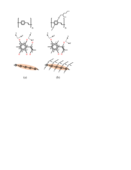
Figure 1: (Color online) Conjugated polymer PPV (a) and its derivative, MEH-PPV (b). Upper and middle panels: chemical structures and unit cells. The principal $x$, $y$ axes of the C–H proton hyperfine tensors at B and C^′ carbon sites are different from those at B^′, C, E, and F carbon sites, while the $z$ axes are the same and perpendicular to the plane of the picture (in MEH-PPV there are no C–H protons at B^′ and C sites). Lower panels: half-widths of the spatial extents of polarons (brown ovals), according to Ref. Kuroda2000, .

Polarons in conjugated polymer PPV and MEH-PPV

The hyperfine interaction between the polaron and proton spins is determined by the chemical structure of host molecule or polymer, which also governs the orbital state of the polaron. To be specific, we focus on polymer PPV and its derivative, MEH-PPV (see Fig. 1). We base our consideration on the picture of polaron wavefunction and underlying proton hyperfine coupling to the polaron spin advocated in Refs. Kuroda94PRL, ; Kuroda95, ; KurodaSSC95, ; Kuroda2000, ; for a comprehensive review, see Ref. Kuroda2003, .

Protons can be naturally divided into two groups. The first group includes protons located within the envelope of polaron spin distribution, thus contributing to the contact hyperfine interaction. These are all C–H protons covalently coupled to the polymer backbone carbons, where the polaron wavefunction resides. Because of an exponentially fast spatial decay the polaron wavefunction covers a finite number of protons. As it is discussed below, in PPV and MEH-PPV this number is order of few tens. So we neglect contact protons coupled to the polaron spin weaker than 0.5 MHz; the number of such contact protons is small, and their overall effect is inessential.

Distant protons, which form the second group, couple to a polaron spin with a magnetic dipolar interaction. These protons belong both to polymer backbones and substituent side-groups. Simple estimates show that nearly every distant proton couples to a polaron spin with less than 1 MHz strength. However, because of the slow, $\propto 1/r^{3}$ decay of the dipolar interaction the effective number of these protons is order of few thousand, so that their overall effect can be noticeable.

II.0.1 Contact hyperfine interaction

The polaron spin, $\mathbf{S}$, couples to a C–H proton spin, $\mathbf{I}$, by the hyperfine interaction $\mathbf{S}\cdot\rho_{\text{S}}\hat{\mathbf{A}}\cdot\mathbf{I}$, where $\rho_{\text{S}}$ is the polaron spin density on the carbon $p\pi$ orbital and $\hat{\mathbf{A}}$ is the hyperfine tensor. Thus the polaron contact hyperfine interaction is completely described in terms of $\hat{\mathbf{A}}$ and $\rho_{\text{S}}$.

From the analysis of unpaired carbon orbital states it is established Morton that the principal $x$ and $z$ axes of the hyperfine tensor are parallel to the C–H bond and the $p\pi$ orbital axes, respectively (see Fig. 1). Principal elements of the hyperfine tensor are approximately expressed as

$$\bigl{(}A_{x},A_{y},A_{z}\bigr{)}=-\bigl{(}[1-\alpha]A_{H},[1+\alpha]A_{H},A_{H}\bigr{)},$$ (2)

where $A_{H}/2\pi=60$ to $80$ MHz is the McConnell’s constant, and $\alpha=0.5$ to $0.6$ is the degree of anisotropy. Morton

Equation (2) is quite general for organic $\pi$-electron radicals. For PPV and MEH-PPV, experimental studies are conforming with $A_{H}/2\pi=70$ MHz and $\alpha=0.5$. Kuroda94PRL ; Kuroda95 ; Kuroda2000 These numerical values are used in our calculations. The remaining necessary ingredient for describing the polaron contact hyperfine interaction is the polaron spin density at the carbon sites, $\rho_{\text{S}}$. In our subsequent calculations we employ the spin density presented in Table 1. This form is found from a model calculation KurodaSSC95 and verified by the analysis of spectral lineshapes in ENDOR Kuroda94PRL ; Kuroda95 and light-induced ESR Kuroda2000 experiments.

Formally, $\rho_{\text{S}}$ in Table 1 is calculated for PPV. However, the same data can be used for spin densities in other PPV derivatives, Kuroda2000 particularly in MEH-PPV, thus neglecting the effect of substituent groups on $\rho_{\text{S}}$ to the leading order.

Table 1: Spin density of a polaron in PPV chain, $\rho_{\text{S}}$, taken from Ref. KurodaSSC95, . Small values, $|\rho_{\text{S}}|<0.01$, are neglected. The site assignment corresponds to that of Fig. 1. The unit cell at the polaron center is denoted by $0$, thereby the unit cells with significant values of $\rho_{\text{S}}$ range from $-3$ to $3$.

site $\!\!\backslash\!\!$ cell	-3	-2	-1	0	1	2	3
$A$	–	0.01	0.04	0.08	0.04	–	–
$B$	–	0.01	-0.015	0.035	-0.005	0.03	-0.005
$B^{\prime}$	–	0.01	-0.015	0.04	–	0.03	–
$C$	–	–	0.03	–	0.04	-0.015	0.01
$C^{\prime}$	–	-0.005	0.03	-0.005	0.035	-0.015	0.01
$D$	–	–	–	0.04	0.08	0.04	0.01
$E$	0.01	-0.01	0.09	0.08	–	0.035	–
$F$	–	0.035	–	0.08	0.09	-0.01	0.01

We further restrict ourselves on MEH-PPV. According to Table 1 and Fig. 1, in MEH-PPV there are $N_{c}=22$ contact proton spins coupled to a polaron spin at sites $B$, $C^{\prime}$, $E$, and $F$, over 7 consecutive unit cells that the polaron spin distribution covers (note that in MEH-PPV the C–H protons at carbon sites B and C^′ are replaced by substituent groups). In the Hamiltonian (1) we label the contact protons by $j=1,..,N_{c}$. The coupling constants $\{A_{j},B_{j}\}_{j=1}^{N_{c}}$ depend on the relative orientations of the corresponding C–H bonds and the applied magnetic field, $\mathbf{B}_{0}=B_{0}\hat{\mathbf{z}}$. We denote the components of $\hat{\mathbf{z}}$ in the principal basis of the $j$- th hyperfine tensor by $q_{\mu j}$, $\mu=x$, $y$, $z$. The coupling constants are related to the hyperfine tensor elements Eq. (2) as

$$A_{j}=\rho_{\text{S}}(j)\!\sum_{\mu}A_{\mu}q_{\mu j}^{2},\quad A_{j}^{2}+B_{j}^{2}=\rho_{\text{S}}^{2}(j)\!\sum_{\mu}A_{\mu}^{2}q_{\mu j}^{2}.$$ (3)

For each $j$, $\rho_{\text{S}}(j)$ is given in Table 1, and $q_{\mu j}$ can be found for any direction of $\mathbf{B}_{0}$ from the description of principal hyperfine axes in Fig. 1. Thus finding the coupling constants and performing the orientation averaging of different quantities of interest becomes a straightforward numerical task. As the first step we calculate the average local frequency due to the contact hyperfine coupling,

$$\omega_{\text{hf},c}=\left\langle\frac{1}{2}\sqrt{\sum_{j\leq N_{c}}\bigl{(}A_{j}^{2}+B_{j}^{2}\bigr{)}}\right\rangle\approx 2\pi\times 7.25\,\text{MHz}.$$ (4)

The corresponding ESR line would be Gaussian, with the full width at half maximum of $6.1$ G, in agreement with Ref. Kuroda2000, .

II.0.2 Interaction with the distant protons

Distant protons couple to the polaron local spin density via magnetic dipolar interaction. The strength of this interaction is determined by the material morphology, including the molecular packing and the average density of protons. Relying upon the reported data on the molecular packing Claes01 ; Kilina13 ; Qin13 and van der Waals radii of hydrogen and carbon Bondi64 ; Motoc85 ; Spillane92 , we restrict the minimal distance between the polymer backbone carbons and distant protons to $d_{\text{min}}=2.2$ Å. Furthermore, based on the MEH-PPV mass density, $1$ g/mL, Kilina13 ; Qin13 and its chemical structure in Fig. 1, we infer the average proton density, 55 nm^-3. Except in the regions restricted by $d_{\text{min}}$ around a polymer chain, we take random distributions of protons with this average density. We also employ point dipolar coupling between a distant proton and each of the 38 non-zero polaron spin densities, given in Table 1. Thus, in the applied magnetic field, $\mathbf{B}_{0}=B_{0}\hat{\mathbf{z}}$, a distant proton couples to the polaron spin with the Hamiltonian (1), where

$$A=\hbar\,\gamma_{e}\gamma_{n}\sum_{l=1}^{38}\rho_{\text{S}}(l)\frac{1-3\cos^{2}\theta_{l}}{R_{l}^{3}},$$

$$B=\hbar\,\gamma_{e}\gamma_{n}\sum_{l=1}^{38}\rho_{\text{S}}(l)\frac{3\sin\theta_{l}\cos\theta_{l}}{R_{l}^{3}}.$$ (5)

Here, $\rho_{\text{S}}(l)$ is the polaron spin density at the carbon site $l$, $\mathbf{R}_{l}$ is the vector connecting the distant proton to this carbon site, and $\theta_{l}$ is the angle between $\mathbf{R}_{l}$ and $\mathbf{B}_{0}$.

Equations (II.0.2) give coupling constants of a single distant proton. A large number of distant protons is included numerically, by sampling realizations of their spacial distributions. In our simulations of various quantities of interest the results converge for about $N_{d}=2000$ uniformly distributed distant protons and do not change appreciably if this number is increased by an order of magnitude. This is because we deal with spatial integrals of $\sim A^{2},B^{2}$, and their combinations, which vanish $\propto R^{-6}$ or faster, and thus converge quickly. Averaging over the random orientations of polymer chains should be performed additionally, as the polaron spin density is not spherically symmetric and different chain orientations are inequivalent.

For the average local frequency from the distant protons this yields $\omega_{\text{hf},d}\approx 2\pi\times 2$ MHz, leading to the the total average local frequency,

$$\omega_{\text{hf}}=\left\langle\frac{1}{2}\sqrt{\sum_{\text{all }j}\bigl{(}A_{j}^{2}+B_{j}^{2}\bigr{)}}\right\rangle\approx 2\pi\times 7.52\,\text{MHz}.$$ (6)

From Eqs. (4) and (6) it is seen that, on average, the distant protons are responsible only for a small fraction of the local hyperfine field. Yet they have a strong effect on the fine structure of ESEEM, as will be seen shortly.

In theoretical studies of spin dynamics in organic semiconductors a semiclassical approach SchulWol is often used. While this approach does not capture the fine structure of the ESEEM signal, it provides a convenient way for the characterization of the signal decay. In the semiclassical treatment, the nuclear spin dynamics given by the last term of Eq. (1) is ignored, and the on-site hyperfine interaction is replaced by a random local static magnetic field felt by a polaron spin. SchulWol Accordingly, the on-site semiclassical Hamiltonian in the secular approximation reads:

$$H_{SC}=\bigl{(}\Omega+\omega_{z})S^{z},$$ (7)

where $\omega_{z}$ is random and uncorrelated from site to site. This random frequency is often described by a Gaussian distribution. In the case under consideration the Gaussian distribution of frequencies should be taken with the standard deviation, $\omega_{\text{hf}}$. Note that the distribution of random fields resulting from a magnetic dipolar bath of randomly spaced spins is rather Lorentzian, with a certain frequency cutoff. Abragam In our case this is pertinent to the contribution of distant protons. However, a relatively short cutoff and overall small contribution of distant protons in $\omega_{\text{hf}}$ ensure that the Gaussian distribution of local frequencies is accurate also in our case.

III Spin echo with ideal pulses

Generally, electron spin echo envelope modulation (ESEEM) spectroscopy is used to investigate the hyperfine interactions of paramagnetic species. DT To set a framework for discussing the application of spin echo experiments in organic semiconductors we give a treatment of the ESEEM originating from the two-pulse, Hahn echo sequence, Fig. 2(a) (primary ESEEM), and the three-pulse sequence, Fig. 2(b) (stimulated ESEEM). In Fig. 2, $\pi/2$ and $\pi$ denote the rotation angle of spins along the $x$-axis in the rotating frame, induced by resonant microwave pulses, whereas $\tau$ and $T$ are the free evolution periods between the pulses. The pulses are assumed to be ideal. Depending on $\tau$ and $T$ the echo amplitude undergoes modulations, which we denote by $E(2\tau)$ for the primary ESEEM and $E(\tau,T)$ for the stimulated ESEEM.

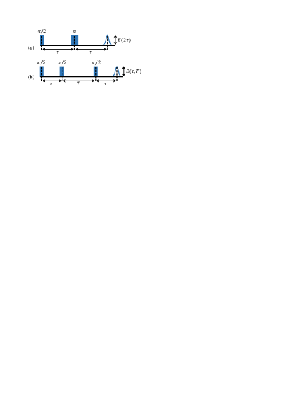
Figure 2: (Color online) ESEEM pulse sequences considered in the text. (a) Primary ESEEM. (b) Stimulated ESEEM.

Using the density matrix formalism, the (normalized) modulation functions can be written as

$$E(2\tau)=-2\,\text{Tr}\left[U(\tau)\hat{\rho}(0)U^{\dagger}(\tau)S^{y}\right],$$ (8)

$$E(\tau,T)=-2\,\text{Tr}\left[U(\tau,T)\hat{\rho}(0)U^{\dagger}(\tau,T)S^{y}\right],$$ (9)

where $\hat{\rho}(0)$ is the density operator before the first pulse, and the evolution operators are given by

$$U(\tau)=e^{-i\tau H}\bigl{[}\pi\bigr{]}e^{-i\tau H}\bigl{[}\pi/2\bigr{]},$$

$$U(\tau,T)=e^{-i\tau H}\bigl{[}\pi/2\bigr{]}e^{-iTH}\bigl{[}\pi/2\bigr{]}e^{-i\tau H}\bigl{[}\pi/2\bigr{]},$$

in which $[\phi]=\exp(i\phi S^{x})$ is the rotation operator for an ideal pulse with flip angle $\phi$, and $H$ is the Hamiltonian, Eq. (1). For our further purposes we consider the initial density operator, $\hat{\rho}(0)=(1/2+S^{z})\otimes\rho_{I}$, formally describing a polaron spin ensemble polarized along the $z$-axis. At the same time we neglect the thermally-induced polarization of the nuclear spin ensemble and take the nuclear density operator proportional to the unity, $\rho_{I}\propto\mathbf{1}$. The explicit calculation of modulation functions is facilitated by the fact that the Hamiltonian, Eq. (1), preserves the $z$-component of polaron spin. One gets DT

$$E(2\tau)=\prod_{j=1}^{N}\!\!\left(1-2k_{j}\sin^{2}\frac{\omega_{j+}\tau}{2}\sin^{2}\frac{\omega_{j-}\tau}{2}\right)$$ (10)

for the primary ESEEM and

$$E(\tau,T)=\frac{1}{2}\prod_{j=1}^{N}\!\!\left(1-2k_{j}\sin^{2}\frac{\omega_{j+}[\tau+T]}{2}\sin^{2}\frac{\omega_{j-}\tau}{2}\right)$$

$$+\frac{1}{2}\prod_{j=1}^{N}\!\!\left(1-2k_{j}\sin^{2}\frac{\omega_{j+}\tau}{2}\sin^{2}\frac{\omega_{j-}[\tau+T]}{2}\right)\quad$$ (11)

for the stimulated ESEEM, where the frequencies,

$$\omega_{j\pm}=\left[(\omega_{I}\pm A_{j}/2)^{2}+B_{j}^{2}/4\right]^{1/2},$$ (12)

are the nuclear spin level splittings due to the external magnetic field and the hyperfine coupling to the polaron spin in either up or down state, and

$$k_{j}=\left[\frac{\omega_{I}B_{j}}{\omega_{j+}\omega_{j-}}\right]^{2}$$ (13)

are the modulation depths. The primary ESEEM formula (10) is a product of the factors from individual nuclei. This is the consequence of the polaron spins being in a coherent superposition of up and down states during the evolution periods. In the stimulated ESEEM, during the evolution time $T$ the polaron spins are in a definite state, up or down, leading to the first and the second products in Eq. (III), respectively.

Two major factors influencing modulation signals Eqs. (10) and (III) in a real experiment are the orientation disorder of polymer chains and the polaron random hopping between the sites. In the next two Sections we address the effects of these factors.

IV The effect of orientation disorder

The samples in typical experiments on organic polymers are disordered films, and the observed signals incorporate contributions from all orientations of polymer chains. Therefore we average Eqs. (10) and (III) over random orientations of polymer chains, and consider the disorder-averaged modulation signals, $\langle E(2\tau)\rangle$, $\langle E(\tau,T)\rangle$, together with their spectra given by the cosine Fourier transforms, ftnt $\tilde{E}(\omega)=\mathcal{F}_{\tau}[\langle E(2\tau)\rangle]$, $\tilde{E}(\tau,\omega)=\mathcal{F}_{T}[\langle E(\tau,T)\rangle]$.

IV.1 Orientation-averaged primary ESEEM

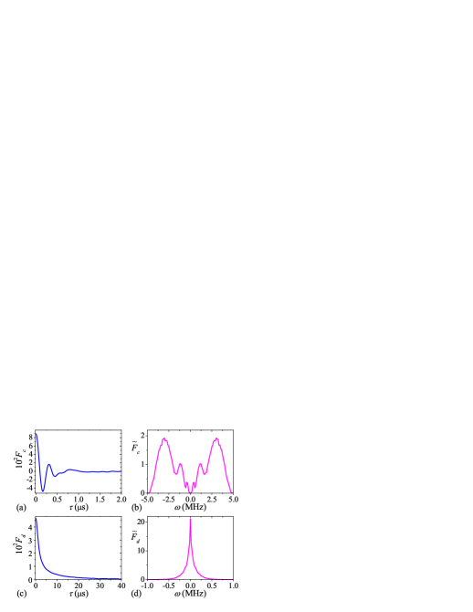
Figure 3: (Color online) Functions $F_{c}(\tau)$ and $F_{d}(\tau)$, introduced in Eqs. (17) and (18) respectively, are plotted with blue. (b) and (d): The respective cosine Fourier transforms, $\tilde{F}_{c}(\omega)$ and $\tilde{F}_{d}(\omega)$, are plotted with magenta, in the same units.

The HFI described above leads to small values of modulation depths, $k_{j}\ll 1$. Moreover, the sum of all modulations depths, $\kappa=\sum k_{j}$, is also small. This alludes to expanding Eq. (10) over small $k_{j}$ (for more details on this approach see Appendix A). We write:

$$E(2\tau)=1-\frac{1}{2}\sum_{j}k_{j}\biggl{[}1-\cos(\omega_{j+}\tau)-\cos(\omega_{j-}\tau)$$

$$\left.+\frac{1}{2}\cos\bigl{(}[\omega_{j+}-\omega_{j-}]\tau\bigr{)}+\frac{1}{2}\cos\bigl{(}[\omega_{j+}+\omega_{j-}]\tau\bigr{)}\right]\!.$$ (14)

Equation (IV.1) shows that the primary ESEEM spectrum involves four groups of carrier frequencies, $\{\omega_{j\pm}\}$ and $\{\omega_{j+}\pm\omega_{j-}\}$. We subsequently use the approximation,

$$\omega_{j\pm}\approx\omega_{I}\pm A_{j}/2.$$ (15)

For the distant protons Eq. (15) follows from the weak coupling, $A_{j},B_{j}\ll\omega_{I}$. For the contact protons with a stronger coupling Eq. (15) is valid due to the weak anisotropy of the contact HFI, see Appendix A. Employing Eq. (15) the four frequency groups involved are $\{|A_{j}|\}$, $\{\omega_{I}-|A_{j}|/2\}$, $\{\omega_{I}+|A_{j}|/2\}$, and $2\omega_{I}$. The relation, ftnt2 $\omega_{I}>\frac{3}{2}|A_{j}|$, ensures that $\{|A_{j}|\}$ carries the low-frequency modulations, resolved from the higher frequency groups. Besides, the second and the third groups are close to $\omega_{I}$, mirroring each other about this frequency.

Another conclusion from Eq. (IV.1) is that the contributions of the contact and the distant protons in $E(2\tau)$ are simply additive. We separate these contributions by introducing the notations, $E_{c}(2\tau)$ and $E_{d}(2\tau)$, respectively. More specifically, $E_{c}(2\tau)$ is the partial sum of the first $N_{c}$ terms in Eq. (IV.1), whereas $E_{d}(2\tau)$ is that of the terms with $j>N_{c}$, and thus $E(2\tau)=1+E_{c}(2\tau)+E_{d}(2\tau)$. Using Eq. (15) in Eq. (IV.1) and averaging the result over the disorder in polymer chain orientations yields:

$$\langle E_{\beta}(2\tau)\rangle=-\frac{\langle\kappa_{\beta}\rangle}{2}-\frac{1}{4}F_{\beta}(2\tau)-\frac{\langle\kappa_{\beta}\rangle}{4}\cos(2\omega_{I}\tau)$$

$$+F_{\beta}(\tau)\cos(\omega_{I}\tau),$$ (16)

where the subscript, $\beta=c,d$, refers to the contact and the distant protons, respectively, and the partial sums

$$F_{c}(\tau)=\left\langle\sum\nolimits_{j\leq N_{c}}k_{j}\cos(A_{j}\tau/2)\right\rangle,$$ (17)

$$F_{d}(\tau)=\left\langle\sum\nolimits_{j>N_{c}}k_{j}\cos(A_{j}\tau/2)\right\rangle,$$ (18)

$\kappa_{c}=\langle\sum_{j=1}^{N_{c}}k_{j}\rangle$, and $\kappa_{d}=\langle\sum_{j>N_{c}}k_{j}\rangle$ are introduced. Equation (IV.1) gives the orientation-averaged ESE modulation function in terms of $F_{c}(\tau)$ and $F_{d}(\tau)$. Particularly, the low-frequency modulations are included in the second term of Eq. (IV.1). The third term of Eq. (IV.1) describes oscillations of a constant amplitude on the frequency $2\omega_{I}$, both for the contact and the distant protons. Finally, modulations with the frequencies close to $\omega_{I}$ are incorporated in the last term of Eq. (IV.1).

First we elaborate on the contribution of distant protons. On the timescale, $\tau\sim 1/\omega_{I}$, the function $F_{d}(\tau)$, Fig. 3(c), varies only slightly. Thus the last term of $\langle E_{d}(2\tau)\rangle$ in Eq. (IV.1) can be viewed as oscillations with the frequency, $\omega_{I}$, and the envelope, $F_{d}(\tau)$. The cosine Fourier transform, $\tilde{F}_{d}(\omega)$, plotted in Fig. 3(d), is a sharp peak at $\omega=0$. Through this function the cosine Fourier spectrum of the distant protons is found. It involves three well-resolved peaks; a dip of the form, $-\frac{1}{4}\tilde{F}_{d}(\omega/2)$, near the origin, a sharp peak at $\omega_{I}$ of the shape, $\tilde{F}_{d}(\omega-\omega_{I})$, and a sharper, negative $\delta$- peak at $2\omega_{I}$.

In the case of the contact proton contribution, the function $F_{c}(\tau)$, Fig. 3(a), changes considerably on the timescale, $\tau\sim 1/\omega_{I}$, because of the presence of large $A_{j}\sim\omega_{I}$. Therefore the last term of $\langle E_{c}(2\tau)\rangle$ in Eq. (IV.1) does not admit a simple interpretation in terms of the oscillations with the frequency $\omega_{I}$ and a smooth envelope. Its cosine Fourier transform, $\tilde{F}_{c}(\omega-\omega_{I})$, incorporates two bands mirroring each other about $\omega_{I}$, as can be inferred from Fig. 3(b). These bands come from the modes with frequencies, $\{\omega_{I}\pm|A|_{j}/2\}_{j=1}^{N_{c}}$, spread by the orientation disorder. Except for these two bands and the negative $\delta$- peak at $2\omega_{I}$, the cosine Fourier spectrum of the contact protons involves a low-frequency band of the form, $-\frac{1}{4}\tilde{F}_{c}(\omega/2)$, originating from the frequencies $\{|A|_{j}\}_{j=1}^{N_{c}}$.

Figure 4 plots the primary ESEEM spectrum, $\tilde{E}(\omega)$, calculated from Eq. (10) by a Monte Carlo sampling of the polymer chain orientations, employing Eqs. (3), (II.0.2). Its structure near $\omega_{I}=14.7$ MHz includes a sharp peak at $\omega_{I}$ and two wider side-bands mirroring each other about $\omega_{I}$. Based on the above analysis we identify the side-bands with the contribution of contact protons and the sharp peak with that of the distant protons. Thus, the forms of the side-bands and the sharp peak are given by $\tilde{F}_{c}(\omega-\omega_{I})$ and $\tilde{F}_{d}(\omega-\omega_{I})$, respectively. This identification is clearly confirmed in Fig. 4(b) where we plot the contributions of contact and distant protons separately.

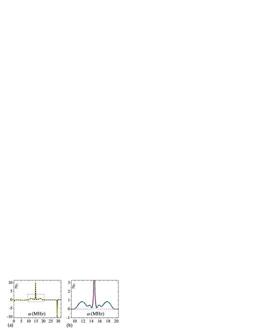
Figure 4: (Color online) The primary ESEEM spectrum $\tilde{E}$, calculated from orientation disorder averaged Eq. (10) numerically, is plotted in black. (a): The cosine Fourier transform of the sum, $\langle E_{c}(2\tau)\rangle+\langle E_{d}(2\tau)\rangle$, is plotted with yellow dashed line, from Eq. (IV.1). (b): Zoom in of the region indicated in the left panel with a rectangle. $\tilde{F}_{c}(\omega-\omega_{I})$ and $\tilde{F}_{d}(\omega-\omega_{I})$ are plotted with the cyan and magenta dotted lines, respectively. It is seen that the spectral peak at $\omega_{I}=14.7$ MHz is exclusively due to the distant protons, whereas the side bands come from the contact protons.

IV.2 Orientation-averaged stimulated ESEEM

The stimulated ESEEM can be analyzed along the same lines. Expanding Eq. (III) over small $k_{j}$ and keeping the leading terms, one gets:

$$E(\tau,T)=1-\sum_{j}\frac{k_{j}}{2}\Bigl{[}\sin^{2}\frac{\omega_{j+}\tau}{2}\bigl{(}1-\cos\omega_{j-}[\tau+T]\bigr{)}$$

$$+\sin^{2}\frac{\omega_{j-}\tau}{2}\bigl{(}1-\cos\omega_{j+}[\tau+T]\bigr{)}\Bigr{]}.\qquad$$ (19)

Thus the stimulated ESEEM spectrum involves only two groups of frequencies, $\{\omega_{j+}\}$ and $\{\omega_{j-}\}$. Our subsequent analysis employs the approximation Eq. (15). By separating the contact and the distant proton contributions in Eq. (IV.2) and averaging over the polymer chain orientations we get $\langle E(\tau,T)\rangle=1+\langle E_{c}(\tau,T)\rangle+\langle E_{d}(\tau,T)\rangle$, where the $T$- dependent parts of $\langle E_{\beta}(\tau,T)\rangle$, $\beta=c,d$, are

$$\langle E_{\beta}(\tau,T)\rangle\simeq\frac{1}{2}F_{\beta}(\tau+T)\cos(\omega_{I}[\tau+T])$$ (20)

$$-\frac{1}{4}F_{\beta}(T)\cos(\omega_{I}[2\tau+T])-\frac{1}{4}F_{\beta}(2\tau+T)\cos(\omega_{I}T).$$

As a function of $T$, $\langle E_{d}(\tau,T)\rangle$ modulates only with the proton Zeeman frequency, $\omega_{I}$, and its cosine Fourier transform, ftnt $\tilde{E}_{d}(\tau,\omega)$, is basically a sharp peak around that frequency. Predictions about the $\tau$- dependence of the modulation strength can be made even without performing the disorder averaging. Indeed, Eq. (IV.2) shows that the modulation amplitude is reduced if $\tau$- values are possible such that $\sin(\omega_{j\pm}\tau/2)\approx 0$ for all protons. Since for the distant protons all $\omega_{j\pm}$ are close to $\omega_{I}$, one can expect a reduction of the modulation amplitude of $\langle E_{d}(\tau,T)\rangle$ at the $\tau$- values with $\sin(\omega_{I}\tau/2)=0$. Similarly, one can anticipate an increase of modulation amplitude at the $\tau$- values with $\sin(\omega_{I}\tau/2)=\pm 1$.

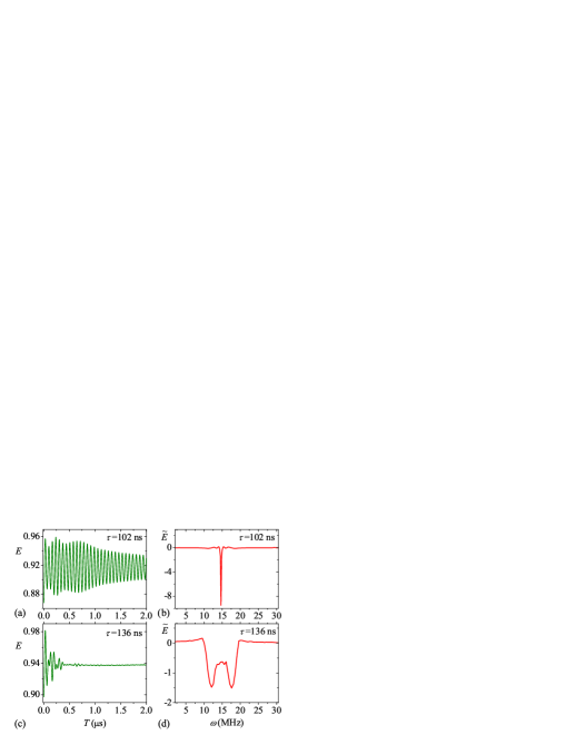
Figure 5: (Color online) The stimulated ESEEM $\langle E(\tau_{n},T)\rangle$, calculated from orientation disorder averaged Eq. (III) numerically, is plotted against $T$ at fixed $\tau_{n}=(\pi/\omega_{I})n$ for $n=3,\,\tau_{3}\approx 102$ ns (a), and $n=4,\,\tau_{4}\approx 136$ ns (c). The corresponding spectra $\tilde{E}(\tau_{n},\omega)$, $n=3$ (b) and $n=4$ (d), are plotted against $\omega$. The strong reduction of the peak at $\omega_{I}=14.7$ MHz for even $n$, allowing the observation of the contact proton hyperfine coupling, is obvious.

In Appendix A we prove that the $T$- modulation amplitude of $\langle E_{d}(\tau,T)\rangle$ is reduced at the $\tau$- values, $\tau_{n}=(\pi/\omega_{I})n$ with even integer $n$, and increased at those with odd integer $n$. We also show that, for $n\leq 30$, the decrease in the amplitude of $\langle E_{d}(\tau_{n},T)\rangle$ between odd $n$ and even $n$ is more than two orders of magnitude for small $n$ and more than 15 times for large $n$. Note that this includes all $\tau_{n}$ within the interval, $0<\tau<1\,\mu$s, which covers the experimentally available $\tau$- domain, taking into account the decay of the signal in a real experiment.

The $T$- modulation of $\langle E_{c}(\tau,T)\rangle$, given by Eq. (20), cannot be interpreted as having a single frequency $\omega_{I}$, because the function $F_{c}$ varies abruptly on the timescale, $T\sim 1/\omega_{I}$. Similar to that of the primary modulation, its cosine Fourier transform, ftnt $\tilde{E}_{c}(\tau,\omega)$, represents two bands near $\omega_{I}$. However, in this case these bands are not quite symmetric around $\omega_{I}$. Importantly, $\tau=\tau_{n}$ are not critical for $\langle E_{c}(\tau,T)\rangle$ and there is no special reduction at even $n$, as it is shown in Appendix A.

Summarizing, measurements of the stimulated ESEEM spectra at $\tau=\tau_{n}$ with odd $n$ encounter a strong peak at $\omega_{I}$, which in a real situation could make the observation of weaker contact proton sidebands difficult. On the other hand, reduction of the peak occurs at $\tau=\tau_{n}$, while the contribution of the contact protons is preserved. This constitutes a basis of the method for addressing the distant and the contact hyperfine protons selectively, by choosing appropriate $\tau$- values and analyzing the $T$-dependence of the stimulated ESEEM.

To illustrate the method, in Fig. 5 we plot the time-domain signals $\langle E(\tau_{n},T)\rangle$ and their spectra for $n=3$ and $n=4$, calculated from orientation-averaged exact equation (III) numerically. Spectral plots in Figs. 5(b) and (d) demonstrate the suppression of the peak at $\omega_{I}=14.7$ MHz when changing $n$ from odd to even.

V Echo modulations of hopping polarons

The polaron random walk leads to the decay of ESEEM, thus imposing limitations on the observability of modulations. On the other hand, this decay can serve as a probe for understanding the aspects of polaron transport. In this Section we investigate the ESEEM of polarons performing random walk over orientationally disordered polymer sites and coupling to the nuclear spins according to Eq. (1). Our main goal is to reveal the hopping regimes where the ESEEM signal, and particularly the contact hyperfine spectrum, is not distorted.

The spin dynamics of a randomly hopping polaron is dependent on the polaron random walk dimensionality. MD15 ; RR14 ; CzK ; MLD Its analytical description is the simplest in 3D, where the approximation neglecting the self-intersections of the random walk trajectories is good. This is equivalent to the strong collision approximation which provides a simple way of describing the spin relaxation of a randomly hopping carrier. Kubo79

The multiple trapping model Hartenstein96 ; Jakobs93 ; HarmonPRL13 ; HarmonPRB14 is an implementation of the strong collision approximation, often used to explain the transport in organic materials Coropceanu07 and particularly in PPV and its derivatives. Blom00 We base our consideration on the multiple trapping model. Within this model the polaron hopping from a polymer site, $\mathbf{r}$, is described by the rate,

$$W_{\mathbf{r}}=\nu\exp\bigl{[}\varepsilon_{\mathbf{r}}/k_{B}T\bigr{]},$$ (21)

where $\nu$ is the hopping attempt frequency, $\varepsilon_{\mathbf{r}}$ is the trapping energy at the site $\mathbf{r}$, $k_{B}$ is the Boltzmann constant, and $T$ is the temperature. The trapping energies are all negative and random, with the exponential distribution, $\mathcal{N}(\varepsilon)\propto\exp\bigl{[}\varepsilon/k_{B}T_{0}\bigr{]}$. Hence the model is defined by two parameters, $\nu$ and the dispersion parameter, $\alpha\equiv T/T_{0}$. In the high-temperature or shallow-trap limit, $\alpha\to\infty$, the hopping rates are uniform and the waiting time statistics of the polaron random walk is governed by the Poisson distribution, $P(t)=\nu\exp(-\nu t)$. For finite $\alpha$ this distribution assumes the algebraic form, $P(t)\propto t^{-1-\alpha}$, reflecting the broad distribution of hopping rates.

V.1 Primary ESEEM of hopping polarons

The generalization of Eq. (10) for hopping polarons and the evaluation of the resulting echo modulation function, $\mathcal{E}(2\tau)$, is described in Appendix B. We calculate $\mathcal{E}(2\tau)$ by Monte-Carlo sampling of the random-walk trajectories over the orientation disordered polymer sites. But before turning to our results on $\mathcal{E}(2\tau)$ we introduce the echo modulation function of hopping carriers calculated from the semiclassical Hamiltonian (7), $\mathcal{E}_{\text{SC}}(2\tau)$, which is the semiclassical counterpart of $\mathcal{E}(2\tau)$.

$\mathcal{E}_{\text{SC}}(2\tau)$ is a non-oscillatory, monotonously decreasing function of the delay time $\tau$. In the high-temperature limit, $\alpha\to\infty$, the perturbative treatment over small $\eta\equiv\nu/\omega_{\text{hf}}\ll 1$ given in Appendix C yields

$$\mathcal{E}_{\text{SC}}(2\tau)=\left[1+\eta\sqrt{\pi}\,\text{erf}(\omega_{\text{hf}}\,\tau)\right]\!e^{-2\nu\tau},$$ (22)

where $\text{erf}(x)$ is the error function. For $\tau>2/\omega_{\text{hf}}$ the error function in Eq. (22) changes very little, so that $\mathcal{E}_{\text{SC}}(2\tau)$ assumes the exponential form, $\mathcal{E}_{\text{SC}}(2\tau)\propto\exp(-2\tau/T_{2})$, with the decoherence time, $T_{2}=1/\nu$. The decay of $\mathcal{E}_{\text{SC}}(2\tau)$ with $\tau$ is exponential also in the fast hopping regime, $\eta\gg 1$. However, due to the motional narrowing, the dependence of $T_{2}$ on $\nu$ in this regime is reversed; $T_{2}=\nu/\omega_{\text{hf}}^{2}$. Combining the two forms, we write:

$$T_{2}=1/\nu+\nu/\omega_{\text{hf}}^{2}.$$ (23)

Even though the decay of $\mathcal{E}_{\text{SC}}(2\tau)$ in the intermediate regime $\eta\sim 1$ is not exponential, the dephasing time Eq. (23) gives the correct timescale for that decay too.

Our numerical simulations show that with decreasing $\alpha$ the decay of $\mathcal{E}_{\text{SC}}(2\tau)$ becomes slower and non-exponential, with a progressively stronger long-time tail. For $\eta\ll 1$ this can be explained as follows. The dependence of $\mathcal{E}_{\text{SC}}(2\tau)$ on $\alpha$ is stipulated by the number of deep traps, which grows with decreasing $\alpha$. A trapped polaron is subject to a static hyperfine magnetic field. Because the echo pulse sequence eliminates the dephasing caused by static field components, Abragam ; Slichter the decay of $\mathcal{E}_{\text{SC}}(2\tau)$ becomes slower with the increasing fraction of trapped polarons. The effect is most pronounced at long times due to the slow, algebraic decrease of the waiting time distribution, resulting in the overall non-exponential dephasing of $\mathcal{E}_{\text{SC}}(2\tau)$.

The dependence of $\mathcal{E}_{\text{SC}}(2\tau)$ on $\alpha$ for $\eta\gg 1$ is less transparent. Nevertheless, the non-exponential character of $\mathcal{E}_{\text{SC}}(2\tau)$ at finite $\alpha$, observed in our numerical simulations, is established analytically also for this case. YMR

Summarizing, the exponential behavior of $\mathcal{E}_{\text{SC}}(2\tau)$ is a signature of the uniform hopping rates with either fast or slow hopping (i.e., away from $\eta\sim 1$), whereas in all the remaining situations $\mathcal{E}_{\text{SC}}(2\tau)$ is non-exponential.

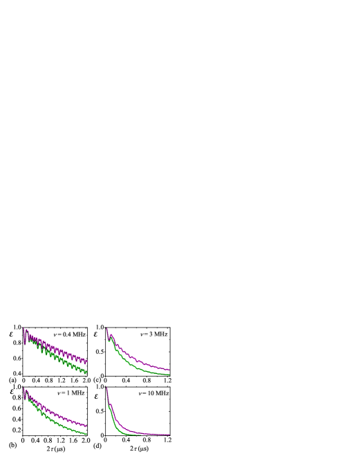
Figure 6: (Color online) The decay of echo modulation for slow polaron hopping, $\eta\equiv\nu/\omega_{\text{hf}}\ll 1$. The right-hand sides of Eq. (24) are plotted for $\alpha\equiv T/T_{0}\gg 1$ (green), and $\alpha=2$ (magenta). The corresponding left-hand sides are plotted with black dotted lines. The hopping attempt frequencies and corresponding values of $\eta$ are: $\nu=0.4$ MHz, $\eta=0.0085$ (a), $\nu=1$ MHz, $\eta=0.021$ (b), $\nu=3$ MHz, $\eta=0.063$ (c), and $\nu=10$ MHz, $\eta=0.21$ (d). The plots clearly confirm the validity of Eq. (24).

The analysis of $\mathcal{E}(2\tau)$ reveals different types of $\tau$- dependence in slow ($\eta\ll 1$) and fast ($\eta\gg 1$) hopping regimes. In the slow hopping regime, where this dependence is more complex, we numerically find that $\mathcal{E}(2\tau)$ is quite accurately quantified by

$$\mathcal{E}(2\tau)=\langle E(2\tau)\rangle\mathcal{E}_{\text{SC}}(2\tau),$$ (24)

where $\langle E(2\tau)\rangle$ is established in the previous Section. To substantiate this relation, in Fig. 6 we plot $\mathcal{E}(2\tau)$ numerically calculated for four different small values of $\eta$, and compare them with the curves resulting from Eq. (24). The plots confirm the validity of Eq. (24) for the hopping attempt frequencies up to $\eta=0.21$.

Equation (24) suggests that the fine structure of $\mathcal{E}(2\tau)$ is totally described by $\langle E(2\tau)\rangle$, whereas its decay is given by $\mathcal{E}_{\text{SC}}(2\tau)$. Important to us is the question whether the decay destroys any information on the spectrum of contact HFI, enclosed in $\langle E(2\tau)\rangle$, i.e., in $\langle E_{c}(2\tau)\rangle$. The answer is found from Fig. 3(a), indicating that $F_{c}(\tau)$ almost disappears for $\tau>1\,\mu$s. Thus, one is able to capture the complete spectrum if $\mathcal{E}(2\tau)$ is detectable for $\tau\leq 1\,\mu$s. Assuming that $\mathcal{E}(2\tau)\geq 0.05\,\mathcal{E}(0)$ is the restriction for the observation time, we find that for $\alpha\to\infty$ the contact HFI spectrum is not distorted if $\nu\leq 1.5$ MHz. At the same time, from Fig. 3(a) one can see that $F_{c}(\tau)$ is essentially non-zero for $\tau\leq 0.5\,\mu$s, meaning that the basic spectral features are detectable for $\nu\leq 3$ MHz.

For $\alpha\to\infty$ and larger $\nu$ the signal decay is faster and the spectrum distortion is progressively stronger. Furthermore, in the regime of fast hopping, $\eta\gg 1$, the fine structure of $\mathcal{E}(2\tau)$ is completely destroyed, even though the signal decays slower because of the motional narrowing. Instead of Eq. (24), here we get

$$\mathcal{E}(2\tau)=\mathcal{E}_{\text{SC}}(2\tau).$$ (25)

Therefore, for $\nu>3$ MHz low-temperature (small-$\alpha$) measurements can be crucial for the assessment of the primary ESEEM spectrum.

The experiment Ref. BoehmePRL12, confirms that the primary echo signal in MEH-PPV decays exponentially, for at least $T\geq 10$ K. This experiment does not address the fine structure of $\mathcal{E}(2\tau)$. However, the results of Ref. BoehmePRL12, suggest a uniform polaron hopping; $\alpha\gg 1$. At $T=10$ K the hopping rate is estimated to be $\nu\approx 1.64$ MHz, whereas at $T=295$ K it is $\nu\approx 2.87$ MHz. This refers to the slow hopping regime, where the ESEEM fine structure is shown to be observable.

V.2 Stimulated ESEEM of hopping polarons

The stimulated ESEEM of an ensemble of hopping polarons, $\mathcal{E}(\tau,T)$, is treated in the same way. We introduce its semiclassical counterpart, $\mathcal{E}_{\text{SC}}(\tau,T)$, and determine its $T$- dependence. Unlike the above analysis, however, here we restrict ourselves to the hopping regime, $\eta<1$, relevant for MEH-PPV.

In the high-temperature limit, $\alpha\to\infty$, we find the simple exponential decay,

$$\mathcal{E}_{\text{SC}}(\tau,T)=\mathcal{E}_{\text{SC}}(2\tau)\exp(-\nu T).$$ (26)

For finite $\alpha$ this decay slows down and becomes non-exponential. Similar to the primary ESEEM, the fine structure of the stimulated ESEEM is accurately described by the relation,

$$\mathcal{E}(\tau,T)=\langle E(\tau,T)\rangle\mathcal{E}_{\text{SC}}(\tau,T),$$ (27)

with $\langle E(\tau,T)\rangle$ characterized in the previous Section.

The same question as to whether the decay destroys any information enclosed in $\langle E(\tau,T)\rangle$ on the contact HFI, i.e., in $\langle E_{c}(\tau,T)\rangle$, should be answered in this case. The question is relevant for stimulated ESEEM measurements aimed at the detection of the contact HFI, which imply $\tau=(\pi/\omega_{I})n$ with even $n$. The answer is found from Eqs. (26), (27), and the fact that the amplitude of $\langle E_{c}(\tau_{n},T)\rangle$ is very small for $T>0.5\,\mu$s and nearly vanishing for $T>0.75\,\mu$s (see Appendix A). Assuming that the observation time is restricted by $\mathcal{E}(\tau_{n},T)\geq 0.05\,\mathcal{E}(\tau_{n},0)$, for $\alpha\gg 1$ the complete contact HFI spectrum of the stimulated ESEEM is detectable for $\nu\leq 4$ MHz, while its essential spectral features are preserved for $\nu\leq 6$ MHz. These limits are less restrictive than those on the primary ESEEM also because the decay of $\mathcal{E}_{\text{SC}}(\tau,T)$ with $T$ is twice slower than that of $\mathcal{E}_{\text{SC}}(2\tau)$ with $\tau$, cf. Eqs. (22) and (26).

VI Concluding remarks

We have studied the ESEEM spectroscopy of polarons in polymer MEH-PPV. As a reference, we adopted the microscopic picture of the polaron orbital state and its hyperfine interaction with the surrounding protons, established in ENDOR and light-induced ESR experiments. Kuroda94PRL ; Kuroda95 ; Kuroda2000 Our study incorporates the random orientations of polymer chains and the polaron random hopping. The resulting ESEEM spectra have distinct features from the polaron spin interaction with the distant protons and from that of the contact protons, which are intrinsic to the polaron. Utilizing the stimulated ESEEM we formulate a method which makes the separate observation of the interaction with the contact protons feasible, by properly choosing the time parameters.

Electrical or optical detection of any magnetic resonance relies upon the phenomenon of spin-dependent charge carrier recombination and transport. Since the work of Kaplan, Solomon, and Mott, KSM the explanation of this phenomenon in terms of weakly coupled polaron spin pairs is standard. Accordingly, pEDMR based ESEEM studies should include a weak polaron-polaron spin coupling. The perturbatively established effect of polaron pair spin coupling on ESEEM ZH consists in the partial shifts of modulation frequencies, $\delta\omega_{\pm}\approx\pm(J+D)^{2}/\omega_{I}$, where $J$ and $D$ are the strengths of the polaron pair spin exchange and dipolar couplings, respectively. In the case of MEH-PPV remote polaron pairs it is reasonable to neglect the spin exchange. As for the dipolar coupling, its contribution can be neglected if $D^{2}/\omega_{I}\ll\omega_{I}$. In the adopted model of polaron this condition is met for the polaron separation greater than 2 nm. In our consideration we neglected the effect of polaron-polaron spin coupling, assuming such large inter-polaron distances.

In a conventional ESR experiment the echo modulation is subject to a relaxation decay due to, e. g., electron-nuclear, spin-lattice, and dipole-dipole interactions. In addition to these, in pulsed ODMR and EDMR experiments various recombination-dissociation processes can also contribute in the ESEEM decay. However, the decay timescales measured so far Dane08 ; BoehmePRL12 ; Kipp15 point that the polaron hopping yields the fastest channel of decay. We address the destructive effect of the polaron hopping and determine the hopping regimes where the ESEEM spectral features are not distorted. Based on the experiment Ref. BoehmePRL12, we conclude that the polaron hopping in MEH-PPV is within this regime and our method is viable.

A pulsed EDMR study of the stimulated ESEEM spectrum of polarons in MEH-PPV was recently reported. Malissa Apparently, the working point in Ref. Malissa, is such that the spectral peak from the distant protons is strongly dominant. We believe that choosing the parameters as proposed above can lead to the detection of contact hyperfine spectrum, within the same experimental setup.

Our theory provides the means for further adjustments to the adopted picture of MEH-PPV polaron hyperfine interaction and transport properties, provided measurements according to the proposed method are available. Moreover, the theory can be straightforwardly generalized for organic materials lacking coherent charge transport, other than MEH-PPV.

Appendix A

In this Appendix we describe the details of the theoretical framework for the analysis in Section IV. Particularly, we address the disorder-averaged time-domain modulation signals $\langle E(2\tau)\rangle$, $\langle E(\tau,T)\rangle$, and their spectral functions, $\tilde{E}(\omega)$ and $\tilde{E}(\tau,\omega)$, in line with Ref. DT, .

In real experiments, as well as during numerical simulations, time-domain signals are found at discrete values of time. Typically, one obtains an array of values, $f(t_{k})$, for equidistant time points, $t_{k}=k\Delta t$, $k=0,1,..,L$. For the spectral analysis of such a signal it is convenient to introduce the discrete cosine Fourier transform, $\mathcal{F}_{t}[f(t)](\omega)\equiv\tilde{f}(\omega)$, as

$$\tilde{f}(\omega_{j})=\sum_{k=0}^{L}2f(t_{k})\cos(\omega_{j}t_{k})-f(t_{0})+f(t_{L}),$$ (28)

where $\omega_{j}=j\Delta\omega$ with $\Delta\omega=2\pi/(\Delta t[L+1])$ and integer $j$, while the last two terms are included to ensure a zero background. Because of the symmetry, $\tilde{f}(\omega_{j})=\tilde{f}(2\pi/\Delta t-\omega_{j})$, it is appropriate to confine $0\leq j\leq L/2$, restricting the frequency domain to $0\leq\omega<\pi/\Delta t$. Without going into the details we assume $\Delta t$ small enough to cover the necessary frequencies, and $L$ large enough to ensure small frequency steps. Then one can regard $\tilde{f}$ as a function of continuous $\omega$. This defines the cosine Fourier transforms we employ for the spectral analysis of modulation signals:

$$\tilde{E}(\omega)=\mathcal{F}_{\tau}[\langle E(2\tau)\rangle],\quad\tilde{E}(\tau,\omega)=\mathcal{F}_{T}[\langle E(\tau,T)\rangle].$$ (29)

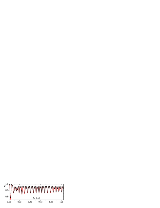
Figure 7: (Color online) Comparison of the polymer chain orientation disorder averaged exact relation Eq. (10) (black points) and approximation Eq. (31) (red line).

Direct numerical evaluation of modulation depths from Eq. (13) shows that, for all orientations of the polymer chains, the maximum modulation depth of the contact hyperfine protons is $0.05$ and the maximum depth of the distant protons is $0.007$ (recall that, for MEH–PPV, in Eqs. (10) and (III) the contact protons are labelled by the subscript, $1\leq j\leq N_{c}$, where $N_{c}=22$, and the distant protons are labelled by $N_{c}<j\leq N$). This allows to approximate the factors in Eqs. (10) and (III) with exponents. For the primary ESEEM one gets:

$$E(2\tau)=\exp\!\left[\!-\!\sum_{j=1}^{N}\!2k_{j}\sin^{2}\!\left(\frac{\omega_{j+}\tau}{2}\right)\!\sin^{2}\!\left(\frac{\omega_{j-}\tau}{2}\right)\!\right]\!.$$ (30)

To some extent, the argument in Eq. (30) is characterized by the sum of all depths, $\kappa=\sum_{j=1}^{N}k_{j}$. With the polymer orientation, $\kappa$ varies between 0.03 and 0.242, and averages at about 0.136. The contribution of distant protons in this sum, $\kappa_{d}=\sum_{j>N_{c}}k_{j}$, is less than 0.06, with the average over the orientation disorder, $\langle\kappa_{d}\rangle=0.047$. Dominant in $\kappa$ is the contribution of contact hyperfine protons, $\kappa_{c}=\sum_{j=1}^{N_{c}}k_{j}$, which has a maximum of 0.2 and averages at about 0.089. However, the contact hyperfine protons have a large dispersion of modulation frequencies, and even relatively large fluctuations of $\kappa_{c}$ do not generate a large argument in Eq. (30). Therefore it is reasonable to expand the exponent (30) and write:

$$E(2\tau)\approx 1-\sum_{j=1}^{N}2k_{j}\sin^{2}\!\left(\frac{\omega_{j+}\tau}{2}\right)\!\sin^{2}\!\left(\frac{\omega_{j-}\tau}{2}\right).$$ (31)

This approximation is further reinforced by averaging Eqs. (10) and (31) over orientation disorder numerically and comparing the results in Fig. 7. After a simple transformation Eq. (31) goes into Eq.(IV.1) of the main text.

The approximation Eq. (15) in the main text for the distant protons is based on the fact that the polaron spin coupling to these protons is weak, $A_{j},B_{j}\ll\omega_{I}$. The following arguments substantiate the same approximation for the contact protons. From Eq. (12) it is seen that the approximation error is $\propto B_{j}^{2}/(\omega_{I}\pm A_{j}/2)$. Consistent with this, we numerically find the largest error, $\omega_{j+}-(\omega_{I}+A_{j}/2)\approx 0.1$ MHz, occurring for the largest $B_{j}$. It results for a C–H proton at vinyl site E, when the external magnetic field is parallel to $\hat{\mathbf{x}}+\hat{\mathbf{y}}$ in the principal axes at E (see Fig. 1). This error is about $1\%$ of the corresponding frequency values, so the approximation is quite accurate.

The stimulated ESEEM is analyzed in a similar way. By virtue of small values of $k_{j}$, Eq. (III) is reduced to the sum Eq. (IV.2) in the main text. After averaging over the disorder in polymer chain orientations and separating the contact and distant proton contributions $\langle E_{\beta}(\tau,T)\rangle$, $\beta=d$, $c$, one gets

$$\langle E_{\beta}(\tau,T)\rangle=-\frac{1}{2}\kappa_{\beta}+\frac{1}{2}F_{\beta}(\tau)\cos\omega_{I}\tau$$

$$\hskip 42.67912pt+\frac{1}{2}F_{\beta}(\tau+T)\cos\omega_{I}[\tau+T]$$ (32)

$$-\frac{1}{4}F_{\beta}(T)\cos\omega_{I}[2\tau+T]-\frac{1}{4}F_{\beta}(2\tau+T)\cos\omega_{I}T,$$

from which Eq. (20) of the main text is written.

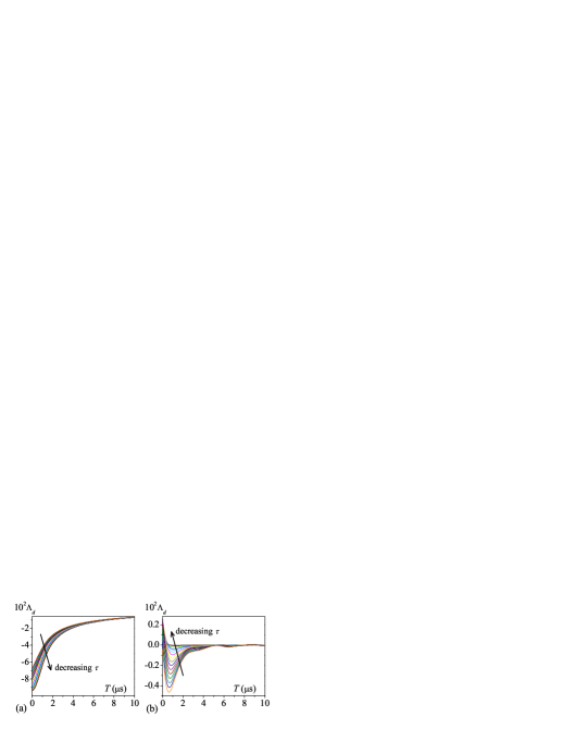
Figure 8: (Color online) Plots of the amplitude, $\Lambda_{d}(\tau_{n},T)$, versus $T$ at fixed $\tau_{n}=(\pi/\omega_{I})n$, for (a) odd $n=1,3,..,29$, and (b) even $n=2,4,..,30$. The plots demonstrate the reduction of $\Lambda_{d}(\tau_{n},T)$ when going from odd to even $n$. For small $n$ the decrease of $\Lambda_{d}(\tau_{n},T)$ from odd to even $n$ is more than two orders of magnitude. For large $n$ it is more that 15 times.

The $T$- dependence of $\langle E_{d}(\tau,T)\rangle$ is simple modulation with the frequency $\omega_{I}$. To find its $\tau$- dependence we rewrite the modulation part of Eq. (A) as

$$\langle E_{\beta}(\tau,T)\rangle\simeq\frac{1}{2}\Lambda_{\beta}(\tau,T)\cos\bigl{(}\omega_{I}T+\varphi_{\beta}(\tau,T)\bigr{)},$$ (33)

with $\varphi_{\beta}=\arg Z_{\beta}(\text{mod }\pi)$ and $\Lambda_{\beta}=Z_{\beta}e^{-i\varphi_{\beta}}$, where

$$Z_{\beta}=e^{i\omega_{I}\tau}F_{\beta}(\tau+T)-\frac{1}{2}e^{2i\omega_{I}\tau}F_{\beta}(T)-\frac{1}{2}F_{\beta}(2\tau+T).$$ (34)

As defined, $\Lambda_{d}(\tau,T)$ and $\varphi_{d}(\tau,T)$ are smooth functions of $T$, varying insignificantly at times, $T\sim 1/\omega_{I}$. In contrast, their $\tau$- dependence is abrupt, because of the presence of exponential factors in Eq. (34). The largest and smallest values of $\Lambda_{d}(\tau,T)$ for a fixed $T$ can be found in an adiabatic accuracy, by differentiating the fast exponents with respect to $\tau$, while regarding the $F_{d}$ factors as constants. It is in fact more convenient to use the relation, $\Lambda_{d}^{2}=|Z_{d}|^{2}$, and differentiate $|Z_{d}|^{2}$. One gets:

$$\partial_{\tau}|Z_{d}|^{2}\approx\omega_{I}\sin\omega_{I}\tau\bigl{[}F_{d}(\tau+T)F_{d}(2\tau+T)$$ (35)

$$\quad+F_{d}(T)F_{d}(\tau+T)-2\cos\omega_{I}\tau F_{d}(T)F_{d}(2\tau+T)\bigr{]}.$$

This yields minima at $\omega_{I}\tau_{n}=\pi n$ for even integer $n$ and maxima at $\omega_{I}\tau_{n}=\pi n$ for odd integer $n$, as expected.

Figure 9: (Color online) The amplitude, $\Lambda_{c}(\tau_{n},T)$, is plotted versus $T$ at fixed $\tau_{n}=(\pi/\omega_{I})n$, for (a) odd $n=1,..,19$, and (b) even $n=2,..,20$. Though the individual curves are not well resolved, it is seen that there is no notable difference in the orders of magnitude of $\Lambda_{c}(\tau_{n},T)$ with even and odd $n$.

To visualize the modulation reduction, in Fig. 8 we plot $\Lambda_{d}(\tau_{n},T)$ against $T$ for $n=1,..,30$. We note that these $\tau_{n}$ include all possible critical values within the interval, $0<\tau<1\,\mu s$, which covers the experimentally available $\tau$- domain, taking into account the decay of the signal in a real experiment. It is seen that for small $n$ the reduction is more than two orders of magnitude, and for large $n$ it is more than 15 times.

For the contribution of contact hyperfine protons, $\langle E_{c}(\tau,T)\rangle$, the modulation given by Eqs. (A) and (33) cannot be interpreted as having a single frequency, because the function $F_{c}$, and therefore $\Lambda_{c}(\tau,T)$ and $\varphi_{c}(\tau,T)$, vary abruptly on the timescale, $T\sim 1/\omega_{I}$. Still, $\Lambda_{c}(\tau,T)$ gives the overall strength of this modulation and it is useful to inspect this quantity for the above critical values of $\tau$. Figure 9 plots $\Lambda_{c}(\tau_{n},T)$ versus $T$ for the first 20 values of $\tau_{n}$. Overall, the magnitudes of $\Lambda_{c}(\tau_{n},T)$ in Fig. 9 are close to each other for even and odd $n$, meaning that there is no reduction of the corresponding modulation. From Fig. 9 we also infer that $\Lambda_{c}(\tau_{n},T)$, and therefore $\langle E_{c}(\tau_{n},T)\rangle$, is very small for $T>0.5\,\mu$s, and nearly vanishes for $T>0.75\,\mu$s.

Appendix B

In this Appendix we outline the generalization of Eqs (10), (III) for an ensemble of polarons hopping over the polymer sites of random orientations. Consider pulse sequences similar to those in Fig. 2(a), but with unequal delay times; $\pi/2$ - $\tau_{1}$ - $\pi$ - $\tau_{2}$ - $echo$, and $\pi/2$ - $\tau_{1}$ - $\pi/2$ - $T$ - $\pi/2$ - $\tau_{2}$ - $echo$. Using the density matrix formalism, the modulation functions are

$$E(\tau_{1},\tau_{2})=\mathcal{N}\,\text{Tr}\left[U(\tau_{1},\tau_{2})\hat{\rho}(0)U^{\dagger}(\tau_{1},\tau_{2})S^{y}\right],$$ (36)

$$E(\tau_{1},T,\tau_{2})=\mathcal{N}\,\text{Tr}\left[U(\tau_{1},T,\tau_{2})\hat{\rho}(0)U^{\dagger}(\tau_{1},T,\tau_{2})S^{y}\right],$$

where $\hat{\rho}(0)\propto(1/2+S^{z})$ is the initial density operator introduced in Eq. (8) and $\mathcal{N}^{-1}=\text{Tr}\bigl{(}[3\pi/2]\hat{\rho}(0)[3\pi/2]^{\dagger}S^{y}\bigr{)}$ is the normalization factor. The evolution operators are given by

$$U(\tau_{1},\tau_{2})=e^{-i\tau_{2}\tilde{H}}\bigl{[}\pi\bigr{]}e^{-i\tau_{1}\tilde{H}}\bigl{[}\pi/2\bigr{]},$$ (37)

$$U(\tau_{1},T,\tau_{2})=e^{-i\tau_{2}\tilde{H}}\bigl{[}\pi/2\bigr{]}e^{-iT\tilde{H}}\bigl{[}\pi/2\bigr{]}e^{-i\tau_{1}\tilde{H}}\bigl{[}\pi/2\bigr{]},$$

where $\tilde{H}$ is Hamiltonian (1) in the coordinate system rotating around $\hat{\mathbf{z}}$ with the frequency $\Omega$. For later reference, we also consider the free induction decay,

$$F(t)=-\mathcal{N}\,\text{Tr}\left[e^{-it\tilde{H}}\bigl{[}\pi/2\bigr{]}\hat{\rho}(0)\bigl{[}\pi/2\bigr{]}^{\dagger}e^{it\tilde{H}}S^{y}\right].$$ (38)

By taking the traces over the polaron spin space, Eqs. (36), (38) are reduced to the nuclear spin traces, involving the nuclear spin Hamiltonians,

$$h^{\pm}=\pm\frac{1}{2}\sum_{j=1}^{N}\bigl{(}A_{j}I^{z}_{j}+B_{j}I^{x}_{j}\bigr{)}-\sum_{j=1}^{N}\omega_{I}I^{z}_{j}.$$ (39)

Subsequently, the nuclear spin traces are calculated explicitly. More specifically, we have:

$$F(t)=2^{-N}\text{Tr}_{I}\!\left[e^{-ith^{-}}e^{ith^{+}}\right]=\prod_{j=1}^{N}f_{j}(t),$$ (40)

$$E(\tau_{1},\tau_{2})=2^{-N}\text{Tr}_{I}\!\left[e^{-i\tau_{2}h^{+}}e^{-i\tau_{1}h^{-}}e^{i\tau_{1}h^{+}}e^{i\tau_{2}h^{-}}\right]=\prod_{j=1}^{N}\epsilon_{j}(\tau_{1},\tau_{2}),$$ (41)

$$E(\tau_{1},T,\tau_{2})=2^{-N-1}\text{Tr}_{I}\!\left[e^{-i(\tau_{2}+T)h^{+}}e^{-i\tau_{1}h^{-}}e^{i(\tau_{1}+T)h^{+}}e^{i\tau_{2}h^{-}}\right]\!+\bigl{(}\!+\leftrightarrow-\!\bigr{)}^{\ast}=\frac{1}{2}\!\prod_{j=1}^{N}\!\epsilon_{j}^{+}(\tau_{1},T,\tau_{2})+\bigl{(}\!+\leftrightarrow-\!\bigr{)}^{\ast},\quad$$ (42)

where $(\!+\leftrightarrow-\!)^{\ast}$ denote the complex conjugates of previous expressions with the superscripts swapped, and the functions

$$f_{j}(t)=\cos\frac{\omega_{j+}t}{2}\cos\frac{\omega_{j-}t}{2}+\frac{\omega_{I}^{2}-A_{j}^{2}/4-B_{j}^{2}/4}{\omega_{j+}\omega_{j-}}\sin\frac{\omega_{j+}t}{2}\sin\frac{\omega_{j-}t}{2},$$ (43)

$$\epsilon_{j}(t_{1},t_{2})=f_{j}(t_{1}-t_{2})-2k_{j}\sin\frac{\omega_{j+}t_{1}}{2}\sin\frac{\omega_{j-}t_{1}}{2}\sin\frac{\omega_{j+}t_{2}}{2}\sin\frac{\omega_{j-}t_{2}}{2},$$

$$\epsilon_{j}^{\pm}(t_{1},T,t_{2})=f_{j}(t_{1}-t_{2})-2k_{j}\sin\frac{\omega_{j\pm}(t_{1}+T)}{2}\sin\frac{\omega_{j\pm}(t_{2}+T)}{2}\sin\frac{\omega_{j\mp}t_{1}}{2}\sin\frac{\omega_{j\mp}t_{2}}{2},$$

are introduced, with $\omega_{j\pm}$ and $k_{j}$ given in Eqs. (12), (13).

Figure 10: (Color online) Schematic definitions of polaron random walk trajectories, $\mathbf{R}(t)$, for free induction decay (a), and primary echo (b). The blue lines denote the pulses. The green lines show the detection points. The red bars are polaron random hops.

To generalize Eqs. (40) for hopping polarons, consider a polaron random walk right after the initial $\pi/2$-pulse (time $t=0$) from some polymer site, $\mathbf{r}_{0}$. Its trajectory, $\mathbf{R}(t)$, specifies the waiting time, $\delta t_{n}$, which the polaron spends at $\mathbf{r}_{n}$. Other necessary details of $\mathbf{R}(t)$ are represented in Fig. 10(a), showing that for time $t$ the polaron performes $M$ hops, arriving in the site $\mathbf{r}_{M}$ time $\delta t^{\prime}_{M}$ before the detection. The prime indicates that $\delta t^{\prime}_{M}$ is not the total waiting time at $\mathbf{r}_{M}$. By this definition,

$$t=\delta t^{\prime}_{M}+\sum_{n=0}^{M-1}\delta t_{n},\qquad\delta t_{M}=\delta t^{\prime}_{M}+\delta t^{\prime\prime}_{M},$$ (44)

The free induction decay of a polaron undergoing such a random walk is given by

$$F_{\mathbf{R}}(t)=2^{1-N(M+1)}\,\text{Tr}\left[u_{\mathbf{R}}(t)S^{y}u_{\mathbf{R}}^{\dagger}(t)S^{y}\right],$$ (45)

with the time-ordered operator $u_{\mathbf{R}}(t)$, replacing the exponential factors in Eq. (38),

$$u_{\mathbf{R}}(t)=e^{-i\delta t^{\prime}_{M}H_{M}}\prod\limits_{n=0}^{{M-1}\atop\longleftarrow}e^{-i\delta t_{n}H_{n}}.$$ (46)

Here the arrow indicates the inverse order of factors in the products. The transient Hamiltonians in Eq. (46) are

$$H_{n}=\sum_{j=1}^{N}S^{z}\bigl{(}A_{j,\mathbf{r}_{n}}I^{z}_{j,\mathbf{r}_{n}}+B_{j,\mathbf{r}_{n}}I^{x}_{j,\mathbf{r}_{n}}\bigr{)}-\sum_{l=0}^{M}\sum_{j=1}^{N}\omega_{I}I^{z}_{j,\mathbf{r}_{l}},$$ (47)

where $\mathbf{I}_{j,\mathbf{r}}$ is the spin operator and $A_{j,\mathbf{r}}$, $B_{j,\mathbf{r}}$ are the hyperfine coupling constants of the $j$-th proton located at site $\mathbf{r}$, and the sum over $l$ includes all $M+1$ molecular sites visited for the random walk $\mathbf{R}(t)$. The time dependence of the spin Hamiltonian is thus incorporated in the second term of Eq. (47), describing the hyperfine coupling of the polaron spin with protons near the site, $\mathbf{r}_{n}=\mathbf{R}(t)$, occupied by the polaron at time $t$.

The trace over the polaron spin space in Eq. (45) can be easily taken as the transient Hamiltonians (47) conserve $S^{z}$. The result is written in terms of the trace over the nuclear spins:

$$F_{\mathbf{R}}(t)=2^{-N(M+1)}\text{Tr}_{I}\!\left[u_{\mathbf{R},-}(t)u_{\mathbf{R},+}^{\dagger}(t)\right].$$ (48)

where we have introduced

$$u_{\mathbf{R},\pm}(t)=e^{-i\delta t^{\prime}_{M}h_{M}^{\pm}}\!\!\prod\limits_{n=0}^{{M-1}\atop\longleftarrow}e^{-i\delta t_{n}h_{n}^{\pm}}.$$ (49)

The spin Hamiltonians, $h_{n}^{\pm}$, are given by Eq. (39), with the coupling constants and spin operators of protons at $\mathbf{r}_{n}$. Note that unlike Eq. (47), the last term in Eq. (39) involves nuclear spin operators only for a single site. This simplification is general for transport models neglecting the polaron returns to the sites visited previously, such as the multiple trapping model adopted in this study. Moreover, neglecting the polaron returns allows to calculate the trace in Eq. (48) explicitly. One finds:

$$F_{\mathbf{R}}(t)=\left(\prod\limits_{n=0}^{M-1}F_{n}(\delta t_{n})\right)F_{M}(\delta t^{\prime}_{M}),$$ (50)

where $F_{n}(t)$ is the free induction decay Eq. (40) calculated for the single site, $\mathbf{r}_{n}$.

Similar expressions can be written for the primary and stimulated ESE modulation functions, provided the polaron random walk trajectory is specified relative to the pulse sequence. Namely, for the primary sequence let $\mathbf{R}(\tau_{1}+\tau_{2})=\mathbf{r}_{M}$, and the instantaneous $\pi$-pulse is applied $\delta t^{\prime}_{M_{1}}$ time after the polaron arrives in the site $\mathbf{r}_{M_{1}}$, and $\delta t^{\prime\prime}_{M_{1}}$ time before it makes the next hop, see Fig. 10(b). The primary ESE modulation from a spin with this trajectory is found to be

$$E_{\mathbf{R}}(\tau_{1},\tau_{2})=\left(\prod\limits_{n=0}^{M_{1}-1}F_{n}(\delta t_{n})\right)\!E_{M_{1}}(\delta t^{\prime}_{M_{1}},\delta t^{\prime\prime}_{M_{1}})\quad$$ (51)

$$\times\left(\prod\limits_{n=M_{1}+1}^{M-1}F_{n}(\delta t_{n})\right)\!F_{M}(\delta t^{\prime}_{M}),$$

where $E_{n}(t_{1},t_{2})$ is the modulation function (41), for $\mathbf{r}_{n}$.

The stimulated ESE modulation critically depends on whether a random walk involves a hop in the interval $T$ or not. We separate these cases in Fig. 11(a) and (b). The trajectories with no hops during the interval $T$, Fig. 11(a), are denoted by $\mathbf{R}_{0}$, while those incorporating hops in $T$, Fig. 11(b), by $\mathbf{R}_{1}$. With the further details of trajectories specified in Fig. 11, one gets:

$$E_{\mathbf{R}_{0}}(\tau_{1},T,\tau_{2})\!\!\!\! =\left(\prod\limits_{n=0}^{M_{1}-1}F_{n}(\delta t_{n})\right)\!E_{M_{1}}(\delta t^{\prime}_{M_{1}},T,\delta t^{\prime\prime}_{M_{1}})$$ (52)

$$\times\left(\prod\limits_{n=M_{1}+1}^{M-1}F_{n}(\delta t_{n})\right)\!F_{M}(\delta t^{\prime}_{M}),$$

where $E_{n}(t_{1},T,t_{2})$ is is given by Eq. (42) at $\mathbf{r}_{n}$, and

$$E_{\mathbf{R}_{1}}(\tau_{1},T,\tau_{2})=\left(\prod\limits_{n=0}^{M_{1}-1}F_{n}(\delta t_{n})\right)F_{M_{1}}(\delta t^{\prime}_{M_{1}})$$

$$\times F_{M_{2}}(\delta t^{\prime\prime}_{M_{2}})\left(\prod\limits_{n=M_{2}+1}^{M-1}F_{n}(\delta t_{n})\right)\!F_{M}(\delta t^{\prime}_{M}).$$ (53)

Figure 11: (Color online) Illustration of notations for polaron random walk trajectories during the stimulated pulse sequence. The blue bars symbolize the pulses. The green bars show the detection. The red lines are polaron random hops. (a) Trajectories of type $\mathbf{R}_{0}$, Eq. (52); no polaron hop occurs in the time interval $T$. (b) Trajectories of type $\mathbf{R}_{1}$, Eq. (52); at least one hop occurs in the time interval $T$.

Finally, the free induction decay and ESE modulations of the ensemble of randomly walking polarons is found from Eqs. (50) – (B), via averaging over the random-walk trajectories:

$$\mathcal{F}(t)=\left\langle F_{\mathbf{R}}(t)\right\rangle_{\{\mathbf{R}\}},$$ (54)

$$\mathcal{E}(\tau_{1},\tau_{2})=\left\langle E_{\mathbf{R}}(\tau_{1},\tau_{2})\right\rangle_{\{\mathbf{R}\}},$$ (55)

$$\mathcal{E}(\tau_{1},T,\tau_{2})=\left\langle E_{\mathbf{R}}(\tau_{1},T,\tau_{2})\right\rangle_{\{\mathbf{R}\}}.$$ (56)

The averages are evaluated numerically, by a Monte Carlo sampling of random walk trajectories, including the random on-site trapping energies defining the waiting time statistics via Eq. (21). In our simulations we also incorporate the random orientations of polymer chains.

Appendix C

In this Appendix we investigate $\mathcal{F}(t)$, $\mathcal{E}(\tau,T)$, and $\mathcal{E}(\tau_{1},T,\tau_{2})$ analytically, within the multiple trapping model at $\alpha\to\infty$. This implies uniform hopping rates, $W_{\mathbf{r}}=\nu$, entailing the Poissonian waiting time distribution, $P(\delta t)=\nu\exp(-\nu\delta t)$. In this limit the free induction decay satisfies a Dyson-type integral equation, Kubo79 ; Allodi14

$$\mathcal{F}(t)=g(t)e^{-\nu t}+\nu\int_{0}^{t}\!\!dt^{\prime}e^{-\nu t^{\prime}}g(t^{\prime})\mathcal{F}(t-t^{\prime}),$$ (57)

where the on-site relaxation function,

$$g(t)=\bigl{\langle}F(t)\bigr{\rangle},$$ (58)

is introduced. Here, $F(t)$ is given by Eq. (40), and the brackets mean the average over random orientations of molecular sites. In Eq. (57) the first term is the relaxation if for time $t$ the polarons do not hop, which occurs with the probability $e^{-\nu t}$, and the integral accounts for the relaxation with the first hop happening at time $t^{\prime}<t$.

The formal solution of Eq. (57) is given in terms of the Laplace transform:

$$\tilde{\mathcal{F}}(s)=\frac{\tilde{g}(s+\nu)}{1-\nu\tilde{g}(s+\nu)},$$ (59)

where $\tilde{f}(s)=\int_{0}^{\infty}\exp(-st)f(t)dt$ denotes the Laplace transform of $f(t)$. However, from this equation $\mathcal{F}(t)$ can be found only numerically, as the inverse Laplace transform of Eq. (59) is not accessible analytically.

Semiclassical description

A semiclassical approximation for $\mathcal{F}$ and $\mathcal{E}$ follows upon replacing the Hamiltonian in Eqs. (37), (38) by its semiclassical counterpart, Eq. (7). The resulting on-site free induction decay has the simple form,

$$g_{0}(t)=\langle\cos(\omega_{z}t)\rangle_{\omega_{z}}=\exp\bigl{(}-\omega_{\text{hf}}^{2}t^{2}/2\bigr{)}.$$ (60)

Still, the solution for the semiclassical free induction decay, $\mathcal{F}_{0}(t)$, using the inverse Laplace transform (59), can be found only numerically. Allodi14

In what follows we give a perturbative treatment for the semiclassical echo modulation functions, $\mathcal{E}_{\text{SC}}(2\tau)=\mathcal{E}(\tau,\tau)$ and $\mathcal{E}_{\text{SC}}(\tau,T)=\mathcal{E}(\tau,T,\tau)$, from which Eqs. (22) and (26) of the main text result. In the semiclassical approximation and within the multiple trapping model at $\alpha\to\infty$, Eqs. (54) – (56) can be relates as

$$\mathcal{E}_{\text{SC}}(2\tau)=e^{-2\nu\tau}\left[1+2\nu\int_{0}^{\tau}e^{2\nu t}\mathcal{F}_{0}^{\,2}(t)dt\right],$$ (61)

$$\mathcal{E}_{\text{SC}}(\tau,T)=e^{-\nu T}\mathcal{E}_{\text{SC}}(2\tau)+\mathcal{F}_{0}^{\,2}(\tau)\left(1-e^{-\nu T}\right),\quad\qquad$$ (62)

detailed derivation of which will be given elsewhere. MDunp Thus, $\mathcal{E}_{\text{SC}}(2\tau)$ and $\mathcal{E}_{\text{SC}}(\tau,T)$ are determined by $\mathcal{F}_{0}(t)$. Note that the first term in Eq. (62) is the contribution of type $\mathbf{R}_{0}$ trajectories, Fig. 11(a), while the last term is that of the type $\mathbf{R}_{1}$ trajectories, Fig. 11(b).

In the regime of slow hopping, $\eta\equiv\nu/\omega_{\text{hf}}\ll 1$, a reasonably good approximation can be made for $\mathcal{F}_{0}(t)$ from Eq. (57) iteratively. To the linear order in $\eta$ one gets:

$$\mathcal{F}_{0}(t)=e^{-\nu t}\left[g_{0}(t)+\nu\int_{0}^{t}\!\!dt^{\prime}g_{0}(t^{\prime})g_{0}(t-t^{\prime})\right].$$ (63)

Using this in Eq. (61) leads to Eq. (22) in the main text. Equation (63) also shows that the decay of $\mathcal{F}_{0}(t)$ is nearly Gaussian and fast, so that for $\tau>1/\omega_{\text{hf}}$ the last term in Eq. (62) can be neglected, and Eq. (26) in the main text can be written.

In the fast hopping regime, $\eta\gg 1$, the Laplace transform appears to be useful. One has:

$$\mathcal{F}_{0}(t)=\frac{1}{2\pi i}\int_{-i\infty}^{i\infty}\!\!\!ds\,e^{st}\tilde{\mathcal{F}}_{0}(s),$$ (64)

with $\tilde{\mathcal{F}}_{0}(s)$ given by Eq. (59) and the Laplace transform,

$$\tilde{g}_{0}(s)=\sqrt{\pi/2}\,\omega_{\text{hf}}^{-1}\exp\bigl{(}s^{2}/2\omega_{\text{hf}}^{2}\bigr{)}\text{erfc}\bigl{(}s/\sqrt{2}\omega_{\text{hf}}\bigr{)},$$ (65)

where $\text{erfc}(x)$ is the complementary error function. $\tilde{\mathcal{F}}_{0}(s)$ is holomorphic on the complex half-plane, $\text{Re}(s)<0$, excluding the simple poles determined by the denominator of Eq. (59). A thorough analysis of the inverse Laplace transform (64) shows that $\tilde{\mathcal{F}}_{0}(s)$ has one real negative pole, $s_{0}$, and infinitely many complex poles. MDunp Also, for $\eta\gg 1$ the contribution of $s_{0}$ dominates in the integral (64), giving $\mathcal{F}_{0}(t)=-(\omega_{\text{hf}}^{2}/\nu s_{0})\exp(s_{0}t)$. From the large-argument asymptote of Eq. (65) one finds $s_{0}=-\omega_{\text{hf}}^{2}/\nu$, leading to the well-known result in the motional narrowing regime, $\mathcal{F}_{0}(t)=\exp(-\omega_{\text{hf}}^{2}\,t/\nu)$. With this $\mathcal{F}_{0}(t)$, the integral term in Eq. (61) is dominant, yielding $\mathcal{E}_{\text{SC}}(2\tau)=\exp(-2\,\omega_{\text{hf}}^{2}\,\tau/\nu)$.

References

- (1) S. R. Forrest, Nature (London) 428, 911 (2004).
- (2) Special issue on organic electronics and optoelectronics. Chem. Rev. 107, 923 (2007).
- (3) J. Shinar, Laser Photonics Rev. 6, 767 (2012).
- (4) B. C. Cavenett, Adv. Phys. 30, 475 (1981).
- (5) R. A. Street, Phys. Rev. B 26, 3588 (1982).
- (6) S. Depinna, B. C. Cavenett, I. G. Austin, T. M. Searle, M. J. Thompson, J. Allison, and P. G. L. Comberd, Philos. Mag. B 46, 473 (1982).
- (7) M. Stutzmann, M. S. Brandt, and M. W. Bayerl, J. Non-Cryst. Solids 266 269, 22 (2000).
- (8) E. Lifshitz, L. Fradkin, A. Glozman, and L. Langof, Annu. Rev. Phys. Chem. 55, 509 (2004).
- (9) D. R. McCamey, H. Huebl, M. S. Brandt, W. D. Hutchison, J. C. McCallum, R. G. Clark, and A. R. Hamilton, Appl. Phys. Lett. 89, 182115 (2006).
- (10) D. R. McCamey, H. A. Seipel, S.-Y. Paik, M. J. Walter, N. J. Borys, J. M. Lupton, and C. Boehme, Nat. Mater. 7, 723 (2008).
- (11) D. R. McCamey, K. J. van Schooten, W. J. Baker, S.-Y. Lee, S.-Y. Paik, J. M. Lupton, and C. Boehme, Phys. Rev. Lett. 104, 017601 (2010).
- (12) D. R. McCamey, S.-Y. Lee, S.-Y. Paik, J. M. Lupton, and C. Boehme, Phys. Rev. B 82, 125206 (2010).
- (13) J. Behrends, A. Schnegg, K. Lips, E. A. Thomsen, A. K. Pandey, I. D. W. Samuel, and D. J. Keeble, Phys. Rev. Lett. 105, 176601 (2010).
- (14) W. J. Baker, T. L. Keevers, J. M. Lupton, D. R. McCamey, and C. Boehme, Phys. Rev. Lett. 108, 267601 (2012).
- (15) H. Malissa, M. Kavand, D. P. Waters, K. J. van Schooten, P. L. Burn, Z. V. Vardeny, B. Saam, J. M. Lupton, and C. Boehme, Science 345, 1487 (2014).
- (16) K. J. van Schooten, D. L. Baird, M. E. Limes, J. M. Lupton, and C. Boehme, Nat. Commun. 6, 6688 (2015).
- (17) C. P. Slichter, Principles of Magnetic Resonance (Harper & Row, New York, 1963).
- (18) V. A. Dediu, L. E. Hueso, I. Bergenti, and C. Taliani, Nat. Mater. 8, 850 (2009).
- (19) T. Nguyen, G. Hukic-Markosian, F. Wang, L. Wojcik, X. Li, E. Ehrenfreund, Z. Vardeny, Nat. Mater. 9, 345 (2010).
- (20) S. A. Dikanov and Y. D. Tsvetkov, Electron Spin Echo Envelope Modulation (ESEEM) spectroscopy (CRC Press, Boca Raton, FL, 1992).
- (21) A. Schweiger and G. Jeschke, Principles of Pulsed Electron Paramagnetic Resonance (Oxford University Press, Oxford, UK, 2001).
- (22) K. Schulten and P. G. Wolynes, J. Chem. Phys. 68, 3292 (1978).
- (23) A. Abragam, Principles of Nuclear Magnetism (Oxford University Press, New York, 1961).
- (24) S. Kuroda, T. Noguchi, and T. Ohnishi, Phys. Rev. Lett. 72, 286 (1994).
- (25) S. Kuroda, K. Murata, T. Noguchi, and T. Ohnishi, J. Phys. Soc. Jpn. 64, 1363 (1995).
- (26) S. Kuroda, K. Marumoto, H. Ito, N. C. Greenham, R. H. Friend, Y. Shimoi, and S. Abe, Chem. Phys. Lett. 325, 183 (2000).
- (27) Y. Shimoi, S. Abe, S. Kuroda, and K. Murata, Solid State Commun. 95, 137 (1995).
- (28) S. Kuroda, Appl. Magn. Reson. 23, 455 (2003).
- (29) J. R. Morton, Chem. Rev. 64, 453 (1964).
- (30) L. Claes, J. P. Francois, and M. S. Deleuze, Chem. Phys. Lett. 339, 216 (2001).
- (31) S. Kilina, N. Dandu, E. R. Batista, A. Saxena, R. L. Martin, D. L. Smith, and S. Tretiak, J. Phys. Chem. Lett. 4, 1453 (2013).
- (32) T. Qin and A. Troisi, J. Am. Chem. Soc. 135, 11247 (2013).
- (33) A. Bondi, J. Phys. Chem. 68, 441 (1964).
- (34) I. Motoc and G. R. Marshall, Chem. Phys. Lett. 116, 415 (1985).
- (35) W. J. Spillane, G. G. Birch, M. G. B. Drew, and I. Bartolo, J. Chem. Soc., Perkin Trans. 2, 497 (1992).
- (36) Throughout the paper, by the Fourier transform of a function of two variables, , we mean the transformation over the variable , whereas is kept as a parameter. For the precise definition of these Fourier transforms see Appendix A.
- (37) The largest value of within the HFI under consideration is about MHz, whereas the X – band proton Larmor frequency is about MHz.
- (38) V. V. Mkhitaryan and V. V. Dobrovitski, Phys. Rev. B 92, 054204 (2015).
- (39) R. C. Roundy and M. E. Raikh, Phys. Rev. B 90, 201203 (2014).
- (40) R. Czech and K. W. Kehr, Phys. Rev. Lett. 53, 1783 (1984); Phys. Rev. B 34, 261 (1986).
- (41) P. Mitra and P. Le Doussal Phys. Rev. B 44, 12035 (1991).
- (42) R. S. Hayano, Y. J. Uemura, J. Imazato, N. Nishida, T. Yamazaki, and R. Kubo, Phys. Rev. B 20, 850 (1979).
- (43) A. Jakobs and K. W. Kehr, Phys. Rev. B 48, 8780 (1993).
- (44) B. Hartenstein, H. Bassler, A. Jakobs, and K. W. Kehr, Phys. Rev. B 54, 8574 (1996).
- (45) N. J. Harmon and M. E. Flatté, Phys. Rev. Lett. 110, 176602 (2013).
- (46) N. J. Harmon and M. E. Flatté, Phys. Rev. B 90, 115203 (2014).
- (47) V. Coropceanu, J. Cornil, D. A. da Silva Filho, Y. Olivier, R. Silbey, and J.-L. L. Brèdas, Chem. Rev. 107, 926 (2007).
- (48) P. W. M. Blom and M. C. J. M. Vissenberg, Mater. Sci. Eng., R 27, 53 (2000).
- (49) Z. Yue, V. V. Mkhitaryan, and M. E. Raikh, arXiv: 1602.00785.
- (50) D. Kaplan, I. Solomon, and N. F. Mott, J. Phys. (Paris) 39, L51 (1978).
- (51) G. Zwanenburg and P. J. Hore, J. Magn. Reson. A 114, 139 (1995).
- (52) G. Allodi and R. De Renzi, Phys. Scr. 89, 115201 (2014).
- (53) V. V. Mkhitaryan and V. V. Dobrovitski, unpublished.